1 Introduction
Benjamin’s (Reference Benjamin1968) analysis of the steady-state gravity current (GC) is a fundamental and seminal theoretical contribution to the field. The considered configuration was: a layer of fluid of density
 $\unicode[STIX]{x1D70C}_{1}$
and height
 $h$
(the ‘current’) propagating with constant speed
 $U$
into another motionless fluid of density
 $\unicode[STIX]{x1D70C}_{2}~({<}\unicode[STIX]{x1D70C}_{1})$
and height
 $H~({>}h)$
(the ‘ambient’). Shear effects on the boundaries of the system are neglected. This renders a reduction to a large domain of flows, with essentially an infinite number of combinations of densities
 $\unicode[STIX]{x1D70C}_{1},\unicode[STIX]{x1D70C}_{2}$
and heights
 $h,H$
, into one compact result: the ratio
 $Fr=U/(g^{\prime }h)^{1/2}$
is a function of
 $a=h/H$
only (here
 $g^{\prime }$
is the reduced gravity; see (2.1)). The solution of Benjamin provides an analytical expression
 $Fr(a)$
, and shows that a flow with valid non-negative dissipation exists only for
 $a\leqslant a_{max}=1/2$
. Admittedly, a careful consideration of this derivation gives rise to various objections concerning the applicability to real GCs with large Reynolds number
 $Re=Uh/\unicode[STIX]{x1D708}$
produced by realistic initial conditions and confined by realistic solid boundaries (
 $\unicode[STIX]{x1D708}$
is the typical kinematic viscosity of the fluids). Nevertheless, this is a classical and indispensable prototype result, which still inspires extensions and interpretations (e.g. Klemp, Rotunno & Skamarock Reference Klemp, Rotunno and Skamarock1994, Ungarish Reference Ungarish2006, Reference Ungarish2009, White & Helfrich Reference White and Helfrich2008, Borden & Meiburg Reference Borden and Meiburg2013, Milewski & Tabak Reference Milewski and Tabak2015).
Benjamin’s (Reference Benjamin1968) analysis has been formulated for a very constrained geometry: (i) the cross-section of the channel is rectangular or laterally unbounded; and (ii) the channel has a fixed top at height
 $H$
. In a wide range of practical circumstances the GCs of interest do not fulfil these restrictions: the channel has a non-rectangular confining geometry (e.g. triangle, semi-circle, trapezoid), and the upper surface is open to the atmosphere. The analysis of these cases requires non-trivial extensions of Benjamin’s solution.
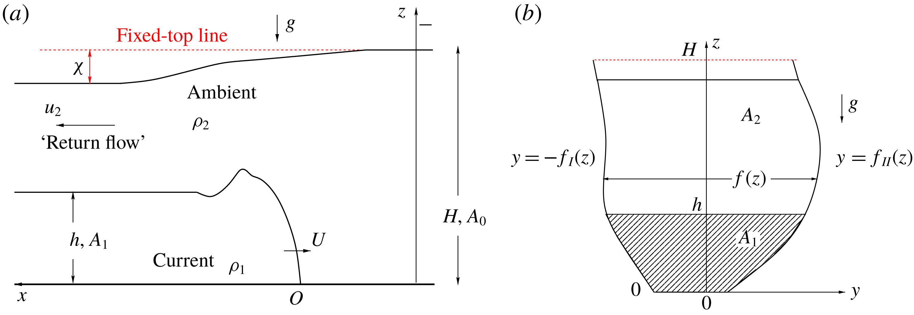
The configuration of interest is sketched in figure 1. The GC flows in the horizontal
 $-x$
direction, the gravity acts in the
 $-z$
direction and the lateral boundaries of the channel are
 $y=-f_{I}(z)$
and
 $y=f_{II}(z)$
. The width function is
 $f(z)=f_{I}(z)+f_{II}(z)$
. We allow for a fairly general cross-section function, but exclude profiles with sharp variation and narrow gaps (
 $f(h)<h$
) where viscous effects may be important. Typical examples are a
 $\vee$
triangle with an apex angle of
 $10^{\circ }$
, say, or larger; a semi-circle; and a trapezoid whose small base is larger than
 $h$
. The value of
 $h$
is sufficiently large for justifying the large
 $Re$
assumption.
It is convenient to introduce the cross-section areas of the unperturbed upstream ambient, and of the downstream current and ambient, as
 $$\begin{eqnarray}A_{0}=\int _{0}^{H}f(z)\,\text{d}z;\quad A_{1}=\int _{0}^{h}f(z)\,\text{d}z;\quad A_{2}=\int _{h}^{H-\unicode[STIX]{x1D712}}f(z)\,\text{d}z.\end{eqnarray}$$
Schematic description of the idealized GC system in the laboratory frame. (a) The
 $xz$
plane view and (b) cross-section
 $yz$
view. The free-top surface is open to constant pressure
 $p=0$
.

Plots of
 $Fr_{f}$
for fixed-top system as a function of
 $a=h/H$
for the various cross-sections considered here, in the range of validity (rate of dissipation
 $\dot{{\mathcal{D}}}\geqslant 0$
). The
 $f(z)$
shapes are also sketched: power-law
 $z^{\unicode[STIX]{x1D6FC}}$
with
 $\unicode[STIX]{x1D6FC}=0,1/2,1$
(rectangle, semi-circle, triangle); and trapezoid
 $H-\unicode[STIX]{x1D6FD}z$
with
 $\unicode[STIX]{x1D6FD}=0.5$
.

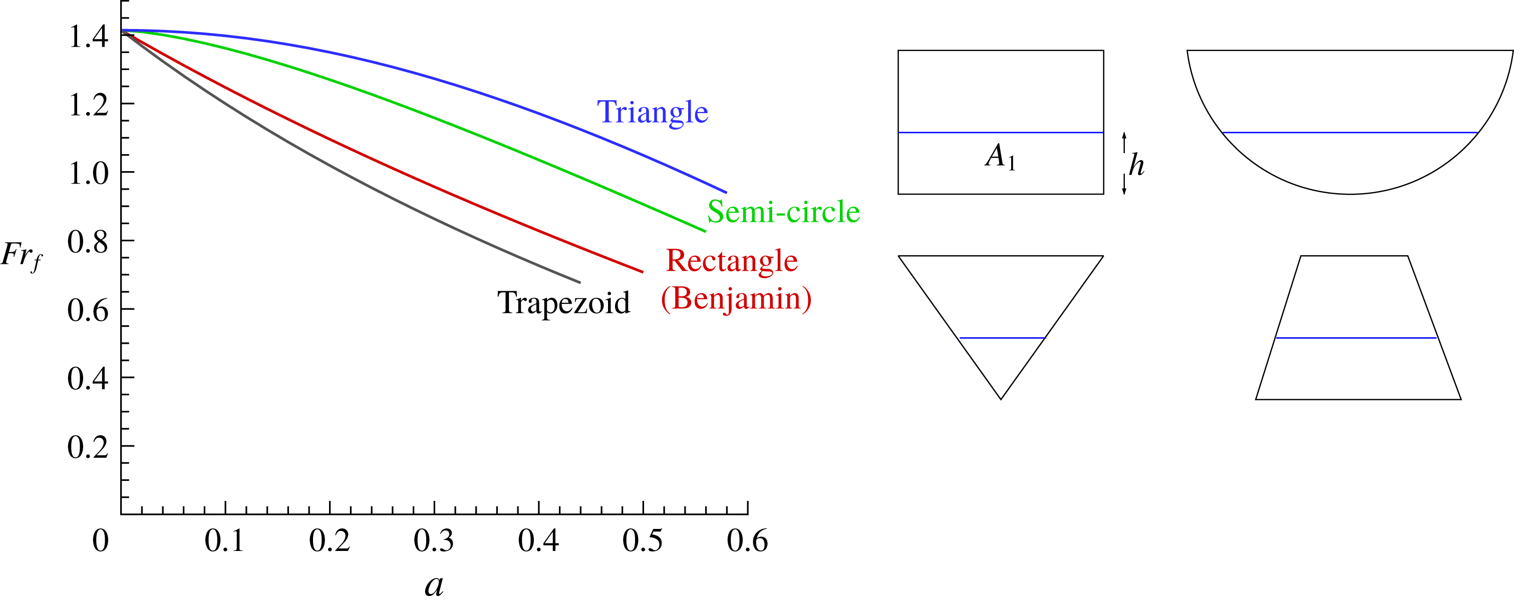
The extension of the analysis to non-rectangular cross-section (but still in the presence of a fixed-top restriction) has been presented by Ungarish (Reference Ungarish2012). The result is that the speed of propagation can be, again, expressed as
 $U=Fr_{f}(a)(g^{\prime }h)^{1/2}$
where
 $$\begin{eqnarray}Fr_{f}^{2}=2\frac{1-\unicode[STIX]{x1D711}}{1+\unicode[STIX]{x1D711}}\left[1-\unicode[STIX]{x1D711}+\frac{1}{\displaystyle hA_{0}}\int _{0}^{h}zf(z)\,\text{d}z\right],\end{eqnarray}$$
and
 $\unicode[STIX]{x1D711}=A_{1}/A_{0}$
is a function of
 $a$
. The subscript
 $f$
denotes the fixed-top case. The energy-validity (non-negative dissipation) restriction is
 $[Fr_{f}/(1-\unicode[STIX]{x1D711})]^{2}\leqslant 2$
which reduces to
 $a\leqslant a_{max}$
depending on
 $f(z)$
. We note that the solution (for a given
 $f(z)$
) depends only on the geometric parameter
 $a=h/H$
, for any density ratio
 $r=\unicode[STIX]{x1D70C}_{2}/\unicode[STIX]{x1D70C}_{1}$
. The classical two-dimensional (2D) case is recovered by
 $f(z)=$
const. Typical results are shown in figure 2. We observe that the cross-section geometry is an important factor in the prediction of the propagation of the GC.
A more formidable restriction of Benjamin’s (Reference Benjamin1968) analysis is the presence of a fixed-height top,
 $z=H$
. Benjamin was aware of the applicability of the steady-state model to other fixed-top cross-sections, and actually presented a special energy-conserving solution for a circle. On the other hand, that paper emphasizes that an insightful simple model is possible ‘if, first, the fluid is given a fixed upper boundary at a finite height above the bottom’ (p. 213). The relaxation of this constraint is more complicated than the previous extension to a non-rectangular channel, because the open-top flow solution involves two unknowns: the speed of propagation and the depression on the surface, i.e.
 $U$
and
 $\unicode[STIX]{x1D712}$
(in scaled form,
 $Fr$
and
 $\tilde{\unicode[STIX]{x1D712}}=\unicode[STIX]{x1D712}/H$
). Moreover, the results are bound to depend on both
 $a$
and
 $r=\unicode[STIX]{x1D70C}_{2}/\unicode[STIX]{x1D70C}_{1}$
. This can be inferred from the following qualitative consideration. In the fixed-top case,
 $\unicode[STIX]{x1D70C}_{2}U^{2}\sim \unicode[STIX]{x0394}\unicode[STIX]{x1D70C}gh$
, where
 $\unicode[STIX]{x0394}\unicode[STIX]{x1D70C}=\unicode[STIX]{x1D70C}_{1}-\unicode[STIX]{x1D70C}_{2}$
. An observer attached to the current notes that the speed of the stream increases significantly from
 $U$
to
 $u_{2}=U/(1-A_{1}/A_{0})$
from front to back, with a corresponding increase of kinetic energy. By opening the top streamline to a constant pressure, that increase of kinetic energy must be balanced (using the Bernoulli equation) by
 $\unicode[STIX]{x1D70C}_{2}g\unicode[STIX]{x1D712}$
, and hence
 $\unicode[STIX]{x1D712}/h\sim \unicode[STIX]{x0394}\unicode[STIX]{x1D70C}/\unicode[STIX]{x1D70C}_{2}$
is expected. On the other hand, this
 $\unicode[STIX]{x1D712}$
contraction of the return flow in the ambient will then hinder propagation and reduce
 $U$
. Quantitatively, we need a clear-cut system of equations for the coupled
 $U,\unicode[STIX]{x1D712}$
variables, subject to energy dissipation constraint.
The solution for the open-top problem in a 2D (rectangular or laterally unbounded) channel has been presented recently in Ungarish (Reference Ungarish2017). The paper demonstrates that the relaxation of the fixed-top assumption leads to a coupled algebraic system of equations for
 $Fr$
and
 $\tilde{\unicode[STIX]{x1D712}}$
. The resulting nonlinear equations cannot be solved to give explicit solutions in terms of simple functions, but can easily be solved numerically. The
 $Fr$
and
 $\tilde{\unicode[STIX]{x1D712}}$
results are functions of
 $a$
and
 $r$
, and the range of validity
 $a_{max}$
is a function of
 $r$
. These
 $Fr$
and
 $\tilde{\unicode[STIX]{x1D712}}$
results are useful boundary conditions for the shallow-water simulation of a time-dependent current, as demonstrated in Longo et al. (Reference Longo, Ungarish, Di Federico, Chiapponi and Petrolo2018b
).
Reviewing the state of the art of the steady-state GC problem, the intriguing question is if an open-top solution can be obtained for the non-rectangular cross-section channel, and if yes, how this condition will affect the flow field. Figure 2 demonstrates that the shape of the cross-section has a non-trivial influence on the propagation of the current in the fixed-top case. For an expanding (from bottom) geometry,
 $Fr_{f}$
for a given
 $a$
is larger than for the standard rectangular case, and the range of validity
 $a_{max}$
also increases. For a contracting geometry the opposite occurs. We thus expect that the influence of the shape of the cross-section is of both academic and practical importance in the open-top system. The objective of this paper is to close this gap of knowledge by providing the formulation and solution of the steady-state current in a non-rectangular channel with an open top.
The structure of this paper is as follows. The control-volume (c.v.) formulation is presented in § 2. Using the hydrostatic pressure and pressure continuity arguments we derive the connection between
 $Fr$
and
 $\tilde{\unicode[STIX]{x1D712}}$
. Volume continuity and
 $x$
-momentum balances are employed to provide a second equation for these variables (the vorticity balance is implicitly included). Next, the headloss (energy dissipation) is derived. For a given
 $f(z)$
, we finish with a nonlinear algebraic system for
 $Fr$
and
 $\tilde{\unicode[STIX]{x1D712}}$
which must be solved numerically; the result is valid if the dissipation is non-negative. In § 2.5 we develop the limiting cases
 $r\rightarrow 1$
(the Boussinesq system) and
 $a\rightarrow 0$
(very thin current). In § 3 we present detailed solutions for typical cross-section geometries: rectangle, semi-circle,
 $\vee$
triangle and trapezoid
 $\text{}\underline{/~\backslash }$
. We show that the theory provides physically acceptable and insightful results in all tested cases. Concluding remarks are given in § 4. The critical speed (with respect to the characteristic) criterion is considered in appendix A.
We note in passing that the present rigorous analysis confirms the common idea that the fixed-top
 $Fr$
results are a valid approximation for Boussinesq systems (
 $r>0.9$
say) with an open surface. This inference has been used in numerous laboratory studies, with little or no comment. Our work adds confidence and insight to this estimate.
2 Formulation
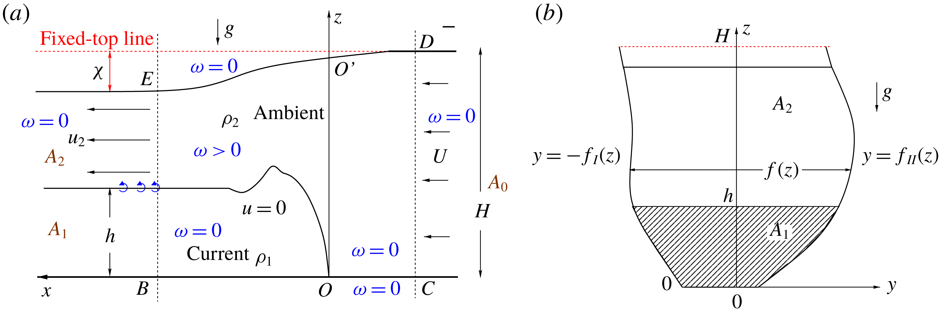
The analysis is performed in a Cartesian coordinate system attached to the current (see figure 3). The
 $x$
axis is in the direction of the flow of the less dense fluid (the ambient), and the origin
 $O$
is at the leading edge of the current, which is a stagnation point for the ambient fluid. We emphasize that the upper surface and interface are flat (horizontal) in the lateral direction
 $y$
.
The c.v. attached to the current. The upper boundary is open to the atmosphere
 $p=0$
. Parameter
 $\unicode[STIX]{x1D714}$
(
 $y$
component of vorticity) is
 $0$
on the boundary of the c.v. except for the vortex sheet (
 $\circlearrowleft$
) at the interface
 $z=h$
. The sketched values of
 $\unicode[STIX]{x1D714}$
inside the c.v. are expected. Here
 $A_{0},A_{1}$
and
 $A_{2}$
denote the cross-section area of the domain.

We use a c.v. with vertical boundaries denoted
 $CD$
in the upstream and
 $BE$
in the downstream sides. The fluids differ sharply in density,
 $\unicode[STIX]{x1D70C}_{1}>\unicode[STIX]{x1D70C}_{2}$
, and the ‘interface’ describes this separation. The velocity (in the
 $x$
direction) of the light fluid upstream is
 $U$
and downstream is
 $u_{2}$
. In the c.v. attached to the current, the dense fluid is assumed motionless,
 $u_{1}=0$
. The
 $y$
component of the vorticity is denoted by
 $\unicode[STIX]{x1D714}$
.
The conditions on the boundary of the c.v. are as follows. The upstream flow (over the entire
 $A_{0}$
) has uniform velocity
 $U$
and hence is irrotational. The downstream flow is again horizontal with
 $u_{2}=$
const. and irrotational over
 $A_{2}$
(except for an infinitesimal layer at
 $z=h$
as specified below). On the bottom, top and side boundaries of the c.v. there is no penetration and free slip, which implies no shear and zero vorticity. At the interface
 $z=h$
there is continuity of pressure, and a very (infinitesimally) thin vortex sheet in which
 $u_{2}$
develops from
 $0$
and a large
 $\unicode[STIX]{x1D714}=\unicode[STIX]{x2202}u/\unicode[STIX]{x2202}z$
is present. The free-slip boundary condition is a rigorous theoretical condition for the Navier–Stokes equation, and can be straightforwardly assigned in numerical simulations. However, in realistic systems this is an approximation. At the open top a free-slip condition is evidently a good approximation. For the bottom solid wall we employ the argument that at large
 $Re$
the viscous forces at the boundary are small as compared to pressure and inertia force of the control volume. Then, considering the flow-force equation, we argue that the use of the free-slip approximation introduces an error
 $O(1/Re)$
in the calculation of
 $Fr^{2}$
. A sharp evaluation of this error is, to our knowledge, unavailable. We emphasize that the free-slip condition is an essential ingredient in Benjamin’s analysis, and hence our study adopts this assumption also as a part of a starting-point model. We are concerned with relaxing two assumptions of Benjamin: 2D flow and a fixed-top boundary. We note that, implicitly, by relaxing the fixed-top assumptions, we also improve the relevance of the free-slip assumption of Benjamin.
We do not specify the flow of the ambient fluid inside the c.v. However, some qualitative features that are physically consistent with the foregoing assumption must be taken into account. At the line
 $x=0$
(represented by point
 $O$
in figure 3
a) the ambient fluid encounters an obstacle which deflects the streamlines, most strongly in the domain of the head of the current whose expected shape is sketched in the figure. The interface (between the current and the ambient) may, in general, contribute shear and generate vorticity, which in turn may affect the dynamics of the fluid which flows over the head of the current. The velocity
 $\boldsymbol{v}$
in this domain is three-dimensional with components
 $\{u,v,w\}$
functions of
 $x,y,z$
, and a non-zero vorticity
 $\unicode[STIX]{x1D735}\times \boldsymbol{v}$
may appear, whose
 $y$
component is
 $\unicode[STIX]{x1D714}=\unicode[STIX]{x2202}u/\unicode[STIX]{x2202}z-\unicode[STIX]{x2202}w/\unicode[STIX]{x2202}x$
. (Unlike the top and bottom boundaries where free-slip conditions may be imposed, the interface is an internal component of the two-fluid system which couples between the upper and lower fluids inside the control volume.) Therefore, although the upstream flow is irrotational and energy-conserving, in the c.v., while being contracted by the current-head obstacle, the ambient fluid is, in general, affected by vorticity effects and dissipates energy. In the downstream domain (to the left of the
 $EB$
boundary) the flow is again parallel-irrotational, but the net effect of the interaction with the head remains: there is headloss on all the streamlines that have crossed from right to left, and a vorticity sheet is present along the interface. Note, however, that a particle on the
 $CO$
streamline
 $(x<0)$
cannot be affected by either diffusion or convection from the interface at
 $x>0$
, and hence the entire kinetic energy at
 $C$
is converted into stagnation pressure at
 $O$
, the headloss on the other streamlines notwithstanding. As pointed out by Benjamin (Reference Benjamin1968), these non-ideal-fluid effects inside the c.v., not introduced explicitly, are essential to the flow of realistic GCs. The GC model is an emulation of the Navier–Stokes equation with free-slip boundary condition on the walls, not of the perfect-fluid Euler equations. Attempts to impose inviscid energy-conserving conditions in the c.v. reduce the applicability of the
 $Fr$
result to special values of
 $a$
. This observation is valid also for the present problem, as shown below.
For the convenience of the reader, we recall the definitions
 $$\begin{eqnarray}a=\frac{h}{H};\quad r=\frac{\unicode[STIX]{x1D70C}_{2}}{\unicode[STIX]{x1D70C}_{1}};\quad \unicode[STIX]{x0394}\unicode[STIX]{x1D70C}=\unicode[STIX]{x1D70C}_{1}-\unicode[STIX]{x1D70C}_{2};\quad \unicode[STIX]{x1D716}\,=\frac{\unicode[STIX]{x0394}\unicode[STIX]{x1D70C}}{\unicode[STIX]{x1D70C}_{2}};\quad g^{\prime }=\unicode[STIX]{x1D716}\,g;\quad Fr=\frac{U}{(g^{\prime }h)^{1/2}};\quad \tilde{\unicode[STIX]{x1D712}}=\frac{\unicode[STIX]{x1D712}}{H}.\end{eqnarray}$$
The task is to derive
 $Fr(a,r)$
and
 $\tilde{\unicode[STIX]{x1D712}}(a,r)$
solutions, and determine the range of validity,
 $a\in (0,a_{max}(r)\!]$
. By
 $a=0$
we mean the limit of a current of finite
 $h$
which is thin, or deep, compared with
 $H$
,
 $(h/H)\rightarrow 0$
. It is convenient to denote the area and the pressure of the upstream unperturbed domain by the subscript
 $0$
. In the downstream domain we use the more obvious subscripts 1, 2 for the lower and upper fluids.
2.1 Hydrostatic pressure
The assumed boundary conditions reduce the vertical component of the Navier–Stokes equations in the upstream and downstream domains to the hydrostatic pressure balances
 $\unicode[STIX]{x2202}p/\unicode[STIX]{x2202}z=-\unicode[STIX]{x1D70C}_{i}g$
. With the
 $p=0$
condition at top, and continuity at the interface
 $z=h$
in the downstream side, the resulting pressure field is
 $$\begin{eqnarray}\displaystyle & \displaystyle \text{upstream:}\quad p_{0}(z)=\unicode[STIX]{x1D70C}_{2}g(H-z)\quad \text{over }A_{0} & \displaystyle\end{eqnarray}$$
 $$\begin{eqnarray}\displaystyle & \displaystyle \text{downstream:}\quad p=\left\{\begin{array}{@{}ll@{}}p_{2}(z)=\unicode[STIX]{x1D70C}_{2}g(H-\unicode[STIX]{x1D712}-z) & \text{over }A_{2}\\ p_{1}(z)=\unicode[STIX]{x1D70C}_{2}g(H-\unicode[STIX]{x1D712}-z)+\unicode[STIX]{x0394}\unicode[STIX]{x1D70C}g(h-z) & \text{over }A_{1}.\end{array}\right. & \displaystyle\end{eqnarray}$$
2.2 Pressure loop; the first
 $Fr,\tilde{\unicode[STIX]{x1D712}}$
relationship

Since the pressure is a single-valued function, the hydrostatic upstream and downstream pressure results are components of a closed circuit. In particular, the pressure at
 $B$
calculated from upstream along the
 $DCOB$
path must be equal to the value obtained along
 $EB$
.
Consistent with Benjamin’s analysis,
 $O$
is a perfect stagnation point (i.e. there is no headloss; the justification is given in Ungarish (Reference Ungarish2017)). We thus write the Bernoulli balance on
 $BOC$
using (2.2) at
 $z=0$
:
 $$\begin{eqnarray}p_{B}=p_{O}={\textstyle \frac{1}{2}}\unicode[STIX]{x1D70C}_{2}U^{2}+\unicode[STIX]{x1D70C}_{2}gH.\end{eqnarray}$$
On the other hand,
 $p_{B}=p_{1}(z=0)$
given by (2.3). Matching the values we obtain
 $$\begin{eqnarray}\unicode[STIX]{x1D712}=\frac{\unicode[STIX]{x0394}\unicode[STIX]{x1D70C}}{\unicode[STIX]{x1D70C}_{2}}h-\frac{1}{2}\frac{U^{2}}{g}.\end{eqnarray}$$
In dimensionless form, using the definitions in (2.1), this is expressed as
 $$\begin{eqnarray}\tilde{\unicode[STIX]{x1D712}}=\unicode[STIX]{x1D716}\,a\left(1-{\textstyle \frac{1}{2}}Fr^{2}\right);\quad \text{or}\quad \unicode[STIX]{x1D712}/h=\unicode[STIX]{x1D716}\,\left(1-{\textstyle \frac{1}{2}}Fr^{2}\right).\end{eqnarray}$$
This is a fundamental relationship in our analysis. It provides an explicit dependency, the ‘first equation’, between the unknown quantities
 $\tilde{\unicode[STIX]{x1D712}},Fr$
. As expected, the height reduction of the open surface is significant only for non-Boussinesq, non-deep currents (
 $\unicode[STIX]{x1D716}\,$
and
 $a$
not very small). We restrict the investigation to positive
 $\unicode[STIX]{x1D712}$
, i.e. the open surface dips over the current. We note that a negative
 $\unicode[STIX]{x1D712}$
is formally possible, but this is associated with high-speed flows with
 $Fr^{2}>2$
, which are expected to be in the problematic supercritical (with respect to the internal shallow-water waves, or characteristics) regime, as briefly discussed in appendix A. Moreover, the generation of a current with large speed may require an energy source, which is not expected in common circumstances.
2.3 Volume and
$x$
-momentum balance; the second
$Fr,\tilde{\unicode[STIX]{x1D712}}$
equation


The volume balance is
 $$\begin{eqnarray}A_{0}U=A_{2}u_{2}.\end{eqnarray}$$
Since there are no
 $x$
-shear forces on the c.v. envelope, the global (over the c.v.)
 $x$
-momentum balance is between momentum flux and pressure force. This can be expressed, using (2.2)–(2.3), as
 $$\begin{eqnarray}\displaystyle \unicode[STIX]{x1D70C}_{2}A_{0}U(u_{2}-U) & = & \displaystyle \int _{A_{0}}p_{0}\,\text{d}A-\left(\int _{A_{1}}p_{1}\,\text{d}A+\int _{A_{2}}p_{2}\,\text{d}A\right)\nonumber\\ \displaystyle & = & \displaystyle \unicode[STIX]{x1D70C}_{2}g\left[\int _{A_{0}-A_{1}-A_{2}}(H-z)\,\text{d}A+\unicode[STIX]{x1D712}(A_{1}+A_{2})-\unicode[STIX]{x1D716}\,\int _{A_{1}}(h-z)\,\text{d}A\right]\!.\quad\end{eqnarray}$$
The reduction of the force term follows from the observation that
 $p_{0},-p_{1},-p_{2}$
share the
 $H-z$
term, while
 $p_{1},p_{2}$
share the
 $-\unicode[STIX]{x1D712}$
term. In the momentum flux term we eliminate
 $u_{2}$
with the aid of (2.7), then replace
 $U^{2}$
with
 $\unicode[STIX]{x1D716}\,gFr^{2}h$
, rewrite the area integrals in a more explicit form and obtain the ‘second equation’ of our problem
 $$\begin{eqnarray}\left(\frac{A_{0}}{A_{2}}-1\right)Fr^{2}=\frac{1}{\displaystyle \unicode[STIX]{x1D716}\,hA_{0}}\int _{H-\unicode[STIX]{x1D712}}^{H}(H-z)f(z)\,\text{d}z+\left(\frac{\unicode[STIX]{x1D712}}{\unicode[STIX]{x1D716}\,h}\right)\frac{A_{1}+A_{2}}{A_{0}}-\frac{A_{1}}{A_{0}}+\frac{1}{\displaystyle hA_{0}}\int _{0}^{h}zf(z)\,\text{d}z,\end{eqnarray}$$
which must be solved together with the fundamental ‘first equation’ (2.6) (repeated)
 $$\begin{eqnarray}\unicode[STIX]{x1D712}=\unicode[STIX]{x1D716}\,h\left(1-{\textstyle \frac{1}{2}}Fr^{2}\right);\quad \text{or}\quad \tilde{\unicode[STIX]{x1D712}}=\unicode[STIX]{x1D716}\,a\left(1-{\textstyle \frac{1}{2}}Fr^{2}\right).\end{eqnarray}$$
A useful simplification is attained by substituting (2.10) into the second term of the right-hand side of (2.9), and rearranging into
 $$\begin{eqnarray}\left[\frac{A_{0}}{A_{2}}-1+\frac{1}{2}\frac{A_{1}+A_{2}}{A_{0}}\right]Fr^{2}=\frac{A_{2}}{A_{0}}+\frac{1}{\displaystyle \unicode[STIX]{x1D716}\,hA_{0}}\int _{H-\unicode[STIX]{x1D712}}^{H}(H-z)f(z)\,\text{d}z+\frac{1}{\displaystyle hA_{0}}\int _{0}^{h}zf(z)\,\text{d}z.\end{eqnarray}$$
This result is of the form
 $P(\tilde{\unicode[STIX]{x1D712}})Fr^{2}-Q(\tilde{\unicode[STIX]{x1D712}})-J=0$
, where the functions
 $P$
,
 $Q$
and
 $J$
depend on
 $f$
, and thus justifies the name ‘second equation’ for the
 $Fr$
and
 $\tilde{\unicode[STIX]{x1D712}}$
variables. (Another convenient form of the ‘second equation’ is (2.17), as shown below.)
For given
 $f(z),H$
and
 $h$
the equations (2.10)–(2.11) provide a system for
 $Fr^{2}$
and
 $\unicode[STIX]{x1D712}$
(or
 $\tilde{\unicode[STIX]{x1D712}}$
) amenable for solution by iterations: guess
 $Fr$
, calculate
 $\unicode[STIX]{x1D712}$
by (2.10), check the balance (2.11); correct
 $Fr$
, etc. Note that
 $A_{0}$
,
 $A_{1}$
and the last term of (2.11) remain constant during the iterations. Similar problems suggest that
 $Fr=1$
is a convenient starting point. Formally, elimination of
 $\unicode[STIX]{x1D712}$
by (2.10) renders (2.11) as a single equation for
 $Fr^{2}$
, but we found no advantage in this step. Assuming that the iterations converge to some apparently acceptable solution with positive
 $Fr,\tilde{\unicode[STIX]{x1D712}}$
, we focus our attention on the domain of validity.
2.4 Energy dissipation and range of validity
An important observation of Benjamin (Reference Benjamin1968) is that the propagation of a steady-state GC is in general not an energy-conserving process, and hence the validity of the c.v. solution is restricted to the domain where the headloss (dissipation) is non-negative. For the relevant test, consider Bernoulli’s balance on the streamline
 $DE$
in figure 3, where
 $p=0$
and the speed increases from
 $U$
to
 $u_{2}$
. For generality, in accord with Benjamin’s methodology, we allow headloss
 $\unicode[STIX]{x1D70C}_{2}g^{\prime }\unicode[STIX]{x1D6FF}_{t}$
(the subscript means top), to write
 $u_{2}^{2}/2-g\unicode[STIX]{x1D712}=U^{2}/2-g^{\prime }\unicode[STIX]{x1D6FF}_{t}$
. Combining with (2.5) we obtain
 $$\begin{eqnarray}{\textstyle \frac{1}{2}}u_{2}^{2}=g^{\prime }h-g^{\prime }\unicode[STIX]{x1D6FF}_{t},\end{eqnarray}$$
which combined with (2.7) reads
 $$\begin{eqnarray}\frac{\unicode[STIX]{x1D6FF}_{t}}{h}=1-\frac{1}{2}Fr^{2}\left(\frac{A_{0}}{A_{2}}\right)^{2}.\end{eqnarray}$$
Since
 $u_{2}$
is
 $z$
-independent, the same headloss results for all the streamlines (or streamtubes) of the ambient fluid (the only exception is the stagnation streamline
 $CO$
). Therefore the total rate of dissipation of the system is
 $$\begin{eqnarray}\dot{{\mathcal{D}}}=\unicode[STIX]{x1D70C}_{2}g^{\prime }\unicode[STIX]{x1D6FF}_{t}A_{0}U=\unicode[STIX]{x1D70C}_{2}(g^{\prime }h)^{3/2}A_{0}Fr\left[1-\frac{1}{2}Fr^{2}\left(\frac{A_{0}}{A_{2}}\right)^{2}\right].\end{eqnarray}$$
The
 $\dot{{\mathcal{D}}}=0$
situation corresponds to an energy-conserving current. Solutions with negative
 $\dot{{\mathcal{D}}}$
(and
 $\unicode[STIX]{x1D6FF}_{t}$
) are considered energetically invalid, and will be discarded. Using (2.14), the validity criterion
 $\dot{{\mathcal{D}}}\geqslant 0$
is expressed as
 $$\begin{eqnarray}Fr\leqslant \sqrt{2}\frac{A_{2}}{A_{0}}.\end{eqnarray}$$
The energy-conserving (non-dissipative) system corresponds to the equality sign in (2.15). In this case we have three equations (energy conservation plus (2.9) and (2.10)) for the variables
 $\tilde{\unicode[STIX]{x1D712}}$
and
 $Fr$
, and hence a solution exists only for some special cases, when
 $a=a_{max}(r)$
. Note that systems with small
 $a$
and
 $\tilde{\unicode[STIX]{x1D712}}$
display
 $A_{2}/A_{0}$
close to 1, and thus satisfy the validity criterion (2.15) for
 $Fr<\sqrt{2}$
. As
 $a$
increases,
 $A_{2}$
becomes smaller, and the right-hand side of (2.15) becomes more restrictive. This justifies the formulation of the energy dissipation restriction as
 $a\leqslant a_{max}(r)$
, where
 $a_{max}$
corresponds to the energy-conserving current. The solutions considered below confirm this inference.
The presence of a
 $z$
-independent headloss
 $\unicode[STIX]{x1D6FF}_{t}$
for all the streamlines in the
 $z>h$
domain, including the top
 $DE$
, is a problematic point of the model, in particular for a shallow current with small
 $a$
. Physical considerations and Navier–Stokes simulation (e.g. Borden & Meiburg Reference Borden and Meiburg2013) indicate that in a real flow the vorticity and dissipation effects which develop inside the control volume are left behind (outfluxed from
 $EB$
in figure 3) in a layer (wake) of small but finite thickness about the ideal
 $z=h$
interface between the current and the ambient. The use of this observation in a simple mathematical model for the prediction of
 $Fr$
and the range of validity is still open to interpretations. This topic has been addressed by several studies of the 2D geometry, as reviewed in a recent paper (Ungarish & Hogg Reference Ungarish and Hogg2018). In particular, the recent circulation-based models (e.g. Borden & Meiburg Reference Borden and Meiburg2013, Baines Reference Baines2016) emphasized the concentration of the vorticity in a vortex-sheet layer. However, since the vortex sheet carries no volume, this component cannot reproduce the rate of dissipation of the jump, and hence in this model the dissipation must also be distributed in the streamlines above the sheet. Indeed, the flow derived in Borden & Meiburg (Reference Borden and Meiburg2013) has in general a non-zero
 $\unicode[STIX]{x1D6FF}_{t}$
like Benjamin’s model (see figure 6 in that paper).
To model the presence of dissipation only in the layer close to the interface, it is necessary to relax the constant
 $u_{2}$
assumption, and allow a transition layer of finite thickness. The mixing-layer model (Borden, Meiburg & Constantinescu Reference Borden, Meiburg and Constantinescu2012; Baines Reference Baines2016) needs some empirical, or semi-empirical, closures for the thickness of the layer. The vortex-wake model (Ungarish Reference Ungarish2017, Ungarish & Hogg Reference Ungarish and Hogg2018) needs an assumption about the profile
 $u_{2}(z)$
. For the finite-thickness (wake)
 $u_{2}(z)$
profile, the continuity, momentum and energy balances are more complicated and less insightful than for the vortex-sheet model with constant
 $u_{2}$
. The tests performed for the 2D geometry demonstrate that the use of a more realistic
 $u_{2}(z)$
profile renders very similar values of
 $Fr$
and exactly the same range of validity as the simpler Benjamin model. The interpretation is that the end results of the c.v. analysis are integrals that smooth out the local behaviour. When integrated over the outflow boundary of the c.v., the contributions of constant and
 $z$
-dependent
 $u_{2}$
and headloss yield very similar results.
For the open-surface 2D case, consider figures 3–5(a) of Ungarish (Reference Ungarish2017) which show the results of the vortex-sheet and vortex-wake models; we note that the major results of
 $Fr,\tilde{\unicode[STIX]{x1D712}}$
, and range of validity, are (almost) identical for the entire parameter range relevant to the problem. We argue that this agreement, or compatibility, between the models is expected to carry over also to the GCs with non-rectangular cross-sections considered in this paper. The justification is as given above:
 $Fr$
and
 $\tilde{\unicode[STIX]{x1D712}}$
represent some integral balances over the boundaries of the c.v., and the integration smooths out the
 $z$
-dependent details of the headloss distribution. We therefore use here the simple model with constant
 $u_{2}$
in the ambient (the detailed calculations for the vortex-wake model are formally possible, but cumbersome, and were not attempted in the present work). As a result of this simplification, at the downstream boundary the vorticity is concentrated in a vortex sheet, and the dissipation is distributed homogeneously. We reiterate that these are simplifications of the model, not an accurate representation of details of the flow field. The justification of this simplification is the evidence that in closely related flow fields the use of more realistic (and more complicated)
 $u_{2}$
profiles yields very similar
 $Fr$
and
 $\tilde{\unicode[STIX]{x1D712}}$
results. A more stringent justification requires comparisons with high-resolution Navier–Stokes simulations, which must be left to future work.
We note in passing that the left-hand side of (2.12) is the integral of
 $u(\unicode[STIX]{x2202}u/\unicode[STIX]{x2202}z)$
with respect to
 $z$
on the downstream boundary, from
 $u=u_{1}=0$
to
 $u_{2}$
. Therefore the left-hand side of (2.12) can be interpreted as the flux of vorticity
 $\unicode[STIX]{x1D714}=(\unicode[STIX]{x2202}u/\unicode[STIX]{x2202}z)$
in the vortex sheet about
 $z=h$
. There is no other inflow or outflow of
 $\unicode[STIX]{x1D714}$
on the boundaries of the c.v. Therefore, equation (2.12) is, implicitly, the balance of vorticity of the flow (per unit width, multiply by
 $f(h)$
for the total): while the right-hand side term gives the net outflux from the control volume along the vortex sheet, the terms on the right-hand side represent the baroclinic torque and vorticity diffusion which pertain to the c.v. domain. In other words, the vorticity balance of the flow is implicitly included in our formulation. Note that the continuous change of the ambient velocity from
 $0$
to the constant
 $u_{2}$
in the thin vortex sheet implies a viscous effect at the interface.
2.5 The limits of Boussinesq, and deep current
Before proceeding to a general solution, it is insightful to consider the behaviour for two important limiting cases:
 $\unicode[STIX]{x1D716}\,\rightarrow 0$
and
 $a\rightarrow 0$
.
An inspection of (2.10)–(2.11) suggests some rearrangement. First, we define
 $\unicode[STIX]{x1D701}=H-z$
, recall
 $\unicode[STIX]{x1D712}=\tilde{\unicode[STIX]{x1D712}}H$
and rewrite the second term on the right-hand side of (2.11) as
 $$\begin{eqnarray}G=\frac{1}{\displaystyle \unicode[STIX]{x1D716}\,hA_{0}}\int _{H-\unicode[STIX]{x1D712}}^{H}(H-z)f(z)\,\text{d}z=\left(\frac{\unicode[STIX]{x1D712}}{\unicode[STIX]{x1D716}\,h}\right)\tilde{\unicode[STIX]{x1D712}}\underbrace{\left[\frac{H}{\unicode[STIX]{x1D712}^{2}A_{0}}\int _{0}^{\unicode[STIX]{x1D712}}\unicode[STIX]{x1D701}f(H-\unicode[STIX]{x1D701})\,\text{d}\unicode[STIX]{x1D701}\right]}_{B}=\left(1-\frac{1}{2}Fr^{2}\right)B\tilde{\unicode[STIX]{x1D712}}.\end{eqnarray}$$
We used (2.10) to replace the term
 $\unicode[STIX]{x1D712}/(\unicode[STIX]{x1D716}\,h)$
, and defined
 $B$
as the term in the brackets. We note that in general
 $B$
is of the order of unity (a straightforward approximation for the integral is
 $\unicode[STIX]{x1D712}^{2}f(H)/2$
for small
 $\tilde{\unicode[STIX]{x1D712}}$
). The result (2.16) allows the distribution of
 $G$
between the sides of (2.11) to yield
 $$\begin{eqnarray}\left[\frac{A_{0}}{A_{2}}-1+\frac{1}{2}\frac{A_{1}+A_{2}}{A_{0}}+\frac{1}{2}B\tilde{\unicode[STIX]{x1D712}}\right]Fr^{2}=\frac{A_{2}}{A_{0}}+B\tilde{\unicode[STIX]{x1D712}}+\frac{1}{\displaystyle hA_{0}}\int _{0}^{h}zf(z)\,\text{d}z.\end{eqnarray}$$
We repeat the fundamental and energy restriction equations
 $$\begin{eqnarray}\quad \tilde{\unicode[STIX]{x1D712}}=\unicode[STIX]{x1D716}\,a\left(1-\frac{1}{2}Fr^{2}\right);\quad Fr^{2}\leqslant 2\left(\frac{A_{2}}{A_{0}}\right)^{2}.\end{eqnarray}$$
Let
 $\unicode[STIX]{x1D711}=A_{1}/A_{0}$
. Consider the situation
 $\unicode[STIX]{x1D712}\rightarrow 0$
. In this limit,
 $A_{1}+A_{2}=A_{0}$
and
 $A_{2}/A_{0}=1-\unicode[STIX]{x1D711}$
. The
 $B\tilde{\unicode[STIX]{x1D712}}$
terms in (2.17) vanish, and we obtain
 $$\begin{eqnarray}Fr^{2}=2\frac{1-\unicode[STIX]{x1D711}}{1+\unicode[STIX]{x1D711}}\left[1-\unicode[STIX]{x1D711}+\frac{1}{\displaystyle hA_{0}}\int _{0}^{h}zf(z)\,\text{d}z\right]\quad (\tilde{\unicode[STIX]{x1D712}}\rightarrow 0).\end{eqnarray}$$
This limit coincides with the formula
 $Fr_{f}$
derived for the current in a channel with fixed top (see (1.2)). The energy conditions (2.18b
), for
 $A_{2}/A_{0}=1-\unicode[STIX]{x1D711}$
, also reduce to
 $[Fr/(1-\unicode[STIX]{x1D711})]^{2}\leqslant 2$
like in the fixed-top case. This agreement is relevant in two open-surface cases:
(1) The Boussinesq limit. It is evident that for a finite
$a=h/H$
, when
$\unicode[STIX]{x1D716}\,\rightarrow 0$
(i.e.
$r\rightarrow 1$
) we obtain
$\tilde{\unicode[STIX]{x1D712}}\rightarrow 0$
(see (2.18a
)). The Boussinesq open-top currents attain the same
$Fr$
, energy and critical-speed values as the fixed-top counterpart.(2) The very thin current limit. Consider
$a\rightarrow 0$
while
$\unicode[STIX]{x1D716}\,$
is finite. We infer that
$\tilde{\unicode[STIX]{x1D712}}\rightarrow 0$
, because this case (
$a\rightarrow 0,\tilde{\unicode[STIX]{x1D712}}\rightarrow 0$
) corresponds to
$Fr^{2}=2$
by (2.19). On the other hand, equation (2.18a
) confirms that for
$Fr^{2}\rightarrow 2$
and fixed
$\unicode[STIX]{x1D716}\,$
we obtain
$\tilde{\unicode[STIX]{x1D712}}\rightarrow 0$
. This justifies the conclusion that a very thin (deep) current will display the same
$Fr^{2}=2$
and dissipation in open- and fixed-top systems. The robustness of the deep-current result
$Fr^{2}=2$
is remarkable. It was first derived for the 2D current by Kármán (Reference Kármán1940), then by Benjamin (Reference Benjamin1968), and appears again and again in various solutions (e.g. Klemp et al.
Reference Klemp, Rotunno and Skamarock1994, Ungarish Reference Ungarish2006, Borden & Meiburg Reference Borden and Meiburg2013, Milewski & Tabak Reference Milewski and Tabak2015), including the present one.


We also note that the
 $\unicode[STIX]{x1D716}\,\rightarrow \infty$
(
 $r\rightarrow 0$
) limit of the
 $Fr,\unicode[STIX]{x1D712}$
formulation is ill-posed. The physical interpretation is that in the absence of a fluid of finite density between the open surface and the current the two-layer balance equations are ambiguous.
2.6 Summary
This ends the formulation. We derived a system of two fairly simple coupled algebraic equations (2.10)–(2.11) (or (2.10) and (2.17)) for the variables
 $Fr$
and
 $\tilde{\unicode[STIX]{x1D712}}$
, as functions of
 $a=h/H$
and the density parameter
 $r$
(or
 $\unicode[STIX]{x1D716}\,=1/r-1$
); the geometry of the cross-section of the channel enters via the width function
 $f(z)$
. The headloss and dissipation rate of the flow are obtained explicitly from the auxiliary equations (2.13) and (2.14). The validity of the result is easily determined by (2.15). (The critical speed criterion can also be evaluated if needed; see appendix A.)
The formulation yields in general a strongly nonlinear system, and it is not clear a priori that acceptable solutions exist, except for the previously published 2D (rectangular) cross-section case (Ungarish Reference Ungarish2017). The relevance to more general geometries is indicated by two limiting cases (see § 2.5): in the Boussinesq case (
 $r\rightarrow 1$
or
 $\unicode[STIX]{x1D716}\,\rightarrow 0$
), the present formulation recovers the fixed-top results; and for a very thin current
 $a\rightarrow 0$
, fixed
 $r$
, the present theory predicts
 $Fr=\sqrt{2},\tilde{\unicode[STIX]{x1D712}}=0$
.
The implementation to some additional practical cases is illustrated below.
3 Solutions
It is insightful to consider detailed solutions and comparison for the following cross-section cases: (i) power-law
 $f(z)=bz^{\unicode[STIX]{x1D6FC}}$
; and (ii) trapezoid
 $f(z)=H-\unicode[STIX]{x1D6FD}z$
.
The power-law cross-section
 $f(z)=bz^{\unicode[STIX]{x1D6FC}}$
, where
 $b>0,\unicode[STIX]{x1D6FC}\geqslant 0$
are constants, is considered for
 $\unicode[STIX]{x1D6FC}=0$
,
 $1/2$
and
 $1$
, which correspond to a rectangle (2D case), semi-circle (approximation valid when
 $H$
is smaller than the radius) and triangle. The rectangle is used for reference, while the profiles with
 $\unicode[STIX]{x1D6FC}>0$
highlight the influence of an expanding (with
 $z$
) cross-section. The trapezoid with
 $\unicode[STIX]{x1D6FD}=0.5$
highlights the influence of a contracting (with
 $z$
) cross-section.
Some details are as follows. For the power-law case,
 $A_{0}=bH^{\unicode[STIX]{x1D6FC}+1}/(\unicode[STIX]{x1D6FC}+1),A_{1}=bh^{\unicode[STIX]{x1D6FC}+1}/(\unicode[STIX]{x1D6FC}+1),A_{2}=b[(H-\unicode[STIX]{x1D712})^{\unicode[STIX]{x1D6FC}+1}-h^{\unicode[STIX]{x1D6FC}+1}]/(\unicode[STIX]{x1D6FC}+1)$
. The evaluation of the integrals in the right-hand side of (2.11) is straightforward, and after some algebra we obtain
 $$\begin{eqnarray}\left[\frac{1}{\displaystyle (1-\tilde{\unicode[STIX]{x1D712}})^{\unicode[STIX]{x1D6FC}+1}-a^{\unicode[STIX]{x1D6FC}+1}}-1+\frac{1}{2}(1-\tilde{\unicode[STIX]{x1D712}})^{\unicode[STIX]{x1D6FC}+1}\right]Fr^{2}=(1-\tilde{\unicode[STIX]{x1D712}})^{\unicode[STIX]{x1D6FC}+1}+G-\frac{a^{\unicode[STIX]{x1D6FC}+1}}{\unicode[STIX]{x1D6FC}+2},\end{eqnarray}$$
where
 $$\begin{eqnarray}G=\frac{1}{\displaystyle \unicode[STIX]{x1D6FC}+2}\frac{1}{\displaystyle \unicode[STIX]{x1D716}\,a}\left[1-(1-\tilde{\unicode[STIX]{x1D712}})^{\unicode[STIX]{x1D6FC}+1}[1+(\unicode[STIX]{x1D6FC}+1)\tilde{\unicode[STIX]{x1D712}}]\right]=\frac{\unicode[STIX]{x1D6FC}+1}{2}\left(\frac{\tilde{\unicode[STIX]{x1D712}}}{\unicode[STIX]{x1D716}\,a}\right)\tilde{\unicode[STIX]{x1D712}}[1-O(\unicode[STIX]{x1D6FC}\tilde{\unicode[STIX]{x1D712}})].\end{eqnarray}$$
The expansion for small
 $\tilde{\unicode[STIX]{x1D712}}$
in the last term of (3.2) indicates that
 $G=0$
for
 $\tilde{\unicode[STIX]{x1D712}}\rightarrow 0$
. Note that the leading term contains the coefficient
 $\tilde{\unicode[STIX]{x1D712}}/(\unicode[STIX]{x1D716}\,a)$
which can be eliminated by (2.10).
For
 $\unicode[STIX]{x1D6FC}=0$
the present formulation recovers the 2D results reported in Ungarish (Reference Ungarish2017).
For
 $\unicode[STIX]{x1D6FC}=1$
we obtain the
 $\vee$
triangle
 $f(z)=z$
. Equation (3.1) reduces to
 $$\begin{eqnarray}\left[\frac{1}{\displaystyle (1-\tilde{\unicode[STIX]{x1D712}})^{2}-a^{2}}-1+\frac{1}{2}(1-\tilde{\unicode[STIX]{x1D712}})^{2}\right]Fr^{2}=(1-\tilde{\unicode[STIX]{x1D712}})^{2}+\frac{\tilde{\unicode[STIX]{x1D712}}}{\unicode[STIX]{x1D716}\,a}\tilde{\unicode[STIX]{x1D712}}(1-(2/3)\tilde{\unicode[STIX]{x1D712}})-\frac{1}{\displaystyle 3}a^{2}.\end{eqnarray}$$
Elimination of
 $\tilde{\unicode[STIX]{x1D712}}$
by (2.10) is not beneficial even in this case, because it produces a fifth-order equation for
 $Fr^{2}$
.
For the trapezoidal
 $f(z)=H-\unicode[STIX]{x1D6FD}z$
cross-section,
 $\unicode[STIX]{x1D6FD}<1$
, the calculation of
 $A_{0,1,2}$
and the other needed integrals is simple. We present results for
 $\unicode[STIX]{x1D6FD}=0.5$
. This is an upward-narrowing (converging) cross-section, in contrast to the upward-enlarging (diverging) power law profiles considered above.
Plots of
 $Fr$
and
 $\tilde{\unicode[STIX]{x1D712}}$
versus
 $r$
for various
 $a$
in range of validity. Here
 $f(z)$
is a power law with specified
 $\unicode[STIX]{x1D6FC}$
or trapezoid with specified
 $\unicode[STIX]{x1D6FD}$
.

Plots of
 $Fr/Fr_{f}(a)$
versus
 $r$
for various
 $a$
in range of validity.

To summarize, our open-top system examples essentially consider
 $\vee$
shapes versus
 $\text{}\underline{/~\backslash }$
shapes, with the rectangle in between. The reported
 $Fr$
and
 $\tilde{\unicode[STIX]{x1D712}}$
values were obtained by iteration. We used the secant method to obtain convergence of about ten digits. The results are presented in figures 4–7.
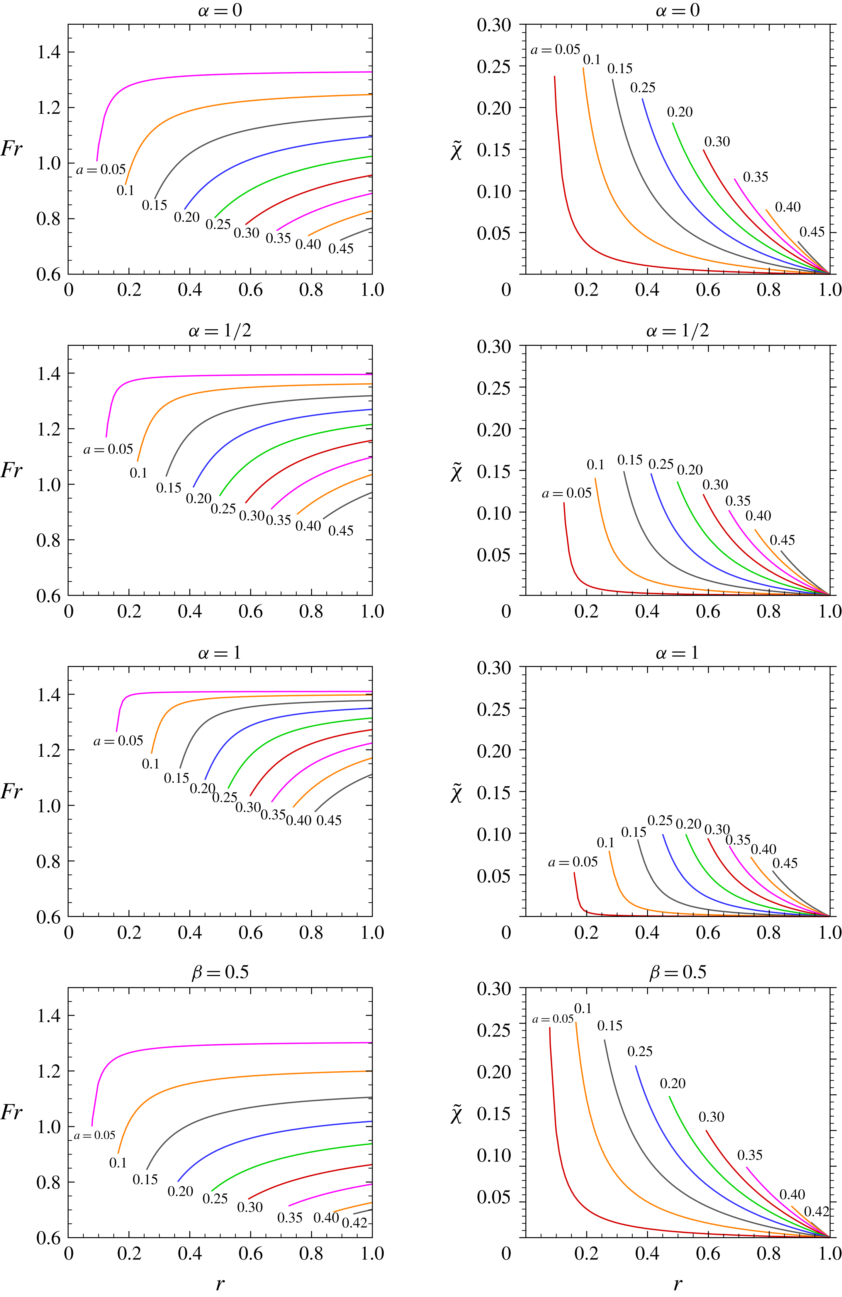
Figure 4 presents the
 $Fr$
and
 $\tilde{\unicode[STIX]{x1D712}}$
results for four different
 $f(z)$
(from top to bottom): rectangle, semi-circle,
 $\vee$
triangle and
 $\text{}\underline{/~\backslash }$
trapezoid. The lines are for fixed values of
 $a=h/H$
. The displayed values are energetically valid; therefore, each line terminates at the
 $r$
position where the energy-conserving point (equality sign of (2.15)) is attained. For smaller
 $r$
, the
 $Fr,\tilde{\unicode[STIX]{x1D712}}$
results yield a negative
 $\unicode[STIX]{x1D6FF}_{t}$
in (2.13).
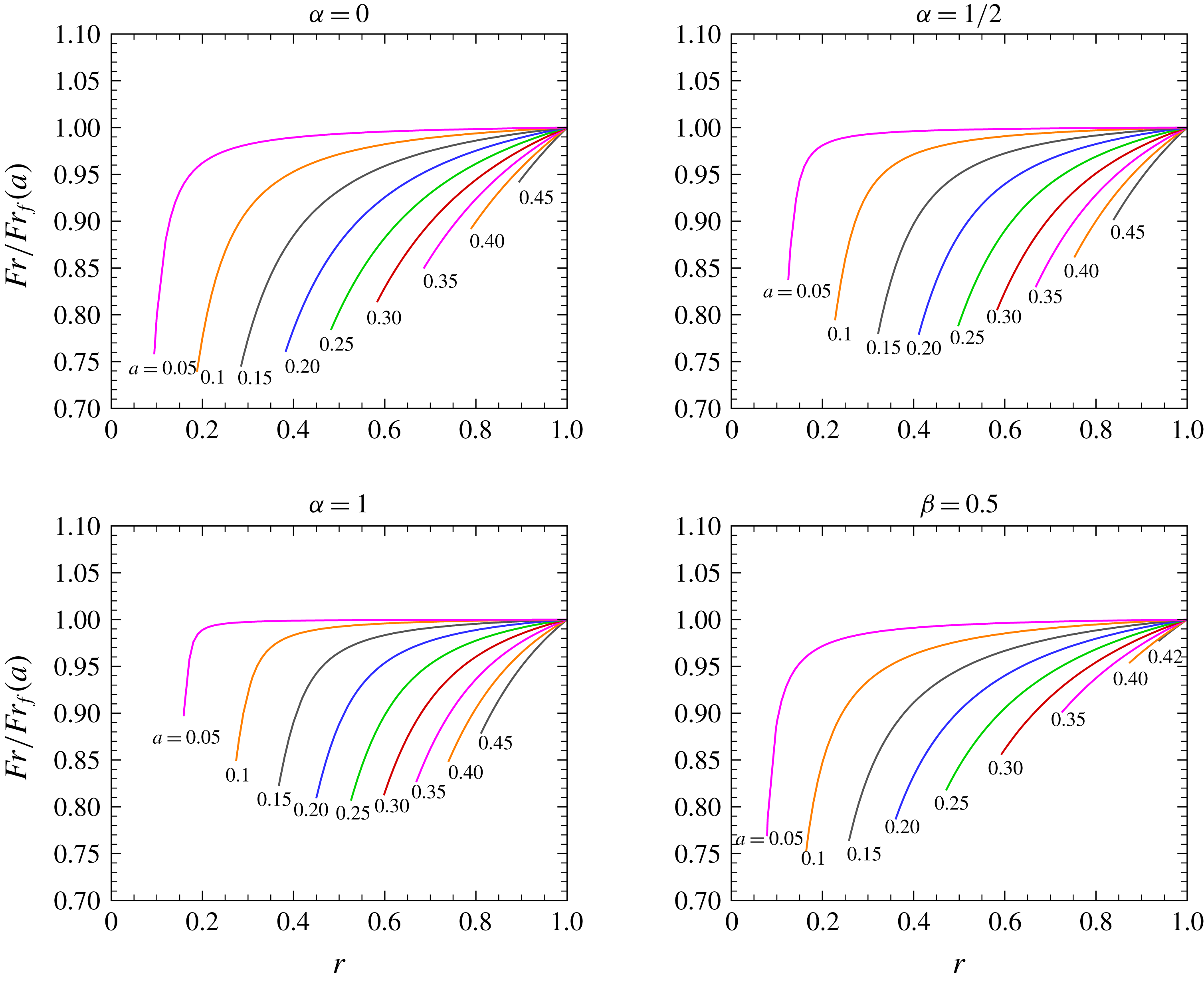
Figure 5 presents the results in the form of the ratio of the open-top
 $Fr(a,r)$
to the fixed-top
 $Fr_{f}(a)$
in the same
 $f(z)$
channel. We observe a consistent decrease of this ratio upon departure from the Boussinesq
 $r=1$
point, where
 $Fr(a,r)$
and
 $Fr_{f}(a)$
coincide. (Recall that
 $Fr_{f}(a)$
is shown in figure 2.)
Rate of dissipation
 $\dot{{\mathcal{D}}}/[\unicode[STIX]{x1D70C}_{2}(g^{\prime }h)^{3/2}A_{1}]$
versus
 $r$
for various
 $a$
, for triangle
 $\unicode[STIX]{x1D6FC}=1$
and trapezoid with
 $\unicode[STIX]{x1D6FD}=0.5$
.

Plots of
 $a_{max}$
,
 $a_{crit}$
,
 $\tilde{\unicode[STIX]{x1D712}}_{max}$
and energy-conserving
 $Fr(a_{max},r)$
scaled with
 $Fr_{f}(a_{max})$
versus
 $r$
, for triangle
 $\unicode[STIX]{x1D6FC}=1$
and trapezoid with
 $\unicode[STIX]{x1D6FD}=0.5$
.

Figures 6 and 7 compare salient results for the
 $\vee$
triangle (
 $\unicode[STIX]{x1D6FC}=1$
) to the trapezoid with
 $\unicode[STIX]{x1D6FD}=0.5$
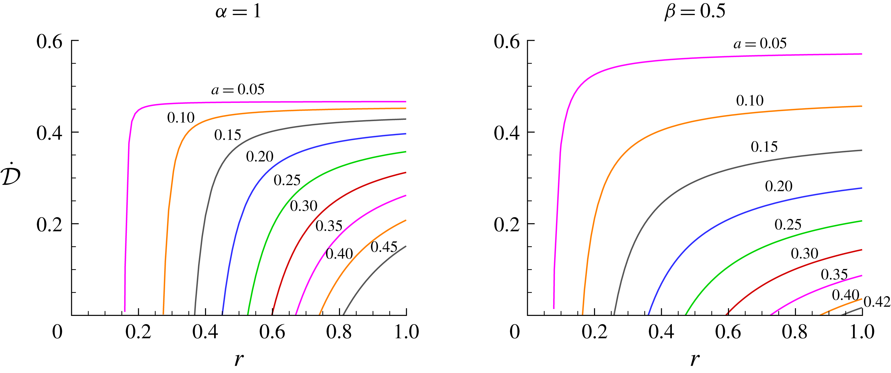
. The first comparison concerns the rate of dissipation, shown in figure 6 as a function of
 $r$
for fixed
 $a$
values. The qualitative behaviour is similar for triangle and trapezoid: for fixed
 $r$
, the scaled
 $\dot{{\mathcal{D}}}$
is larger for thin currents (small
 $a$
); for a fixed
 $a$
, the dissipation increases with
 $r$
. The dissipation in the contracting cross-section (trapezoid
 $\text{}\underline{/~\backslash }$
) is larger than in the expanding cross-section (
 $\vee$
triangle). Thin and less dense (larger
 $r$
) currents are more dissipative than the higher and more dense counterparts, but in general a significant dissipation accompanies the motion.
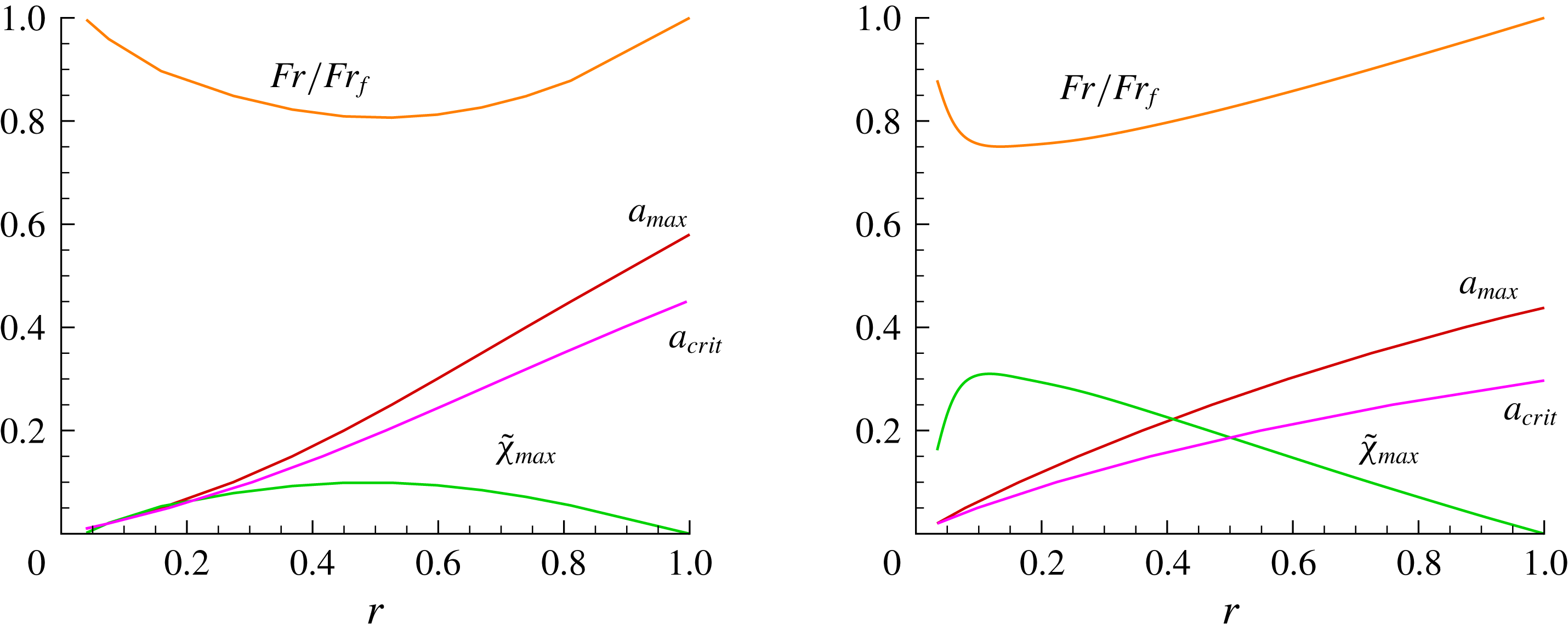
Figure 7 shows
 $a_{max}$
, the
 $h/H$
thickness of the energy-conserving current, which also gives the limit of energy validity (maximum thickness) as a function of
 $r$
. In general, the energy-validity criterion,
 $a_{max}$
, becomes more restrictive as
 $r$
decreases. The limit of sub-critical flow,
 $a_{crit}(r)$
, explained in appendix A, is also shown; this line is slightly below the
 $a_{max}(r)$
line. Our tests show that the difference of
 $Fra^{1/2}$
between the ‘max’ and ‘crit’ lines is small, which indicates that it is difficult to distinguish between energy-conserving and critical speed of propagation. The
 $\tilde{\unicode[STIX]{x1D712}}_{max}$
line shows the values of
 $\tilde{\unicode[STIX]{x1D712}}$
at the energy-conserving point, i.e. for
 $a=a_{max}$
, as a function of
 $r$
. Interestingly, our tests show that this is the maximum value of
 $\tilde{\unicode[STIX]{x1D712}}$
for a given
 $r$
. The
 $Fr$
ratio line shows, again, the values at the energy-conserving point, i.e. for
 $a=a_{max}$
, as a function of
 $r$
. Our tests show that this is the minimum value of
 $Fr/Fr_{f}$
for a given
 $r$
. We could not derive an analytical proof for the coincidence between
 $a_{max}$
,
 $\tilde{\unicode[STIX]{x1D712}}_{max}$
and minimum
 $Fr/Fr_{f}$
. The qualitative explanation is as follows. Consider the behaviour of
 $\tilde{\unicode[STIX]{x1D712}}=\unicode[STIX]{x1D716}\,a(1-Fr^{2}/2)$
, for fixed
 $\unicode[STIX]{x1D716}\,$
(and
 $r$
). Starting with some small
 $a$
where
 $Fr^{2}=2^{-}$
, we increase
 $a$
until
 $a=a_{max}$
. We know from various estimates and inspection of results that
 $Fr(a,r)$
is a decreasing function of
 $a$
. Since
 $Fr$
decreases,
 $a(1-Fr^{2}/2)$
increases continuously, and hence
 $\tilde{\unicode[STIX]{x1D712}}_{max}$
is attained at
 $a_{max}$
.
The remarkable difference in figure 7 is in the
 $\tilde{\unicode[STIX]{x1D712}}_{max}$
line: the values in the contracting
 $\text{}\underline{/~\backslash }$
geometry are significantly larger than in the expanding
 $\vee$
cross-section. Given the nonlinear nature of the balances, the interpretation is not clear. A tentative explanation is provided by the effect of the geometry on the behaviour of
 $Fr$
(see figure 2):
 $Fr^{2}/2$
is larger, closer to
 $1$
, in the triangle, and hence
 $\tilde{\unicode[STIX]{x1D712}}\propto (1-Fr^{2}/2)$
is smaller in the triangle than in the trapezoid.
To summarize, the shown results (figures 4–7) demonstrate that the present formulation yields physically acceptable results for
 $Fr$
and
 $\tilde{\unicode[STIX]{x1D712}}$
, for various
 $f(z)$
. The domain of validity is large. For a given cross-section geometry, the results are continuous functions of two parameters,
 $a$
and
 $r$
. The qualitative dependency on these parameters is the same for all the tested cases, but the geometry
 $f(z)$
affects significantly the quantitative details.
For a given
 $a$
, as
 $r$
decreases from 1,
 $Fr$
decreases (from the fixed-top value
 $Fr_{f}(a)$
),
 $\tilde{\unicode[STIX]{x1D712}}$
increases (from 0) and the dissipation decreases (from the fixed-top value). The maximum
 $\tilde{\unicode[STIX]{x1D712}}$
and reduction of
 $Fr$
are obtained at the energy-conserving point (the value of
 $r$
where
 $a$
intersects the
 $a_{max}(r)$
line). The dependency on
 $r$
is more pronounced for converging
 $f(z)$
(the trapezoid
 $\text{}\underline{/~\backslash }$
) than for diverging width (the
 $\vee$
triangle.)
We also obtained solutions (not shown here) for other cases, in particular power law with
 $\unicode[STIX]{x1D6FC}=1.5$
, expanding trapezoid
 $\backslash \text{}\underline{~}/$
with
 $\unicode[STIX]{x1D6FD}=-0.5$
and circle
 $f(z)=2(2Rz)^{1/2}(1-z/(2R))^{1/2}$
for various
 $R/H\geqslant 1/2$
. The solutions converged without difficulties, and the trends are consistent with the reported cases. In particular, we found that the agreement between the circle and the
 $bz^{1/2}$
approximation is good for
 $R/H>1$
, and improves as
 $R/H$
increases.
The uniqueness of the solution-by-iteration of a high-order nonlinear equation (or system) is a matter of concern in general. We addressed this issue by starting the iterations, for fixed
 $a$
and
 $r$
, at various points
 $Fr^{2}\in (0,2)$
. We found that when the iterations converged to a solution with positive
 $\unicode[STIX]{x1D712}$
, it was always the same result. We infer that there are no other solutions in the domain reported in the figures.
4 Concluding remarks
We have presented a comprehensive analysis of the idealized steady-state current of height
 $h$
and density
 $\unicode[STIX]{x1D70C}_{1}$
that propagates into an ambient unperturbed fluid of height
 $H$
and density
 $\unicode[STIX]{x1D70C}_{2}$
with an upper surface open to the atmosphere (open channel), at large
 $Re$
. We focused attention on channels of non-rectangular cross-section defined by a fairly general width function
 $f(z)$
. This is a significant generalization of Benjamin’s (Reference Benjamin1968) seminal analysis performed for a 2D (rectangular or laterally unbounded) cross-section with a fixed-top channel. Two previous extensions were available: the current in a general cross-section with a fixed top and the current in a 2D cross-section with an open top (Ungarish Reference Ungarish2012, Reference Ungarish2017). We demonstrate that in the general case a steady-state solution exists: the current propagates with
 $U$
and causes a depth decrease
 $\unicode[STIX]{x1D712}$
of the top surface.
The dimensionless parameters of the problem are
 $a=h/H$
and
 $r=\unicode[STIX]{x1D70C}_{2}/\unicode[STIX]{x1D70C}_{1}$
. The geometry enters the formulation via the width function
 $f(z),z\in [0,H]$
. We showed that a c.v. analysis produces a coupled set of equations for
 $\tilde{\unicode[STIX]{x1D712}}=\unicode[STIX]{x1D712}/H$
and
 $Fr=U/(g^{\prime }h)^{1/2}$
as functions of
 $a$
and
 $r$
. The balances are for volume and momentum. The formulation is self-contained without any adjustable constants. The currents are in general dissipative, and thus valid only for
 $a\leqslant a_{max}(r)$
. The current with height
 $h=a_{max}H$
is energy conserving. We demonstrated that in the Boussinesq limit
 $r\rightarrow 1$
, the open-top and fixed-top results coincide. The solution is not amenable to simple analytical presentation, but reliable and insightful results are easily obtained by numerical iterations. The criterion for critical propagation (with respect to the characteristics of the shallow-water equations),
 $a\leqslant a_{crit}$
, was also considered.
The significant difference with the fixed-top solution is the dependency of the
 $Fr$
,
 $a_{max}$
and
 $a_{crit}$
open-top results on two parameters:
 $a=h/H$
and
 $r=\unicode[STIX]{x1D70C}_{2}/\unicode[STIX]{x1D70C}_{1}$
. We reiterate that in the fixed-top case
 $Fr_{f}$
,
 $a_{max}$
and
 $a_{crit}$
are functions of
 $a$
only. (For given geometry
 $f(z)$
.)
The cross-section geometry influences quantitatively the results. We presented detailed solutions for a semi-circle,
 $\vee$
triangle and trapezoid (converging upward
 $\text{}\underline{/~\backslash }$
), and also for a rectangle for comparison. We found that
 $Fr(a,r)$
is typically smaller than the fixed-top
 $Fr_{f}(a)$
, but the reduction is not dramatic, typically a few per cent. For a given
 $r$
, the maximum height depression, and the minimum
 $Fr(a,r)/Fr_{f}(a)$
, are attained for the energy-conserving
 $a_{max}$
. The influence of the shape is more pronounced for a converging geometry (from bottom to top, like
 $\text{}\underline{/~\backslash }$
) than for a diverging one (like
 $\vee$
triangle).
Our model allows straightforward solution for other geometries. Interestingly, the sidewall contours
 $y=-f_{I},y=f_{II}$
enter the solution only in the combination
 $f(z)=f_{I}+f_{II}$
. This introduces useful similarities. For example: (i) triangles of different wedge angle share the same
 $Fr$
; (ii) channels with parallel sidewalls
 $f_{I}-f_{II}=\text{const}$
. can be treated as a rectangle; and (iii) a symmetric channel with
 $f_{I}=f_{II}$
is similar to the half
 $0\leqslant y\leqslant f_{II}$
. These features reflect the dominance of the inertia and pressure forces, which are not affected by the details of the bounding surface. These similarities should be carefully reconsidered when viscous friction becomes significant.
The presence of a fixed top was a major assumption in Benjamin’s (Reference Benjamin1968) seminal
 $Fr$
solution for a 2D current. We think that the relaxation of this quite strong restriction in the solution for a steady-state current in a general cross-section provides significant progress. The underlying ideas are the same: perform a c.v. steady-state analysis for the volume continuity and flow forces with free-slip boundary conditions, and subject to the presence of a non-negative energy dissipation (headloss) along the streamlines that cross the c.v. The current is motionless in the attached c.v. The upstream and downstream velocities are constant, and hence in these domains the pressure is hydrostatic. The pressure-loop continuity matches between the vertical-hydrostatic and horizontal-dynamic pressure differences. The prediction power of this model is remarkable. In a broad range of cases of interest, the ratio
 $U/(g^{\prime }h)^{1/2}$
, called
 $Fr$
, is of the order of unity, and can be calculated with simple analytical or semi-analytical methods. The range of validity, rate of energy dissipation and depression of the top open surface (when applicable) can also be calculated. The model is self-contained, with no adjustable constants. However, we keep in mind that the energy dissipation (headloss) in this model is distributed over all the downstream flux of the ambient, while physical considerations restrict these effects to a layer (wake) about the interface. The remedy of this deficiency requires a significant research effort, which is left for future work.
With hindsight, it is puzzling as to why Benjamin was so adamant about the need for a fixed top in the model for
 $Fr$
. We can speculate that Benjamin’s objective was a simple analytical formula for
 $Fr$
, which can be indeed obtained only for the fixed-top case. We can also suggest that Benjamin’s focus was on Boussinesq currents; in this case the fixed-top simpler model provides the needed
 $Fr$
with less effort.
The present results provide a unified/general theory for flow field and nose jump conditions prediction in channels of various cross-sections with a top boundary that is closed (fixed) or open to the atmosphere, for the full range of density ratio,
 $0<r=\unicode[STIX]{x1D70C}_{2}/\unicode[STIX]{x1D70C}_{1}<1$
. The previously investigated Benjamin-type steady-state
 $Fr$
and dissipation results are included:
 $f(z)=$
const. reproduces the 2D results, and
 $\unicode[STIX]{x1D712}=0$
recovers the fixed-top solution.
Admittedly, both the fixed- and open-top models are strong idealizations. The steady-state flow must be consistent with initial and boundary conditions, which is usually attainable when
 $U$
is sub-critical (or at most critical) with respect to the speed of the characteristic. This, however, turns out to produce only a mild additional restriction
 $a\leqslant a_{crit}$
, discussed in appendix A and displayed in figure 7. In a realistic flow the interface shear domain spreads (mildly) with
 $\sqrt{x}$
behind the c.v., as already pointed out by Benjamin. Moreover, the conditions of free-slip side, top and bottom boundaries can be realized in Navier–Stokes simulations, but in the laboratory and in nature some (small but finite) shear (and surface tension) is present. Still, the analysis is expected to provide the correct parametric insights, be a fair approximation for a limited period/distance of propagation of currents created by a constant source or lock release and be useful as a ‘jump condition’ at the nose of more complicated currents.
To our knowledge, no data for a reliable comparison with the present theory are available. The available open-channel laboratory studies for the considered problem are for Boussinesq liquids with
 $r\approx 1$
. In this case
 $\unicode[STIX]{x1D712}/H$
is small, and the difference between the open-surface and fixed-top predictions is in the range of the experimental error (a few per cent). Consider for example the available lock-release experiments for the
 $\vee$
triangle and semi-circle reported by Ungarish, Mériaux & Kurz-Besson (Reference Ungarish, Mériaux and Kurz-Besson2014) and Longo et al. (Reference Longo, Ungarish, Di Federico, Chiapponi and Maranzoni2015), respectively. The experimental tanks were open to the atmosphere, but the results were analysed by a fixed-top theory. The typical height
 $H$
was
 $6.7$
cm for the triangle and
 $9.5$
cm for the semi-circle. The fluids were saline and fresh water, and the largest density contrast
 $\unicode[STIX]{x1D716}\,$
was
 $0.11$
. Using fixed-top theory we find the thickness of the current at nose
 $h\approx 0.4$
cm, and
 $Fr_{f}\approx 1$
. This indicates the open-surface depression
 $\unicode[STIX]{x1D712}\lesssim 0.2$
cm (see (2.5)). It is difficult to measure accurately such small variations of the surface, and in any case these experiments were concerned with the current, not with data acquisition for
 $\unicode[STIX]{x1D712}$
. We can use the open-surface theory to evaluate
 $Fr/Fr_{f}=0.96$
for the triangle and
 $0.97$
for the semi-circle. This indicates a 3 %–4 % reduction of propagation speed
 $u_{N}$
as compared with the fixed-top prediction. The measured
 $u_{N}$
was smaller than the fixed-top predictions by 15 %–20 %, and hence, although the open-top theory improves the agreement by 3 %–4 %, a clear-cut quantitative conclusion is not possible. For sharper conclusions, tests with a larger density contrast, and with very accurate record of the shape of the open interface, are needed. Laboratory tests, and Navier–Stokes simulations, for non-Boussinesq currents with an open surface are difficult and expensive tasks (as compared to the fixed-top and Boussinesq counterpart), and the non-rectangular cross-section increases the challenge. We hope that this study will provide motivation and guidelines for such works in the future. An investigation for currents created by lock release in a channel with circular cross-section for
 $r\in (0.58,0.94)$
is underway (Longo et al.
Reference Longo, Ungarish, Chiapponi, Petrolo and Di Federico2018a
).
This study considers only flows with
 $Fr^{2}<2$
in which the current causes a depression (positive
 $\unicode[STIX]{x1D712}$
) of the free-top surface. Rapid currents with
 $Fr^{2}>2$
which elevate the surface (negative
 $\unicode[STIX]{x1D712}$
) are formally possible, and require a separate investigation which is left for future work.
Appendix. Critical
$U$
and the
$a\leqslant a_{crit}$
restriction


We considered a steady-state GC without specifying when and how it has been generated. The connection with the more realistic current produced by lock release or inflow involves the use of the shallow-water (SW) equation time-dependent formulation which accounts for initial conditions. The analysis of resulting flow indicates that the quasi-steady nose domain of the GC is governed by the characteristics of the SW hyperbolic system. Theory and experiments, see Baines (Reference Baines1995), Ungarish (Reference Ungarish2011), indicate that a typical steady-state current does not move faster than the characteristic
 $c_{+}$
(from the reservoir of dense fluid to the nose). This suggests that the
 $Fr$
and
 $\tilde{\unicode[STIX]{x1D712}}$
results developed in this paper are relevant only when the propagation is sub-critical (or at most critical) with
 $c_{+}\geqslant U$
. Here we attempt to quantify this restriction.
To determine the speed of the characteristics we must use the SW equations for a two-layer system in a channel of width
 $f(z)$
with an open surface. The thicknesses of the layers are
 $h_{1},h_{2}$
and the area-averaged velocities (in the laboratory frame) are
 $u_{1},u_{2}$
, functions of
 $x$
and
 $t$
. Denote
 $h_{1}+h_{2}={\hat{H}}$
. It is convenient to scale the variables using a typical length
 $h_{0}$
, speed
 $(g^{\prime }h_{0})^{1/2}$
and time
 $h_{0}/(g^{\prime }h_{0})^{1/2}$
, where, again,
 $g^{\prime }=\unicode[STIX]{x1D716}\,g$
,
 $\unicode[STIX]{x1D716}\,=\unicode[STIX]{x0394}\unicode[STIX]{x1D70C}/\unicode[STIX]{x1D70C}_{2}=1/r-1$
.
The details of the derivation of the equations of motion will be presented elsewhere (Longo et al. Reference Longo, Ungarish, Chiapponi, Petrolo and Di Federico2018a ). The system can be written as
 $$\begin{eqnarray}\left(\begin{array}{@{}c@{}}h_{1}\\ u_{1}\\ {\hat{H}}\\ u_{2}\end{array}\right)_{t}+\left(\begin{array}{@{}cccc@{}}u_{1} & \frac{\displaystyle A_{1}}{\displaystyle f(h_{1})} & 0 & 0\\ r & u_{1} & {\displaystyle \frac{r}{\unicode[STIX]{x1D716}\,}} & 0\\ (u_{1}-u_{2}){\displaystyle \frac{\displaystyle f(h_{1})}{\displaystyle f({\hat{H}})}} & \frac{\displaystyle A_{1}}{\displaystyle f({\hat{H}})} & u_{2} & \frac{\displaystyle A_{2}}{\displaystyle f({\hat{H}})}\\ 0 & 0 & {\displaystyle \frac{1}{\unicode[STIX]{x1D716}\,}} & u_{2}\end{array}\right)\left(\begin{array}{@{}c@{}}h_{1}\\ u_{1}\\ {\hat{H}}\\ u_{2}\end{array}\right)_{x}=0.\end{eqnarray}$$
The characteristics are the eigenvalues
 $\unicode[STIX]{x1D706}_{i}$
of the matrix of coefficients, given by an algebraic equation of the fourth order. In this equation we substitute the critical-speed request
 $\unicode[STIX]{x1D706}=u_{1}$
and obtain the condition
 $$\begin{eqnarray}(u_{2}-u_{1})^{2}=\left[\unicode[STIX]{x1D716}\,+\frac{f(h_{1})}{f({\hat{H}})}\right]^{-1}\frac{A_{2}}{f({\hat{H}})}.\end{eqnarray}$$
We apply this condition to the nose of the GC where
 $u_{1}=U=Frh^{1/2}$
,
 ${\hat{H}}=H(1-\tilde{\unicode[STIX]{x1D712}})$
,
 $h_{1}=h$
(of the current) and
 $|u_{2}-u_{1}|=(A_{0}/A_{2})U$
(see figure 3). We obtain
 $$\begin{eqnarray}Fr^{2}a=\frac{A_{2}^{3}}{A_{0}^{2}Hf(H-\unicode[STIX]{x1D712})}\left[\unicode[STIX]{x1D716}\,+\frac{f(h)}{f(H-\unicode[STIX]{x1D712})}\right]^{-1}.\end{eqnarray}$$
The solution determines the value of
 $a_{crit}$
. We argue that a current with a smaller
 $a$
propagates more slowly and hence the sub-to-critical domain is
 $a\leqslant a_{crit}$
. Numerical evaluation is needed because the right-hand side of (A 3) is in general a cumbersome expression of
 $a$
and
 $\tilde{\unicode[STIX]{x1D712}}$
. Even for the power-law
 $f(z)=bz^{\unicode[STIX]{x1D6FC}}$
the right-hand side is not insightful analytically. For the rectangular
 $f(z)=$
const. (A 3) can be reduced to
 $$\begin{eqnarray}Fr^{2}a=\frac{(1-a-\tilde{\unicode[STIX]{x1D712}})^{3}}{\unicode[STIX]{x1D716}\,+1},\end{eqnarray}$$
which indicates that the restriction becomes more severe as
 $\unicode[STIX]{x1D716}\,$
increases.
We remark that the present estimate is a tentative result. A more reliable critical-flow criterion requires the analysis of the dam-break Riemann problem of the (A 1) system, which is beyond the scope of the present work.
For the Boussinesq
 $\unicode[STIX]{x1D716}\,\rightarrow 0$
, (A 3) yields
 $$\begin{eqnarray}Fr^{2}a=(1-\unicode[STIX]{x1D711})^{3}\frac{A_{0}}{Hf(h)},\end{eqnarray}$$
where
 $\unicode[STIX]{x1D711}=A_{1}/A_{0}$
. This coincides with the fixed-top value (Ungarish Reference Ungarish2013).