


1. Introduction
Income-based consumption patterns play a critical role in determining CO2 emissions as they shape the demand for goods and services and the corresponding energy consumption (York et al., Reference York, Rosa and Dietz2003). The level of emissions depends on population growth, technological advancements, international trade and policy interventions (Grunewald and Martinez-zarzoso, Reference Grunewald and Martinez-Zarzoso2016). Research has shown that, as income rises, consumption patterns increase the energy intensity of goods and services such as larger homes, vehicles or increased travel (York et al., Reference York, Rosa and Dietz2003). Additionally, higher income levels often result in greater demand for imported goods that can indirectly contribute to supply chain CO2 emissions (Peters et al., Reference Peters, Minx, Weber and Edenhofer2011).
Chen et al. (Reference Chen, Duo, Zhao, Zeng and Guo2023) found that human activities are a major source of ecosystem vulnerability, and reducing emissions is the principal way to reduce vulnerability. Climate change adaptability invites countries to exhibit a greater inclination to undertake adaptation measures by capitalizing on public and private investments (Tol, Reference Tol2005). This is accomplished through governmental initiatives, raising community consciousness and enabling private sector engagement. Therefore, understanding the role of income-based consumption patterns in shaping CO2 emissions (as discussed by Kalim et al., Reference Kalim, Ul-Durar, Iqbal, Arshed and Shahbaz2024) is crucial for developing effective strategies to mitigate climate change. By examining the factors that drive environmental impacts, policymakers and researchers can better understand how to design and implement measures that encourage sustainable consumption and production patterns.
Historically, environmental deterioration has been positively correlated with economic performance. The environmental Kuznets curve (EKC) shows that there has been a different relationship between environmental quality and economic growth, particularly over the last two decades. The EKC hypothesis supports an inverted U-shaped environment and economic growth relationship (Disli et al., Reference Disli, Ng and Askari2016). As expansion accelerates in the early stages of development, greenhouse gases also rise, which ultimately leads to global warming and climate adaptability. Further developments in a country lead to a reduction in global warming due to improved attitudes of people towards resilience, forming a U-shaped climate adaptability – demand Kuznets curve. This can be explained through the development in human capital, as it is an increase in education and standard of living and so forth, which, in turn, leads to an improved level of understanding and awareness of the overall approach of citizens regarding environmental change, posterity and resilience and incorporates behaviour towards efficient and greener energy consumption (Lee et al., Reference Lee, Park, Lee, Park, Jeong and Kim2015).
The literature has also discussed the U-shaped effect of the load capacity curve (LCC) (Pata and Kartal, Reference Pata and Kartal2023), which indicates that an increase in income places a load on production systems beyond their capacity to manage, thereby leading to emissions, footprints and global warming (Iqbal et al., Reference Iqbal, Ul Durar, Arshed, Shahzad and Ayub2025). This phenomenon will explain the inverted U-shaped climate adaptability – demand LCC.
In the literature, many studies have shown concerns with challenges related to cultural and social aspects that are important to investigate one step beyond sustainable development (Bhattacharya et al., Reference Bhattacharya, Bhattacharya, Mclellan and Tezuka2020). Researchers like Adger et al. (Reference Adger, Barnett, Brown, Marshall and O'Brien2013) have given less attention to the role of cultural and social adaptation towards climate change and have instead discussed the capacity to mitigate climate adaptability; there is still a debate about what countries should do to abate climate change (Millner and Dietz, Reference Millner and Dietz2015). National culture as an informal institution is formed by interpersonal interactions and is ingrained in fundamental assumptions, values, beliefs and customs (Hofstede, Reference Hofstede2001). Individuals’ preferences and consumption habits vary as culture changes. This transition results from regional knowledge spillovers, technical advancements and institutional growth. These changes impact people’s purchasing habits by changing routines through employing cutting-edge, eco-friendly technology. Liu et al. (Reference Liu, Ciais, Deng, Lei, Davis, Feng, Zheng, Cui, Zhu, Guo, Ke, Sun, Han, Xue, Boucher, Boucher, Chevallier, Tanaka, Wei, Zhong, Kang, Zhang, Chen, Xi, Liu, Breon, Lu, Zhang, Guan, Gong, Kammen, He and Schellnhuber2020) verified that the decline of CO2 emissions varies between regions, countries and cultures. When people engage in a cultural dimension, such as long-term orientation, low uncertainty avoidance (UA), masculinity, indulgent societies, collectivism and low power distance, they tend to have a carbon literacy orientation (Arshed et al., Reference Arshed, Hameed, Saher and Yazdani2022). Since national culture establishes barriers to behaviour, it should impact an individual's ethical and responsible behaviour (Parboteeah et al., Reference Parboteeah, Bronson and Cullen2005). The different beliefs, values, attitudes, ideas and morals embedded in national culture guide individuals regarding acceptable and unacceptable behaviours (Vitell et al., Reference Vitell, Paolillo and Thomas2003).
Culture is reflected in society at various levels such as production and consumption processes, people’s lifestyles and institutional policies and actions that determine the level of carbon emission in society (Cronk, Reference Cronk1995). Culture plays a central role in determining the level of adaptability of all related actions in a society in the form of risk identification and taking measures to respond to environmental changes. Therefore, culture is placed in a central position that triggers changes in human lifestyle, consumption patterns, behaviour and responses. There is a lack of theoretical and empirical research addressing the need for adaptability required for social and cultural networks to determine the magnitude of necessary efforts to respond to carbon footprints (Mendonça et al., Reference Mendonça, De Andrade Conradi Barni, Moro, Bornia, Kupek and Fernandes2020).
This study examines the quadratic relationship between demand-led economic activity and climatic adaptability, taking into account the influence of contextualized national culture, in line with the findings of Arshed et al. (Reference Arshed, Hameed, Saher and Yazdani2022). Several prior research studies have examined the correlation between consumption patterns and CO2 emissions, as evidenced by the works of Saleem and Ali (Reference Saleem and Ali2019) and Shi et al. (Reference Shi, Li, Zhang, Liu, Li and Zhong2020). This research employs the EKC and LCC framework to analyse sustainable consumption patterns and examines the evolution of demand-driven behaviour in response to different cultural environments. Hence, the present study aims to examine the correlation between income and climate adaptability whilst considering cultural variations to emphasize the importance of sustainable cultural practices. The analysis extends the demand-led relationship in multiple ways. Firstly, it includes the environmental burden of development, captured using carbon emissions, and secondly, it applies dynamic panel data to control for persistence in adaptability, culture and demand. This study demonstrates that societies characterized by higher standards of living exhibit a greater capacity to adjust to environmental changes and offers a comprehensive analysis of policy tools to effectively mitigate climate risk.
2. Literature review and hypotheses development
The impacts of greenhouse gases on the atmosphere are becoming more pronounced daily (Houghton et al., Reference Houghton, Jenkins and Ephraums1990), which is endangering the global climate. Human activities are increasing these emissions that cause climate change and vulnerability. These human activities include population growth, technology, economic activities, political and economic institutions and human attitudes and beliefs (Wei et al., Reference Wei, Liu, Fan and Wu2007). Druckman and Jackson (Reference Druckman and Jackson2008) examined how income and socioeconomic characteristics influence household energy consumption in the United Kingdom and found that wealthier households often use more energy, leading to an increase in carbon emissions. Reinders et al. (Reference Reinders, Vringer and Blok2003) explored the impact of household spending and CO2 in 11 European Union nations, explaining indirect energy demand. Ivanova et al. (Reference Ivanova, Standler, Steen-Olsen, Wood, Vita, Tukker and Hertwich2016) examined how household consumption affects the environment and found that higher-income households have a larger environmental footprint since they consume more products and services. Therefore, high-income lifestyles must be markedly adjusted to maintain sustainability and lessen climate adaptability and readiness (O'neill et al., Reference O'neill, Fanning, Lamb and Steinberger2018). Lenzen et al. (Reference Lenzen, Moran, Kanemoto, Foran, Lobefaro and Geschke2012) studied global sustainable household energy consumption. They demonstrated that the Kuznets curve is unsupported and that energy requirements vary among cultures and nations. Kalim et al. (Reference Kalim, Ul-Durar, Iqbal, Arshed and Shahbaz2024) indicated that the sustainable portion of the EKC is only feasible when appropriate intervention introduces sustainable practices, which guides this study to use moderating effects.
Wei et al. (Reference Wei, Liu, Fan and Wu2007) explored the lifestyle implications in urban and rural families in China between 1999 and 2002. The researchers investigated the direct and indirect effects of these lifestyle factors on energy consumption and carbon dioxide emissions. Schipper et al. (Reference Schipper, Bartlett, Hawk and Vine1989) identified a significant portion, ranging from 45 to 55 per cent, of the overall energy that is consumed by consumer-related activities, including but not limited to housing, travel and various services. Hence, the utilization of technology and the lifestyle choices of individuals significantly determine energy consumption and subsequent CO2 emissions. The concept of lifestyle was initially established in a study conducted during the late 1980s (Schipper et al., Reference Schipper, Bartlett, Hawk and Vine1989), which specifically examined the impact of consumer behaviour on energy use. Bin and Dowlatabadi (Reference Bin and Dowlatabadi2005) introduced a consumer lifestyle framework to examine the impact of demander actions on environmental outcomes inside the United States of America (USA). Consumer demands and the corresponding economic activities in the USA contribute to about 80 per cent of the total energy consumption and carbon dioxide emissions. Consumer-related activities, including personal travel and residential energy usage, are a notable portion of the USA’s gross domestic product, amounting to 4 per cent. However, these activities have a significantly larger impact on both energy consumption and CO2 emissions, accounting for 28 and 41 per cent, respectively.
Lifestyle is different ways of existence that individuals and organizations accomplish through accepted socially and culturally comprehensible patterns of behaviour (Lutzenhiser and Gossard, Reference Lutzenhiser and Gossard2000). Households consume more energy with the progress in globalization, population and culture. Adapting to the way of life and culture of rich nations, households in emerging nations are using more energy to maintain their standard of living (Gupta, Reference Gupta2011). Furthermore, consumption patterns may change to favour more energy-intensive goods and services as income levels grow; for instance, people might buy bigger homes or cars, go on more trips or buy more electronics and equipment. Studies like Arshed et al. (Reference Arshed, Hameed, Saher and Yazdani2022) and Kalim et al. (Reference Kalim, Ul-Durar, Iqbal, Arshed and Shahbaz2024) have confirmed similar outcomes relating consumption patterns to CO2 emissions.
Researchers and decision-makers now intend to explore climate change issues caused by anthropogenic (human) activities. Global warming is a concern that has a distributional effect on all countries (Mendelsohn et al., Reference Mendelsohn, Dinar and Williams2006). According to the Intergovernmental Panel on Climate Change (IPCC), greenhouse gas emissions, of which carbon emissions account for 73 per cent, are to blame for the approximately 0.6°C warming of Earth’s surface over the twentieth century (Zhang et al., Reference Zhang, Liu and Bae2017). Anthropogenic activities are changing this cycle by increasing the level of atmospheric carbon emissions or what is known as the ecological footprint (Disli et al., Reference Disli, Ng and Askari2016). According to IPCC estimates, compared to the pre-industrial era (1750–1900), anthropogenic activities boosted global warming by around 1°C. Between 2030 and 2052, global temperature is expected to increase by approximately 1.5°C if current trends continue (IPCC, 2018).
According to research by Poumanyvong et al. (Reference Poumanyvong, Kaneko and Dhakal2012), urbanization and development lead to higher transportation energy consumption, which is more pronounced in nations with higher income levels. According to the research by Al-mulali et al. (Reference Al-Mulali, Binti Che Sab and Fereidouni2012), there is a high development, energy demand and CO2 emissions correlation in 80 per cent of the nations, with the degree of development in each country affecting this link. O'neill et al. (Reference O'neill, Fanning, Lamb and Steinberger2018) state that China’s faster economic progress and labour supply impact energy use and CO2 emissions. Zhu et al. (Reference Zhu, You and Zeng2012) examined 20 emerging nations and discovered that urbanization, development and CO2 emissions correlate in an inverted U pattern.
Increased income-based consumption can lead to overexploiting natural resources, such as water, land and forests, for agricultural, industrial and urban development purposes. This overconsumption can exacerbate environmental degradation and contribute to climate change by altering ecosystems and releasing more greenhouse gases into the atmosphere (Jorgenson and Clark, Reference Jorgenson and Clark2012). O'neill et al. (Reference O'neill, Fanning, Lamb and Steinberger2018) argue that rising income levels, particularly in developing countries, could lead to increased consumption and, consequently, increased greenhouse gas emissions, thus contributing to climate change. High-income individuals are responsible for a disproportionately large share of carbon emissions (Chancel and Piketty, Reference Chancel and Piketty2015).
Income-based consumption can lead to disparities in climate adaptability between different income groups and regions. For instance, wealthier individuals and countries have more resources to invest in adaptation and resilience measures to cope with climate change impacts. At the same time, poorer populations are often more vulnerable due to their limited resources and adaptation capacity (Adger et al., Reference Adger, Barnett, Brown, Marshall and O'Brien2013). Grubler et al. (Reference Grubler, Wilson and Nemet2016) examine the role of technological innovation in shaping energy transitions. As economies develop, technological advances can facilitate the shift towards cleaner, more efficient energy sources and reduce the negative impacts of income-based consumption on climate adaptability. While economic development can lead to increased consumption and climate vulnerability, over time – as economies develop – advances in technology, education and awareness can help counteract these negative effects. Development can reduce climate vulnerability by fostering cleaner technologies, informed consumption decisions and sustainable practices and thus promote a more sustainable future (Kusumawardani and Dewi, Reference Kusumawardani and Dewi2020). This shows that income-based consumption and climate adaptability form non-linear relationships depending on time and development in a country.
However, the EKC in particular has demonstrated a divergent link between economic progress and the environment over the last two decades. Economic success has a positive historical correlation with environmental deterioration. The EKC shows a relationship between economic progress and environmental pollution that is an inverted U-shape (Disli et al., Reference Disli, Ng and Askari2016). According to this, the early phases of development see increased expansion, which causes greenhouse gas levels to rise and, ultimately, causes global warming, climate change and adaptability. As consumers become more aware of environmental issues, greenhouse gas emissions decline (Dinda, Reference Dinda2004). The effectiveness of adaptability depends on economic, governmental and social readiness. Economic readiness is the investment climate that permits private sector capital mobilization. Therefore, H1 is as follows.
H1: Income-based consumption forms an EKC relationship with climate adaptability.
Cultural values are established, and changes take place gradually; the influence of energy use on climate change may be lessened or enhanced due to different cultural elements heterogeneously. They influence how people behave in groups and as individuals when dealing with authority, self-concept and conflicts (Inkeles, Reference Inkeles2017). Consequently, cultural attitudes might positively or negatively impact energy consumption and CO2 emissions. Cultural values influence how organizations and people behave in relation to issues of authority, self-perception and other conflicts, as well as how they resolve these issues and difficulties (Inkeles, Reference Inkeles2017). For instance, Panayotou (Reference Panayotou1997) states that institutional variables, such as applying laws and contracts and securing property rights across all nations, can smooth out the EKC for CO2 emissions.
The capacity of society and its associated sectors to adapt helps mitigate possible harm and effectively address the adverse impacts of climatic disasters. One of the primary obstacles developing nations face is environmental concerns in the initial stages of their economic progress (Disli et al., Reference Disli, Ng and Askari2016). The onset of economic development was concomitant with the occurrence of pollution due to the prevailing emphasis on economic growth in many societies, which led to a disregard for environmental considerations such as the maintenance of clean air, water and land utilization (Dasgupta et al., Reference Dasgupta, Laplante, Wang and Wheeler2002). Individuals exhibit a greater concern for basic needs fulfilment through acquiring and consuming affordable goods, sometimes overlooking the ecological ramifications of such economic expansion. As individuals experience the fulfilment of their basic requirements and witness an increase in their income as a result of economic and institutional advancements, their appreciation for the environment becomes heightened. The individuals in question are preoccupied with using ecologically sustainable products that result in reduced emissions (Kohler, Reference Kohler2013).
National culture is shaping individuals’ and groups’ collaborations and interactions. These cultural dimensions contribute to the Kuznets curve between income-based energy consumption and climate adaptability separately.
2.1. High vs low power distance culture
According to Hofstede (Reference Hofstede2001) and Kirkman et al. (Reference Kirkman, Lowe and Gibson2006), power distance measures how unequally a country’s or an organization’s members are distributed in terms of power and how much they accept this unequal distribution. Higher power distance nations have explicit laws and regulations, authority concentration and undemocratic decision-making processes.
Instead of considering the benefits and interests of the general public, decisions are predominantly based on favouritism and loyalty in nations with a significant power distance (Hofstede, Reference Hofstede2001). High power distance nations surrender their ethical values for convenience and accessibility (Husted, Reference Husted2005). Metz (Reference Metz1991) discussed Nepal’s forestry program and claimed that increased power distance could hinder the effectiveness of the program because bureaucrats implement programs with a greater emphasis on sponsors compared to technical proficiency.
In high power distance societies, decision-making and resource allocation are often centralized with power concentrated among a few individuals or groups. This may lead to a focus on projects and investments that benefit these powerful entities rather than a broader, more equitable distribution of resources. In contrast, low power distance societies tend to have more inclusive decision-making processes, which could lead to a more equitable distribution of resources and investments that promote energy efficiency and renewable energy.
Based on the literature, it is contended that hierarchical systems are used in high power distance nations, with decisions being taken at the top. On the one hand, high power distance prevents subordinates from contributing, while, on the other hand, alienating them from the nation’s overall industrial processes (Hofstede, Reference Hofstede1999). High power distance societies may be more resistant to implementing strict environmental policies as influential individuals or groups could perceive these policies as threats to their interests or status. High power distance societies may enforce environmental regulations less effectively as lower-ranking individuals may hesitate to challenge authority or report violations. Businesses in such countries prioritize profits over environmental performance or product quality, and they ignore consumer behaviour because they do not ask for input from the public. The following hypothesis was developed based on the above discussion.
H2: High power distance shifts the EKC of income-based consumption and climate adaptability upward.
2.2. Individualism vs collectivism culture
Individualism and collectivism are two distinct cultural dimensions that describe how people prioritize their or the group’s interests. Understanding individualism and collectivism can help provide insights into how cultural values shape human behaviour, decision-making and social norms across different societies (Hofstede, Reference Hofstede1999).
Individualism characterizes societies where individuals prioritize their own needs, desires and interests and those of their immediate family members. Individualistic cultures highly value personal autonomy, individual rights and self-expression (Traintis, Reference Traintis2002). Individualism represents a society in which there are few relationships between people, and everyone is expected to take care of themselves and their immediate family (Hofstede et al., Reference Hofstede, Hofstede and Minkov2010). Rawwas et al. (Reference Rawwas, Swaidan and Oyman2005) stated that individualistic cultures have the propensity to prioritize individual objectives and passions over shared interests. Hence, when individuality rises, individuals are more likely to accept unethical behaviours. In contrast, people in a collectivist culture protect the interests of their group. In collectivist cultures, people often have strong, cohesive in-group relationships and feel a strong sense of responsibility to support and contribute to the group’s well-being (Hofstede, Reference Hofstede2001). Loyalty, harmony and conformity are highly valued in these societies (Gudykunst et al., Reference Gudykunst, Matsumoto, Ting-Toomey, Nishida, Kim and Heyman1996). Collectivists’ actions are intended to advantage their in-group even if the individual themselves suffers.
Individualism versus collectivism illustrates the type of relationship between individuals and the groups to which they belong (Hofstede, Reference Hofstede2001). Due to the dominance of the independent ego and self-preference, Komatsu et al. (Reference Komatsu, Rappleye and Silova2019) discovered that individuals in individualistic societies are less likely to assume that human activities contribute to environmental problems (i.e., lower levels of anthropogenic perception). Due to these low levels of anthropogenic perception, people in individualistic societies are less likely to consciously plan pro-environmental action, which, therefore, has a greater negative impact on the environment. Even among nations with comparable levels of anthropogenic perception, those with individualistic societies would have worse environmental effects because they would have less self-control when compelled to choose between their own interests and the interests of in-groups. People in collectivist societies are more likely to prioritize environmental integrity and sustainability, with readiness to adapt to those environmental changes because, according to Welsch (Reference Welsch2006), these factors contribute to the well-being of the group. Thus, this study develops the following hypothesis.
H3: High collectivism shifts the EKC of income-based consumption and climate adaptability downward.
2.3. High vs low UA culture
UA implies the degree to which vague and unknown situations are endangering to individuals, the extent to which orders and rules are favoured and the extent to which individuals in a society accept uncertainty (House et al., Reference House, Hanges, Javidan, Dorfman and Gupta2004). High UA cultures frequently rely on laws, regulations, norms, values and conventions to eliminate uncertainty in the face of ambiguous circumstances. Comparatively, weak UA cultures are more inclined to exhibit and accept deviation from accepted standards, norms and values of behaviour (Hofstede, Reference Hofstede1999, Reference Hofstede2001).
Parboteeah et al. (Reference Parboteeah, Bronson and Cullen2005) argue that individuals seek to avoid uncertainty and confusing situations in high UA societies. When avoiding uncertainty is the first choice of individuals in a situation, organizations, individuals and groups in such a society often adopt norms, values and rules to manage uncertainty. Therefore, higher levels of UA culture societies develop the basic rules, policies and structures to address ambiguous and unknown environmental issues. Environmental changes are tough due to global warming and higher UA societies are highly aggressive in enhancing environmental performance (Disli et al., Reference Disli, Ng and Askari2016).
This study contends that people are more aware of their energy consumption in societies with higher levels of UA because they do not want to risk degrading the environment. Therefore, the purchasing patterns of individuals are adjusted to ensure that they do not skimp on quality goods. As a result, businesses in these nations or civilizations create high-quality goods and design production processes that do not harm the environment or generate emissions. Therefore, this study developed the following hypothesis.
H4: High UA shifts the EKC of income-based consumption and climate adaptability downward.
2.4. Masculinity vs femininity culture
Individuals in feminine societies are more likely to place high importance on their quality of life and helping others than on the benefits they receive from their jobs (Hofstede, Reference Hofstede2001), compared to money-oriented growth, economic development and wealth generation in masculine societies. The attention of feminist civilizations is social well-being and a clean environment (Eisler, Reference Eisler2010). In masculine cultures that prioritize economic growth, organizations focus on creating and manufacturing commodities without regard for environmental quality (Hofstede, Reference Hofstede1999). Individuals’ consumption behaviour and patterns in these societies stick to energy-intensive means to advance personal development and growth without regard for environmental protection.
H5: High masculinity shifts the EKC of income-based consumption and climate adaptability upward.
2.5. Long-term vs short-term orientation culture
The level of long-term thinking among a society’s members is known as long-term orientation. Long-term-oriented societies are more involved in economic development and ecological quality, while short-term-oriented societies emphasize their societal traditions (Hofstede, Reference Hofstede2001). Long-term-oriented cultures forego their present advantages in favour of their distant future goals (Laibson, Reference Laibson1997).
The short- and long-term orientations of the culture have an impact on society’s spending patterns as well; people use more energy, just as in cultures that prioritize the short term, at the expense of the environment's quality, whereas societies with a long-term perspective consider the environment’s quality and future needs while consuming energy and other resources. Thus, this study developed the following hypothesis.
H6: High long-term orientation shifts the EKC of income-based consumption and climate adaptability ability downward.
2.6. Indulgence vs restraint culture
Indulgence societies provide individuals with the unrestricted enjoyment of their natural existence while cultures with a more constrained cultural orientation impose regulations on the pursuit of personal fulfilment, thus exerting control over people’s natural inclinations for the purpose of maximizing societal benefits (Hofstede et al., Reference Hofstede, Hofstede and Minkov2010). Cultures characterized by restraint exert influence over individuals’ lifestyles while societies that lean towards indulgence prioritize the pursuit of pleasure and the use of financial resources. This propensity for indulgence fosters a culture that encourages pollution and disregards sustainable practices. In contrast, restraint societies prioritize the establishment of norms, values, regulations and controlled behaviours that effectively mitigate pollution levels (Disli et al., Reference Disli, Ng and Askari2016).
Societies with restrained and regulated behaviours typically have more tightly controlled consumption patterns that allow for responsible energy use. People are permitted to use resources freely in indulgence societies to satisfy their wishes and enjoy their lives. Therefore, the following hypothesis was developed.
H7: High indulgence shifts the EKC of income-based consumption and climate adaptability upward.
3. Methodology
3.1. Variables and data sources
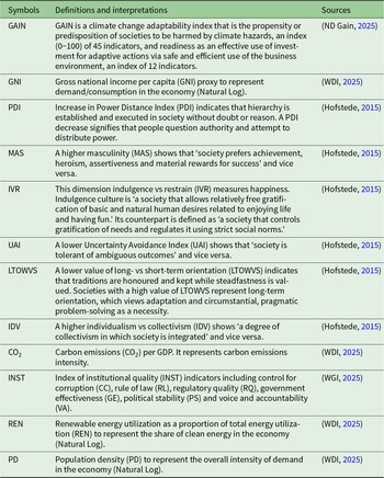
Table 1 reports the list of variables selected for the empirical investigation of the study framework. The sources of data are also provided. The dataset comprises 53 countries (see Supplementary Appendix Table A1) from 1998 to 2024. In contrast, six time-invariant culture indicators (IDV, PDI, UAI, LTOWVS, MAS and IVR, defined in Table 1) were collected from Hofstede’s cultural dimensions and used to moderate the GNI–GAIN relation. The dependent variable is GAIN, which is an index of climate change vulnerability and economic readiness; this study suggests it as climate adaptability.
Construction of variables and data sources

Table 1 Long description
Variable definitions and data sources for a study dataset covering climate adaptation, economic demand, cultural dimensions, emissions intensity, institutional quality, energy mix, and population pressure. GAIN is a climate change adaptability index combining vulnerability and readiness, scaled from 0 to 100 and built from multiple indicators. Economic demand proxies include gross national income per capita, renewable energy share, and population density, each specified as natural log transformed. Cultural measures come from Hofstede: power distance, masculinity, indulgence versus restraint, uncertainty avoidance, long-term versus short-term orientation, and individualism versus collectivism, with brief interpretations of what higher or lower values imply. Environmental pressure is represented by carbon emissions per unit of gross domestic product, described as emissions intensity. Institutional quality is a composite index drawing on governance dimensions such as corruption control, rule of law, regulatory quality, government effectiveness, political stability, and voice and accountability. Sources are ND Gain for GAIN, World Development Indicators for income, emissions, renewables, and population density, Worldwide Governance Indicators for institutions, and Hofstede for cultural indices. Interpretations describe directionality for several indices, but the table does not provide country values or time trends, only variable construction and provenance.
Source: Authors’ construction.
Gross national income (GNI) is used as an assessment of income-based consumption capacity, as it is a wider proxy of purchasing power. GNI captures broader coverage of permanent income capacity that shapes consumption, energy demand, lifestyle and adaptation investments compared to consumption expenditures. This study estimated institutional quality (INST) using principal factor analysis (Jackson, Reference Jackson2005) of six Worldwide Governance Indicators (WGI). This method reduces the dimensions from six to one while keeping the information intact and making the estimation model simpler and free of any possible collinearity. The quality of the index is assessed using eigenvalues and Kaiser–Meyer–Olkin (KMO) statistics.
3.2. Theoretical framework
Following the EKC of demand, the key idea is that consumers fulfil their needs at low income with minimal precedence for the sustainability and posterity of production procedures through which the merchandise is distributed. Thus, market influences do not induce sellers to choose sustainable and ecological production methods, thereby leading to a fall in adaptability 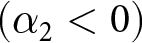 $({\alpha _2} \lt 0)$. At higher levels of demand, consumers buy higher-order products of Maslow’s hierarchy of needs theory to advantage themselves from luxury products which are ecologically vulnerable (Arshed et al., Reference Arshed, Munir and Iqbal2021). Beyond fulfilling basic needs, society allocates its income to environmentally responsible goods such that consumer forces compel producers to adopt cleaner production methods
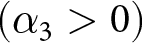 $({\alpha _3} \gt 0)$, increasing their resilience and adaptability. According to this study’s hypotheses, the national culture of the nation may be able to control the U-shaped EKC relationship’s turning point. As was noted in the literature, each factor of the national culture has a unique role in explaining the behaviour of consumers and buyers when their wages rise. Cultures such as risk-taking, masculinity and long-term orientation distinguish the purchasing patterns of consumers in a manner distinct from that of conventional EKC-based studies. This model is evaluated utilizing Equation (1).
Additional instruments for national culture are added to form six equations. Here, indicators of culture are multiplied by GNI and GNI2, wherein the first cross-product explains how culture alters the climate and negatively impacts consumption patterns  $({\alpha _5})$, and the second cross-product depicts how culture alters climate-resilient consumption patterns
 $({\alpha _6})$.
 \begin{align}{\text{GAI}}{{\text{N}}_{{\text{it}}}} &= {\alpha _1} + {\alpha _2}{\text{GN}}{{\text{I}}_{{\text{it}}}} + {\alpha _3}{\text{GNI}}_{{\text{it}}}^2 + {\alpha _4}{\text{CUL}} \times {\text{GN}}{{\text{I}}_{{\text{it}}}} + {\alpha _5}{\text{CUL}} \times {\text{GNI}}_{{\text{it}}}^2 + {\alpha _6}{\text{P}}{{\text{D}}_{{\text{it}}}} \nonumber\\
& \qquad\quad+ {\alpha _7}{\text{INS}}{{\text{T}}_{{\text{it}}}} + {\alpha _8}{\text{RE}}{{\text{N}}_{{\text{it}}}} + {\alpha _9}{\text{C}}{{\text{O}}_{{{\text{2}}_{{\text{it}}}}}} + {\varepsilon _{{\text{it}}}}.\end{align}
In Equation (1),  ${\text{GAI}}{{\text{N}}_{{\text{it}}}}$ is adaptability as an inverse measure of climate vulnerability of the possibility or propensity for climate risks to hurt human societies, as mentioned in Table 1. This is acquired from an open-source database called the Notre Dame-Global Adaptation Initiative (ND-GAIN) Country Index. Over 74 variables are combined by ND-GAIN to create 45 core indicators.
 ${\text{GN}}{{\text{I}}_{{\text{it}}}}$ is the log of GNI;
 ${\text{GNI}}_{{\text{it}}}^{\text{2}}$ is the log of GNI squared;
 ${\text{CU}}{{\text{L}}_{{\text{it}}}}$ is the six cultural dimensions that form six equations for moderation influence shown in Table 1 and is used as a moderator with GNI;
 ${\text{P}}{{\text{D}}_{{\text{it}}}}$ is a logarithm of population density;
 ${\text{RE}}{{\text{N}}_{{\text{it}}}}$ is the log of renewable energy consumption;
 ${\text{INS}}{{\text{T}}_{{\text{it}}}}$ is the factor analysis-based index of six institutional quality indicators; and
 ${\text{C}}{{\text{O}}_{{{\text{2}}_{{\text{it}}}}}}$ is carbon emissions intensity. Haans et al.’s (Reference Haans, Pieters and He2016) framework helps estimate curvilinear relationships moderation. Studies like Arshed et al. (Reference Arshed, Hameed, Saher and Yazdani2022) and Kalim et al. (Reference Kalim, Ul-Durar, Iqbal, Arshed and Shahbaz2024) have used this specification to assess the effect of the moderator on the quadratic function.
This study uses culture variables as time-invariant variables, so the standard fixed-effect estimation cannot use them as independent variables. This study has adopted two strategies to handle these invariant variables. First, it only adds culture as a moderator to GNI rather than a direct effect. Second, it uses the Pooled Mean Group (PMG) based specification, which assumes that the long run is homogeneous and the short run heterogeneous. These strategies helped to estimate the effects.
3.3. Estimation model
This model examines the heterogeneous effect of independent variables across the distribution of the dependent variable, which helps understand the complex relationships (Koenker and Portney, Reference Koenker and Portney1999). The presence of non-normal variables and quantile-variant correlation among the variables leads to distributional heterogeneity that quantile regression can estimate (Ul-durar et al., Reference Ul-Durar, Dimitriadis, Arshed, De Sistor and Harati2025). Studies like Arshed et al. (Reference Arshed, Sohail and Gulzar2023) and Iqbal et al. (Reference Iqbal, Ul Durar, Arshed, Shahzad and Ayub2025) used panel quantile regression including quadratic functions and moderators.
Climate adaptability is likely to be persistent as it depends on adaptation capacity, institutions and social preparedness, which evolve gradually. Empirical models like Arshed et al. (Reference Arshed, Hameed, Saher and Yazdani2022) use static panel data that may overlook dynamic adjustment. This study used the two-step error correction model (ECM) to estimate the Panel Quantile ARDL model that handles autocorrelation, which may arise because of the presence of non-stationary variables. To confirm non-stationarity, this study conducted the panel unit root test (Choi, Reference Choi2001), cross-sectional dependence tests (Fan et al., Reference Fan, Liao and Yao2015; Pesaran, Reference Pesaran2021; Pesaran and Xie, Reference Pesaran and Xie2021; Joudis and Reese, Reference Joudis and Reese2022) and a second-generation panel cointegration test (Banerjee and Carrion-i-silvestre, Reference Banerjee and Carrion-i-Silvestre2015).
This two-step ECM replicates the PMG specification (Pesaran et al., Reference Pesaran, Shin and Smith1999) in the quantile regression to form Panel Quantile ARDL as used in studies like Arshed et al. (Reference Arshed, Bakkar, De Sisto, Munir and Ul-Durar2025) and Iqbal et al. (Reference Iqbal, Ul Durar, Arshed, Shahzad and Ayub2025). For robustness to endogeneity and cross-sectional dependence, this study estimated the Dynamic Panel GMM model (Windmeijer, Reference Windmeijer2005) and cross-sectional robust static Panel Instrumental variable GMM model (Driscoll and Kraay, Reference Driscoll and Kraay1998; Schaffer, Reference Schaffer2020) for all culture models.
4. Results and discussion
4.1. Index calculation
Table 2 reports the statistics generated from the index-making process from six WGI inputs. Based on the eigenvalue, only one component is suitable out of the six. The KMO values confirm that the variables are suitable to form an index.
Factor analysis

Table 2 Long description
Factor analysis results list six components with their eigenvalues, associated variable labels, and KMO values. Component 1 linked to CC has the highest eigenvalue at 5.202 and a KMO of 0.910, indicating it accounts for far more variance than the others. Components 2 through 6 have much smaller eigenvalues, ranging from 0.359 down to 0.042, suggesting limited additional contribution beyond the first component. KMO values remain high across all variables, spanning 0.856 to 0.933, which generally supports sampling adequacy for factor analysis. The highest KMO is for PS at 0.933, while the lowest is for RL at 0.856. Interpretation should note that eigenvalues alone do not confirm the number of factors to retain without additional criteria such as scree patterns or theoretical justification.
Source: Authors’ construction.
4.2. Descriptive statistics
Table 3 reports the descriptive statistics where all variables have means in excess of standard deviations, except for INST and CO2, confirming them as under-dispersed across the sample. Since there is a mixture of under- and over-dispersed variables in the model, which may create heterogeneity across countries, the panel data setup helps to address this unobserved heterogeneity. The observation of skewness and kurtosis values shows that the data are not normally distributed.
Descriptives and associations

Table 3 Long description
Descriptive statistics are reported for 12 variables, listing mean, standard deviation, skewness, kurtosis, Shapiro–Wilk statistic, and its probability value. CO2 stands out with mean 0.533 and standard deviation 0.73, but extremely high right skew (6.457) and very high kurtosis (70.15), indicating heavy tails and strong departure from normality. Most other variables have skewness close to zero to moderate positive values, such as GNI at 0.036 and GAIN at 0.683, with kurtosis generally around 2 to 3. UAI shows notable negative skew at minus 0.61, while PD has near-zero skew (0.005) but higher kurtosis (4.805) than most non-CO2 measures. Variability is largest for RENE (standard deviation 29.951) and several cultural indices such as IDV (23.326) and UAI (23.526), compared with smaller dispersion for GNI (1.445) and PD (1.589). All variables have probability values reported as 0.000 for the Shapiro–Wilk test, so normality is rejected across the board; results should be interpreted with attention to sample size effects and potential outliers, especially for CO2.
Source: Authors’ construction.
The scatter plots in Supplementary Appendix Figure A1 provide the graphical association between climate change adaptation (GAIN) and national culture indicators along with a quadratic fit. According to this, an increase in power distance, masculinity and UA negatively associates with GAIN, while term orientation, collectivism and indulgence have a positive linear association. The results of the panel unit root test shown in Supplementary Appendix Table A2 indicate that there are some I(1) variables, and overall, there is mixed order of integration among the variables. The cross-sectional dependence test (Supplementary Appendix Table A3) shows that some of the variables have cross-sectional dependence. Furthermore, this study also provides evidence for cointegration using a second-generation panel cointegration test (Supplementary Appendix Table A4).
4.3. Regression analysis
Table 4 includes the panel regression analysis estimates using the panel quantile ARDL model. This table presents the long-run effects. There are six models estimated for demand EKC against climate change adaptability with quadratic moderation of different culture indicators. For all models, the data of 53 countries are assessed, and the total sample size is 1084 country-year observations in four models and 1262 country-year observations in the last two models. The R-squared in all the models is in excess of 0.76, which shows that a high proportion of changes in GAI is explained by the included variables.
Panel quantile regression model long-run estimates

Table 4 Long description
Long-run panel quantile regression estimates are reported for six cultural dimensions: power distance, individualism, masculinity, uncertainty avoidance, long-term orientation, and indulgence versus restraint. Institutional quality has a large positive coefficient in every equation (about 2.23 to 2.69) with very small probabilities, indicating a robust association across all outcomes. Carbon emissions also show consistently positive and statistically strong coefficients in all six models (about 1.69 to 6.38). Gross national income is negative for every outcome, but it is statistically strong only for individualism and long-term orientation; the squared income term is positive and statistically strong in all models, suggesting a nonlinear income relationship. Renewable energy is positive and statistically strong for the first four outcomes, slightly negative for long-term orientation with a small probability, and not statistically strong for indulgence versus restraint. The interaction between income and culture is negative and statistically strong for power distance and indulgence versus restraint, but positive and statistically strong for the other four outcomes; the interaction using squared income is statistically strong in all models and is negative for four outcomes and positive for two. Population density is negative and statistically strong for individualism, long-term orientation, and indulgence versus restraint, but not statistically strong for the other outcomes. Sample size is 1084 observations for the first four outcomes and 1262 for the last two, covering 53 countries, with pseudo R squared values around 0.758 to 0.768; results should be interpreted as associations rather than causal effects.
Standard errors in square brackets. Probability in parentheses.
Source: Authors’ construction.
PD shows a significant negative effect on GAIN in the IDV, MAS, LTO and IVR models. This shows that economies with a higher population density tend to have lower climate change adaptability because of a higher concentration of assets against climate hazards (Shukla et al., Reference Shukla, Anees, Mann, Joshi, Mahato and Shkaruba2026). Furthermore, the intensity of negative effects increases with the increase in the GAIN levels in the economy (Supplementary Appendix Figure A3).
INST has a positive effect on GAIN in all models, and it shows that better institutions help in developing resilient processes and infrastructure. Governance, rules and decision-making are critical in boosting the adaptive capacity against climate change (Chapagain et al., Reference Chapagain, Banskota, Shrestha, Khanal, Yili, Yan, Linshan, Paudel, Rai, Islam and Poudel2025). Furthermore, the intensity of positive effects increases with the increase in GAIN levels in the economy (Supplementary Appendix Figure A4).
Renewable energy (REN) shows a positive effect on GAIN in all models (Eitan, Reference Eitan2024; Oshiobugie and Adeel, Reference Oshiobugie and Adeel2024) except for the long- versus short-term orientation (LTO) culture model. This shows that economies generally experience an increase in climate change resilience when they pursue renewable energy. However, when they are struggling between long- and short-term goals, renewable energy projects fail to deliver as their financial worthiness against social contributions is being compared. This leads to changes in the acceptability of renewable energy projects (Omar and Hasanujzaman, Reference Omar and Hasanujzaman2023). With an increase in GAIN quantile positions, the positive effect diminishes to zero and, for the case of LTO, its negative magnitude increases (Supplementary Appendix Figure A5).
The study also finds that the increase in CO2 emissions increases climate change adaptability across all the models. This represents the economic activity–adaptation nexus where higher emissions are representative of industrialization and energy-led growth. The increase in CO2 also corresponds to an increase in income, infrastructure and institutional capacity in the middle stages of development. These emissions might also be the outcome of large-scale adaptation activities that are developing infrastructure, cooling and coastal protection (Lesk et al., Reference Lesk, Csala, Hasse, Sgouridis, Levesque, Mach, Horen Greenford, Matthews and Horton2022). With an increase in GAIN quantile positions, the positive effect diminishes (Supplementary Appendix Figure A6).
Now, discussing the effects of GNI, here the GNI variable level form shows negative significant effect in all models, while squared GNI shows positive significant effect. This means that GNI forms a U-shaped pattern on climate change adaptation, indicating that it requires a certain high level of GNI (beyond the threshold) that would lead to a positive effect of GNI on GAIN. This analysis is shown in plots (a) to (f) in Supplementary Appendix Figure A2. Supplementary Appendix Figure A2(a) shows that the curve is on the right side of the turning point of 0.2533. Since the optimal value is not on the curve that is determined by the min and max of GNI, this means that, in the PDI model, the negative effect of GNI on GAIN will not be experienced but rather every unit increase in GNI will lead to an increase in GAIN. A similar outcome is witnessed in Supplementary Appendix Figure A2, plots (a) to (f), for MAS, UAI, LTO and IVR, respectively. IDV is the exception, as the turning point lies on the curve. Here, GNI must be more than 6.1615 for it to have a positive effect on GAIN. These outcomes parallel those of Disli et al. (Reference Disli, Ng and Askari2016). Observing Supplementary Appendix Figures A3–A8, the negative effect magnitude of GNI increases while the positive effect magnitude also increases for GNI2 in response to an increase in quantile position of GAIN. This shows that as the U-shaped effect becomes steeper, sharper changes are seen in GAIN because of higher levels of GNI.
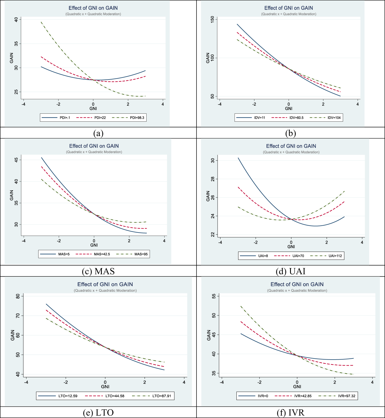
Table 4 also provides the moderating effects of national culture on the GNI–GAIN relationship. In the case of PDI and IVR, the level cross product is negative, and the squared cross product is positive, which means that an increase in these culture traits leads to a steepening of the GNI–GAIN relationship, thus making GAIN more sensitive to GNI changes. For the others (IDV, MAS, UAI and LTO), the level cross product is positive, and the squared cross product is negative, which means that an increase in these culture traits leads to a flattening of the GNI–GAIN relationship, thus making GAIN less sensitive to changes in GNI. Figure 1a shows that with the increase in the PDI, there is a steepening of the GNI–GAIN curve. Figure 1b shows the flattening effect of IDV on the GNI–GAIN curve. Figure 1c shows that MAS also flattens the GNI–GAIN curve. Figure 1d shows that the flattening effect of UAI also increases the positive effects of GNI on GAIN. Figure 1e shows the flattening effect of LTO on the GNI–GAIN curve. Figure 1f shows the steepening effect of IVR on the GNI–GAIN curve.
Moderating effects of: (a) PDI, (b) IDV, (c) MAS, (d) UAI, (e) LTO and (f) IVR.

Figure 1 Long description
A line graph titled, Effect of GNI on GAIN, with subtitle, Quadratic x plus Quadratic Moderation. X axis label GNI with tick labels negative 4, negative 2, 0, 2, 4. Y axis label GAIN with tick labels 25, 30, 35, 40. Legend shows three series: PDI equals negative 1 shown as a solid line, PDI equals 22 shown as a dashed line and PDI equals 98.3 shown as a dashed line with longer dash spacing. All three series form a curved shape with a low point near GNI around 0. The PDI equals 98.3 line is highest near GNI around negative 3 at about GAIN around 40, then drops to about GAIN around 25 by GNI around 2 to 3. The PDI equals negative 1 and PDI equals 22 lines are near GAIN around 30 to 32 at GNI around negative 3, dip to around GAIN around 27 near GNI around 0, then rise slightly by GNI around 3. The image B showing a line graph titled, Effect of GNI on GAIN, with subtitle, Quadratic x plus Quadratic Moderation. X axis label GNI with tick labels negative 4, negative 2, 0, 2, 4. Y axis label GAIN with tick labels 50, 100, 150. Legend shows three series: IDV equals 11 shown as a solid line, IDV equals 60.5 shown as a dashed line and IDV equals 104 shown as a dashed line with longer dash spacing. All three series slope downward from left to right. Near GNI around negative 3, the solid line is around GAIN around 140, the dashed line is around GAIN around 130 and the longer dash line is around GAIN around 120. The three lines converge and cross near GNI around 0 at about GAIN around 90. Near GNI around 3, the solid line is around GAIN around 50, the dashed line is around GAIN around 55 and the longer dash line is around GAIN around 60. The image C showing a line graph titled, Effect of GNI on GAIN, with subtitle, Quadratic x plus Quadratic Moderation. X axis label GNI with tick labels negative 4, negative 2, 0, 2, 4. Y axis label GAIN with tick labels 30, 35, 40, 45. Legend shows three series: MAS equals 5 shown as a solid line, MAS equals 42.5 shown as a dashed line and MAS equals 95 shown as a dashed line with longer dash spacing. All three series slope downward from left to right and flatten toward the right side. Near GNI around negative 3, the solid line is around GAIN around 45, the dashed line is around GAIN around 43 and the longer dash line is around GAIN around 40. The lines come close near GNI around 0 at about GAIN around 35. Near GNI around 3, the solid line is around GAIN around 28 to 29, the dashed line is around GAIN around 29 to 30 and the longer dash line is around GAIN around 30. The image D showing a line graph titled, Effect of GNI on GAIN, with subtitle, Quadratic x plus Quadratic Moderation. X axis label GNI with tick labels negative 4, negative 2, 0, 2, 4. Y axis label GAIN with tick labels 22, 24, 26, 28, 30. Legend shows three series: UAI equals 8 shown as a solid line, UAI equals 70 shown as a dashed line and UAI equals 112 shown as a dashed line with longer dash spacing. The solid line forms a U shaped curve, starting near GNI around negative 3 at about GAIN around 30, dropping to a low near GNI around 1 at about GAIN around 23, then rising to about GAIN around 24 by GNI around 3. The dashed and longer dash lines also curve upward on the right side, with values near GNI around 3 around GAIN around 25 to 27 and they are closer to GAIN around 24 to 25 near GNI around 0. The image E showing a line graph titled, Effect of GNI on GAIN, with subtitle, Quadratic x plus Quadratic Moderation. X axis label GNI with tick labels negative 4, negative 2, 0, 2, 4. Y axis label GAIN with tick labels 40, 50, 60, 70, 80. Legend shows three series: LTO equals 12.59 shown as a solid line, LTO equals 44.58 shown as a dashed line and LTO equals 87.91 shown as a dashed line with longer dash spacing. All three series slope downward from left to right. Near GNI around negative 3, the solid line is around GAIN around 75, the dashed line is around GAIN around 72 and the longer dash line is around GAIN around 68. The lines converge near GNI around 0 at about GAIN around 55. Near GNI around 3, the solid line is around GAIN around 42, the dashed line is around GAIN around 44 and the longer dash line is around GAIN around 46. The image F showing a line graph titled, Effect of GNI on GAIN, with subtitle, Quadratic x plus Quadratic Moderation. X axis label GNI with tick labels negative 4, negative 2, 0, 2, 4. Y axis label GAIN with tick labels 35, 40, 45, 50, 55. Legend shows three series: IVR equals 0 shown as a solid line, IVR equals 42.85 shown as a dashed line and IVR equals 97.32 shown as a dashed line with longer dash spacing. All three series slope downward from left to right and flatten toward the right side. Near GNI around negative 3, the solid line is around GAIN around 45, the dashed line is around GAIN around 48 and the longer dash line is around GAIN around 52. The lines come close near GNI around 0 at about GAIN around 40. Near GNI around 3, the solid line is around GAIN around 38 to 39, the dashed line is around GAIN around 37 and the longer dash line is around GAIN around 35. Across all six graphs, the x axis is GNI with the same tick labels negative 4 to 4 and the y axis is GAIN. Images B, C, E and F show mostly downward sloping lines as GNI increases, while images A and D show curved lines with a low point near GNI around 0 to 1. Each graph compares three moderator levels using solid, dashed and longer dash line styles.
Table 5 shows the short-run estimates of the Panel Quantile ARDL model. The ECM-1 variable shown in this table represents the convergence coefficient. Since it is negative and significant in all cases, it shows that the model is converging, and the independent variables can be used for intervention to increase GAIN, while other variables like INST and REN have a positive effect on GAIN in the short run.
Panel quantile regression model short-run estimates

Table 5 Long description
Short-run panel quantile regression estimates are reported for six cultural outcomes: power distance, individualism, masculinity, uncertainty avoidance, long-term orientation, and indulgence. Institutional change has a consistently strong positive coefficient in every equation, about 1.04 to 1.16, with very small probabilities indicating high statistical significance. The error-correction term is negative in all models, about minus 0.02 to minus 0.024, and is statistically significant, suggesting adjustment toward a long-run relationship. Income change and the squared-income change show mixed signs across outcomes and have large probabilities, indicating they are not statistically significant in these short-run estimates. Interaction terms between income and culture, and between squared income and culture, are near zero and not statistically significant across all outcomes. Renewable energy change is positive and statistically significant for power distance, individualism, masculinity, and uncertainty avoidance, but not significant for long-term orientation or indulgence. Population density change and carbon dioxide change are not statistically significant in any equation. Sample size is 1,033 for the first four outcomes and 1,198 for long-term orientation and indulgence, covering 53 countries, with pseudo R squared values around 0.048 to 0.059, so overall explanatory power is modest.
Standard errors in square brackets. Probability in parentheses.
Source: Authors’ construction.
Supplementary Appendix Table A5 showing panel dynamic GMM estimates provides robustness against possible endogeneity and instrumental variable GMM (Supplementary Appendix Table A6) which is robust to endogeneity and cross-sectional dependence. While comparing the results, it can be noted that the direction of estimates for controlling variables is similar for all the models, but while comparing the estimates of GNI and the moderating effects, the results match with the baseline panel quantile ARDL model for models of PDI, IDV, MAS and IVR. In the case of UAI and LTO, the results slightly differ, showing that, in these cases, higher GNI deteriorates climate change adaptability, while UA and long-term orientation help to restore the adaptability.
5. Conclusion and discussion
This study explored Hofstede’s six national culture index variables to see how they interacted and modulated the demand-based EKC relationship. This is based on the idea that culture influences how people set their demand patterns in terms of how they adapt to climate change and their environmental impact. The culture index has two separate implications in this context. The first set of culture variables has the potential to transform the U-shaped demand EKC, which is moderated by culture variables. This confirms that the demand-motivated adaptation is conditioned by national culture. This study includes contextual controls like institutional quality, carbon intensity, renewable energy and population density.
This study provided several important insights. The results confirm the non-linear income-to-adaptation relationship as U-shaped. The study suggests that policymakers who pursue higher GNI can motivate adaptive behaviours in populations, but GNI is required to pass a certain threshold. The findings also confirm that national culture is important in identifying the income-adaptation pathway. Culture moderates the curvature of this relationship. Hence, societies with different cultural orientations may experience mature adaptation promoting income levels at different speeds. Culture is presented as an institutional force that can shape household consumption and saving patterns that can ensure adaptability.
Several policy implications for governments, international developmental agencies and adaptation planners were provided. Climate adaptation does not grow linearly with income, and the U-shaped effect indicates that a certain demand force that can motivate a national-level improvement in adaptability must be developed. This high level of GNI would help in altering consumer low-carbon choices, energy consumption transition and boosting climate-aware investments. Institutions are also important pillars in boosting adaptability by supporting climate finance, renewable energy projects, disaster-risk planning and resilient infrastructure. Better institutions help in providing long-term policy commitments and conducive environments. Culture policies are culture-sensitive. Global-level efforts to boost climate change resilience must also consider the cultural differences among societies. Efforts like participatory mechanisms, community-based adaptation programs, incentive-based mechanisms, promotion of intergenerational investments and immediate gain determination can help to align GNI towards climate-adaptive economies.
In conclusion, while estimating a generalized model, this study also provides context-specific estimates, as one-size does not fit all. Policymakers can find the effectiveness of independent variables with respect to the quantile position of adaptation levels. Furthermore, GNI and culture-specific effects are also provided by this model. The model can therefore address diversity within the generalized model.
Supplementary material
The supplementary material for this article can be found at https://doi.org/10.1017/S1355770X26100758.
Competing interests
The authors declare none.




 Open access

