



1 Introduction
The oscillatory boundary layer has been the subject of several theoretical, experimental and numerical studies because of its relevance to fluid flow phenomena of practical interest ranging from unsteady flow in pipes to oscillatory flows in the natural environment. One of the first experimental studies to investigate oscillatory boundary layer in detail is that of Jonsson & Carlsen (Reference Jonsson and Carlsen1976), who measured velocities, but not turbulence, within the boundary layer for high Reynolds number
 $O$
(
 $10^{6}$
) sinusoidal oscillatory flows over rough beds in a large oscillatory flow tunnel. Here the Reynolds number is
 $Re=\tilde{u} _{0max}a/\unicode[STIX]{x1D708}$
, where
 $\tilde{u} _{0max}$
is the maximum free-stream horizontal oscillatory velocity,
 $a$
is the amplitude of free-stream water particle excursion and
 $\unicode[STIX]{x1D708}$
is the kinematic viscosity. Hino, Sawamoto & Takasu (Reference Hino, Sawamoto and Takasu1976) experimentally investigated the transition to turbulence of oscillatory flow in an oscillatory wind tunnel facility and later studied the turbulence structure of the flow (Hino et al.
Reference Hino, Kashiwayanagi, Nakayama and Hara1983). Subsequent work by Sleath (Reference Sleath1987) for sinusoidal flows with
 $Re\approx 3\times 10^{5}$
over rough beds and by Jensen, Sumer & Fredsøe (Reference Jensen, Sumer and Fredsøe1989) for sinusoidal flows with
 $7.5\times 10^{3}\leqslant Re\leqslant 6\times 10^{6}$
over smooth and rough beds, yielded measures of phase-averaged velocities, boundary layer thickness, flow phase lead and turbulence generation and dissipation at each phase of the flow cycle. For a smooth wall, Jensen et al. (Reference Jensen, Sumer and Fredsøe1989) showed that there are phases in the flow cycle when the flow is not fully turbulent, even for
 $Re$
as high as
 $1.6\times 10^{6}$
, and that a logarithmic velocity profile develops after some time following flow reversal, which persists far into the decelerating stage of the flow following peak free-stream velocity. More recent experimental work includes Carstensen, Sumer & Fredsøe’s (Reference Carstensen, Sumer and Fredsøe2010) flow tunnel measurements of the onset of turbulence, marked by the emergence of turbulent spots close to a smooth wall, and the high Reynolds number (
 $Re~O(10^{6})$
) studies of van der A et al. (Reference van der A, O’Donoghue, Davies and Ribberink2011) involving asymmetric flows over rough beds and Yuan & Madsen (Reference Yuan and Madsen2014) involving sinusoidal, skewed and asymmetric flows over smooth and rough beds. The variations in flow shape from sinusoidal flow in the latter two studies were motivated by the need to understand boundary layer hydrodynamics occurring under sea waves, for which the near-bed oscillatory flow is generally skewed and asymmetric, the degree of which depends on the nonlinear transformation of the wave shape as it progresses shoreward. While the combined effort of previous experimental work has substantially advanced understanding of turbulence in oscillatory boundary layer flows, results to date are limited to observations of turbulent fluctuations to second order (turbulence intensity, turbulent kinetic energy and Reynolds stresses), with, to the authors’ knowledge, no results thus far for the higher-order turbulence statistics, which are important to characterise properly the turbulent flow.
Direct numerical simulations (DNSs) of turbulent oscillatory boundary layer over a smooth wall were performed by Spalart & Baldwin (Reference Spalart, Baldwin, Durst, Launder, Schmidt and Whitelaw1989), who reported phase-averaged velocity profiles and second-order turbulence statistics. The role of wall imperfections in triggering the flow instability in an oscillatory boundary layer was examined by Blondeaux & Vittori (Reference Blondeaux and Vittori1994). Numerical simulations were also performed by Vittori & Verzicco (Reference Vittori and Verzicco1998) with the focus on explaining the mechanisms involved in the transition to turbulence. The authors showed that wall imperfections may play an important role in triggering the flow instability. The role of wall imperfections has been further examined by Costamagna, Vittori & Blondeaux (Reference Costamagna, Vittori and Blondeaux2003) and Mazzuoli, Vittori & Blondeaux (Reference Mazzuoli, Vittori and Blondeaux2011), who reproduced two experiments of Carstensen et al. (Reference Carstensen, Sumer and Fredsøe2010), and most recently by Scandura (Reference Scandura2013), who proved that wall imperfections are crucial in triggering the appearance of the vortex tubes studied experimentally by Carstensen et al. (Reference Carstensen, Sumer and Fredsøe2010). The effect of Reynolds number and initial velocity condition on the transition to turbulence have been analysed by Ozdemir, Hsu & Balachandar (Reference Ozdemir, Hsu and Balachandar2014). The tests of Jensen et al. (Reference Jensen, Sumer and Fredsøe1989) have been reproduced numerically by Salon, Armenio & Crise (Reference Salon, Armenio and Crise2007) and by Pedocchi, Cantero & Garcia (Reference Pedocchi, Cantero and Garcia2011). Both found reasonably good agreement in terms of the profiles of the turbulent statistics but poor agreement in terms of the second-order statistics of the wall shear stress. More recently, Scandura, Faraci & Foti (Reference Scandura, Faraci and Foti2016) performed DNSs focused on the time development of the wall shear stress statistics for asymmetric (i.e. acceleration-skewed) oscillatory flows over a smooth wall. They showed that peaks in the higher-order statistics of the wall shear stress are associated with the development of low-speed streaks: the higher-order statistics are maximum at the onset of breaking of the low-speed streaks and rapidly decrease thereafter, becoming approximately constant when breaking has occurred across the entire flow domain. The high-order statistical analysis performed by Scandura et al. (Reference Scandura, Faraci and Foti2016) involved the wall shear stress only. As is the case for experimental studies, no DNS results have been reported to date for the higher-order velocity statistics and the probability density distributions of the velocity fluctuations.
Present knowledge of higher-order statistics for wall-bounded flows originates from studies of steady turbulent channel flows, pipe flows and boundary layer flows. A short summary of key results from these works is presented here. Wei & Willmarth (Reference Wei and Willmarth1989) carried out laser-Doppler anemometry (LDA) measurements in a steady turbulent channel flow and reported a relative intensity of the streamwise velocity fluctuations (
 $\langle {u^{\prime }}^{2}\rangle ^{1/2}/\langle u\rangle$
) of approximately 0.25 in the near-wall region; no results were reported for the skewness or flatness. Alfredsson et al. (Reference Alfredsson, Johansson, Haritonidis and Eckelmann1988) made hot-wire and hot-film measurements of near-wall velocities in an oil channel and a wind tunnel. They report a limiting value of approximately 0.4 for the relative intensity
 $\langle u^{\prime 2}\rangle ^{1/2}/\langle u\rangle$
as the wall is approached in the case of oil flow and approximately 0.1 in the case of the wind flow; the
 $u^{\prime }$
skewness (
 $\langle {u^{\prime }}^{3}\rangle /\langle {u^{\prime }}^{2}\rangle ^{3/2}$
) and flatness (
 $\langle {u^{\prime }}^{4}\rangle /\langle {u^{\prime }}^{2}\rangle ^{2}$
) asymptotically approached values of approximately 1 and 4.8 respectively close to the wall. Barlow & Johnston (Reference Barlow and Johnston1985) carried out LDA measurements in a steady turbulent boundary layer over a flat and a concave surface and found little difference between the flow statistics close to the two types of surface. They report a
 $u^{\prime }$
relative intensity of approximately 0.4 near the wall, decreasing to 0.12 for
 $y^{+}=50$
. The skewness of
 $u^{\prime }$
was about 1 near the wall, changing sign at
 $y^{+}=15$
and reaching about
 $-0.4$
at
 $y^{+}=50$
. In these experiments the flatness of
 $u^{\prime }$
appears to approach a value of approximately 5 as the wall is approached, although the trend is not entirely clear. Near-wall measurements in a rectangular duct by Kreplin & Eckelmann (Reference Kreplin and Eckelmann1979) showed similar
 $u^{\prime }$
statistics as Barlow & Johnston (Reference Barlow and Johnston1985), but the skewness of the vertical velocity component showed significant differences. Durst, Jovanovic & Sender (Reference Durst, Jovanovic and Sender1995) carried out LDA measurements in a turbulent pipe flow and reported
 $u^{\prime }$
and
 $v^{\prime }$
relative intensities of 0.36 and zero respectively;
 $u^{\prime }$
skewness and flatness values are 0.85 and 4.1 respectively as the wall is approached, values which are consistent with previous measurements and with numerical simulations for turbulent channel flows reported by Kim, Parviz & Robert (Reference Kim, Parviz and Moser1987). However, Durst et al.’s (Reference Durst, Jovanovic and Sender1995) near-wall
 $v^{\prime }$
flatness is substantially different from that shown in Kim et al. (Reference Kim, Parviz and Moser1987). In particular, Durst et al. (Reference Durst, Jovanovic and Sender1995), like Kreplin & Eckelmann (Reference Kreplin and Eckelmann1979) and Barlow & Johnston (Reference Barlow and Johnston1985) previously, showed that
 $v^{\prime }$
flatness decreases as the wall is approached, while Kim et al. (Reference Kim, Parviz and Moser1987) showed that it increases. A decrease in
 $v^{\prime }$
flatness is also reported by Karlsson & Johansson (Reference Karlsson, Johansson and Adrian1986), although their values of near-wall
 $v^{\prime }$
flatness are significantly higher than those reported in the other studies.
Information of the higher-order statistics is relevant for practical modelling of sediment transport, which is one of the motivations behind the present work. To recognise the random nature of turbulence and the intermittency of turbulent flow structures that transport high momentum fluid towards the bed, stochastic models for the initiation of sediment motion have been developed, which take into account the probability density of the bed shear stress (e.g. Hofland & Battjes Reference Hofland and Battjes2006). Practical two-phase models, in which the fluid phase is modelled using a turbulence-averaged approach, include the effect of the velocity fluctuations on the particle dispersion through a stochastic model for the velocity fluctuations. This approach has recently lead to encouraging results for steady-flow suspended sediment (Shi & Yu Reference Shi and Yu2015) and sheet flow transport (Cheng et al. Reference Cheng, Chauchat, Hsu and Calantoni2018). However, the majority of these stochastic models assume a normal distribution of turbulent fluctuations which, based on the previously mentioned experimental studies, does not hold for steady flows.
Compared to steady flows, information on high-order statistics is currently lacking for turbulent oscillatory boundary layer flows. This is likely due to the far greater effort required in terms of measurements and simulations to achieve convergence of the statistics. The present paper aims to address this lack of knowledge. We report on a combined experimental–numerical study of oscillatory flows over a smooth wall, which has yielded low- and high-order turbulence statistics, in addition to results for mean velocity and Reynolds stress, providing a complete characterisation of the turbulent flow. The flow velocity is asymmetric, which adds to the richness of the results (compared to a sinusoidal flow) because the difference in flow acceleration between the positive and negative flow half-cycles leads to differences in half-cycle turbulence behaviour. Also, choosing an asymmetric flow allows us to build on the previous DNS work of Scandura et al. (Reference Scandura, Faraci and Foti2016), which focused on wall shear stress, not on the turbulent velocity statistics. The experiments cover a wide range of
 $Re$
, enabling examination of the effect of
 $Re$
on the flow and turbulence statistics. DNS is performed for the lower-
 $Re$
flows, which are numerically more achievable, and DNS results are used to explore aspects of the flow that cannot be measured in the experiments. The flow Reynolds numbers and asymmetry parameters for the study fall within those observed under full-scale waves in the field.
Section 2 describes the experimental facility, the instrumentation and the test conditions. The DNS approach and set-up is described in § 3. Section 4 constitutes the main body of the paper, presenting a comparison between the experimental and numerical results and detailed analyses and discussion of the turbulence statistics. The key findings are summarised in § 5.
2 Experiments
2.1 Test facility
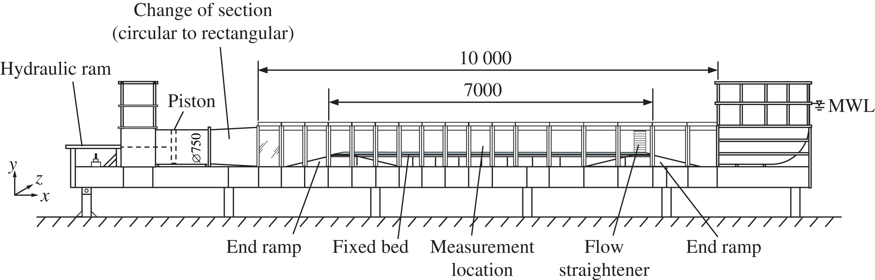
The Aberdeen oscillatory flow tunnel (AOFT, figure 1) is a large laboratory facility in which near-bed horizontal flows, equivalent in period and amplitude to the near-bed flows beneath full-scale waves, can be generated. In tunnels of this kind the flow is driven through a closed rectangular section conduit. There is no free water surface in the test section, which means that the oscillatory flow differs from that generated by surface waves in having zero vertical orbital motion in the free stream and being horizontally uniform. The AOFT is of U-tube construction with an overall length of 16 m, 10 m of which is a glass-sided rectangular test section, 0.75 m high and 0.3 m wide. Open reservoirs at either end of the tunnel accommodate the volume of water displaced by the horizontally driven piston. The 1 m diameter piston is housed in a circular cylindrical section at one end of the tunnel and is electro-hydraulically controlled within a closed-loop feedback system. The circular piston section is linked to the rectangular test section by a 1 m long change of section.
For the present study the test section was fitted with a 7 m long raised false floor consisting of a stainless steel framework with 25 mm thick PVC panels elevated to 0.25 m above the tunnel floor. At both ends ramps were fitted with 1:4 slopes from the tunnel floor to the horizontal false bottom. A 7 m long, 20 mm thick acrylic smooth bed, comprising a middle 3 m long section and 2 m long section on each side, was attached to the false floor with countersunk bolts. The bolt holes in the central panel and the joins between the panels were covered with epoxy resin to provide a smooth surface and limit flow disturbance; the bolt holes on the two remaining panels were covered with acrylic type. As a result of the raised floor the water depth in the tunnel test section was 0.48 m. The
 $x,y,z$
-coordinate system used throughout this paper has its origin in the longitudinal centre of the test section, at the intersection between the bed and the glass wall on the side where the LDA laser beams entered the test section. The
 $x$
-axis is the streamwise direction and is positive towards the open-ended riser, the
 $y$
-axis is normal to the bottom wall and is positive upwards, the
 $z$
-axis is the spanwise direction and is positive into the test section. The velocity components along the
 $x$
,
 $y$
and
 $z$
axes are denoted
 $u$
,
 $v$
and
 $w$
respectively.
The experimental facility.
2.2 Instrumentation
Velocity measurements were made with a backscatter LDA system (Dantec FibreFlow), consisting of a 112 mm diameter probe, a 300 mW air-cooled Ar-Ion laser and a Dantec F60 Burst Spectrum Analyser. The probe was fitted with a 310 mm focal length (in air) lens, resulting in an ellipsoidal measurement volume with a maximum diameter of
 $47~\unicode[STIX]{x03BC}\text{m}$
and a length of
 $530~\unicode[STIX]{x03BC}\text{m}$
in the spanwise direction. The probe was attached to a computer-controlled stepper-motor driven traverse, allowing the probe to be positioned in the
 $x$
,
 $y$
and
 $z$
directions with a resolution of
 $12.5~\unicode[STIX]{x03BC}\text{m}$
(full step). To check the accuracy of the traverse
 $y$
-positioning, a confocal chromatic displacement sensor (Micro-Epsilon ConfocalDT IFS2405-10, range 10 mm with sub-
 $\unicode[STIX]{x03BC}\text{m}$
resolution) monitored the displacement of the traverse when the LDA measurement volume was within the first 10 mm above the wall. This measurement confirmed that the traverse positioning was accurate to within
 $10~\unicode[STIX]{x03BC}\text{m}$
.
The LDA system was used in two different configurations. First, the system was set up in one-component mode to measure only the streamwise velocity component close to the wall (
 $y\leqslant 0.3$
mm). This set-up allowed the laser beams to be oriented parallel to the bed, thereby minimising the wall-normal coverage of the measurement volume. These measurements were made at 60 mm from the glass side wall (
 $z=60$
mm) to reduce the travel distance of the laser beams through the water in order to improve the backscattered signal and, hence, the data rates (typically
 ${\sim}100~\text{Hz}$
). The seeding for these near-wall measurements consisted of
 $10~\unicode[STIX]{x03BC}\text{m}$
silver-coated hollow glass spheres (specific gravity 1.6). Velocity measurements were typically made at
 $y=0.1$
, 0.15, 0.2 and 0.3 mm for a duration of 500 flow cycles at each elevation. Below 0.1 mm accurate measurements could not be made due to the reflections from the wall. The vertical position of the measurement volume relative to the wall was determined by traversing the centre of the measurement volume vertically onto a
 $5~\unicode[STIX]{x03BC}\text{m}$
diameter tungsten wire which was placed at a known distance (measured by the confocal displacement sensor) parallel to the wall (similar to the approach used by Durst, Müller & Jovanovic Reference Durst, Müller and Jovanovic1988).
For the remaining measurements the system was set up in two-component configuration, measuring the two velocity components at
 $45^{\circ }$
to the streamwise direction. In order to measure close to the wall (0.2 mm) in this configuration the probe was tilted forward by
 $3^{\circ }$
which prevented the bottom two laser beams being optically blocked by the acrylic bed. As a result the vertical velocity component was not truly wall-normal but tilted
 $3^{\circ }$
from the normal. Profile measurements were made at
 $z=125$
mm, typically over 25 vertical points logarithmically spaced between 0.2 mm and 250 mm above the wall. In this set-up the wall was located by traversing the measurement volume into the wall. The zero position corresponds to the position of the maximum backscattered light intensity, caused by the scattering of small particles attached to the wall surface. The measurement duration was 200 cycles for elevations close to the wall, reducing to 100 cycles for elevations far away from the wall. Seeding particles for these measurements consisted of
 $15~\unicode[STIX]{x03BC}\text{m}$
silver-coated hollow glass spheres (s.g. 1.0). These seeding particles, like the
 $10~\unicode[STIX]{x03BC}\text{m}$
seeding used for the very near-wall measurements, can be expected to follow the flow faithfully since the particle Stokes number is
 $\ll 1$
.
Synchronisation between the piston position and the LDA system was achieved by sending a once-per-flow-cycle signal to the LDA system, which allows phase-averaging of the velocity measurements (§ 2.3). In addition, the input and measured piston displacements were recorded on the LDA system simultaneously with the velocity measurements, allowing post-experiment confirmation of the synchronisation.
2.3 Data processing
Accounting for particle residence time weighting (e.g. Buchhave, George & Lumley Reference Buchhave, George and Lumley1979) the phase-averaged streamwise velocity is determined as follows:
 $$\begin{eqnarray}\langle u\rangle (y,\unicode[STIX]{x1D70E}t)=\frac{\displaystyle \mathop{\sum }_{j=1}^{N}\displaystyle \mathop{\sum }_{i=1}^{M}u_{i}(y,\unicode[STIX]{x1D719}+(j-1)2\unicode[STIX]{x03C0})tt_{i}(y,\unicode[STIX]{x1D719}+(j-1)2\unicode[STIX]{x03C0})}{\displaystyle \mathop{\sum }_{j=1}^{N}\displaystyle \mathop{\sum }_{i=1}^{M}tt_{i}(y,\unicode[STIX]{x1D719}+(j-1)2\unicode[STIX]{x03C0})}\quad \text{for }0\leqslant \unicode[STIX]{x1D70E}t<2\unicode[STIX]{x03C0},\end{eqnarray}$$
where
 $N$
is the number of flow cycles at a given elevation,
 $\unicode[STIX]{x1D719}$
is the phase window or phase ‘bin’
 $\unicode[STIX]{x1D70E}t\leqslant \unicode[STIX]{x1D719}<\unicode[STIX]{x1D70E}t+\unicode[STIX]{x0394}\unicode[STIX]{x1D70F}$
,
 $M$
is the total number of samples in a given phase bin and
 $tt_{i}$
the duration for a seeding particle to traverse the measurement volume. The size of the phase bin is obtained from
 $\unicode[STIX]{x0394}\unicode[STIX]{x1D70F}=2\unicode[STIX]{x03C0}/(f_{s}T)$
where
 $f_{s}$
is a pre-defined sampling rate, here set to
 $f_{s}=50~\text{Hz}$
. The turbulent fluctuation is defined as
 $u^{\prime }=u-\langle u\rangle$
, where the phase-averaged velocity,
 $\langle u\rangle$
, consists of a time-averaged component,
 $\bar{u}$
, and an oscillatory component,
 $\tilde{u}$
, i.e.
 $\langle u\rangle =\bar{u}+\tilde{u}$
. The streamwise root-mean-square velocity fluctuations are given by (for
 $0\leqslant \unicode[STIX]{x1D70E}t<2\unicode[STIX]{x03C0}$
):
 $$\begin{eqnarray}\sqrt{\langle {u^{\prime }}^{2}\rangle (y,\unicode[STIX]{x1D70E}t)}=\sqrt{\frac{\displaystyle \mathop{\sum }_{j=1}^{N}\displaystyle \mathop{\sum }_{i=1}^{M}(u_{i}(y,\unicode[STIX]{x1D719}+(j-1)2\unicode[STIX]{x03C0})-\langle u\rangle (y,\unicode[STIX]{x1D70E}t))^{2}tt_{i}(y,\unicode[STIX]{x1D719}+(j-1)2\unicode[STIX]{x03C0})}{\displaystyle \mathop{\sum }_{j=1}^{N}\displaystyle \mathop{\sum }_{i=1}^{M}tt_{i}(y,\unicode[STIX]{x1D719}+(j-1)2\unicode[STIX]{x03C0})}}.\end{eqnarray}$$
Analogous equations were applied to calculate the higher-order moments of the velocity fluctuations
 $\langle {u^{\prime }}^{3}\rangle$
and
 $\langle {u^{\prime }}^{4}\rangle$
, to obtain the statistics of the wall-normal velocity component
 $v$
and to obtain the Reynolds shear stress
 $\langle u^{\prime }v^{\prime }\rangle$
. The transit time weighting correction accounts for temporal velocity bias in the measurements, however its effect was only noticeable at phases of low velocity around flow reversal.
Any outliers in the data set can lead to significant errors in the higher-order statistics. During acquisition the burst signals were monitored for their quality based on a signal-to-noise ratio (SNR), defined as the ratio of the highest correlation peak compared to the second highest correlation peak in a burst. A velocity measurement with SNR below a certain threshold is rejected. For the present experiment the SNR threshold was set to values as high as 10–14 (particularly for the near-wall measurements) which meant that the recorded velocity data were practically free of any outliers. Any remaining outliers were removed during post-processing by rejecting velocity measurements in a certain phase bin that deviated more than
 $\pm 8$
standard deviations from the median velocity in that phase bin. This detection threshold was determined by comparing the results with the DNS simulations, and is similar to the range of
 $\pm 7$
standard deviations used by Durst et al. (Reference Durst, Jovanovic and Sender1995). The number of outliers removed in this way was
 ${\leqslant}0.01\,\%$
of the sampled data.
Experimental conditions, measured at
 $y=84$
mm. Orbital amplitude
 $a$
is determined
 $a=\tilde{u} _{0max}/\unicode[STIX]{x1D70E}$
. Reynolds number,
 $R_{\unicode[STIX]{x1D6FF}}$
, was based on kinematic viscosity
 $\unicode[STIX]{x1D708}=1.029\times 10^{-6}~\text{m}^{2}~\text{s}^{-1}$
, based on the average measured water temperature during the experiments.

2.4 Test conditions
The piston displacement was programmed to produce an oscillatory flow in the test section following the description of Abreu et al. (Reference Abreu, Silva, Sancho and Temperville2010). Test conditions consisted of five asymmetric oscillatory flows with a constant flow period of
 $T=7$
s, but different Reynolds number
 $R_{\unicode[STIX]{x1D6FF}}$
(see table 1). Here
 $R_{\unicode[STIX]{x1D6FF}}=\tilde{u} _{0max}\unicode[STIX]{x1D6FF}/\unicode[STIX]{x1D708}$
, where
 $\tilde{u} _{0max}$
is the maximum of the oscillatory component of the free-stream velocity, and
 $\unicode[STIX]{x1D6FF}$
is the Stokes length given by
 $\sqrt{2\unicode[STIX]{x1D708}/\unicode[STIX]{x1D70E}}$
, with
 $\unicode[STIX]{x1D708}$
the kinematic viscosity and
 $\unicode[STIX]{x1D70E}=2\unicode[STIX]{x03C0}/T$
.
The degree of free-stream velocity skewness and asymmetry are defined as
 $$\begin{eqnarray}\displaystyle & \displaystyle Sk=\frac{\overline{(\tilde{u} _{0})^{3}}}{(\overline{\tilde{u} _{0}^{2}})^{3/2}}, & \displaystyle\end{eqnarray}$$
 $$\begin{eqnarray}\displaystyle & \displaystyle Asy=\frac{\overline{\mathscr{H}(\tilde{u} _{0})^{3}}}{(\overline{\tilde{u} _{0}^{2}})^{3/2}}, & \displaystyle\end{eqnarray}$$
where subscript 0 indicates free-stream elevations and
 $\mathscr{H}$
is the Hilbert transform of
 $\tilde{u} _{0}$
.
The target oscillatory flow conditions were designed to have the same degree of asymmetry and zero skewness. However, exact reproducibility of the target flow is not always possible in the test section. Nevertheless, table 1 shows that the differences in the measured skewness and asymmetry are small between the five conditions, so that for comparison purposes the flows can be distinguished solely based on
 $R_{\unicode[STIX]{x1D6FF}}$
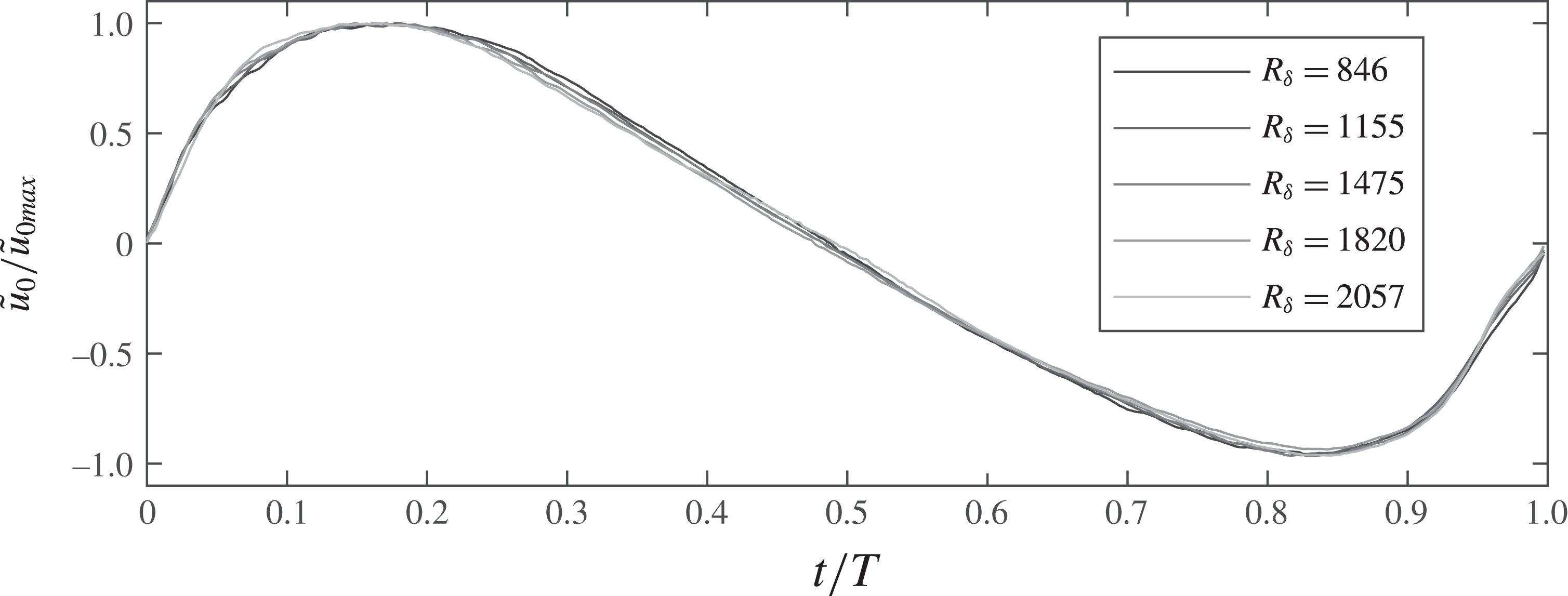
. Figure 2 shows the measured oscillatory component of the free-stream velocity
 $\tilde{u} _{0}$
normalised by the maximum velocity for all five experimental conditions. The agreement between the different conditions is very good, confirming that
 $R_{\unicode[STIX]{x1D6FF}}$
is the only parameter that distinguishes the experiments from each other.
Normalised streamwise velocity measured at
 $y=84$
mm.
3 Direct numerical simulations
For the numerical simulations a Cartesian coordinate system oriented as described in § 2.1 is adopted. The Navier–Stokes equations have been integrated numerically in a domain of size
 $(L_{x},L_{y},L_{z})$
along the
 $x$
,
 $y$
and
 $z$
directions respectively. In order to reproduce the experimental results the flow was driven by a pressure gradient consistent with the velocity measured in the irrotational region. More specifically, the pressure gradient is given by
 $\unicode[STIX]{x1D70C}\text{d}\tilde{u} _{0}/\text{d}t$
, where
 $\tilde{u} _{0}(t)$
denotes the experimental free-stream velocity measured at
 $y=84$
mm shown in figure 2. The numerical approach is based on a second-order finite difference approximation on a staggered grid. The time advancement is carried out by means of the second-order Crank–Nicolson scheme for the viscous terms and by means of a third-order Runge–Kutta scheme for the convective terms. At the wall (
 $y=0$
) a no-slip condition is imposed for all velocity components,
 $(u,v,w)=(0,0,0)$
, and on the upper boundary of the domain (
 $y=L_{y}$
) the following free shear stress condition is imposed
 $(\unicode[STIX]{x2202}u/\unicode[STIX]{x2202}y,v,\unicode[STIX]{x2202}w/\unicode[STIX]{x2202}y=0,0,0)$
. Finally, periodic boundary conditions are introduced in the
 $x$
and
 $z$
directions of the domain. The sizes of the numerical grid in the
 $x$
,
 $y$
and
 $z$
directions are denoted
 $n_{x}$
,
 $n_{y}$
and
 $n_{z}$
respectively. The grid spacing is uniform along the
 $x$
and
 $z$
directions, while along the
 $y$
direction the grid is prescribed by means of a hyperbolic tangent function, resulting in a finer spacing near the wall where large gradients exist. Further details on the numerical approach are reported in Scandura et al. (Reference Scandura, Faraci and Foti2016). Table 2 shows the three flow conditions that have been simulated along with the sizes of the flow domain and the numerical grid.
Set-up of the numerical simulations.

Sufficient size of the computational domain was checked for each flow by computing the spatial autocorrelation function of the streamwise velocity fluctuations along the
 $x$
and
 $z$
directions and ensuring that at half the width of the computational domain the autocorrelation function decays to very small values. The adequacy of the grid resolution was verified from the one-dimensional energy spectra
 $E_{uu}$
,
 $E_{vv}$
and
 $E_{ww}$
computed both along the
 $x$
and
 $z$
directions, which showed that the energy at high wavenumbers is at least four orders of magnitude smaller than that at low wavenumbers. Table 2 also shows the numerical resolution in terms of wall units based on the maximum value of the friction velocity. Along the
 $y$
direction the mesh size
 $\unicode[STIX]{x0394}y^{+}$
at the wall is smaller than one half a wall unit, and is therefore sufficient to resolve the viscous sublayer. In the
 $z$
direction the mesh size
 $\unicode[STIX]{x0394}z^{+}$
is approximately six wall units, and is therefore able to resolve the low-speed streaks whose spacing is approximately 100 wall units. The resolution in the
 $x$
direction
 $\unicode[STIX]{x0394}x^{+}$
is smaller than that in the
 $z$
direction but is still sufficient since the turbulent structures are elongated in the streamwise direction. The ensemble averages have been computed by performing first a spatial average over
 $x{-}z$
planes and then a phase average over the number of flow cycles shown in table 2. In § 4.3 the effect of the number of wave cycles on the convergence of the higher-order statistics is demonstrated. Further checks on the reliability of the numerical simulations are shown in the following by comparing the experimental and numerical turbulent statistics.
4 Experimental and numerical results
4.1 Time-averaged and phase-averaged velocities
The asymmetry in the free-stream flow generates an asymmetry in turbulent intensity between the positive and negative flow half-cycles. For this reason, the time-averaged Reynolds stress is not equal to zero. The non-zero mean Reynolds stress in the streamwise mean momentum equation is balanced by a mean viscous stress induced by a steady boundary layer streaming, which has a direction opposite to that of the highest free-stream flow acceleration. While the steady boundary layer streaming is present in both the experiment and numerical simulation, there is a significant difference between vertical profiles of the mean velocity observed in the flow tunnel and numerically. The difference is due to the different boundary conditions applied at the two ends of the fluid domain. More specifically, as shown in figure 1, one end of the tunnel comprises a reservoir in which the flow is free to oscillate up and down, while the other end is bound by the piston which generates the oscillatory flow. Given these boundary conditions the time-averaged flow rate through any cross-section of the facility must be zero to conserve mass. This condition is satisfied by a return current whose flow direction is opposite to that of the steady boundary layer streaming generated by the non-zero mean Reynolds stress, the velocity profile of which depends on the geometry of the tunnel cross-section (Gonzalez-Rodriguez & Madsen Reference Gonzalez-Rodriguez and Madsen2011). On the other hand, in the numerical simulations periodic boundary conditions are applied along the streamwise direction, which do not impose a kinematic constraint on the mean flow rate, and so no return current takes place. In order to reproduce numerically the mean flow observed experimentally, the DNS would need to be performed on a fluid domain delimited by the four tunnel walls, thus covering the cross-sectional area of the test section, which would entail huge computational cost.
Time-averaged streamwise velocities (a) and time-averaged Reynolds stress (b). DNS (line), experiment (dots).

Since the steady boundary layer streaming is driven by the Reynolds stress, the streaming itself does not exert a mean force on the wall (see e.g. Scandura Reference Scandura2007). On the other hand, the return current that occurs in the flow tunnel is driven by a pressure gradient, and therefore the overall flow applies a mean force on the wall in the opposite direction to the boundary layer streaming. Figure 3(a) shows the time-averaged streamwise velocity profiles for both the numerical simulations and the experiments (note that DNS was only performed for the lowest three
 $R_{\unicode[STIX]{x1D6FF}}$
). It can be observed that in the numerical simulations the steady streaming is in the negative streamwise direction and that the
 $y$
-derivative becomes zero at
 $y=0$
, which demonstrates that the mean force acting on the wall is zero. The experimental time-averaged velocity profiles on the other hand exhibit a positive gradient at the wall. However, since it was not possible to measure at distances less than 0.2 mm from the wall for the two-component LDA configuration, this characteristic is not apparent for all conditions in figure 3(a). Only for
 $R_{\unicode[STIX]{x1D6FF}}=846$
can the velocity profile be seen to bend towards zero close to
 $y=0$
, indicating that the return current causes a mean positive tangential stress on the wall.
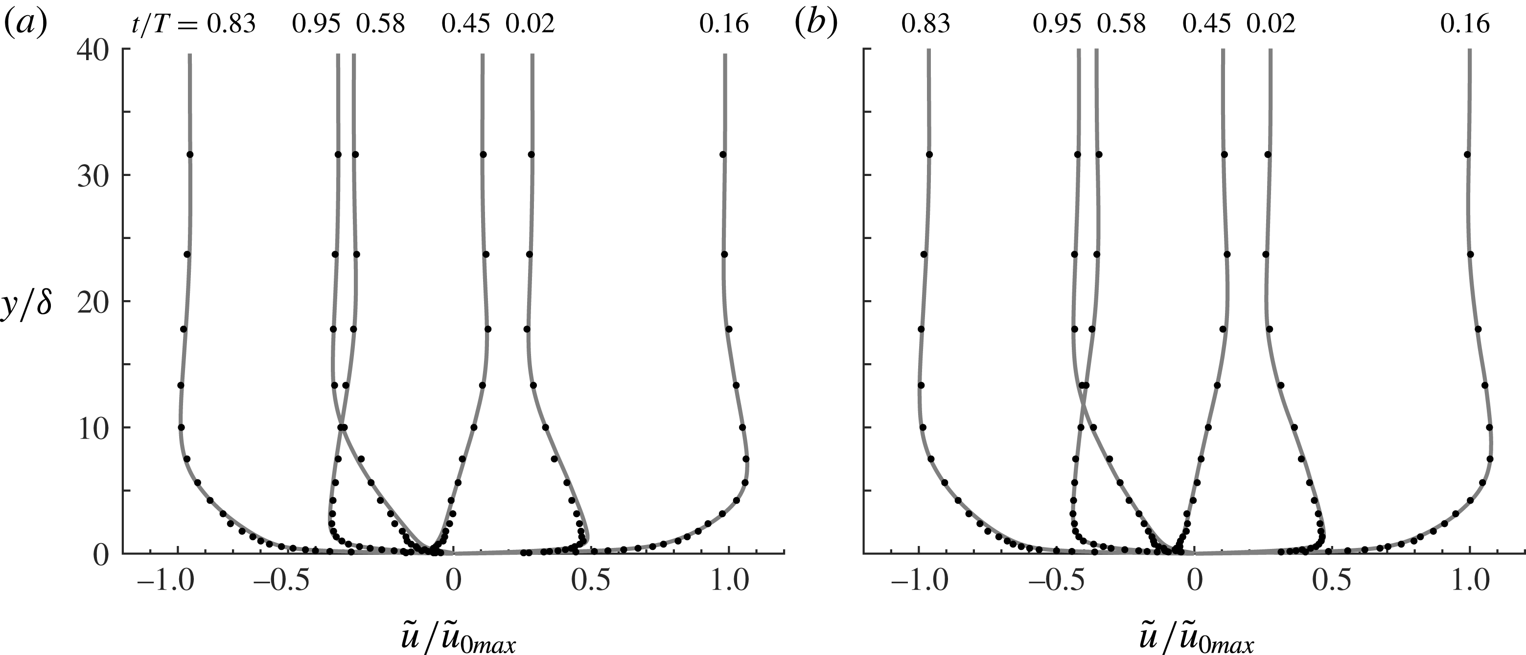
Velocity profile at six phases of the flow cycle for
 $R_{\unicode[STIX]{x1D6FF}}=846$
. (a) Phase-averaged streamwise velocity, (b) oscillatory component of the phase-averaged streamwise velocity. DNS (line), experiment (dots).

In figure 3(b) the measured time-averaged Reynolds shear stresses in the flow tunnel are shown with the corresponding numerical results. Both experiments and simulations show that the mean Reynolds stress is negative near the wall. On the other hand, far from the wall the experiments show a positive mean Reynolds stress while the numerical simulations reduce to zero. This discrepancy is likely due to the gradient of the mean velocity in the oscillatory flow tunnel, which does not vanish far from the wall because of the return flow in the tunnel (figure 3 a).
It might be expected that the difference in the time-averaged velocity profiles between experiments and numerical simulations hinders further comparison between numerical and experimental results. However, since the mean velocity is typically two orders of magnitude lower than the oscillating component, the former has a limited effect on the latter and on the velocity statistics. In fact, very good agreement between the measured and numerical phase-averaged velocity profiles is obtained after the time-averaged velocity is removed. As an example, figure 4 shows a comparison between the velocity profiles at six phases for
 $R_{\unicode[STIX]{x1D6FF}}=846$
, before and after subtracting the mean flow. It can be seen that the agreement improves significantly when the mean flow is removed from both experiments and numerical results, especially near flow reversal when the relative importance of the mean flow is greatest. A similarly good agreement for the oscillatory component of the phase-averaged velocity is observed for
 $R_{\unicode[STIX]{x1D6FF}}=1155$
and
 $R_{\unicode[STIX]{x1D6FF}}=1475$
, as shown in figure 5. In these figures
 $t/T=0.16$
and
 $0.83$
correspond to maximum free-stream velocity during the positive and negative half-cycle respectively. Note that for these phases the velocity profiles are not the exact mirror image of each other because of differences in boundary layer development as a result of the flow asymmetry (van der A et al.
Reference van der A, O’Donoghue, Davies and Ribberink2011; Scandura et al.
Reference Scandura, Faraci and Foti2016).
Oscillatory component of the phase-averaged streamwise velocity for (a)
 $R_{\unicode[STIX]{x1D6FF}}=1155$
and (b)
 $R_{\unicode[STIX]{x1D6FF}}=1475$
. DNS (line), experiments (dots).
4.2 Wall shear stress
Using the experimental data the tangential stress applied by the fluid on the bottom wall can be evaluated by three different approaches. The first approach requires the determination of the velocity gradient at the wall, from which the tangential stress is computed through the constitutive relation for a Newtonian fluid. In the present experiments the measurement point closest to the wall falls outside the viscous sublayer. More specifically, at the phase of the peak wall shear stress, for the lowest
 $R_{\unicode[STIX]{x1D6FF}}$
condition the first measurement point is located at
 $y^{+}=4.3$
, while for the highest
 $R_{\unicode[STIX]{x1D6FF}}$
it is at
 $y^{+}=7.5$
, where
 $y^{+}=yu_{\ast }/\unicode[STIX]{x1D708}$
with
 $u_{\ast }=\sqrt{\unicode[STIX]{x1D70F}/\unicode[STIX]{x1D70C}}$
the friction velocity. Despite that for most
 $R_{\unicode[STIX]{x1D6FF}}$
these dimensionless distances are large compared to the thickness of the viscous sublayer (
 $y^{+}\approx 5$
), the comparisons between the experiments and numerical simulations shown in figure 6 that the velocity gradient method nevertheless provides reliable estimates of the wall shear stress.
The second approach consists of applying the momentum equation in integral form to the velocity measurements. The integration of the streamwise momentum equation from the bottom (
 $y=0$
) up to the irrotational region (
 $y=h$
), gives the following equation for the wall shear stress:
 $$\begin{eqnarray}\displaystyle \unicode[STIX]{x1D70F}=-\unicode[STIX]{x1D70C}\int _{0}^{h}\frac{\unicode[STIX]{x2202}(\langle u\rangle -u_{0})}{\unicode[STIX]{x2202}t}\,\text{d}y, & & \displaystyle\end{eqnarray}$$
where
 $u_{0}$
is the free-stream velocity. The third approach relies on applying the law of the wall to the logarithmic region of the velocity profile:
 $$\begin{eqnarray}\frac{\tilde{u} }{\tilde{u} _{\ast }}={\displaystyle \frac{1}{0.41}}\log \left(\frac{y\tilde{u} _{\ast }}{\unicode[STIX]{x1D708}}\right)+C,\end{eqnarray}$$
in which the constant
 $C$
is approximately equal to 5. Equation (4.2) was applied to the logarithmic region of the velocity profiles,
 $30<y^{+}<250$
, using profile slope and profile offset as fitting parameters. Fits were only considered valid when the constant in (4.2) reached values between 4 and 6. Note that applying a different upper boundary of
 $y^{+}=300$
or
 $y^{+}=200$
did not alter the values obtained for
 $\tilde{u} _{\ast }$
significantly, since the difference in vertical range generally meant applying the fit to one more or one less measurement point, on an average of seven points. Equation (4.2) could not be applied for
 $R_{\unicode[STIX]{x1D6FF}}=846$
due to the absence of a well-defined logarithmic layer.
Comparison of wall shear stress obtained by the constitutive relation (velocity gradient), the momentum integral method (4.1) and by DNS. (a)
 $R_{\unicode[STIX]{x1D6FF}}=846$
, (b)
 $R_{\unicode[STIX]{x1D6FF}}=1155$
, (c)
 $R_{\unicode[STIX]{x1D6FF}}=1475$
, (d)
 $R_{\unicode[STIX]{x1D6FF}}=1820$
, (e)
 $R_{\unicode[STIX]{x1D6FF}}=2057$
, (f) wall shear stress asymmetry as a function of
 $R_{\unicode[STIX]{x1D6FF}}$
. Note that numerical simulations were carried out only for the three lowest
 $R_{\unicode[STIX]{x1D6FF}}$
.
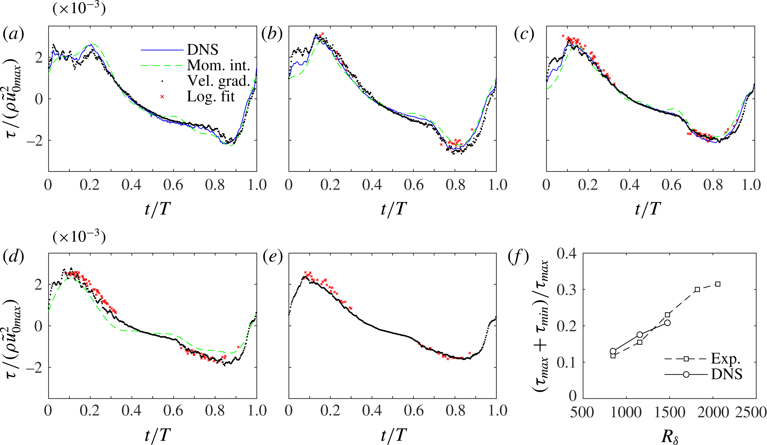
Figure 6 compares the wall shear stress obtained from the experimental data, using the three approaches, with the DNS-obtained wall shear stress. A reasonably good agreement between DNS and the velocity gradient method is generally observed, apart from early in the accelerating phase of the positive half-cycle, where the experimental shear stress shows a hump followed by high frequency fluctuations, which is most pronounced in figure 6(b,c). These deviations from the DNS are due to the large increase in pressure in the tunnel during the accelerating phase of the positive half-cycle, which causes a slight depression of the acrylic bed and outward deformation of the glass side walls, which in turn affects the refraction of the laser beams and results in a displacement of the LDA sampling volume to a higher position above the wall where velocity is larger. This results in the apparently higher shear stresses compared to the numerical simulations. In the negative half-cycle the differences between experiments and numerical simulations are smaller because the flow acceleration is much weaker compared to the positive half-cycle.
Equation (4.2) can only be applied when a logarithmic layer is present, therefore the logarithmic fit wall shear stress is only available during certain phases of the flow. Despite some scatter, the log-law results match with the DNS and velocity gradient results, and the agreement between the peak wall shear stresses is very good.
The momentum integral method applied to the experimental data shows reasonable agreement with the velocity gradient method and the DNS, as seen in figure 6(a–c). In order to limit the scatter in the shear stress from the numerical integration, equation (4.1) was applied to the smoothed velocities (by only considering the first six harmonics of the velocity), which inevitably causes some discrepancies with the other approaches as higher oscillations in the shear stress are also removed. In figure 6(d) for
 $R_{\unicode[STIX]{x1D6FF}}=1820$
, the comparison is only between the three methods applied to the experimental data. The agreement is fairly good apart from near
 $t/T\approx 0.3$
. For
 $R_{\unicode[STIX]{x1D6FF}}=2057$
the momentum integral method did not provide acceptable results, most probably because the propagation of numerical errors was too large due to the combination of a relatively coarse measurement resolution and very large velocity gradients.
Despite equal velocity maxima during both half-cycles, it is shown for all
 $R_{\unicode[STIX]{x1D6FF}}$
that the peak wall shear stress in the positive direction is higher compared to the negative direction. This results from the differences in flow acceleration between the two half-cycles, as shown previously (e.g. van der A et al.
Reference van der A, O’Donoghue, Davies and Ribberink2011; Yuan & Madsen Reference Yuan and Madsen2014; Scandura et al.
Reference Scandura, Faraci and Foti2016). In figure 6(f) the asymmetry in the wall shear stress, here defined as
 $(\unicode[STIX]{x1D70F}_{max}+\unicode[STIX]{x1D70F}_{min})/\unicode[STIX]{x1D70F}_{max}$
, is shown as a function of
 $R_{\unicode[STIX]{x1D6FF}}$
. The experimental results in figure 6(f) are from the velocity gradient method, since the shear stress could be obtained for all
 $R_{\unicode[STIX]{x1D6FF}}$
with this method. To obtain the maxima, the shear stress time series were first smoothed by taking only the first 10 harmonics, which made the asymmetry ratio less sensitive to high frequency fluctuations occurring around the maxima. The shear stress asymmetry increases with increasing
 $R_{\unicode[STIX]{x1D6FF}}$
and agreement between experiment and DNS is generally good. Based on DNS alone, Scandura et al. (Reference Scandura, Faraci and Foti2016) showed for asymmetric flows with the same
 $Asy$
that there is a local minimum in
 $(\unicode[STIX]{x1D70F}_{max}+\unicode[STIX]{x1D70F}_{min})/\unicode[STIX]{x1D70F}_{max}$
in the region
 $R_{\unicode[STIX]{x1D6FF}}=800-1100$
. Unfortunately the lack of experimental conditions in this region does not allow us to confirm or otherwise the existence of this minimum.
Generally, as Reynolds number increases the peak in wall shear stress in the positive half-cycle shifts to earlier phases in the cycle. During the negative half-cycle the peaks are less distinct due to the lower acceleration, but what can be best seen is the rapid increase in shear stress which, for example, for
 $R_{\unicode[STIX]{x1D6FF}}=846$
occurs at
 $t/T=0.8$
. As demonstrated later, this phase corresponds to the transition to turbulent flow and is seen to occur earlier in the cycle as
 $R_{\unicode[STIX]{x1D6FF}}$
increases.
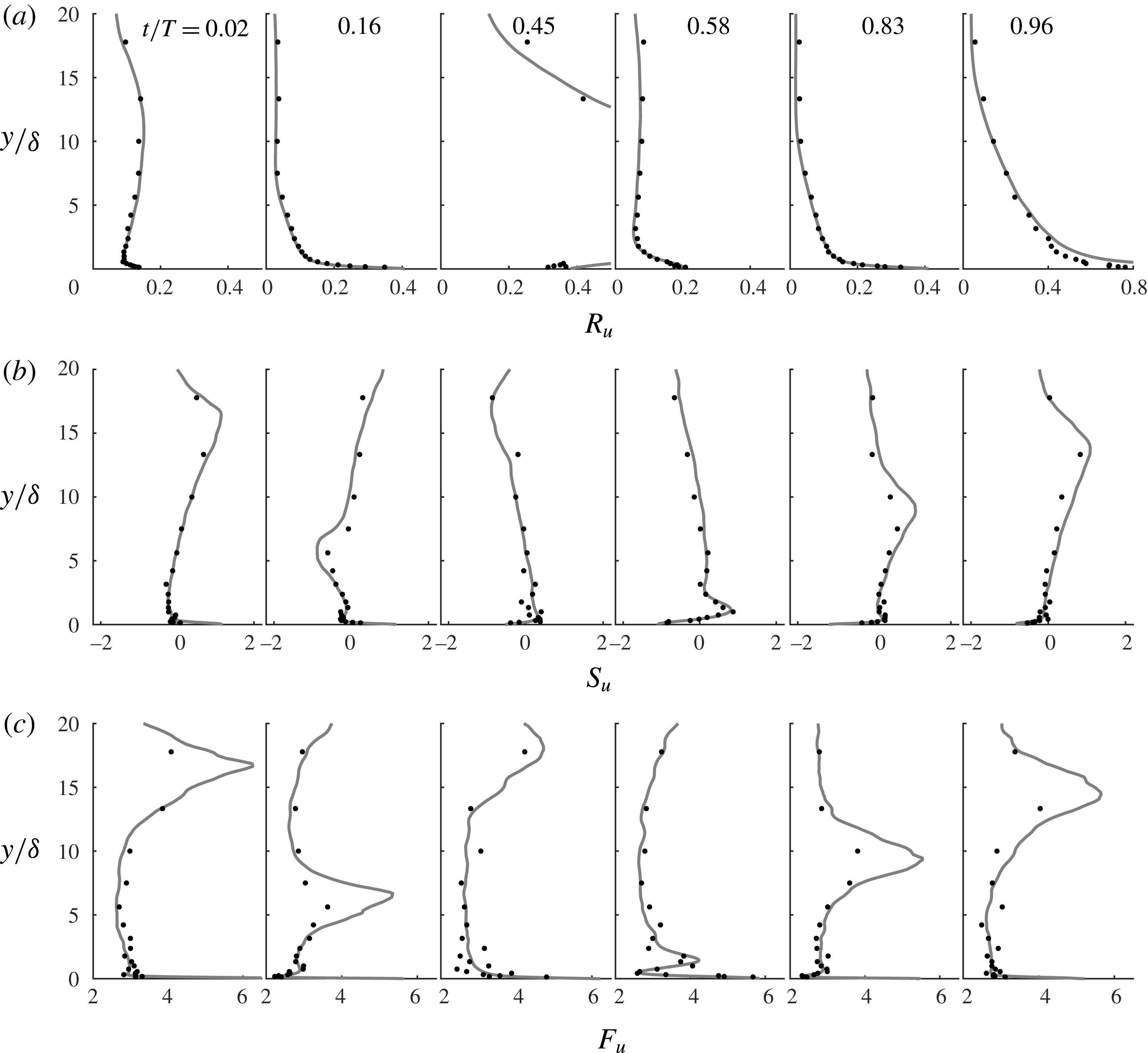
Vertical profiles of (a) streamwise turbulence intensity, (b) skewness and (c) flatness for
 $R_{\unicode[STIX]{x1D6FF}}=1155$
. Experiments (dots), DNS (lines).
4.3 Second-order and higher-order turbulence statistics
In figure 7 the experimental and numerical statistics of the streamwise velocity fluctuations are shown for six flow phases for
 $R_{\unicode[STIX]{x1D6FF}}=1155$
. In these figures, and throughout the remainder of this paper, we will use the variables
 $R_{u}=\langle {u^{\prime }}^{2}\rangle ^{1/2}/|\tilde{u} |$
,
 $S_{u}=\langle {u^{\prime }}^{3}\rangle /\langle {u^{\prime }}^{2}\rangle ^{3/2}$
and
 $F_{u}=\langle {u^{\prime }}^{4}\rangle /\langle {u^{\prime }}^{2}\rangle ^{2}$
to indicate the non-dimensional intensity, skewness and flatness of the streamwise velocity fluctuations. Similar notation applies to the statistics of the wall-normal,
 $v^{\prime }$
, and spanwise,
 $w^{\prime }$
, velocity fluctuations. Note that in the expressions for relative intensity,
 $R_{u}$
,
 $R_{v}$
and
 $R_{w}$
, the oscillatory component of the phase-averaged streamwise velocity
 $\tilde{u}$
is used in the denominator, instead of
 $\langle u\rangle$
, since the experimental and numerical phase-averaged velocities agreed only after subtraction of the time-averaged velocity,
 $\overline{u}$
(§ 4.1).
Figure 7 shows good agreement between the experimental and numerical results. Phases
 $t/T=0.16$
and 0.83 correspond to times when low-speed streaks have broken down. At these phases the turbulence statistics close to the wall are similar to those of steady turbulent channel flows (Scandura et al.
Reference Scandura, Faraci and Foti2016); in particular the relative intensity at the wall is close to 0.4. Several experimental studies involving steady turbulent boundary layers and channel flows report values close to 0.4 for the relative intensity of the streamwise wall shear stress (Barlow & Johnston Reference Barlow and Johnston1985; Alfredsson et al.
Reference Alfredsson, Johansson, Haritonidis and Eckelmann1988; Durst et al.
Reference Durst, Jovanovic and Sender1995). The results in figure 7 echo these findings because as
 $y/\unicode[STIX]{x1D6FF}$
tends to zero the streamwise relative intensity has the same statistics as the wall shear stress.
Figure 7 shows that in the
 $y$
direction the relative intensity is significant where the velocity gradient is high (see figures 4 and 5 for the velocity profiles), while intensity is very low at elevations corresponding to maximum streamwise velocity, where the velocity gradient vanishes. More specifically, at the phase of maximum free-stream velocity (
 $t/T=0.16$
), the relative intensity becomes very small at
 $y/\unicode[STIX]{x1D6FF}=5$
, which is the elevation at which the phase-averaged velocity is maximum. An analogous result occurs at the phase of minimum free-stream velocity (
 $t/T=0.83$
) in the negative half-cycle. However, because of the flow asymmetry, the elevation at which the relative intensity is very low shifts to a higher position compared to
 $t/T=0.16$
. At phases characterised by low streamwise velocity, such as
 $t/T=0.02$
,
 $R_{u}$
reaches a minimum at
 $y/\unicode[STIX]{x1D6FF}=1$
and then slightly increases up to
 $y/\unicode[STIX]{x1D6FF}=10$
, where the velocity has a minimum. At
 $t/T=0.45$
, the relative intensity tends to infinity because
 $\tilde{u}$
becomes zero at
 $y/\unicode[STIX]{x1D6FF}\approx 5$
.
Experimental and numerical skewness of streamwise velocity fluctuations,
 $S_{u}$
, show reasonably good agreement in figure 7. The largest discrepancies between experimental and numerical skewness are observed at
 $t/T=0.45$
, again due to low data rates at this phase because of the low streamwise velocity. Near the wall the skewness is mostly positive during the positive half-cycle and negative in the negative half-cycle. For example, the skewness profile at peak positive free-stream velocity (
 $t/T=0.16$
) is positive near the wall, decreases to a negative peak at
 $y/\unicode[STIX]{x1D6FF}\approx 5$
and increases for higher
 $y/\unicode[STIX]{x1D6FF}$
. The opposite behaviour is observed for the negative peak of the free-stream velocity (
 $t/T=0.83$
), but with the peak positive skewness occurring at higher
 $y/\unicode[STIX]{x1D6FF}$
because of the flow asymmetry.
Comparisons between experimental and numerical results for the flatness profiles of
 $u^{\prime }$
are shown in the third row of figure 7. Although agreement between experimental and numerical results is not as good as for skewness, the level of agreement is still sufficiently good to provide mutual validation of the experimental and numerical results. Generally, the flatness is greater than 4 at the wall but rapidly decreases with
 $y/\unicode[STIX]{x1D6FF}$
to values of 2–3 outside the viscous sublayer. Considering that a normal distribution has skewness equal to 0 and flatness equal to 3, the results show that the distribution of streamwise turbulent velocity fluctuations is far from normal, especially close to the wall.
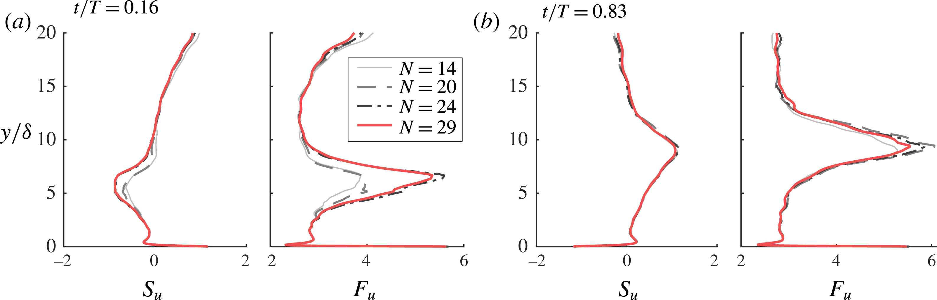
Effect of number of flow cycles on the DNS computed streamwise and skewness and flatness at phases of (a) maximum free-stream velocity and (b) minimum free-stream velocity.
 $R_{\unicode[STIX]{x1D6FF}}=1475$
.
Before discussing the next results for
 $R_{\unicode[STIX]{x1D6FF}}=1475$
, we will first demonstrate the convergence of the higher-order statistics in the DNS for this condition, which has the highest
 $R_{\unicode[STIX]{x1D6FF}}$
in the DNS and the shortest run duration (
 $N=29$
, cf. table 2). Figure 8 shows, for various
 $N$
, profiles of the streamwise skewness and flatness at maximum and minimum free-stream velocity, corresponding to phases of fully developed turbulence, when the spatial resolution requirements are maximum. Note that because of the spatial averaging over the horizontal
 $x{-}z$
plane, each additional flow cycle represents an increase of
 $n_{x}\times n_{z}$
samples used in the averaging procedure, i.e. for this Reynolds number there are 81 920 samples altogether. The close agreement between the results for
 $N=24$
and
 $N=29$
demonstrates that convergence is achieved in the DNS. The only slight discrepancy occurs at the maxima in the flatness profiles at higher elevations above the wall, which correspond to the elevations where the velocity gradient changes sign, which may be considered as the top of the boundary layer. At all other elevations, particularly closer to the wall, it is evident that convergence is achieved. Similar results were obtained for the wall-normal and spanwise velocity components, which are not shown here for brevity.
Vertical profiles of streamwise, wall-normal and spanwise (a) turbulence intensity, (b) skewness and (c) flatness for
 $R_{\unicode[STIX]{x1D6FF}}=1475$
.
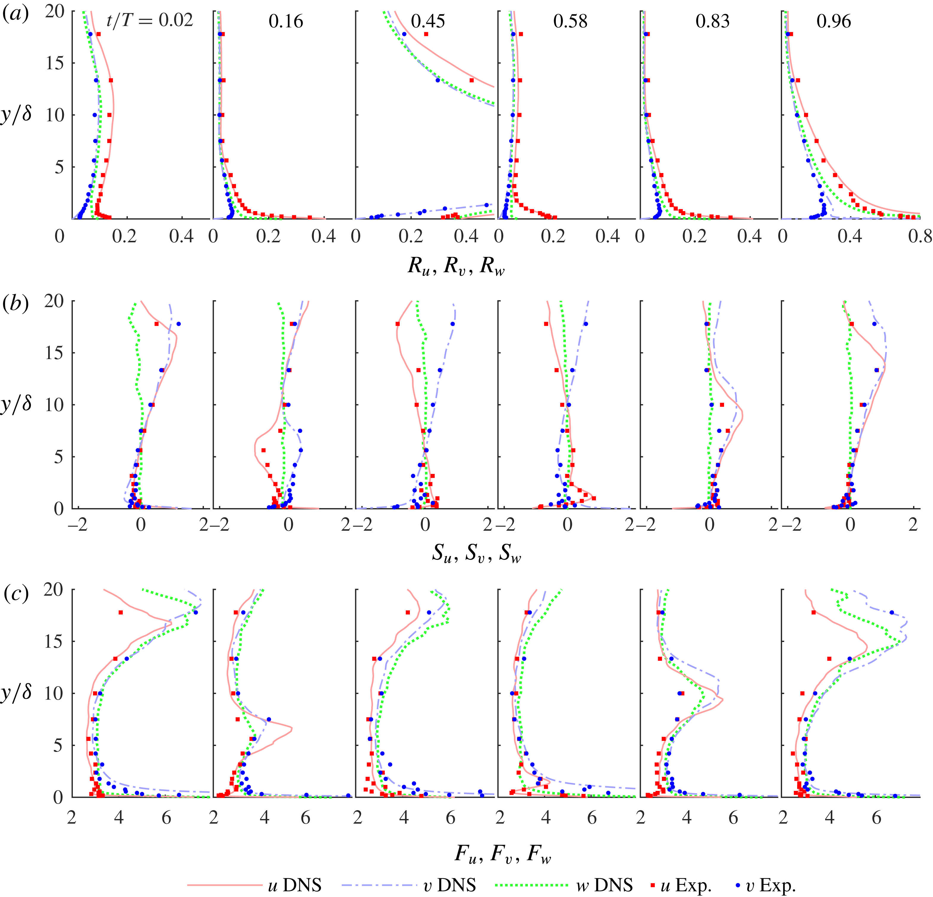
Figure 9 shows the velocity statistics for
 $R_{\unicode[STIX]{x1D6FF}}=1475$
, including the wall-normal and spanwise statistics. The streamwise statistics are very similar to the results shown for
 $R_{\unicode[STIX]{x1D6FF}}=1155$
, but agreement between the experiments and DNS is better because of lower scatter in the data due to higher LDA data sampling rates associated with the higher velocities. Wall-normal relative intensity,
 $R_{v}$
, is lower than
 $R_{u}$
, as expected for boundary layer flows, and, in contrast to
 $R_{u}$
,
 $R_{v}$
tends to zero as
 $y$
tends to zero. Early in the positive half-cycle the skewness of
 $v^{\prime }$
,
 $S_{v}$
, is positive near the wall; it then becomes negative as the flow accelerates and remains negative until late in the half-cycle. The same behaviour is observed in the negative half-cycle. The flatness of
 $v^{\prime }$
,
 $F_{v}$
, is very high close to the wall throughout the flow period, but rapidly decreases with distance from the wall.
The statistics of the spanwise velocity fluctuations shown in figure 9 are limited to the numerical results because spanwise velocity was not measured in the experiments. The profiles of
 $R_{w}$
are qualitatively similar to the profiles of
 $R_{u}$
, but quantitatively there are differences. In particular, at phases
 $t/T=0.16$
and 0.83,
 $R_{u}$
at the wall was approximately 0.4, while
 $R_{w}$
is approximately 0.25. We expect
 $S_{w}$
to be zero because in the spanwise direction negative fluctuations have the same probability of occurrence as positive fluctuations. Near the wall
 $S_{w}$
is indeed generally zero, but further away it deviates somewhat from zero, which is probably due to the finite size of the data sample. Far from the wall the trend of the flatness of
 $w^{\prime }$
,
 $F_{w}$
, is similar to
 $F_{v}$
, both qualitatively and quantitatively. However, very close to the wall
 $F_{v}$
is much higher than
 $F_{w}$
, which will be further illustrated in the following.
Experimental and numerical statistics of streamwise velocity and numerical statistics for the wall shear stress for
 $R_{\unicode[STIX]{x1D6FF}}=1475$
at
 $y=0.15$
mm (
 $y/\unicode[STIX]{x1D6FF}=0.1$
). (a) Phase-averaged velocity, (b) relative intensity, (c) skewness, (d) flatness.
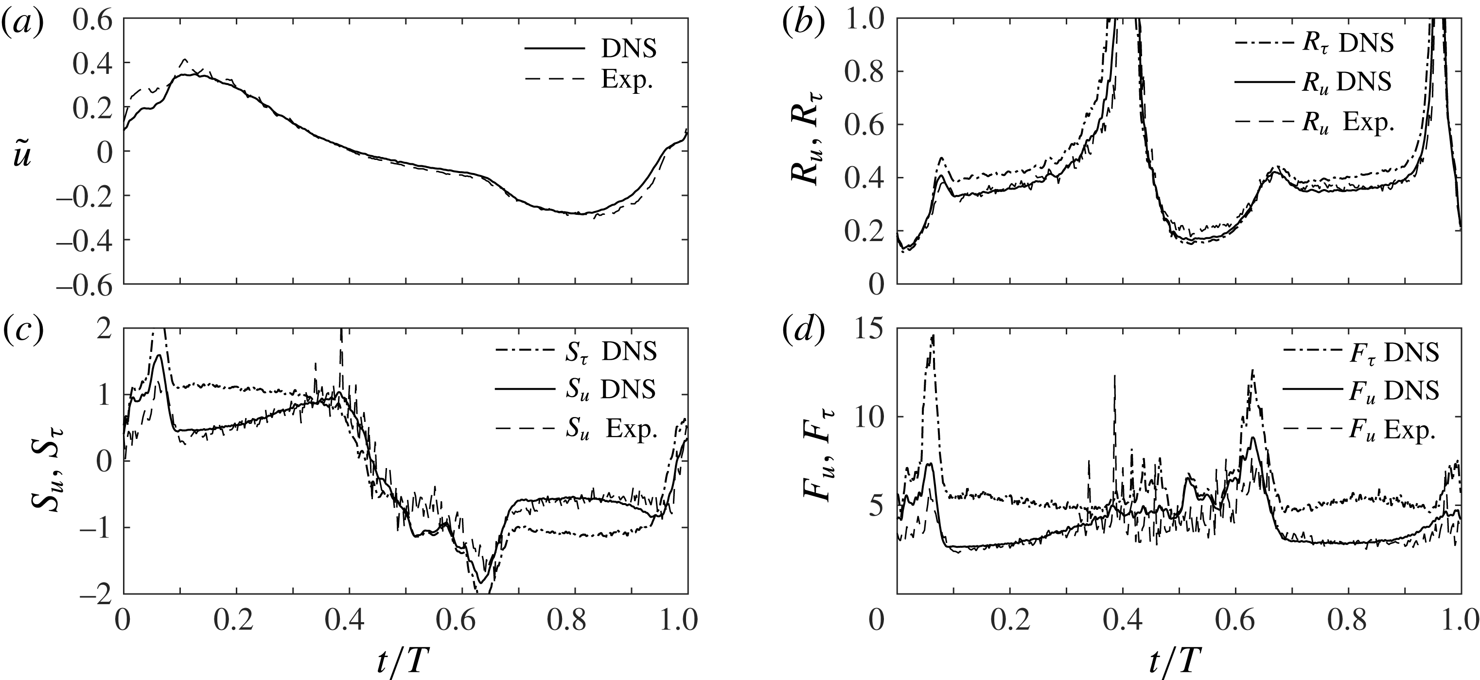
Figure 10 presents the experimental and numerical statistics of the streamwise velocity fluctuations at
 $y=0.15$
mm, together with the statistics of wall shear stress obtained numerically. Figure 10(a) shows good agreement between the experimental and numerical phase-averaged velocity, except for the hump at the beginning of the cycle, which is attributed to the pressure rise within the tunnel as explained in § 4.2. In figure 10(b) the relative intensities are in very good agreement, with no trace of a discrepancy at the beginning of the positive half-cycle as seen in the phase-averaged velocity. This is because the
 $y$
-gradient of the relative intensity is rather small close to the wall, whereas the gradient in
 $\tilde{u}$
is very large. The relative intensity of the wall shear stress fluctuations is seen to be slightly higher than the relative intensity of
 $u^{\prime }$
measured at
 $y=0.15$
mm. The skewness and the flatness, shown in figure 10(c,d) respectively, show good agreement between experiments and numerical simulations, except near flow reversal where the discrepancy can be largely attributed to the low LDA data rates.
In § 4.2 reliable estimates of the wall shear stress were obtained from velocity measurements at distances from the wall as large as
 $5\unicode[STIX]{x1D708}/u^{\ast }$
(
 ${\approx}y=0.15$
mm). However, figure 10(c,d) shows that this distance is too large to get reliable estimates of the higher-order statistics of the wall shear stress fluctuations, since
 $S_{\unicode[STIX]{x1D70F}}$
and
 $F_{\unicode[STIX]{x1D70F}}$
are much larger than
 $S_{u}$
and
 $F_{u}$
respectively.
Figure 10(c,d) shows very large peak values in the numerical higher-order wall shear stress statistics. The occurrence of such peaks was first observed by Scandura et al. (Reference Scandura, Faraci and Foti2016) in their DNS results for streamwise wall shear stress. Here, for the first time, we find experimental verification of these peaks: in figure 10(c,d) the statistics of streamwise velocity measured at
 $y=0.15$
mm show peaks at the same phases as the peaks in the wall shear stress.
Experimental and numerical streamwise and cross-stream velocity statistics for
 $R_{\unicode[STIX]{x1D6FF}}=1475$
at
 $y=3.56$
mm (
 $y/\unicode[STIX]{x1D6FF}=2.3$
). (a) Streamwise velocity, (b) relative intensity, (c) skewness, (d) flatness.
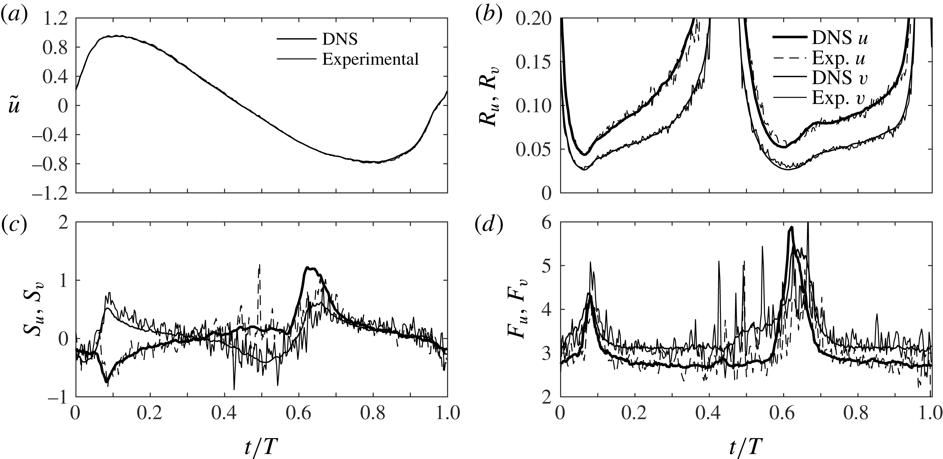
At larger distances from the wall, where the
 $y$
-gradient in velocity is less strong, the displacement of the LDA sampling volume due to the pressure rise has much smaller effect on the measured velocities. This can be seen in figure 11, where the statistics of the streamwise and wall-normal velocities at
 $y=3.56$
mm are presented, showing very good agreement between experiments and numerical simulations, both in terms of the streamwise
 $\tilde{u}$
and the relative intensities, including at phases early in the flow cycle.
Figure 12 shows the time-dependent streamwise, wall-normal and spanwise velocity statistics very near to the wall at
 $y=0.05$
mm for
 $R_{\unicode[STIX]{x1D6FF}}=1155$
. Only DNS data are shown because at positions this close to the wall experimental measurements are not available. It can be observed that from
 $t/T=0.02-0.08$
and from
 $t/T=0.60-0.65$
both the skewness and the flatness of all three velocity components have very large values. In particular, the flatness of the wall-normal velocities has values that are two orders of magnitude higher than those shown for
 $y=3.56$
mm in figure 11.
Figure 12 also shows that there is quite a large range of
 $t/T$
for which the higher-order statistics are approximately constant, with skewness having a value of approximately 1.1 for
 $u^{\prime }$
and the flatness being approximately 5.4 for
 $u^{\prime }$
, 25 for
 $v^{\prime }$
and 7 for
 $w^{\prime }$
.
DNS streamwise, wall-normal and spanwise velocity higher-order statistics very near to the wall for
 $R_{\unicode[STIX]{x1D6FF}}=1155~y=0.05$
mm
 $(y/\unicode[STIX]{x1D6FF}=0.03)$
. (a) Streamwise and spanwise velocity skewness, (b) streamwise and spanwise velocity flatness, (c) wall-normal velocity skewness, (d) wall-normal velocity flatness.

Phase of inception of the low-speed streaks breaking (
 $\unicode[STIX]{x1D719}_{1}$
) and phase at which the breaking process is completed (
 $\unicode[STIX]{x1D719}_{2}$
) as a function of the Reynolds number
 $R_{\unicode[STIX]{x1D6FF}}$
inferred from the measured time-dependent velocity statistics. (a) Positive half-cycle, (b) negative half-cycle.

Scandura et al. (Reference Scandura, Faraci and Foti2016) showed that close to the wall elongated low-speed streaks develop during the accelerating phase of the flow cycle and break into small turbulent structures before the free-stream velocity reaches its maximum value. The onset of breaking occurs at the moment of peak skewness (flatness),
 $t/T=\unicode[STIX]{x1D719}_{1}$
and ends when the skewness (flatness) has subsequently reduced to the plateau level at
 $t/T=\unicode[STIX]{x1D719}_{2}$
. This link between the dynamics of the near-wall turbulent structures and the velocity statistics also seems to hold for the present flows. Figure 13 presents the values of
 $\unicode[STIX]{x1D719}_{1}$
and
 $\unicode[STIX]{x1D719}_{2}$
determined from the experimental measurements at the lowest measurement point (
 $y=0.1$
mm); the values are plotted as a function of
 $R_{\unicode[STIX]{x1D6FF}}$
and separately for the positive and negative half-cycles. The values of
 $\unicode[STIX]{x1D719}_{1}$
and
 $\unicode[STIX]{x1D719}_{2}$
for the lowest three
 $R_{\unicode[STIX]{x1D6FF}}$
have been verified by the DNS. During phases before
 $\unicode[STIX]{x1D719}_{1}$
the flow is close to being laminar but contains low- and high-speed streaks that become stronger with time. Between
 $\unicode[STIX]{x1D719}_{1}$
and
 $\unicode[STIX]{x1D719}_{2}$
the low-speed streak breaking propagates in the fluid domain and at
 $\unicode[STIX]{x1D719}_{2}$
the flow enters the well-developed turbulence regime. One of the most apparent effects of the process of low-speed streaks breaking is the rapid increase in wall shear stress. As Reynolds number increases,
 $\unicode[STIX]{x1D719}_{1}$
and
 $\unicode[STIX]{x1D719}_{2}$
shift to earlier phases in the half-cycles. This trend is in agreement with Carstensen et al. (Reference Carstensen, Sumer and Fredsøe2010), who found the initiation of turbulent spots to happen earlier in the flow cycle with increasing Reynolds number. However, a direct comparison between phases we obtain here and those of Carstensen et al. (Reference Carstensen, Sumer and Fredsøe2010) is not possible since their study involved sinusoidal oscillatory motion. The gradient in the curves in figure 13 reduces with increasing
 $R_{\unicode[STIX]{x1D6FF}}$
, hence it is likely that even at very large Reynolds numbers there is still a range of phases after flow reversal when the flow is not in the regime of well-developed turbulence. Two distinct effects of the flow asymmetry are also noticeable in the results shown in figure 13. First, in the positive half-cycle
 $\unicode[STIX]{x1D719}_{1}$
and
 $\unicode[STIX]{x1D719}_{2}$
occur much sooner after flow reversal compared to the negative half-cycle. Second, for all
 $R_{\unicode[STIX]{x1D6FF}}$
, the phase difference
 $\unicode[STIX]{x1D719}_{2}-\unicode[STIX]{x1D719}_{1}$
is smaller during the onshore half-cycle compared to the offshore half-cycle, indicating that the breakup of low-speed streaks occurs more rapidly during the positive flow cycle.
A more comprehensive view of the distribution of skewness and flatness of the velocity fluctuations is provided by plotting these statistics in the phase-space plane, as shown in figure 14 for
 $R_{\unicode[STIX]{x1D6FF}}=1155$
. To better highlight the regions where a normal distribution can be detected, the quantity
 $F_{u}^{\prime }=F_{u}-3$
is shown, because a normal distribution has flatness equal to 3.
The black lines in figure 14 represent the elevation where
 $\unicode[STIX]{x2202}u/\unicode[STIX]{x2202}y=0$
, i.e. the elevation where the velocity gradient changes sign, which may also be seen as a proxy for the boundary layer thickness. It can be observed that both
 $S_{u}$
and
 $F_{u}^{\prime }$
have very low value along these lines. Generally,
 $|S_{u}|$
is rather small above the
 $\unicode[STIX]{x2202}u/\unicode[STIX]{x2202}y=0$
line and reaches very large values well below the line. Similar features can be observed for
 $F_{u}^{\prime }$
in figure 14(b). Figure 14(b) also shows that appreciable negative values of
 $F_{u}^{\prime }$
occur in a small area around
 $y/\unicode[STIX]{x1D6FF}=0.3$
. Therefore, the flatness has mostly larger values compared to a normal distribution. Based on these results, a normal distribution for the streamwise velocity fluctuations may be expected in the area that extends above the
 $\unicode[STIX]{x2202}u/\unicode[STIX]{x2202}y=0$
line for the half-cycle, where both
 $S_{u}$
and
 $F_{u}^{\prime }$
have low values.
Time–space distribution of streamwise (a) skewness
 $S_{u}$
and (b) flatness
 $F_{u}^{\prime }$
for
 $R_{\unicode[STIX]{x1D6FF}}=1155$
. DNS data.
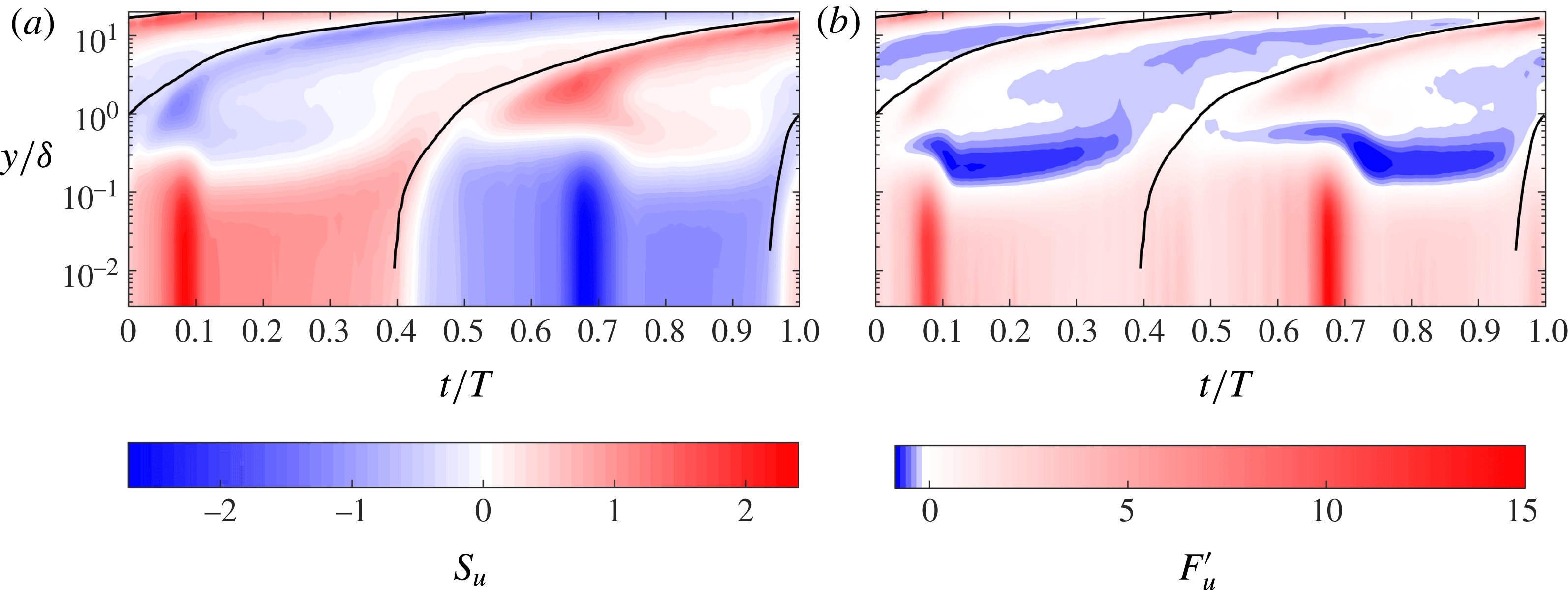
Close to the wall the sign of
 $S_{u}$
remains unaltered during each half-cycle while the sign of
 $F_{u}^{\prime }$
remains unaltered during the entire flow cycle. Both
 $S_{u}$
and
 $F_{u}^{\prime }$
show very large values close to the wall at the phase
 $\unicode[STIX]{x1D719}_{1}\approx 0.09$
(see figure 13), when breaking of the low-speed streaks starts. This is in agreement with the results shown in figure 12, but in the phase-space results shown in figure 14 it can be seen that these large values extend up to
 $y/\unicode[STIX]{x1D6FF}=0.2$
, corresponding approximately to the beginning of the logarithmic region.
It is not straightforward to explain why the skewness is positive or negative at every location in the phase-space plane, but we can provide a qualitative explanation why the skewness of
 $u^{\prime }$
close to the wall is positive during the positive half-cycle. For a location
 $y=y_{p}$
close to the wall, the flow occurring during the positive half-cycle at locations
 $y>y_{p}$
is characterised by streamwise velocities that are much higher than those at elevations
 $y<y_{p}$
. Therefore, fluid particles from
 $y>y_{p}$
cause a positive
 $u^{\prime }$
fluctuation of greater magnitude than the negative fluctuation caused by particles coming from
 $y<y_{p}$
. As a result, the third-order moment of
 $u^{\prime }$
is greater than zero and
 $S_{u}>0$
. The opposite occurs during the negative half-cycle.
Trend of the flatness as a function of the skewness for
 $R_{\unicode[STIX]{x1D6FF}}=1155$
based on all the DNS data in the fluid domain. (a) Streamwise velocity fluctuations: solid line,
 $F_{u}=2+0.15S_{u}+1.56S_{u}^{2}$
; dashed line,
 $F_{u}=2.65+1.62S_{u}^{2}$
. (b) Wall-normal velocity fluctuations: solid line,
 $F_{v}=2.62-0.88S_{v}+4.39S_{v}^{2}$
; dashed line,
 $F_{v}=3.13+2.48S_{v}^{2}$
.

The
 $S_{u}$
and
 $F_{u}^{\prime }$
distributions seen in figure 14 suggest that an interrelation exists between the two statistics. This possibility is explored in figure 15, where
 $F_{u}$
and
 $F_{v}$
are plotted as a function of their skewness. For the streamwise velocity most of the data fall within a band adjacent to the parabola given by the equation
 $F_{u}=2+0.15S_{u}+1.56S_{u}^{2}$
, indicated by the continuous line in figure 15(a). The minimum flatness occurs for
 $S_{u}=0$
and is approximately 2.2. For
 $S_{u}=0$
the flatness does not exceed values of about 6. These values mainly occur near flow reversal when the skewness is small but the flatness can be large. Generally, large values of flatness involve high values of skewness. A similar behaviour is observed for the wall-normal velocity component shown in figure 15(b) where the data mostly fall above the parabola described by the equation
 $F_{v}=2.62-0.88S_{v}+4.39S_{v}^{2}$
. The asymmetry in the distribution of the data with respect to
 $S_{v}=0$
is due to
 $S_{v}$
being negative for most of the flow cycle as shown in figure 12(c) for a point near the wall. The minimum value for
 $F_{v}$
is about 2.75 and occurs when
 $S_{v}$
is approximately zero. These findings are similar to those reported by Jovanovic, Durst & Johansson (Reference Jovanovic, Durst and Johansson1993), who analysed skewness and flatness measured from various steady-flow boundary layer experiments and found that
 $F$
and
 $S$
are correlated by
 $F_{u}=2.65+1.62S_{u}^{2}$
and
 $F_{v}=3.13+2.48S_{v}^{2}$
. In figure 15(a) there is a reasonably good agreement between the present results and Jovanovic et al. (Reference Jovanovic, Durst and Johansson1993), while in figure 15(b) there is agreement for low skewness values only.
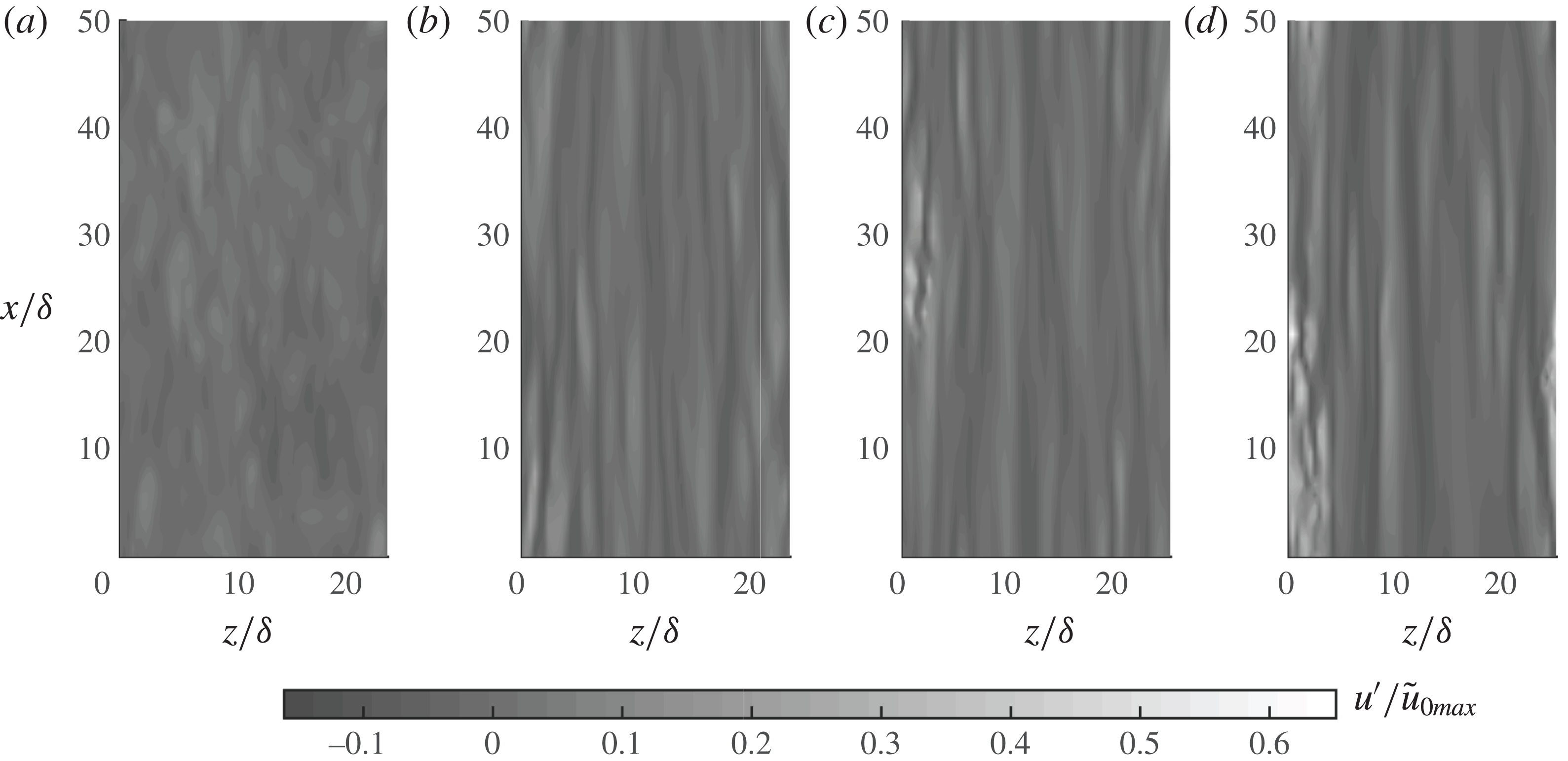
Contour plot in grey-scale of the streamwise velocity fluctuation
 $u^{\prime }$
at
 $y/\unicode[STIX]{x1D6FF}=0.16$
:
 $R_{\unicode[STIX]{x1D6FF}}=1155$
; (a)
 $t/T=0.013$
, (b)
 $t/T=0.052$
, (c)
 $t/T=0.063$
, (d)
 $t/T=0.077$
.
A possible explanation for the discrepancy between the present results and Jovanovic et al. (Reference Jovanovic, Durst and Johansson1993), besides the fact that the present result is for oscillatory flow while Jovanovic et al. result is for steady flow, is that the high values of
 $F_{v}$
obtained from DNS very close to the wall are very difficult to measure experimentally. For example, the LDA measurements of Durst et al. (Reference Durst, Jovanovic and Sender1995), in the near-wall region of a turbulent pipe flow, show that as
 $y^{+}$
decreases
 $F_{v}$
attains a maximum value of 5.25 at
 $y^{+}\approx 12$
and then decreases to zero; the LDA measurements of Karlsson & Johansson (Reference Karlsson, Johansson and Adrian1986) for a closed channel flow show that as
 $y^{+}$
decreases
 $F_{v}$
attains a maximum value of about 8 and, similar to Durst et al. (Reference Durst, Jovanovic and Sender1995), decreases to zero closer to the wall. The maximum
 $F_{v}$
used by Jovanovic et al. (Reference Jovanovic, Durst and Johansson1993) to determine the correlation between
 $F_{v}$
and
 $S_{v}$
shown in figure 15(b) is equal to 8, whereas the numerical results presented here show that much higher values occur very close to the wall.
4.4 The origin of high flatness in velocity fluctuations near the wall
Figure 12 has shown that the higher-order statistics of the velocity fluctuations close to the wall can be very large. In particular,
 $F_{v}$
takes values of several hundred. An explanation for why this occurs is given in the following.
Figure 16 shows the fluctuation of streamwise velocity in the plane
 $y/\unicode[STIX]{x1D6FF}=0.16$
for
 $R_{\unicode[STIX]{x1D6FF}}=1155$
, for the range of phases in which the flatness and the skewness increase rapidly and reach very large values. For
 $t/T=0.013$
there is no sign of large-scale spatial organisation of the velocity fluctuation. Between
 $t/T=0.013-0.063$
, elongated low-speed streaks emerge and grow stronger. By
 $t/T=0.063$
streak breaking has started in areas where high positive velocity fluctuations appear and these so-called ‘turbulent spots’ spread in the fluid domain with increasing flow as can be seen by
 $t/T=0.077$
.
Figure 17 shows the wall-normal velocity fluctuations in the plane
 $y/\unicode[STIX]{x1D6FF}=0.16$
for the same phases as in figure 16. Figure 17(a) is similar to figure 16(a) in that the
 $v^{\prime }$
fluctuations are essentially randomly distributed. By
 $t/T=0.052$
the
 $v^{\prime }$
fluctuations are organised in elongated streaks, similar to figure 16(b). However, unlike figure 16(b), the streaks are very narrow and there are large areas where
 $v^{\prime }$
is close to zero. In figure 17(c,d), low
 $v^{\prime }$
fluctuations still occupy most of the surface, but small isolated areas of high
 $v^{\prime }$
have appeared.
In order to illustrate quantitatively how this distribution of the velocity fluctuation affects the statistics, we write the flatness of
 $v$
as
 $\widehat{q^{2}}/\widehat{q}^{2}$
, where
 $q=v^{\prime 2}$
and the hat symbol denotes an average over the
 $x$
-
 $z$
plane. When we calculate the terms in the numerator and denominator with reference to figure 17(d), we obtain
 $\widehat{q^{2}}=7.95\times 10^{-8}$
and
 $\widehat{q}=2.32\times 10^{-5}$
respectively. We note that in figure 17(d)
 $q$
is larger than
 $\widehat{q}$
within a small surface that is 7.37 % of the total surface. When we now set all the values outside this small portion of the bottom boundary to zero, the result is
 $\widehat{q^{2}}=7.94\times 10^{-8}$
and
 $\widehat{q}=2.19\times 10^{-5}$
, which are very close to the previous values. This shows that almost all the significant values of
 $q$
are concentrated within a small area. Consequently,
 $\widehat{q}$
is small and large fluctuations in
 $q$
given by
 $q^{\prime }=q-\widehat{q}$
are only present within the small area. Remembering that
 $\widehat{q^{2}}=\widehat{q}^{2}+\widehat{q^{\prime 2}}$
and considering that the fluctuation
 $q^{\prime }$
is large, it emerges that
 $\widehat{q^{2}}$
is significantly larger than
 $\widehat{q}^{2}$
, therefore the flatness
 $F=\widehat{q^{2}}/\widehat{q}^{2}$
attains large values.
Contour plot in grey-scale of the wall-normal velocity fluctuation
 $v^{\prime }$
at
 $y/\unicode[STIX]{x1D6FF}=0.16$
:
 $R_{\unicode[STIX]{x1D6FF}}=1155$
; (a)
 $t/T=0.013$
, (b)
 $t/T=0.052$
, (c)
 $t/T=0.063$
, (d)
 $t/T=0.077$
.
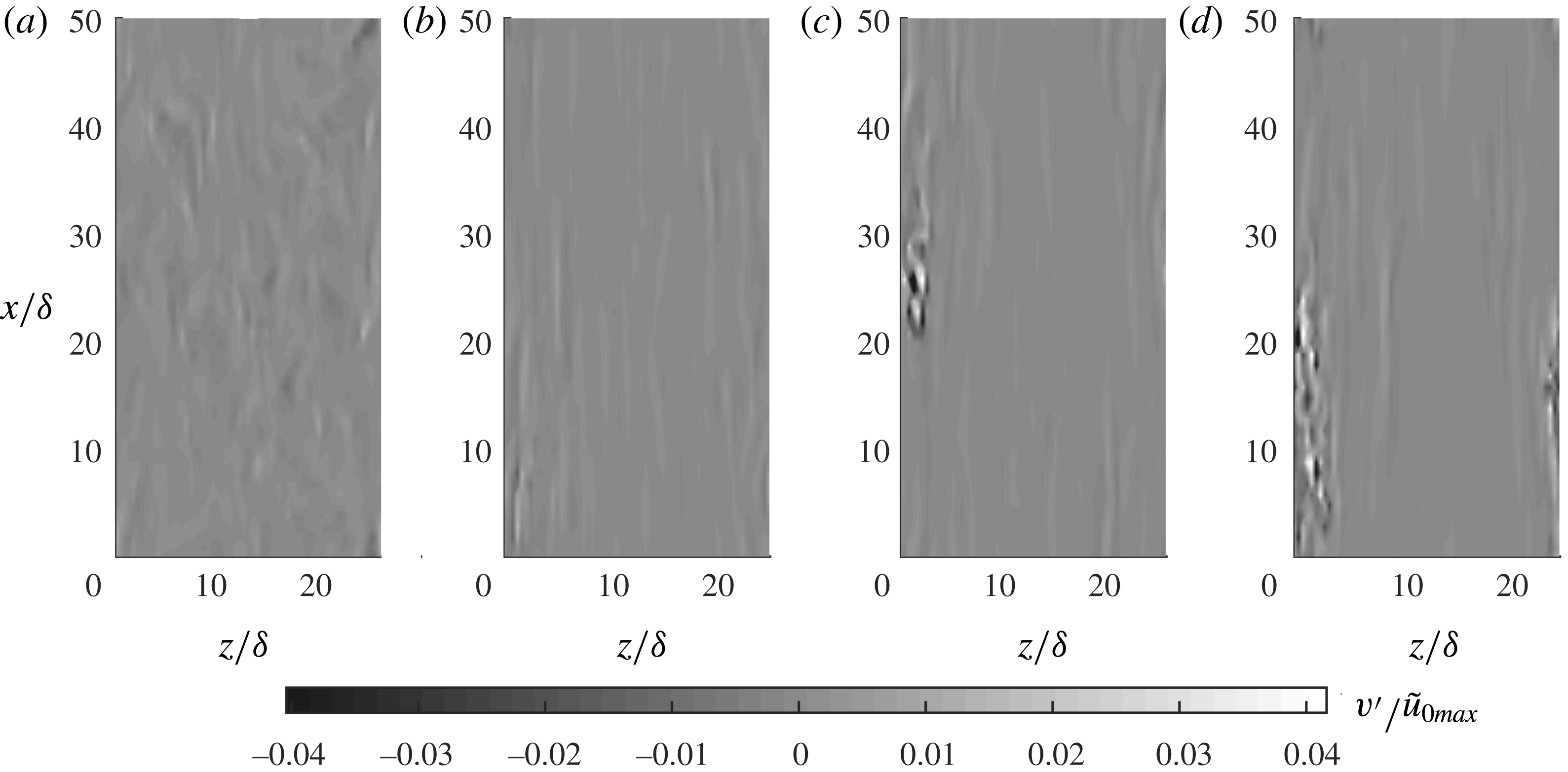
The reason for the large flatness is therefore due to spatial intermittency, i.e. to localised large velocity fluctuations separated by large areas where the velocity fluctuations are small. The flatness can therefore be used as a measure of intermittency (Tsinober Reference Tsinober2009). In particular, the inverse of the flatness provides a measure of the fraction of area where the variable is significant. The latter agrees with the earlier observation that, after the onset of breaking of the low-speed streaks, the flatness decreases, as large fluctuations become less localised in space. It is worthwhile noting that in the present case spatial intermittency also involves temporal intermittency. A probe positioned at a fixed location, such as the LDA sampling volume, measures velocity fluctuations of large magnitude during short time intervals, which are separated by long time intervals of low-magnitude velocity fluctuations. This is one of the reasons why it is difficult for the LDA to obtain sufficient data to properly resolve the higher-order statistics. This is less of an issue for the DNS simulations because of the possibility of applying spatial averaging in addition to temporal (or phase) averaging.
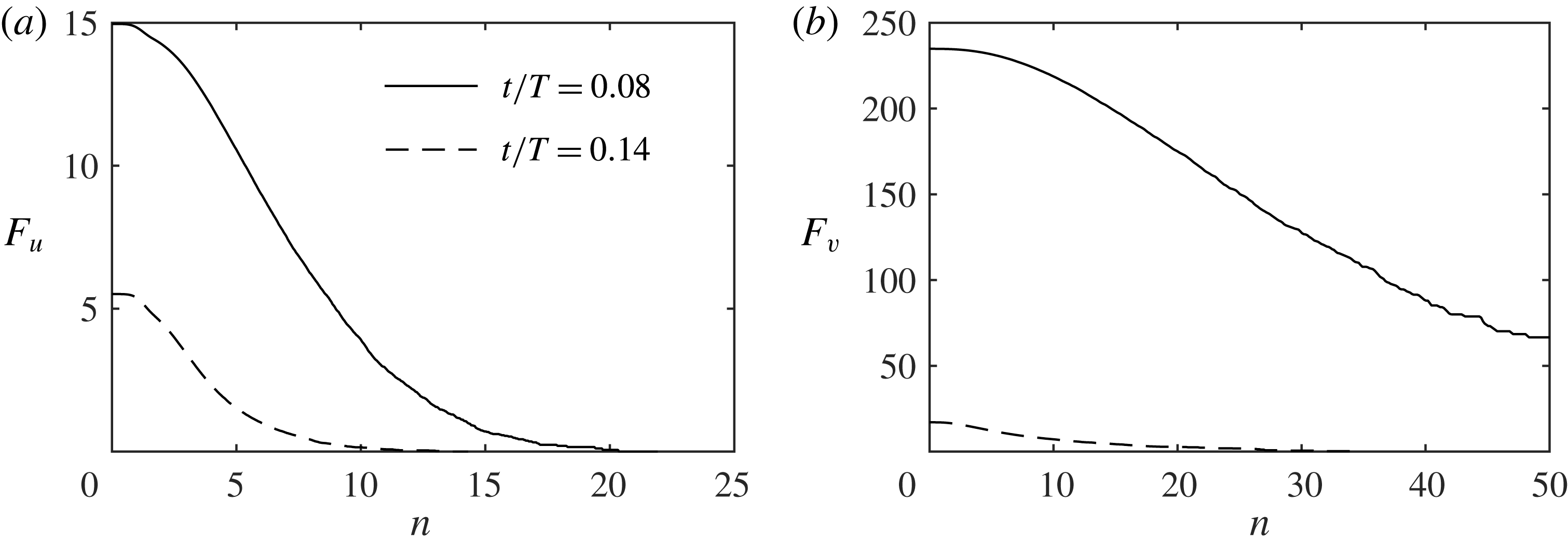
How the flatness is affected by the largest velocity fluctuations can be further appreciated through figure 18, which shows
 $F_{u}$
and
 $F_{v}$
calculated by considering only data that exceed
 $n$
times the root-mean-square (r.m.s.) of the velocity fluctuations; the calculation is done for varying
 $n$
. Figure 18(a,b) shows
 $F_{u}$
and
 $F_{v}$
respectively at two phases; the first corresponds to the phase of figure 17(d), when elongated low-speed streaks are still present in the domain; the second corresponds to a later phase when low-speed streaks are broken in the entire fluid domain. Figure 18(b) shows that as
 $n$
increases
 $F_{v}$
at
 $t/T=0.08$
undergoes only a small percentage reduction with respect to
 $n=0$
. For example, for
 $n=15$
the flatness of
 $v$
is about 90 % of the true value. Although to a lesser extent, a similar feature is observed for
 $F_{u}$
shown in figure 18(a), where for
 $n=5$
the flatness is approximately 70 % of the true value. After low-speed streak breaking has occurred (
 $t/T=0.14$
), the velocity fluctuations occur more uniformly in space, causing a decrease in the flatness. Indeed, in figure 18(a,b) the flatness for
 $n=5$
and
 $n=15$
respectively is small.
 $F_{v}$
takes a value of approximately 17 close to the wall, which is still relatively large, indicating that intermittency in the wall-normal velocity is still significant very close to the wall, even after transition to turbulence.
Flatness of velocity fluctuations (a)
 $u^{\prime }$
and (b)
 $v^{\prime }$
for
 $R_{\unicode[STIX]{x1D6FF}}=1155$
at
 $y/\unicode[STIX]{x1D6FF}=0.03$
computed by excluding the values of the velocity fluctuations that have lower magnitude than
 $n$
times the r.m.s. of the velocity fluctuations. The variable
 $n$
is shown along the
 $x$
-axis.
4.5 Probability density functions of velocity fluctuations
In the previous section the higher-order statistics of the velocity fluctuations provided information on the shape of the probability density functions (pdf) of the velocity fluctuations and indicated the regions of the flow field where a normal distribution is expected. In this section, the analysis is extended by focusing directly on the pdfs. In general, knowledge of the pdfs of the velocity fluctuations is important for the formulation of theoretical models of incipient motion of sediments based on probabilistic approaches and to predict diffusion processes in fluids (Wu & Yang Reference Wu and Yang2004). To determine, for example, the pdf of the streamwise velocity
 $u$
, the velocity fluctuations
 $u^{\prime }$
in a given
 $x{-}z$
plane at a given phase were determined for all flow cycles. The range between the minimum and the maximum of
 $u^{\prime }$
was divided into
 $M\unicode[STIX]{x0394}u^{\prime }$
intervals with a variable width: they are narrower near
 $u^{\prime }=0$
, where most data occur, and they grow in width towards the extremes of
 $u^{\prime }$
, where data are more sparse. For each interval the value of the pdf was determined from
 $pdf=m/(M\unicode[STIX]{x0394}u^{\prime })$
, where
 $m$
is the number of data samples falling in the interval
 $\unicode[STIX]{x0394}u^{\prime }$
. The value of
 $M$
was fixed to 180 which allowed a sufficient amount of data in each interval, and at the same time an adequate resolution of the pdfs. The wall-normal and spanwise pdfs were similarly determined. Figure 19 shows the pdf of
 $u^{\prime }$
at sixteen phases of the flow cycle and at four different elevations. The first two elevations are located close to the wall, where the skewness shows large
 $y$
-gradients (see figure 14); the other two elevations are located further away from the wall, where the streamwise velocity follows a log-law profile when turbulence is well developed.
Probability density of
 $u^{\prime }$
for
 $R_{\unicode[STIX]{x1D6FF}}=1155$
.
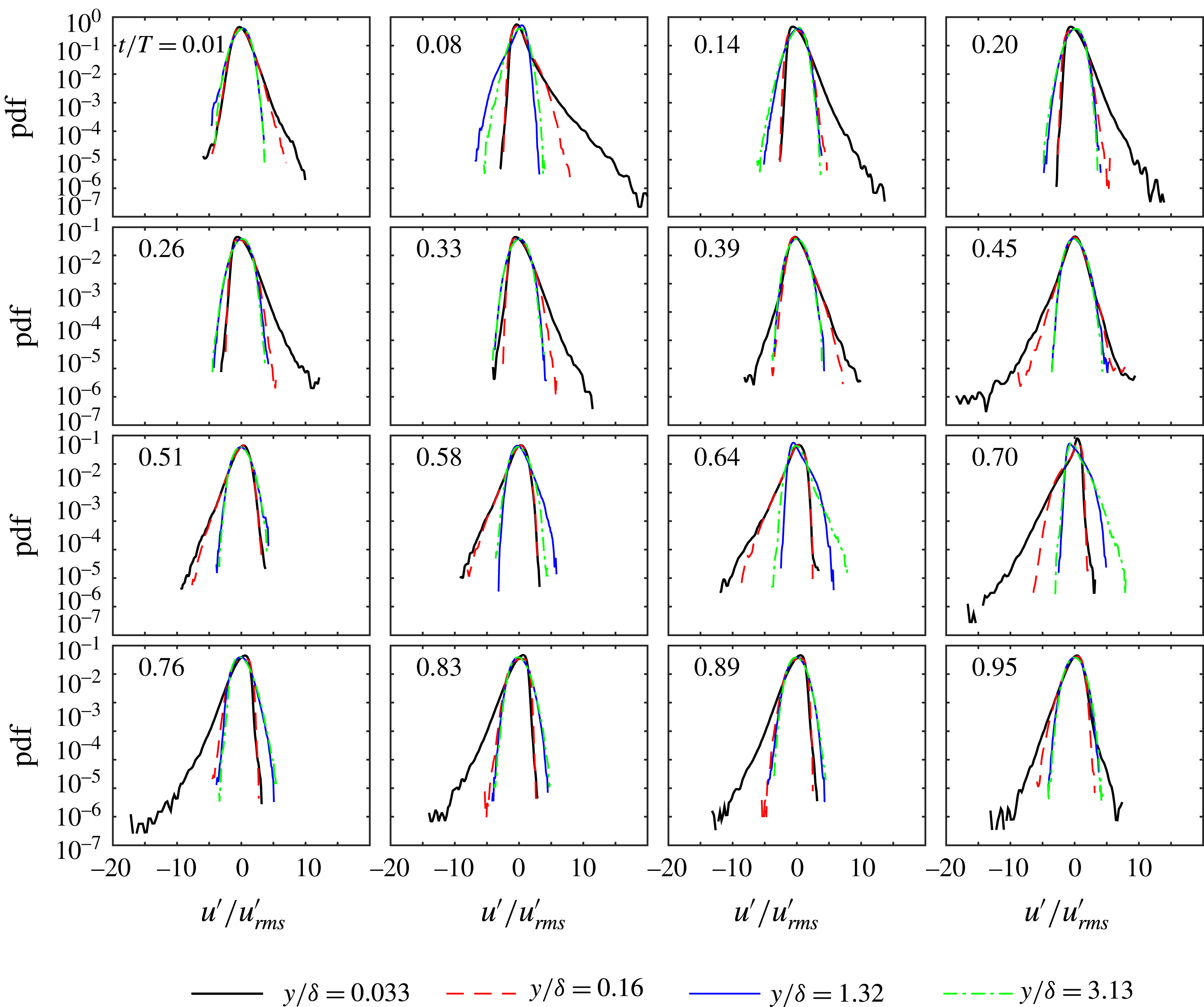
Probability density of
 $v^{\prime }$
for
 $R_{\unicode[STIX]{x1D6FF}}=1155$
.

The pdfs are shown as semilog graphs to show the large velocity fluctuations occurring with low values of probability density. The main observations from figure 19 can be summarised as follows.
(i) The pdfs show long tails close to the wall, especially in the pre-turbulent stage of each half-cycle (
 $0<t/T<0.14$
and
$0.58<t/T<0.76$
); this result is consistent with the large flatness seen at these phases.
(ii) During the positive (negative) half-cycle the positive (negative) fluctuations decrease significantly as
$y/\unicode[STIX]{x1D6FF}$
increases, while the negative (positive) fluctuations are approximately constant.(iii) The previous point suggests that the large gradient in the statistics near
$y/\unicode[STIX]{x1D6FF}=0$
(seen in figure 14) is almost exclusively due to variations in the positive (negative) velocity fluctuations.(iv) Far from the wall (
$y/\unicode[STIX]{x1D6FF}=1.32{-}3.13$
), the pdfs show some variation with
$y/\unicode[STIX]{x1D6FF}$
prior to the transition to turbulence (
$0<t/T<0.14$
and
$0.58<t/T<0.76$
); during the remainder of the flow cycle the pdfs do not show any
$y/\unicode[STIX]{x1D6FF}$
dependency and are therefore very similar to each other.






Figure 20 shows the probability density function for
 $v^{\prime }$
for the same elevations considered in figure 19. The main observations are as follows.
(i) At each phase the pdfs show sharp peaks at
$v^{\prime }/v_{rms}^{\prime }=0$
because most values are close to zero and show long tails due to the few extremely large values of
$v^{\prime }$
in the distribution. This characteristic is especially noticeable close to the wall prior to the transition to turbulence and is responsible for the large flatness at these phases previously discussed.(ii) With the exception of phases near flow reversal (
$t/T=0.01$
,
$t/T=0.64$
), negative velocity fluctuations reach larger values than positive fluctuations, resulting in a slightly negative skewness (as seen previously in figure 12).(iii) At large distances from the wall (
$y/\unicode[STIX]{x1D6FF}=1.32$
and 3.13), the dimensionless fluctuations are limited to values less than 10; also, there are phase intervals (
$t/T=0.14$
–0.38; 0.70–0.95) when the pdfs at
$y/\unicode[STIX]{x1D6FF}=1.32$
and 3.13 are very close to each other and very similar to the corresponding pdfs of streamwise fluctuations.


For the spanwise velocity fluctuations, as already noted in figure 9, the pdfs (not shown) are characterised by a vanishing skewness, but are otherwise similar to the pdfs of
 $v^{\prime }$
.
From the foregoing it is clear that the pdfs generally depend on distance from the wall and on the flow phase. However, at a sufficient distance from the wall, and during phases characterised by well-developed turbulence, the pdfs do not show significant differences.
For use of pdfs in the formulation of probabilistic models of, for example, sediment transport, it is interesting to consider if probability density functions from the literature suitably describe the pdfs of velocity fluctuations reported here. It has been noted that the pdf of
 $u^{\prime }$
is approximately described by a log-normal distribution during the majority of the flow cycle. The equation for this distribution is reported in Scandura et al. (Reference Scandura, Faraci and Foti2016) amongst others, where the log-normal distribution was fitted to the frequency distribution of streamwise wall shear stress fluctuations obtained from DNS. The pdfs of
 $v^{\prime }$
shown here can be approximately described by a Pearson type IV distribution given by
 $$\begin{eqnarray}pdf=\frac{1}{b\unicode[STIX]{x1D6FD}(s-0.5,0.5)}\frac{|\unicode[STIX]{x1D6E4}(s+\text{i}\unicode[STIX]{x1D709}/2)|^{2}}{\unicode[STIX]{x1D6E4}(s)^{2}}\left[1+\left(\frac{v^{\prime }-\unicode[STIX]{x1D706}}{b}\right)^{2}\right]^{-s}\exp \left[-\unicode[STIX]{x1D709}\tan ^{-1}\left(\frac{v^{\prime }-\unicode[STIX]{x1D706}}{b}\right)\right],\end{eqnarray}$$
where
 $s$
,
 $\unicode[STIX]{x1D706}$
,
 $\unicode[STIX]{x1D709}$
and
 $b$
are the parameters of the distribution,
 $\unicode[STIX]{x1D6E4}$
is the gamma function,
 $\unicode[STIX]{x1D6FD}$
is the beta function and
 $\text{i}$
is the imaginary unit. Finally, the frequency distribution of
 $w^{\prime }$
are well described by the Pearson type VII distribution, previously used by Scandura et al. (Reference Scandura, Faraci and Foti2016) to fit the frequency distribution of spanwise wall shear stress.
Comparisons of the standard probability distributions and the distributions obtained from the numerical simulation data are shown in figure 21 for
 $R_{\unicode[STIX]{x1D6FF}}=1155$
and at
 $t/T=0.08$
. This phase has been selected because the velocity fluctuations exhibit large flatness and long tails at this phase and so the frequency distributions deviate strongly from a normal distribution. The comparisons in figure 21 are made for four elevations from the wall. Figure 21(a–d) show that the log-normal distribution describes the distribution of
 $u^{\prime }/u_{rms}^{\prime }$
rather well, except for large values of the fluctuation. Nevertheless, for values of the pdf larger than
 $10^{-2}$
the log-normal distribution provides a good description of the numerical data.
Figure 21(e–h) compares the probability distributions of
 $v^{\prime }/v_{rms}^{\prime }$
obtained from the numerical data with a Pearson type IV distribution. The type IV distribution describes the data well, again with the exception of very large
 $v^{\prime }/v_{rms}^{\prime }$
. Finally, figure 21(i–l) shows the comparison between the distribution
 $w^{\prime }/w_{rms}^{\prime }$
and the Pearson type VII distribution. The agreement between the numerical data and the theoretical distribution is reasonably good, both for large and small values of
 $w^{\prime }/w_{rms}^{\prime }$
. The fourth-order Gram–Charlier series distribution (Johnson, Kotz & Balakrishnan Reference Johnson, Kotz and Balakrishnan1994) was also tested against the numerical data, but provided good results only for elevations far from the wall where the flatness is not much larger than 3. This result is expected as the Gram–Charlier series is a truncated series expansion based on the normal distribution and is therefore suitable for distributions characterised by skewness and flatness not much larger than 0 and 3 respectively.
Comparison between the probability density computed by numerical simulation (dashed lines) and that provided by known theoretical distributions (continuous lines). (a–d) Streamwise velocity, log-normal distribution; (e–h) wall-normal velocity, Pearson type IV distribution; (i–l) spanwise velocity, Pearson type VII distribution;
 $t/T=0.08$
,
 $R_{\unicode[STIX]{x1D6FF}}=1155$
.
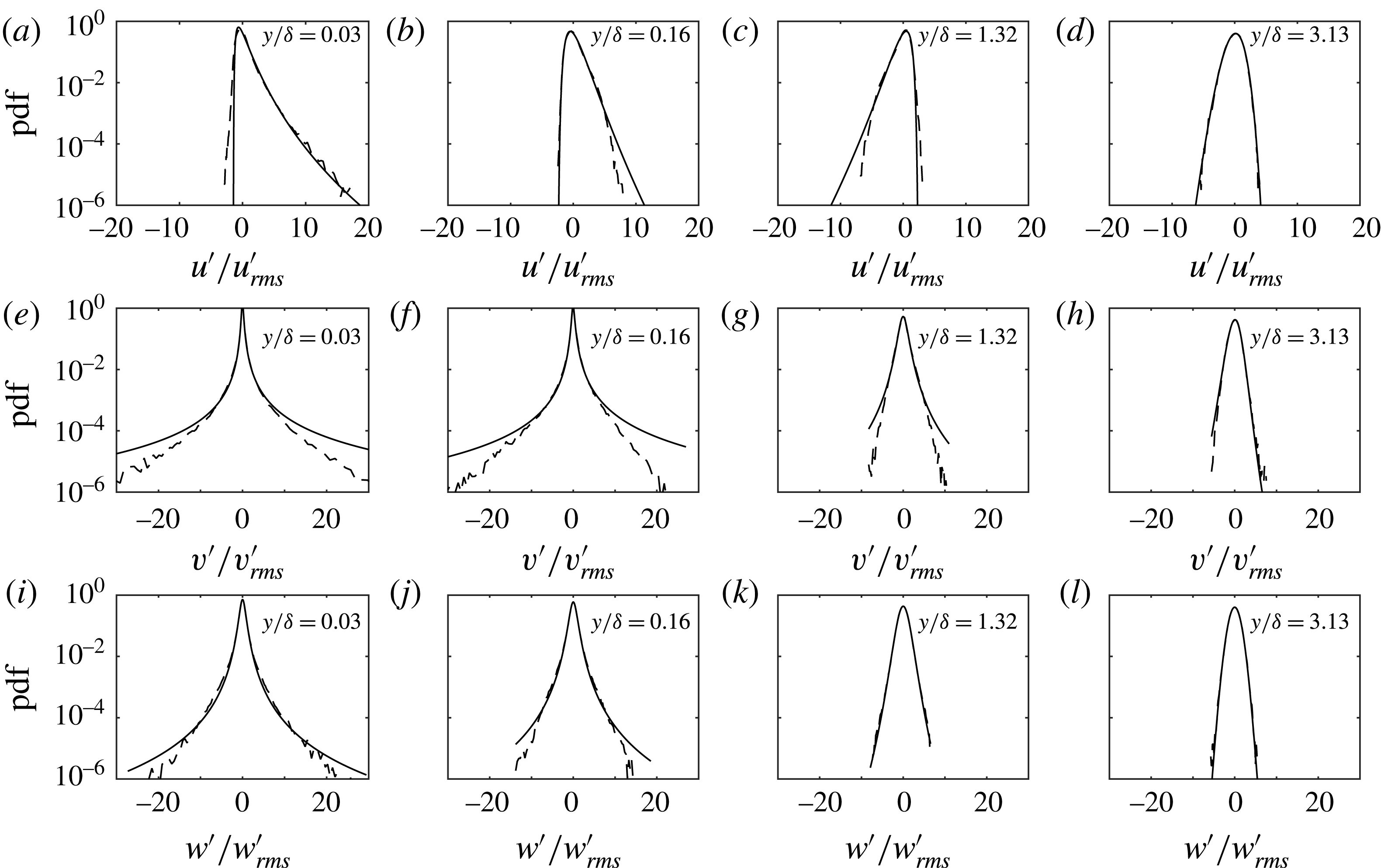
Figure 22 shows the time variation of the parameters of the distribution throughout the flow cycle for the three velocity components at the elevation closest to the wall (
 $y/\unicode[STIX]{x1D6FF}=0.03$
) and at an elevation further away (
 $y/\unicode[STIX]{x1D6FF}=1.32$
); both correspond to those shown before in figure 21. The equations and corresponding parameters for the log-normal and the Pearson type VII distributions can be found in Scandura et al. (Reference Scandura, Faraci and Foti2016) and are not be repeated here. Closest to the wall the parameters are relatively constant throughout the flow cycle, with exceptions at phases when the transition to turbulent flow occurs and around flow reversal. At
 $y/\unicode[STIX]{x1D6FF}=1.32$
the parameters generally show more time variation but also have larger values, while for the phases not shown at
 $y/\unicode[STIX]{x1D6FF}=1.32$
the normal distribution provided a better fit to the data. This information could be of practical use in the stochastic turbulence models outlined in the introduction to this paper. Current models assume a normal distribution of turbulence, but based on these results, the log-normal, Pearson type IV and Pearson type VII distributions provide better descriptions, particularly close to the wall. As a first approximation, close to the wall, the parameters of the distributions can be assumed constant throughout the flow cycle, and therefore will only be a function of elevation above the wall.
Time variation of the parameters of the log-normal (a,b), Pearson type IV (c,d), Pearson type VII distributions (e,f) to describe the pdf of the
 $u^{\prime }$
,
 $v^{\prime }$
and
 $w^{\prime }$
fluctuations, respectively; (a,c,e)
 $y/\unicode[STIX]{x1D6FF}=0.03$
, (b,d,f)
 $y/\unicode[STIX]{x1D6FF}=1.32$
. For phases not shown in (b) and (f) the normal distribution provided the best fit.
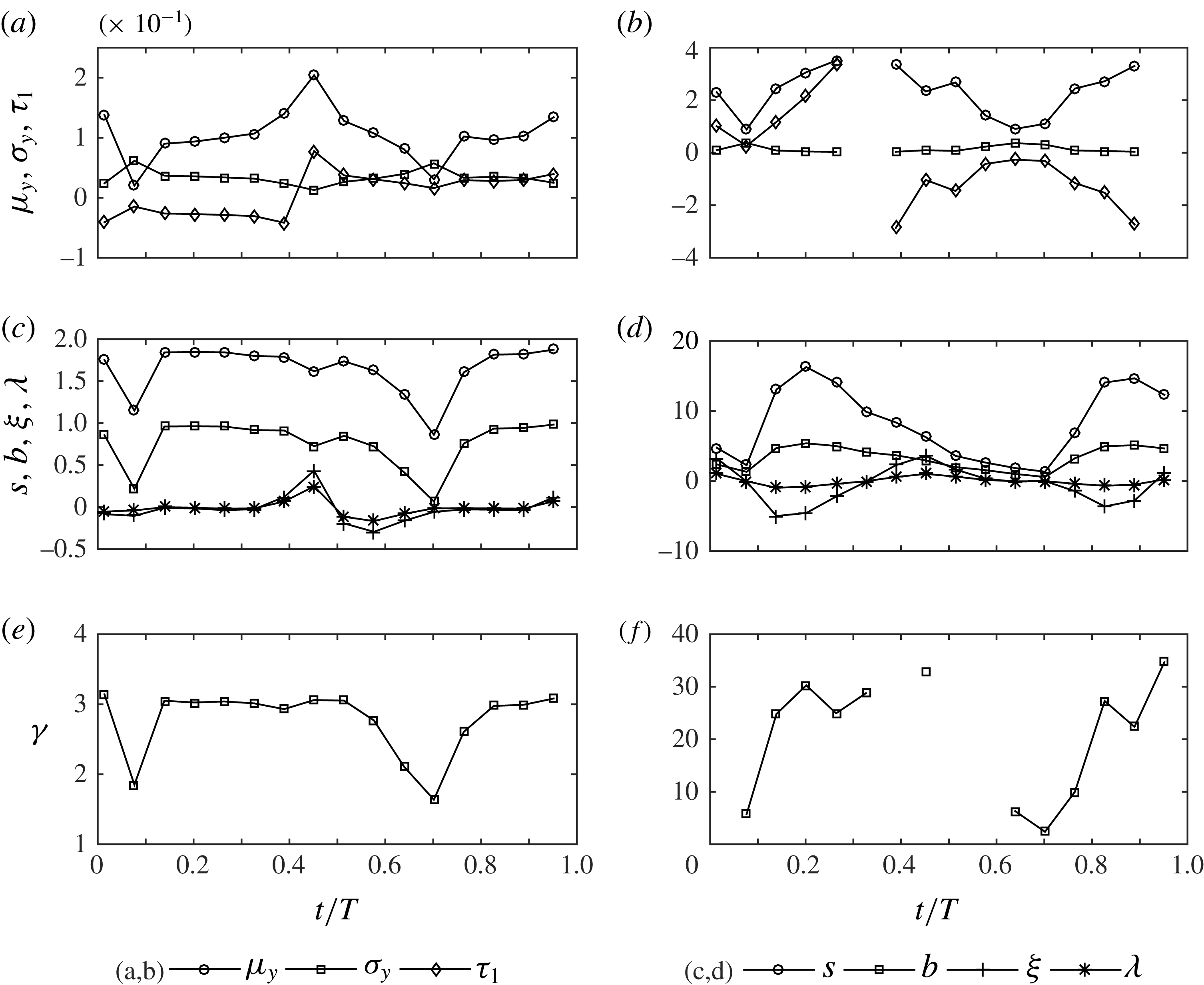
The correlations between streamwise and wall-normal velocity fluctuations can be analysed through the joint probability density functions (jpdf) of
 $u^{\prime }/u_{rms}^{\prime }$
and
 $v^{\prime }/v_{rms}^{\prime }$
shown in figures 23 and 24. The jpdf of
 $(u^{\prime },v^{\prime })$
is defined as
 $jpdf=m/(M\unicode[STIX]{x0394}u^{\prime }\unicode[STIX]{x0394}v^{\prime })$
, with
 $m$
the number of
 $(u^{\prime },v^{\prime })$
pairs falling within the interval
 $\unicode[STIX]{x0394}u^{\prime }\unicode[STIX]{x0394}v^{\prime }$
and
 $M=180$
. In these figures the values of the contour lines have been fixed according to the formula
 $10^{-0.6(l+n-2)}$
, where
 $n=1,2,\ldots$
are integer numbers denoting the contour lines and
 $l$
depends on
 $t/T$
and
 $y/\unicode[STIX]{x1D6FF}$
and is reported in the figure caption. Figure 23 shows the jpdf at phase
 $t/T=0.08$
for the same elevations considered in figures 19 and 20. It can be observed that very close to the wall (figure 23
a) large streamwise velocity fluctuations are correlated with large negative wall-normal velocity fluctuations. This is consistent with the existence of high-speed streaks generated by downward motions of fast fluid. The largest negative streamwise velocity fluctuations occur for small values of
 $v^{\prime }/v_{rms}^{\prime }$
, highlighting the fact that the largest positive values of
 $v^{\prime }/v_{rms}^{\prime }$
do not occur in the low-speed streaks but, as shown in figure 23(a), at locations between the low- and high-speed streaks.
The correlation between high positive values of
 $u^{\prime }/u_{rms}^{\prime }$
and high negative values of
 $v^{\prime }/v_{rms}^{\prime }$
seen for
 $y/\unicode[STIX]{x1D6FF}=0.033$
become weaker at
 $y/\unicode[STIX]{x1D6FF}=0.16$
(figure 23
b). Here both positive and negative peaks in
 $v^{\prime }/v_{rms}^{\prime }$
correlate with lower values of
 $u^{\prime }/u_{rms}^{\prime }$
, compared with
 $y/\unicode[STIX]{x1D6FF}=0.03$
. The largest positive values of
 $v^{\prime }/v_{rms}^{\prime }$
are now well correlated with vanishing fluctuations of the streamwise velocity. This result agrees with figure 11 of Scandura et al. (Reference Scandura, Faraci and Foti2016), which showed the existence of several positive peaks in
 $v^{\prime }$
occurring when
 $u^{\prime }$
is small. At larger
 $y/\unicode[STIX]{x1D6FF}$
, large positive
 $v^{\prime }/v_{rms}^{\prime }$
becomes correlated with negative
 $u^{\prime }/u_{rms}^{\prime }$
.
Joint probability density of streamwise and wall-normal velocity fluctuations at
 $t/T=0.08$
. At this phase the flow is dominated by elongated low-speed streaks. The contour lines are given by
 $10^{-0.6(l+n-2)}$
; (a)
 $y/\unicode[STIX]{x1D6FF}=0.033$
,
 $l=2$
, (b)
 $y/\unicode[STIX]{x1D6FF}=0.16$
,
 $l=2$
, (c)
 $y/\unicode[STIX]{x1D6FF}=1.32$
,
 $l=2$
, (d)
 $y/\unicode[STIX]{x1D6FF}=3.13$
,
 $l=3$
;
 $R_{\unicode[STIX]{x1D6FF}}=1155$
.
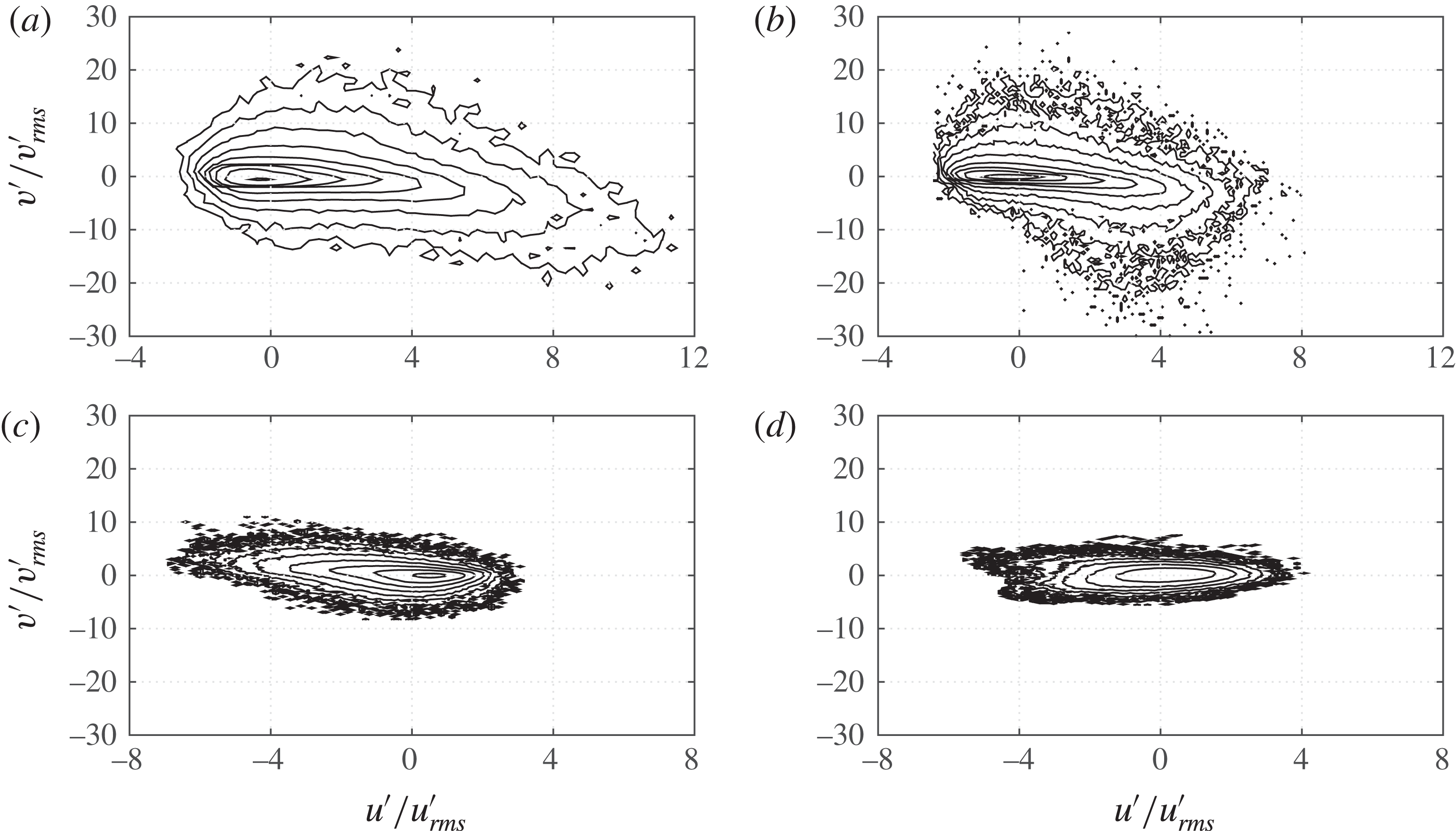
Joint probability density of streamwise and wall-normal velocity fluctuations at
 $t/T=0.14$
. At this phase breaking of the low-speed streaks has already occurred. The contour lines are given by
 $10^{-0.6(l+n-2)}$
; (a)
 $y/\unicode[STIX]{x1D6FF}=0.033$
,
 $l=2$
, (b)
 $y/\unicode[STIX]{x1D6FF}=0.16$
,
 $l=3$
, (c)
 $y/\unicode[STIX]{x1D6FF}=1.32$
,
 $l=3$
, (d)
 $y/\unicode[STIX]{x1D6FF}=3.13$
,
 $l=3$
;
 $R_{\unicode[STIX]{x1D6FF}}=1155$
.
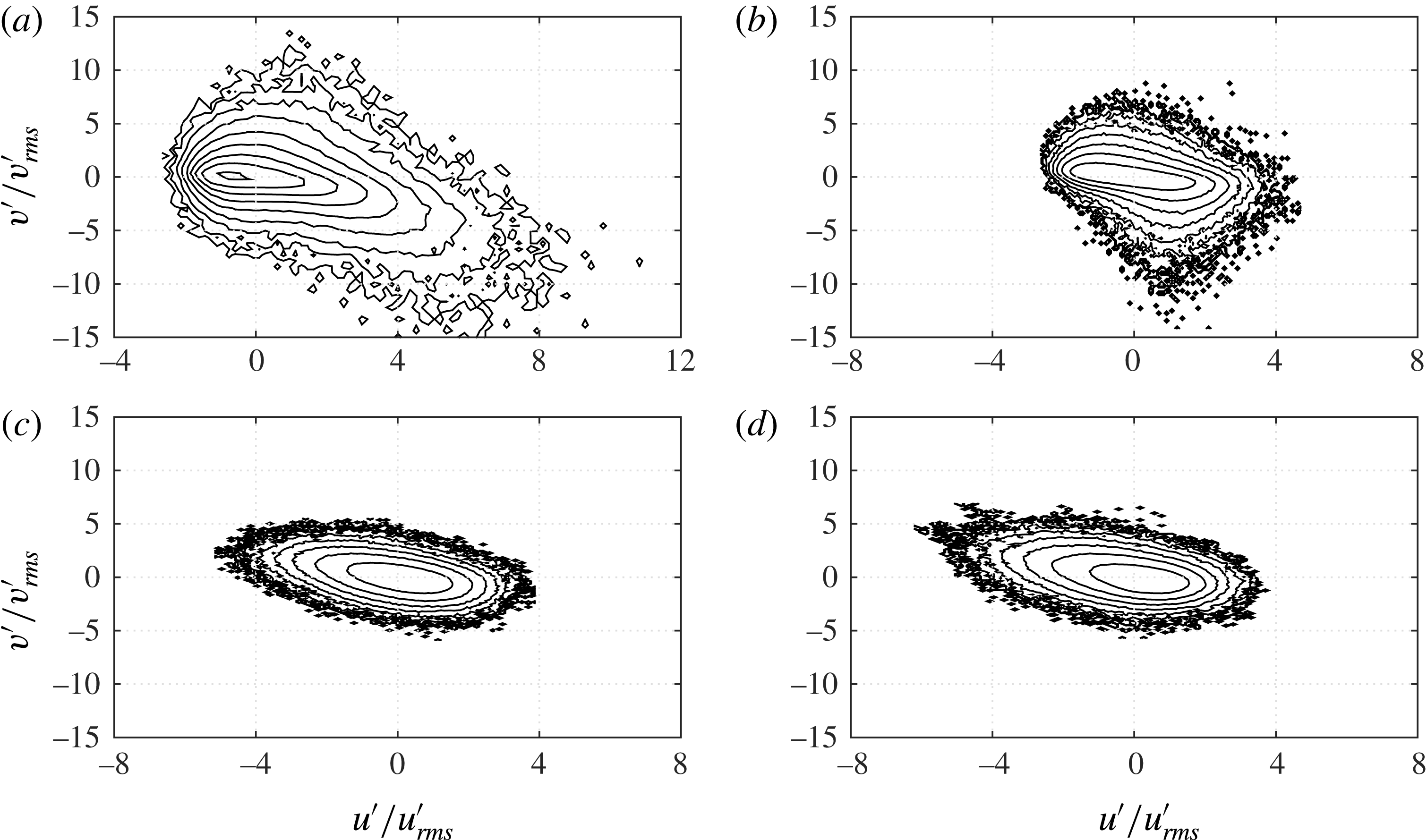
In figure 24 the jpdfs are shown for
 $t/T=0.14$
, i.e. following low-speed streak breaking. The results show a significant decrease in the dimensionless velocity fluctuations compared to the corresponding results for
 $t/T=0.08$
(figure 23). Both positive and negative peaks in
 $v^{\prime }/v_{rms}^{\prime }$
correlate with lower values of
 $u^{\prime }/u_{rms}^{\prime }$
compared with
 $t/T=0.08$
. In particular at
 $y/\unicode[STIX]{x1D6FF}=0.16$
the positive peak of
 $v^{\prime }/v_{rms}^{\prime }$
now occurs for negative values of
 $u^{\prime }/u_{rms}^{\prime }$
. In summary, with increasing distances from the wall the positive peak in
 $v^{\prime }/v_{rms}^{\prime }$
shifts from medium positive values of
 $u^{\prime }/u_{rms}^{\prime }$
towards negative values. At the same time the extreme negative fluctuations of
 $v^{\prime }/v_{rms}^{\prime }$
also shift towards low values of
 $u^{\prime }/u_{rms}^{\prime }$
.
Comparison between experimental and DNS results for Reynolds stress. (a)
 $R_{\unicode[STIX]{x1D6FF}}=1155$
, (b)
 $R_{\unicode[STIX]{x1D6FF}}=1475$
.
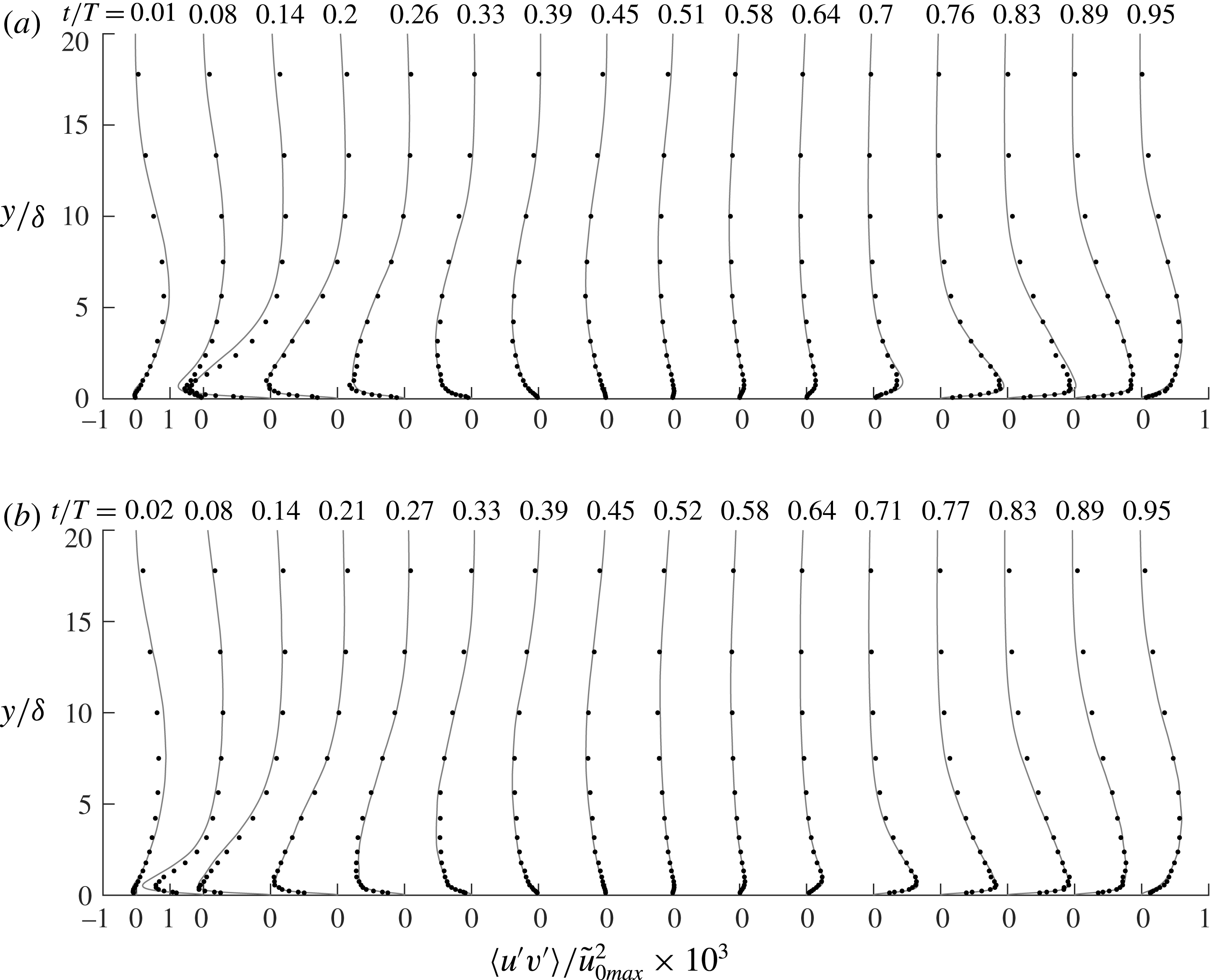
4.6 Reynolds stresses
The Reynolds stress
 $\langle u^{\prime }v^{\prime }\rangle$
can be computed as follows:
 $$\begin{eqnarray}\displaystyle \langle u^{\prime }v^{\prime }\rangle =\int _{-\infty }^{\infty }\int _{-\infty }^{\infty }\text{jpdf}~u^{\prime }v^{\prime }\,\text{d}u^{\prime }\,\text{d}v^{\prime }. & & \displaystyle\end{eqnarray}$$
In figure 25 the experimental and numerical Reynolds stresses are compared for
 $R_{\unicode[STIX]{x1D6FF}}=1155$
and
 $R_{\unicode[STIX]{x1D6FF}}=1475$
. The agreement between the experimental and numerical results is in general very good, with the exception of the near-wall measurements at phases
 $t/T=0.08$
, where the discrepancy may be due to the displacement of the glass side walls under high pressure, as explained previously. Additionally, as discussed in § 4.4, at these phases the turbulence is highly intermittent, therefore the discrepancy may be due to the limited sample size, even when measuring for 200 flow cycles. It can be seen that at the beginning of the flow cycle the Reynolds stress is positive and reaches a maximum at approximately
 $y/\unicode[STIX]{x1D6FF}=5$
. At this phase the Reynolds stress close to the wall (
 $y/\unicode[STIX]{x1D6FF}<2$
) is very small, but it quickly becomes negative and by
 $t/T=0.14$
it reaches a maximum at about
 $y/\unicode[STIX]{x1D6FF}=0.5$
. For the remaining phases the peak Reynolds stress decreases near the wall and moves upwards. During the negative half-cycle a similar process occurs, but because of the flow asymmetry the maximum stress occurs later in the half-cycle, and with lower magnitude compared to the positive half-cycle. However, because the maximum stress occurs later in the cycle the positive Reynolds stress that carries over in the subsequent half-cycle is much larger compared to the negative Reynolds stress that gets carried over into the negative half-cycle; compare for example the profiles at
 $t/T=0.08$
and
 $t/T=0.51$
in figure 25(a).
If the integration in (4.4) is carried out separately in each of the four quadrants (
 $Q_{1},Q_{2},Q_{3},Q_{4}$
) of the reference system, the contributions to the Reynolds stress from each quadrant are obtained. Quadrants can be distinguished as gradient type or counter-gradient type (Wallace Reference Wallace2016). Gradient type means that the vertical momentum flux
 $\unicode[STIX]{x1D70C}\langle u^{\prime }v^{\prime }\rangle$
is generated by particles that fluctuate in the
 $y$
direction and carry a streamwise momentum larger or smaller than the local mean momentum, depending on the local mean velocity gradient. Following this definition, when the mean velocity gradient is positive, the fluctuation products
 $u^{\prime }v^{\prime }$
in gradient type quadrants are negative; hence gradient type quadrants are
 $Q_{2}$
and
 $Q_{4}$
and counter-gradient type quadrants are
 $Q_{1}$
and
 $Q_{3}$
. The opposite occurs if the mean velocity gradient is negative. Note that in unsteady flows the sign of the mean velocity gradient is not constant in the
 $y$
direction, hence the type of gradient quadrant may change in the vertical direction.
How much each quadrant contributes to the Reynolds stress is shown in figure 26 for
 $R_{\unicode[STIX]{x1D6FF}}=1155$
. The rectangle on the left side of each panel shows the locations above the wall where the gradient of the ensemble-averaged velocity is positive. It can be observed that in the positive half-cycle, close to the wall, gradient type quadrants are
 $Q_{2}$
and
 $Q_{4}$
while far from the wall gradient type quadrants are
 $Q_{1}$
and
 $Q_{3}$
. Generally, the contributions of the gradient type quadrants dominate and the Reynolds stress is negative if gradient type quadrants are
 $Q_{2}$
and
 $Q_{4}$
, while it is positive if gradient type quadrants are
 $Q_{1}$
and
 $Q_{3}$
.
It can also be observed that close to the wall
 $Q_{4}$
provides the largest contribution to the Reynolds stress, but at higher elevations
 $Q_{2}$
becomes more important.
When the flow moves towards flow reversal and the turbulence decays,
 $\langle u^{\prime }v^{\prime }\rangle _{Q_{2}}$
and
 $\langle u^{\prime }v^{\prime }\rangle _{Q_{4}}$
become very close to each other. In the negative half-cycle
 $Q_{1}$
and
 $Q_{3}$
are gradient type close to the wall while far from the wall
 $Q_{2}$
and
 $Q_{4}$
are gradient type. The
 $Q_{3}$
contribution is largest very close to the wall and the
 $Q_{1}$
contribution is the largest far from the wall. Again, the two contributions become similar as flow reversal is approached.
Reynolds stress and quadrant contributions to the Reynolds stress for
 $R_{\unicode[STIX]{x1D6FF}}=1155$
. The rectangle on the left side of each panel denotes the locations where the gradient of the mean velocity is positive.
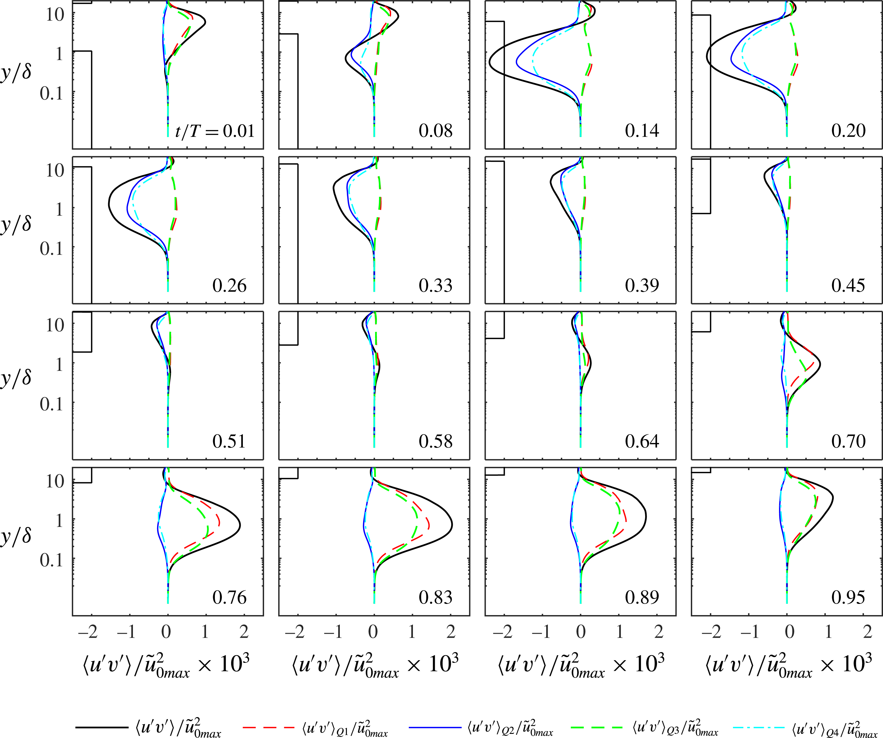
A budget analysis provides insights into the generation and transport mechanisms of the Reynolds stress. For the flow under consideration the Reynolds stress budget can be written as follows (see Pope Reference Pope2000):
 $$\begin{eqnarray}\displaystyle \frac{\unicode[STIX]{x2202}\langle u^{\prime }v^{\prime }\rangle }{\unicode[STIX]{x2202}t} & = & \displaystyle -\langle v^{\prime 2}\rangle \frac{\unicode[STIX]{x2202}\langle u\rangle }{\unicode[STIX]{x2202}y}-\frac{\unicode[STIX]{x2202}\langle u^{\prime }v^{\prime 2}\rangle }{\unicode[STIX]{x2202}y}-\frac{1}{\unicode[STIX]{x1D70C}}\left\langle v^{\prime }\frac{\unicode[STIX]{x2202}p^{\prime }}{\unicode[STIX]{x2202}x}+u^{\prime }\frac{\unicode[STIX]{x2202}p^{\prime }}{\unicode[STIX]{x2202}y}\right\rangle +\unicode[STIX]{x1D708}\frac{\unicode[STIX]{x2202}\langle u^{\prime }v^{\prime }\rangle }{\unicode[STIX]{x2202}y^{2}}\nonumber\\ \displaystyle & & \displaystyle -\,2\unicode[STIX]{x1D708}\left\langle \frac{\unicode[STIX]{x2202}u^{\prime }}{\unicode[STIX]{x2202}x}\frac{\unicode[STIX]{x2202}v^{\prime }}{\unicode[STIX]{x2202}x}+\frac{\unicode[STIX]{x2202}u^{\prime }}{\unicode[STIX]{x2202}y}\frac{\unicode[STIX]{x2202}v^{\prime }}{\unicode[STIX]{x2202}y}+\frac{\unicode[STIX]{x2202}u^{\prime }}{\unicode[STIX]{x2202}z}\frac{\unicode[STIX]{x2202}v^{\prime }}{\unicode[STIX]{x2202}z}\right\rangle .\end{eqnarray}$$
The terms on the right-hand side of (4.5) correspond to production, turbulent diffusion, velocity pressure gradient, viscous diffusion and dissipation.
Figure 27 shows the budget terms through the flow cycle for
 $R_{\unicode[STIX]{x1D6FF}}=1155$
. At the beginning of the flow cycle (
 $t/T=0.01$
) all terms of (4.5) are very small. As the flow accelerates (
 $t/T=0.08$
) production emerges as the largest term far from the wall. The sign of production is opposite to that of the mean velocity gradient, therefore in the first half-cycle it is mostly negative close to the wall and slightly positive at large
 $y/\unicode[STIX]{x1D6FF}$
. Far from the wall the second most important term is the velocity pressure-gradient term which is of opposite sign to production at all elevations and phases. Very close to the wall (
 $0<y/\unicode[STIX]{x1D6FF}<0.1$
), the transport of the Reynolds stress is mainly due to viscous diffusion. In the same range of
 $y/\unicode[STIX]{x1D6FF}$
turbulent diffusion is small and approximately follows production. The similarity between production and turbulent diffusion can be justified by realising that both terms vary as
 $y^{4}$
as
 $y$
tends to zero, which results from expanding the velocity components in a Taylor series. For
 $R_{\unicode[STIX]{x1D6FF}}=1475$
, the budget of the Reynolds stress (not shown) exhibits most of the features described above, but the phases at which the budget terms become large occur earlier in the flow half-cycles compared to the phases for
 $R_{\unicode[STIX]{x1D6FF}}=1155$
. For example, at
 $t/T=0.08$
the magnitude of the budget terms for
 $R_{\unicode[STIX]{x1D6FF}}=1475$
are similar to those shown in figure 27 for
 $t/T=0.14$
.
The flow asymmetry has clear effects on the Reynolds stress budget. In the negative half-cycle the phase at which the budget terms obtain significant values occurs later compared to the first half-cycle. On the other hand, in the negative half-cycle the budget terms remain significant until near flow reversal (
 $t/T=0.95$
), while at the end of the positive half-cycle they are very small.
Terms of the Reynolds stress budget made dimensionless by
 $\tilde{u} _{0max}^{2}\unicode[STIX]{x1D70E}$
for
 $R_{\unicode[STIX]{x1D6FF}}=1155$
(see (4.5)). DNS data.
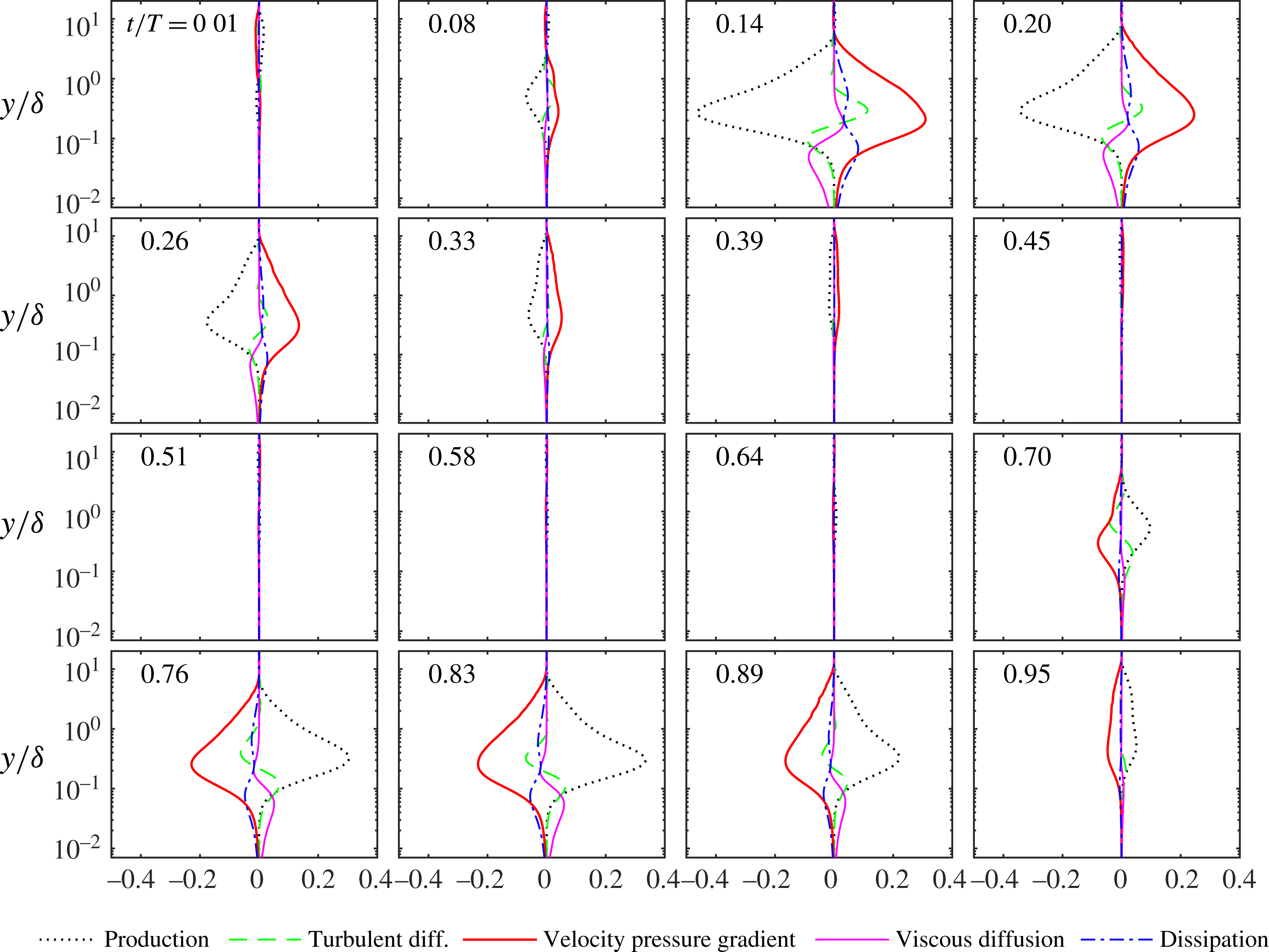
5 Conclusions
The velocity statistics of an asymmetric oscillatory flow over a smooth wall have been analysed by means of experiments in a large oscillating flow tunnel and direct numerical simulations. The experiments were performed for five Reynolds numbers (
 $R_{\unicode[STIX]{x1D6FF}}$
) ranging from 846 to 2057, while the numerical simulations were performed for
 $R_{\unicode[STIX]{x1D6FF}}$
equal to 846, 1155 and 1475. The main results of the study are summarised in the following.
Since the experimental facility is a closed system, and the numerical simulations were carried out for an infinitely long periodic domain, the two flows differ in terms of the period-averaged quantities. In the numerical simulations the period-averaged streamwise velocity (boundary layer streaming), is opposite to the streamwise direction, tends to a constant for
 $y/\unicode[STIX]{x1D6FF}$
far from the wall and its gradient vanishes at
 $y/\unicode[STIX]{x1D6FF}=0$
. The boundary layer streaming results from the asymmetry in the oscillatory flow, which produces a non-zero mean Reynolds stress. This negative streaming also exists in the oscillating flow tunnel, but in this case it is balanced by a positive current driven by a negative pressure gradient. Thus a positive mean shear stress is applied to the wall of the oscillating flow tunnel. The experimental verification of this finding is here provided for the first time.
The agreement between experimental and numerical vertical profiles of velocity is good, once the time-averaged velocity is subtracted. This shows that the magnitude of the streaming is not strong enough to significantly affect the oscillatory component of the phase-averaged velocity. This is also confirmed by the good agreement between experiments and numerical simulations in terms of the periodic component of the Reynolds stress.
Because of the asymmetry in the free-stream velocity, the magnitude of the positive half-cycle peak wall shear stress exceeds that of the negative half-cycle. The experimental and DNS results for wall shear stress are in good agreement and show that the asymmetry coefficient for the wall shear stress, defined as
 $(\unicode[STIX]{x1D70F}_{max}+\unicode[STIX]{x1D70F}_{min})/\unicode[STIX]{x1D70F}_{max}$
, increases with Reynolds number.
Good agreement between experiments and numerical simulations has been observed in terms of the lower- and higher-order statistics of the velocity fluctuations, especially for the higher Reynolds number flow. Close to the wall the relative intensity of
 $u^{\prime }~(\langle u^{\prime 2}\rangle /|\tilde{u} |)$
increases during the accelerating phase, attains a maximum value of about 0.48, and subsequently decreases to a value of about 0.4, which is maintained for much of the remainder of the half-cycle. The skewness and the flatness of
 $u^{\prime }$
increase during the accelerating phase and reach maximum values at the onset of breaking of low-speed streaks in the fluid domain. In both half-cycles there is excellent agreement between experiments and numerical simulations concerning the phase at which both skewness and flatness attain their peak values. Once maximum values have been reached, the higher-order statistics rapidly decrease until the phase at which the flow domain is filled with breaking low-speed streaks. The phase of inception of the low-speed streaks breaking,
 $\unicode[STIX]{x1D719}_{1}$
, and the phase at which the breaking is complete,
 $\unicode[STIX]{x1D719}_{2}$
, are shown to depend on the Reynolds number. As Reynolds number increases,
 $\unicode[STIX]{x1D719}_{1}$
and
 $\unicode[STIX]{x1D719}_{2}$
shift to earlier in each half-cycle and the time between the onset and completion of breaking (
 $\unicode[STIX]{x1D719}_{2}-\unicode[STIX]{x1D719}_{1}$
) decreases.
The skewness of the streamwise velocity fluctuations is small at elevations above the wall where
 $\unicode[STIX]{x2202}\langle u\rangle /\unicode[STIX]{x2202}y=0$
. At the same elevations the flatness takes a value of approximately 3. Generally, the flatness remains close to 3 and the skewness close to zero for elevations above
 $y/\unicode[STIX]{x1D6FF}$
corresponding to
 $\unicode[STIX]{x2202}\langle u\rangle /\unicode[STIX]{x2202}y=0$
. Therefore, within this range the streamwise velocity fluctuations are close to being normally distributed. Close to the wall, both the skewness and the flatness are high, as well as their wall-normal gradient; in particular, during transition to turbulence the flatness of the wall-normal velocity fluctuation is of order
 $10^{2}$
. The reason for this is the spatial intermittency of the wall-normal fluctuations, i.e. localised large velocity fluctuations are separated by large areas where the velocity fluctuations are small. This phenomenon results in long tails in the probability density functions, generated by extremely large values with low probability. In the pdf of the streamwise velocity fluctuations the positive tail is much larger than the negative tail. The positive tail reduces rapidly with
 $y/\unicode[STIX]{x1D6FF}$
, resulting in a large wall-normal gradient in the statistics. In contrast, the negative tails remain rather constant with increasing
 $y/\unicode[STIX]{x1D6FF}$
.
Comparing the probability distributions of the fluctuating velocities from DNS with theoretical probability density functions has shown that the streamwise velocity fluctuations are well described by a log-normal distribution, the wall-normal velocity fluctuations are well described by the Pearson type IV distribution and the spanwise velocity fluctuations are well described by the Pearson type VII distribution.
The joint probability density of
 $u^{\prime }$
and
 $v^{\prime }$
shows that, close to the wall, large negative
 $v^{\prime }$
correlate with large positive
 $u^{\prime }$
while large positive
 $v^{\prime }$
correlate with medium values of
 $u^{\prime }$
. Moving away from the wall, these correlations shift to lower values of
 $u^{\prime }$
. Negative
 $v^{\prime }$
occurring with positive
 $u^{\prime }$
and positive
 $v^{\prime }$
occurring with low or negative
 $u^{\prime }$
is consistent with the presence of streamwise vortices ejecting low-speed fluid away from the wall and high-speed fluid towards the wall (Scandura et al.
Reference Scandura, Faraci and Foti2016).
Experimental and numerical vertical profiles of Reynolds stress show good agreement, except at phases corresponding to high pressure in the tunnel, which causes deformation of the glass side walls and affects the accuracy of the near-bed measurements where the gradient is large.
The largest contribution to the Reynolds stress arises from the gradient type quadrants at all phases.
 $Q_{2}$
and
 $Q_{4}$
provide the largest contribution in the positive half-cycle, while
 $Q_{1}$
and
 $Q_{3}$
do so in the negative half-cycle. The contribution of
 $Q_{4}$
(
 $Q_{3}$
) is largest close to the wall and that of
 $Q_{2}$
(
 $Q_{1}$
) is largest far from the wall. During flow deceleration, the contributions of these two quadrants tend to become equal. The counter-gradient quadrants provide approximately equal contributions at all phases. The Reynolds stress budget shows that production and velocity pressure-gradient terms are the largest for
 $y/\unicode[STIX]{x1D6FF}>0.1$
and generally are of opposite sign throughout the boundary layer and at all phases. For
 $y/\unicode[STIX]{x1D6FF}<0.1$
viscous diffusion is positive and larger than the other terms, hence it represents the main mechanisms by which large Reynolds stress occurs close to the wall. In the same range of
 $y/\unicode[STIX]{x1D6FF}$
, turbulent diffusion is positive and closely follows production, because these terms have similar asymptotic behaviour for
 $y/\unicode[STIX]{x1D6FF}$
tending to zero.
Acknowledgements
This work has been carried out within the SINBAD project, funded through the UK Engineering and Physical Sciences Research Council (EPSRC grant EP/J00507X/1). P.S. acknowledges the funding from the University of Aberdeen to support his Honorary Research Fellowship and funding from the Ministero dell’Istruzione dell’Università e della Ricerca through PRIN 2012 ‘Hydromorphodynamic and modeling of coastal processes for engineering purposes’. The authors acknowledge the support of the technical staff at the University of Aberdeen, especially Fluids Laboratory Technician Roy Gillanders. The experimental and numerical datasets presented in this paper are available on https://dx.doi.org/10.5281/zenodo.1095116.



