



Nomenclature
- AMOT
-
allowable material operating temperature
- APPU
-
auxiliary propulsion and power unit
- APU
-
auxiliary power unit
- HE
-
heat exchanger
- LHV
-
lower heating value
- LTO
-
landing and take-off
- RQL
-
rich-burn quick-quench lean-burn
- SFC
-
specific fuel consumption
- SFC
 $_{corr}$
-
SFC, corrected for fuel temperature
- SIR
-
steam injection and recovery
- SP
-
specific power
- SR
-
splitting ratio
- TET
-
turbine entry temperature
- WAR
-
water-to-air ratio
-
$A$
-
area
-
${C_P}$
-
specific heat capacity
-
$E$
-
heat exchanger effectiveness
-
$h$
-
enthalpy
-
$P$
-
power
-
$p$
-
pressure
-
$Q$
-
heat transfer rate
-
$V$
-
water flow rate
-
$W$
-
mass flow rate
-
$\eta $
-
efficiency


1.0 Introduction
The growing demand for aviation makes it challenging to reduce its emissions. The aviation sector currently contributes about 4% to anthropogenic global warming [Reference Klöwer, Allen, Lee, Proud, Gallagher and Skowron1]. The number of passenger kilometers increases by approximately 4.8% per year. However, aircraft are also becoming more fuel-efficient. Fuel consumption per passenger kilometre has decreased by 75% since the 1960s, and about half of this reduction is the result of improved gas turbine efficiency [Reference Yin and Rao2]. The fuel burn per passenger kilometre is expected to reduce further by approximately 1.3% each year [Reference Yin and Rao3]. However, despite efficiency improvements, the result is that the climate impact of aviation will continue to grow, putting stress on parties involved in aircraft design and operations, as they will have to meet the emissions reduction targets set by the Advisory Council for Aeronautics Research and Innovation in Europe (ACARE) [4]. Part of this will come from the use of renewable fuels, such as sustainable aviation fuel and hydrogen, and part will come from improved aircraft technology and operational efficiency [Reference Klöwer, Allen, Lee, Proud, Gallagher and Skowron1, Reference Wells, Williams, Nichols, Kalise and Poll5–Reference Khandelwal, Karakurt, Sekaran, Sethi and Singh8].
To meet these objectives, radically different aircraft designs are proposed, such as blended-wing-body aircraft [Reference Brown and Vos9] and fully hydrogen-powered aircraft [Reference Kramer10]. The drawback of these concepts is that their entry into service (EIS) is expected to be around 2040–2050 [Reference Bravo-Mosquera, Catalano and Zingg11, 12]; an intermediate solution is required. The A321APPU is such a semi-radical intermediate solution, with an intended EIS in the next decade.
The A321 APPU project aims to reduce CO
 $_2$
and other harmful emissions by replacing the auxiliary power unit (APU) of an Airbus A321 with a hydrogen-powered auxiliary power and propulsion unit (APPU) [Reference Heidebrecht, Burger, Hoogreef, Vos, Isikveren and Rao13, Reference Heidebrecht, Hoogreef, Isikveren and Rao14]. The aim of the project is to reduce CO
 $_2$
emissions by 20% % while keeping the changes minimal [15]. As the APPU is an addition to the sufficiently powerful main engines, risks and requirements with respect to reliability and certification are reduced [Reference Heidebrecht, Burger, Hoogreef, Vos, Isikveren and Rao13, Reference Acevedo, van Cranenburgh, Exalto, Halsema, van der Heijden, Hoogterp, Jahilo, Jorge, Naäman, van Schie and van der Zwan16]. In addition to reducing cruise CO
 $_2$
emission, the emissions of the landing and take-off cycle (LTO) should be reduced by 50% [15]. The engine is located in the tail with an aft propeller. Unfortunately, the placement of the engine and the inlet results in a large pressure loss due to the boundary layer [Reference Heidebrecht, Burger, Hoogreef, Vos, Isikveren and Rao13, Reference Bariş17]. The intended architecture of the APPU engine is a three-spool turboshaft with a free turbine and mixed compressor (axial and radial) architecture. Figure 1 shows a rendering of the A320 APPU with an overview of the main characteristics of the aircraft [Reference Acevedo, van Cranenburgh, Exalto, Halsema, van der Heijden, Hoogterp, Jahilo, Jorge, Naäman, van Schie and van der Zwan16].
Rendering of the A320 APPU with key characteristics [Reference Acevedo, van Cranenburgh, Exalto, Halsema, van der Heijden, Hoogterp, Jahilo, Jorge, Naäman, van Schie and van der Zwan16].

In order to achieve and exceed these targets, the steam injection and recovery (SIR) cycle is applied. In this cycle, pressurised steam is injected into the combustor, and heat exchangers (HE) and a water collector are placed after the turbines, making it a semi-closed cycle. The liquid water collected is pressurised and subsequently heated and evaporated in the heat recovery steam generator (HRSG). The steam is then injected into the combustion chamber, starting the cycle over again. The application of this cycle in a turbofan engine has been analysed by Schmitz [Reference Schmitz, Klingels and Kufner18] and Kaiser [Reference Kaiser, Schmitz, Ziegler and Klingels19]. The SIR cycle offers improvements in specific fuel consumption (SFC) by utilising the incompressibility of liquid water for efficient compression and by recovering the heat from the exhaust [Reference Schmitz, Klingels and Kufner18]. These benefits are maximised by minimising the heat exchanger pressure losses. Another potential is the significant reduction of NO
 $_x$
emissions, which is a result of the lower peak combustion temperatures due to the injected steam [Reference Walsh and Fletcher20–Reference Chen, Maloney and Day22]. A drawback is the addition of weight and complexity by introducing these new components.
Whereas in the research by Schmitz [Reference Schmitz, Klingels and Kufner18] and Kaiser [Reference Kaiser, Schmitz, Ziegler and Klingels19], a cold bypass flow could be used to cool the core exhaust flow, but the SIR APPU needs a different heat sink. The only reasonable option is to use the liquid hydrogen fuel. However, this is not enough to sufficiently cool the entire exhaust flow; the flow can only be cooled by around 100 K [Reference van Schie23]. Therefore, the exhaust flow of the SIR APPU is divided into two paths – one going into the main gas path and the other to a path with the heat exchangers. The flow fraction in each is governed by the split ratio (SR) and Equation (1):
 \begin{align} SR = \frac{{{W_{HE}}}}{{{W_{main}}}} \end{align}
where
 $W$
is the mass flow rate in the respective ducts. The HE path contains the HRSG, the condenser and the collector. The HRSG is as described above. The condenser uses LH
 $_2$
to cool the flow and condense the water vapour so that it can be collected in the collector. The remainder of the water cycle is as described above. The remaining flow is mixed with the main gas path before exiting through the nozzle. A schematic of the SIR APPU architecture is shown in Fig. 2.
Schematic representation of the SIR APPU cycle.

This research aims to quantify the impact of the SIR cycle on the APPU performance. The scope is limited to the impact on SFC, NO
 $_x$
emissions and a rough estimation of the weight penalty. First, the methods used in the analysis are explained, after which the verification and validation practices are stated. The input and output of the analysis are then listed, followed by a discussion of the results. Lastly, the conclusions and recommendations are discussed.
2.0 Methodology
In order to quantify the impact of the SIR cycle, both the baseline and SIR APPU are analysed. Both engines are sized for the same power output in the design condition (meaning differently sized cores as the specific power (SP) varies). The two engines are compared for SFC, relative NO
 $_X$
emissions and mass. This section explains the methods used. First, the analysis tools used are mentioned, after which the required enhancement of the pyCycle tool is discussed.
2.1 Analysis tools
Gas turbines are complex machines with numerous dependencies between different components. Therefore, engine analysis tools are used. To limit the amount of input parameters needed, the engines are assessed by means of a parametric analysis. Various tools exist for this, and the following two are used: pyCycle and Gasturb.
pyCycle was created as an efficient engine analysis tool to be incorporated into multidisciplinary analysis and optimisation solutions and is based on NASA’s openMDAO framework [Reference Hendricks and Gray24–Reference Gray, Hwang, Martins, Moore and Naylor26]. The determination of the thermodynamic properties of the flow is done using an adaptation of NASA’s Chemical Equilibrium with Applications (CEA) method [Reference Gordon and McBride27–Reference Gray, Chin, Hearn, Hendricks, Lavelle and Martins29]. pyCycle is an open-source code and can thus easily be accessed and modified. The pyCycle models an engine by linking different components after each other and ensuring consistency between them in terms of mass and energy fluxes. This programme design allows the user to build their own architectures.
The other analysis tool used is Gasturb 12 [30], originally developed to automate parametric and performance cycle analyses and find optimal cycle parameters [Reference Kurzke31]. It can also assist in more detailed aspects of the engine, such as preliminary component sizing and mass estimation. The user can select from a number of predetermined engine cycles, which cannot be altered. This means that the SIR cycle cannot be modelled in Gasturb. However, the baseline APPU (a two-spool free power turbine turboshaft engine) is available and can be used to verify the pyCycle model.
Gasturb is also used for the (core) mass estimation. The total mass of the baseline APPU can be calculated by Gasturb. Equation (2) is used to estimate the mass of the SIR APPU. As the conventional parts of the SIR APPU are similar but slightly differently sized, the baseline mass is linearly scaled with the inlet mass flow rate to get the SIR APPU core mass. In order to do this, the mass of the new HEs is added. The determination of HE masses is explained in Subsection 3.3. The mass of the condenser and any additional ducting due to the two separate gas paths have not been included because an approximate method could not be found, and a detailed design is out of scope for this research.
 \begin{align} {m_{SIRAPPU}} = \frac{{{W_{SIR}}}}{{{W_{APPU}}}}{m_{APPU}} + {m_{HEs}}\end{align}
In their current state, both tools cannot yet model the SIR cycle. Because pyCycle can be enhanced with custom-built components, it is used for the main analyses. After adding the required components, both the baseline and SIR cycles are modelled and compared. Gasturb is used to verify the correct functioning of the baseline model in pyCycle. Additionally, Gasturb is used to estimate the motor mass.
2.2 Turbomachinery efficiencies
An important aspect of a gas turbine is the efficiency of the components of the turbomachinery. These have a significant impact on the performance of the engine. Therefore, it is important to establish and use the appropriate efficiency. These are influenced by the type of compressor or turbine, the size, the level of technology and the amount of turbine cooling air. To allow for later modifications and determinations of engine parameters, such as pressure ratios, turbine entry temperature (TET) and allowable material operating temperature (AMOT) of the turbines, a method was developed to determine the efficiency based on a few component parameters.
The efficiency of the baseline component was determined based on the corrected mass flow rate on the small side of the component (compressor exit and turbine inlet). For this, data from Snyder and Tong [Reference Snyder and Tong32] was used, which is shown in Fig. 3. This data includes the efficiency discrepancy between axial and centrifugal compressors and blends it into one continuous data set. The ‘Advanced’ technology level is used for the analyses, as the intended EIS is still some years away.
Component efficiency as a function of corrected mass flow for different technology levels with their respective fitted curves (data from Ref. [Reference Snyder and Tong32]).

This base efficiency is used for compressors, but turbines require the determination of the cooling air requirement and its impact. The required cooling air fraction is determined with a method from Jonssen et al. [Reference Jonsson, Bolland, Bücker and Rost33]. This method requires only the temperature of the coolant, the incoming flow and the AMOT. The latter is set at 1450 K [Reference Yin and Rao3, Reference Yin, Tiemstra and Rao34]. According to Yin and Gangoli Rao [Reference Yin and Rao3], every 1% cooling air fraction lowers the turbine efficiency by 0.6%. These aspects are factored in to obtain the final turbine efficiency. More detailed information on this method and its implementation can be found in Ref. [Reference van Schie23].
2.3 Modelling in pyCycle
In its current publicly available version, pyCycle is not able to model the SIR cycle because it lacks the capability to model liquid water and the phase change, there are no HE and water collection components available, and a modified combustor that is able to inject (partial) steam needs to be implemented. The HRSG, condenser and collector are entirely new components added to pyCycle, and the combustor is an altered version of the original. The nature of pyCycle allows these new components to be linked to an engine of conventional components. This subsection describes the workings inside the new components, as well as the determination of the main HE parameters.
The CEA implementation in pyCycle is able to model water vapour at various pressures and temperatures, but not liquid water and its phase change. The thermodynamic properties of the pure water flow in HRSG, such as enthalpy, latent heat and boiling temperature, are determined using the IAPWS-97IF method [Reference Cooper and Dooley35]. The condensation process in the condenser is governed by the relative humidity method described by Sonntag [Reference Sonntag36], and the latent heat released is determined using the IAPWS-97IF method.
Two key components of the SIR cycle are the heat exchangers: the HRSG and the condenser. Both are envisioned to be counterflow heat exchangers. This means that theoretically, the hot-side outflow can be as cold as the cold-side inflow, and vice versa. The heat transferred is governed by Equation (3):
 \begin{align} E = \frac{{{W_h}( {{h_{in,h}} - {h_{out,h}}} )}}{{{Q_{max}}}} = \frac{{{W_c}( {{h_{out,c}} - {h_{in,c}}} )}}{{{Q_{max}}}}\end{align}
where
 \begin{align*} \left. {\begin{array}{*{20}{l}}{{Q_h} = {W_h}( {{h_{in,h}} - {h_{h,{T_{in,c}}}}} )}\\{{Q_c} = {W_c}( {{h_{h,{T_{in,h}}}} - {h_{in,c}}} )}\end{array}} \right\}{Q_{max}} = MIN( {{Q_h},{Q_c}} )\end{align*}
Here,
 $E$
is the effectiveness of the heat exchanger, the fraction of the theoretical maximum heat transfer
 ${Q_{max}}$
that occurs.
 $W$
denotes the mass flow rate and
 $h$
is the specific enthalpy of the flow. The subscripts
 $h$
and
 $c$
indicate the hot and cold flow, respectively. The convenience of using the specific enthalpy over a specific heat and temperature is that any variation in specific heat is taken into account, as well as the latent heat of a phase change. The flow parameters on both sides are known, and
 $E$
is a design parameter set by the user, allowing quantification of the heat transfer rate and subsequently of the outflow parameters.
It is found that for the current HRSG application, there is not sufficient heat transfer to evaporate all the water, meaning that a mixture of water and steam is injected into the combustor, thereby creating the need to add a modified combustor.
The next heat exchanger in the SIR cycle is the condenser. This component further cools down the gas flow such that the water vapour condenses to liquid water, which subsequently can be collected. Liquid hydrogen (LH
 $_2$
) fuel is used as the heat sink for this process and is therefore the limiting factor in heat extraction. Hydrogen is assumed to enter the condenser in the liquid state, at 4.00 MPa and 20 K, above the critical pressure of hydrogen. The thermodynamic properties are taken from McCarty et al. [Reference McCarty, Hord and Order37]. The enthalpy difference between 20 K and 300 K is taken, and any variation from 300 K in temperature is approximated using a constant specific heat capacity of 14.50 kJ/kg K.
The final temperature of the exhaust gases is determined iteratively as a consequence of cooling. The amount of water condensed depends on the final temperature, but that temperature depends on the amount of water condensed. The iteration is complete when the following equation is true:
 \begin{align} {Q_{h2}} = {Q_{cooling}} + {Q_{condensation}}\end{align}
where
 ${Q_{h2}}$
is the achievable heat flow rate in hydrogen, and
 ${Q_{cooling}}$
and
 ${Q_{condensation}}$
are the heat flow rates attributed to the cooling of the flow and the extraction of latent heat, respectively.
The CEA model as implemented in pyCycle uses a lower temperature limit of 200 K, which is also enforced in the condenser to avoid numerical complications. This puts a limit on
 ${Q_{cooling}}$
and consequently on
 ${Q_{h2}}$
. The result is that the heat exchanger effectiveness of the condenser is reduced if there is too much cooling potential in the hydrogen. This would happen if too little exhaust flow is directed into the HE path.
The last component on the HE path is the collector, a component that simply collects the condensed water. The mass flow rate of the gas flow is updated, and an additional outflow is created with the properties of the liquid water. The numerical procedure for the condenser and collector component is shown in Fig. 4.
Schematic representation of the calculation procedure in the condenser and collector component [Reference van Schie23].

This water flow is pressurised with an extra pump. The power required is calculated using Equation (5):
 \begin{align} P = \frac{{{\rm{\Delta }}p \cdot V}}{\eta }\end{align}
where
 $P$
is the power required in kW,
 ${\rm{\Delta }}p$
is the pressure increase in Pa,
 $V$
is the water flow rate in L/s and
 $\eta $
is efficiency. The power required is reflected in a slight increase in enthalpy.
Another important aspect regarding steam injection in the combustion chamber is the reduction in NO
 $_x$
emissions. This reduction is a function of the water-to-air ratio (WAR); more steam results in a larger reduction in NO
 $_x$
. The WAR is the result of the amount of water recovered in the condenser, which is mostly dependent on the SR and TET. This function is determined using data from Xue et al. [Reference Xue, Hu, Nikolaidis and Pilidis38]. They used computational fluid dynamics (CFD) to develop a chemical reactor network that could predict NO
 $_x$
emissions and used this to investigate the effect of steam injection on NO
 $_x$
emissions. This model was applied to a kerosene rich-burn quick-quench lean-burn (RQL) combustor. The result is shown in Fig. 5, and Equation (6) is derived from this graph. This equation is valid up to a WAR of 0.06 (6%) or an approximate relative NO
 $_x$
of 0.2.
 \begin{align} relative\_N{O_x} = 1 \cdot {10^6}{x^6} - 6 \cdot {10^5}{x^5} + 1.2 \cdot {10^5}{x^4} - 1.26 \cdot {10^4}{x^3} + 7.7 \cdot {10^2}{x^2} - 33.37x + 1\end{align}
where
 \begin{align*} x = \frac{{{W_{steam}}}}{{{W_{air}} + {W_{steam}}}}\end{align*}
Influence of steam dilution on the overall NO
 $_{\rm{x}}$
emission [Reference Xue, Hu, Nikolaidis and Pilidis38].

However, as mentioned, this research applies to a kerosene RQL combustor and might not be applicable to the current engine being analysed, but in the absence of a better model, the correlation is still used, assuming that the dominant path of NO
 $_x$
production is still thermal NO
 $_x$
. However, it should be noted that the combustion characteristics of hydrogen and kerosene are different and therefore the resulting NO
 $_x$
emissions will also be significantly different [Reference Funke, Beckmann and Abanteriba39]. Therefore, the NO
 $_x$
reduction estimations carried out using the above-mentioned method are uncertain.
Lastly, appropriate effectiveness, pressure losses and mass estimations must be made for heat exchangers. These three parameters heavily influence each other; for example, greater effectiveness increases pressure loss and mass. Multiphase-flow HEs have not yet been applied to aero engines [Reference Schmitz, Klingels and Kufner18, Reference Kaiser, Schmitz, Ziegler and Klingels19], which means that there is no real-world example to take data. Therefore, a pressure loss value of 5% for each HE is taken from comparative studies [Reference Schmitz, Klingels and Kufner18, Reference Andriani, Ghezzi, Ingenito and Gamma40]. The value for
 $E$
is assumed to be similarly 0.8. Using this and the extrapolation of the ‘Oval Tube’ line in Fig. 6 [Reference McDonald, Massardo, Rodgers and Stone41], an HE matrix specific mass of 30 kg/(kg/s) [Reference Andriani, Ghezzi, Ingenito and Gamma40] is determined. Note that this is only the weight of the HE matrix. Additional components, such as connecting tubes, add 25% to this [Reference McDonald and Rodgers42], giving an HE specific mass of 37.5 kg/(kg/s).
Relations between heat exchanger effectiveness and specific matrix mass [Reference Funke, Beckmann and Abanteriba39].

Figure 6 Long description
A line graph titled KEY TO TUBULAR RECUPERATORS. The horizontal axis represents recuperator effectiveness ranging from 0.60 to 0.90. The vertical axis represents recuperator matrix specific weight in pounds per pound per second, ranging from 5 to 400. The graph includes three data points labeled 1, 2, and 3, representing different studies and configurations of tubular recuperators. Data point 1 represents a recuperator for a 280 horsepower helicopter turboshaft engine tested in 1967. Data point 2 represents an estimated recuperator weight from a study of a 1000 horsepower helicopter engine done in 1970. Data point 3 represents an estimated recuperator weight from a study of a 500 horsepower helicopter engine done in 1980. The graph shows trends for different types of tubular recuperators, including circular tube, oval tube, plate fin, and primary surface configurations. The effectiveness regime for light weight recuperated propulsion gas turbines ranges from 0.60 to 0.75, while the effectiveness regime for recuperated gas turbines for power generation ranges from 0.80 to 0.90.
2.4 Fuel temperature
A limitation in the implementation of the engine model is that the fuel temperature cannot be specified directly, causing the combustion model to assume zero enthalpy relative to a reference state of 288.15 K at 1 bar (101.3 kPa) for all conditions. However, the energy required to heat H
 $_2$
from the tank state at 20 K to the combustor inlet temperature of 700 K corresponds to more than 9% of LHV, so the fuel temperature has a significant influence on the fuel consumption of the engine.
To account for the fact that the fuel temperature varies significantly between the different engine versions, an after-the-fact correction was applied to the SFC values obtained for the H
 $_2$
operations. The correction is shown in Equation (7) and calculates the relative fuel flow needed to inject a given amount of heat into the combustor, taking into account the difference in specific enthalpy (
 $h$
) with respect to the reference state in addition to LHV. Although this calculation neglects second-order effects such as the amount of water in the exhaust, this simplification has little impact since the corrections are on the order of single-digit percentages.
 \begin{align} SF{C_{corr}} = SFC\frac{{LH{V_{{H_2}}}}}{{LH{V_{H2}} + {h_{{H_2}}} - {h_{ref}}}}\end{align}
where
 ${h_{{H_2},condenser\_exit}}$
is the specific enthalpy of the fuel at the exit of the condenser and
 ${h_{{H_2},ref}}$
is the specific enthalpy of hydrogen at the reference state of 288.15 K and 1 bar. The corrected values are reported separately as SFC
 $_{corr}$
in the results tables. Interpreting the uncorrected and corrected SFC values requires some explanation. Since the baseline engine does not provide a clear means of heating the fuel prior to injection, the uncorrected SFC value is equivalent to assuming that an unspecified external heat source is used to heat the fuel to the reference temperature. The corrected value, on the other hand, is equivalent to injecting the fuel at the temperature at which it leaves the tank, 20K, which is technically inadvisable. The corrected SFC value for the baseline engine can therefore be interpreted as a worst-case scenario in which part of the fuel is burnt to produce the heat required to condition the remaining fuel for injection at reference temperature. In practice, this is likely unnecessary, since simply allowing the fuel to absorb some ambient heat would notably improve the situation. A practical implementation of the baseline engine would probably achieve an SFC somewhere in between the uncorrected and corrected estimates, depending on the available sources of heat.
In the SIR APPU, the fuel is heated in the condenser, above the reference temperature in cruise and take-off conditions. The corrected SFC value is therefore lower than the uncorrected value and closer to the real value that the engine cycle would achieve. By comparison, the uncorrected SIR value is of little significance, in addition to indicating how large the impact of fuel temperature can be when using H
 $_2$
as fuel. Because the heat capacity of kerosene is much lower for a given heating value, and the range of fuel temperatures is also significantly more limited, fuel temperature effects were not regarded for kerosene.
3.0 Verification and validation
Previous research proves the validity and accuracy of pyCycle itself [Reference Hendricks and Gray24]. However, the turboshaft model made for this research should be verified to work correctly. Gasturb has the APPU architecture in its library, allowing comparison. The Gasturb model is assumed to be validated.
Both tools are given equal inputs, giving the results stated in Table 1. These differences are negligible, verifying the pyCycle baseline model.
Baseline core results comparison between pyCycle and Gasturb

Table 1 Long description
A table comparing performance parameters between pyCycle and Gasturb. The table has four rows and five columns. Column headers are Parameter, pyCycle, Gasturb, and Difference. Row labels are SFC, W_inle, η_thermal, and A_nozzle. Row 1: SFC, 0.0674, 0.0675, +0.15 percent. Row 2: W_inle, 3.777, 3.773, -0.11 percent. Row 3: η_thermal, 44.5, 44.4, -0.15 percent. Row 4: A_nozzle, 0.0935, 0.0932, -0.32 percent.
In addition to the engine model, the new components are verified to be working as intended. The IAPWS-97IF implementation is checked using the IAPWS online calculation toolFootnote 1 . The vapour pressure method for humid air is then verified using the IAPWS-97IF model. The saturation molar fraction of the vapour should be one (meaning that the volume contains only water) at a boiling temperature of a certain pressure. This is checked with the boiling temperature determined by the IAPWS-97IF method and found to agree.
The new HEs also need to work properly. The main concern is that the cold side can locally become warmer than the hot side because of the presence of phase changes. If this occurs, the assumption of
 $E$
=0.8 is no longer valid. The HRSG will not suffer from this, as in all tested conditions, the water side temperature was found to be lower than the gas output temperature. This is not the case for the condenser, as hydrogen exits warmer than gas, especially in the design and H2 take-off conditions. Temperature overlap can occur because the hydrogen is above the critical pressure and thus lacks the (approximate) temperature plateau due to evaporation that the gas flow experiences due to the water phase change. To verify that there is no overlap, a temperature progression as a function of heat transfer completed is plotted in Figs. 7 through 9. For both flows through the condenser, the hot side is plotted on the left and the cold side is plotted on the right (the gas path ‘flows’ to the right while the hydrogen path ‘flows’ to the left), as this allows one to visually cheque for overlapping regions. It can be seen that there is no overlap, which validates the condenser and its effectiveness of 0.8.
Temperature progression along the length of the condenser, design condition. To aid in the visual comparison, the hydrogen ‘flows’ to the left.

Temperature progression along the length of the condenser, H
 $_2$
take-off condition. To aid in the visual comparison, the hydrogen ‘flows’ to the left.

Temperature progression along the length of the condenser, H
 $_2$
APU-mode condition. To aid in the visual comparison, the hydrogen ‘flows’ to the left.

The intended effectiveness of 0.8 is feasible, but this might not be true for higher or lower
 $E$
. With a lower
 $E$
there will be less heat transfer, resulting in less temperature change. This will result in a larger temperature difference between the two flows than observed for
 $E = 0.8$
, meaning that a lower
 $E$
is also feasible. Values of
 $E$
above 0.8 are deemed infeasible as their size and mass would make them impractical [Reference Schmitz, Klingels and Kufner18, Reference Andriani, Ghezzi, Ingenito and Gamma40, Reference McDonald, Massardo, Rodgers and Stone41], but these values are included in the sensitivity analyses (Subsection 5.4) to illustrate other effects.
4.0 Results
This section first states the analysed conditions and input parameters, followed by the baseline and SIR APPU performance results, and concludes with a comparison of the two cycles.
4.1 Inputs
First, the flight conditions and the engine parameters have to be defined. The design condition is cruise with hydrogen as the fuel, with a target power of 2200 kW. Both engines are sized separately to deliver exactly this power in the design condition. Take-off was regarded as an off-design condition, and an additional APU-mode condition was defined to account for the fact that the APPU engine also needs to be usable as a replacement for the conventional APU. Since the APPU engine is capable of dual-fuel, all three conditions were also considered with kerosene as fuel.
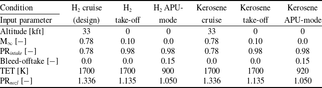
The modelled flight conditions and the corresponding input parameters are stated in Table 2. Note the variations in pressure ratio (PR) of the intake and nozzle. This is due to the difference in speed and how that affects both the intake losses and the pressure field around the tailcone and exhaust [Reference Bariş17]. The intake PR, determined using CFD by Heidebrecht et al. [Reference Heidebrecht, Barara, Bariş, van Schie, Rao and Isikveren43] and by Bari
 ${\rm{s}}$
[Reference Bariş17], is with respect to the free stream, which means that it includes the total pressure losses in the boundary layer.
Defining characteristics of the analysed conditions

Table 2 Long description
The table has six columns and seven rows, including headers. The columns are labeled as H2 cruise (design), H2 take-off, H2 APU-mode, Kerosene cruise, Kerosene take-off, and Kerosene APU-mode. The rows are labeled as Altitude, M infinity, PR intake, Bleed-offtake, TET, and PR nozzle. Row 1: Altitude, 33, 0, 0, 33, 0, 0. Row 2: M infinity, 0.78, 0.10, 0.0, 0.78, 0.10, 0.0. Row 3: PR intake, 0.78, 0.98, 0.98, 0.78, 0.98, 0.98. Row 4: Bleed-offtake, 0.0, 0.0, 0.15, 0.0, 0.0, 0.15. Row 5: TET, 1700, 1700, 900, 1700, 1700, 920. Row 6: PR nozzle, 1.336, 1.135, 1.050, 1.336, 1.135, 1.050.
The main engine parameters are the output power required, the TET and the compressor pressure ratios. These, and the more detailed input parameters, were taken from the previous design study [Reference Heidebrecht, Burger, Hoogreef, Vos, Isikveren and Rao13, Reference Rao and Yin44]. Table 3 lists the inputs used, where the bolded parameters are inputs for the design condition only, as they depend on the cycle and thus the outputs during the off-design conditions.
Component inputs for the pyCycle analyses (bold values are design-condition-only inputs)

Table 3 Long description
A table comparing component inputs for engine analyses. The table has 12 rows and 4 columns. The columns are labeled Pressure loss, Value, Pressure Ratio, and Value. The rows are labeled LPC-HPC duct, Combustor, HPT-LPT duct, LPT-PT duct, PT-nozzle duct, Combustor, HP-shaft, LP-shaft, PT-shaft, LPC, HPC, Bleed fraction, and Leakage. The values in the table are as follows: Row 1: LPC-HPC duct, 1.5, LPC, 5.8. Row 2: Combustor, 5.0, HPC, 4.5. Row 3: HPT-LPT duct, 1.0, Bleed fraction, Value. Row 4: LPT-PT duct, 1.0, Leakage, 0.005. Row 5: PT-nozzle duct, 2.0, Efficiency, Value. Row 6: Combustor, 100, Shaft speed, Value. Row 7: HP-shaft, 99.5, HP-shaft, 15000. Row 8: LP-shaft, 99.5, LP-shaft, 8000. Row 9: PT-shaft, 99.5, PT-shaft, 6000.
Analysis with kerosene as fuel was regarded as an off-design operation because the APPU engine is intended to operate on both fuels. The kerosene operating conditions were defined in terms of TET since the APPU engine is an auxiliary engine. This means that a variation in power or thrust, which the APPU can provide, is compensated for by the main engines. Although a decrease in engine power with kerosene as fuel is therefore not desirable, it is an acceptable reduction in capability for the case of insufficient LH availability
 $\textrm{LH}_2$
.
Lastly, additional inputs for the SIR cycle that are specific to the new components are required, as shown in Table 4. The choice of an SR of 0.13 is explained with a sensitivity analysis in Subsection 5.4.
Additional input parameters of the SIR APPU engine in pyCycle

Table 4 Long description
A table with two columns and ten rows. The first column lists parameters and the second column lists their corresponding values with units. The parameters include SR, E H R S G, d P H R S G k, d P H R S G sw, E condenser, d P condenser, P watertank, T watertank, P R watercompressor, η watercompressor, d F main. The values are 0.13, 0.8, 5 percent, 5 percent, 0.8, 5 percent, 2 E 5 P a, 330 K, 20, 90 percent, 2 percent respectively.
4.2 Baseline results
With the flight conditions of Table 2 and the engine parameters of Table 3, the pyCycle model is run. According to the turbomachinery efficiency determination method explained above, the design condition efficiencies are as stated in Table 5. The resulting engine performance of the baseline APPU is listed in Table 6.
Calculated component isentropic (left) and polytropic (right) efficiencies of the APPU

Table 5 Long description
A table comparing component efficiencies of an APPU. The table has five rows and four columns. The columns are labeled 'Component', 'Base isentropic efficiency', 'Cooling air fraction', 'Cooling air efficiency penalty', and 'Base politropic efficiency'. The rows are labeled with the components: LPC, HPC, HPT, LPT, and PT. Each row contains values for the respective component's efficiencies and penalties. For example, the LPC row shows values of 0.890, 0.913, and so on. The table provides a detailed comparison of the efficiencies and penalties for each component.
Baseline APPU performance results calculated with pyCycle

Table 6 Long description
The table presents performance parameters of an APPU under various conditions, including H2 cruise, H2 take-off, H2 APU mode, Kerosene cruise, Kerosene take-off, and Kerosene APU mode. It has six columns and seven rows. The columns are labeled as Condition, H2 cruise (design), H2 take-off, H2 APU mode, Kerosene cruise, Kerosene take-off, and Kerosene APU mode. The rows are labeled as Output parameter, Power [kW], SFC [kg/kWh], Win [let/s], OPR, ηthermal [%], and SFC corr. [kg/kWh]. Row 1: Output parameter, Did, N 1, Bucket, Bucket, Bucket, Bucket. Row 2: Power [kW], 2200, 5273.4, 263.0, 1935.7, 4158.3, 258.7. Row 3: SFC [kg/kWh], 0.0674, 0.0715, 0.1802, 0.1857, 0.20251, 0.49623. Row 4: Win [let/s], 3.777, 9.890, 4.254, 3.534, 8.527, 4.170. Row 5: OPR, 25.71, 20.57, 5.463, 24.44, 18.01, 5.445. Row 6: ηthermal [%], 44.5, 42.0, 16.7, 45.0, 41.3, 16.9. Row 7: SFC corr. [kg/kWh], 0.0696, 0.0738, 0.1860, , , .
Preliminary geometric design of the APPU engine core generated by Gasturb.

Lastly, the engine mass is calculated by Gasturb. The calculated mass is 502 kg, which is in good agreement with the engines in that category, and Fig. 10 shows the preliminary geometric design of the APPU. Note the PT-shaft exiting the engine through the front, contrary to what is envisioned for the APPU. The lack of architectural flexibility of Gasturb prohibits changing this configuration. This might affect the resulting engine mass, introducing uncertainty in the estimated value. However, the magnitude of this uncertainty is beyond the scope of this project as it involves a detailed geometrical design.
4.3 The effect of steam injection and recovery results
The performance of the SIR APPU is determined in a similar manner. The turbomachinery efficiencies are found to be practically equal, with slightly larger cooling air fractions as a result of the higher specific heat of the post-combustion and steam injection gases. The flight conditions are the same, except for the addition of hydrogen operation without HEs conditions. These simulate the SIR APPU with HEs that are inoperable and thus an SR of zero. Analysing these conditions gives insight into the effect of different quantities of water in the exhaust, as well as the effect of risks involved with the novel HEs. Table 7 lists the SIR APPU performance variables.
SIR APPU performance results calculated with pyCycle

Table 7 Long description
The table compares performance variables of SIR APPU under different conditions. It has 12 columns and 7 rows, including headers. The columns are Power (kW), SFC (kg/kWh), W_inlet (kg/s), OPR, η_thermal (%), W_water (g/s), rel. NOx, and SFC_corr (kg/kWh). The rows are labeled with different operational modes: H2 cruise, H2 take-off APU mode, Kerosene cruise, Kerosene take-off, Kerosene APU mode, H2 cruise HEs off, H2 take-off HEs off, and H2 APU mode HEs off. Each row lists the corresponding values for the performance variables. Notable trends include variations in power, specific fuel consumption, inlet mass flow rate, overall pressure ratio, thermal efficiency, water mass flow rate, relative NOx, and corrected specific fuel consumption across different operational modes and fuel types.
Comparison of the baseline and SIR APPU design condition results

Table 8 Long description
A table comparing baseline and SIR APPU design condition results for various parameters. The table has three columns: Parameter, Baseline cycle, SIR cycle, and Difference. Row 1: SFC [kg/kWh], 0.0674, 0.0664, 1.54 percent. Row 2: SFC $_{corr}$ [kg/kWh], 0.0696, 0.0646, 7.18 percent. Row 3: W $_{inle}$ [kg/s], 3.777, 3.637, 3.70 percent. Row 4: Relative NO $_x$ [], 1.0, 0.666, 33.4 percent. Row 5: Mass [kg], 502, 581, plus 15.7 percent. Row 6: Baseline components [kg], 502, 483, 3.70 percent. Row 7: HEs [kg], 0, 98, N.A.
Lastly, the mass of the SIR APPU needs to be determined. The slightly lower inlet mass flow rate gives a core mass of 483 kg. The highest mass flow rate through the HEs seen is 10.06 kg/s during the take-off. Thirteen per cent of this passes through the HEs, which is 1.31 kg/s, giving a total HE mass of 98.0 kg, which brings the estimated SIR APPU mass to 581 kg. Note that not all new components have been incorporated into the mass estimation yet, such as the water/steam tubing.
With the SIR APPU performance known, it can be compared to the baseline APPU performance. Performance differences are summarised in Table 8. When fuel temperature is ignored, slight improvements in SFC and SP are observed. When applying corrections due to the fuel temperature (see Section 3.4), the SFC benefit of the SIR cycle is considerably improved. The SIR cycle shows a significant reduction in NO
 $_x$
emissions, narrowly staying within the valid region of Equation (6), at the cost of a mass increase of 15.7.
4.4 Sensitivity analyses
The analyses performed use many input parameters, some of which carry significant uncertainty. To gain insight into the significance of their accuracy, sensitivity analyses are performed. Three parameters are varied: the SR, E and pressure drop (dP). Three separate sensitivity analyses are made, where in each one parameter is varied and the other two are kept constant.
The first is the splitting ratio. This sensitivity analysis determined the SR used for the main analyses, as there is an optimum. The effect of varying the SR on the SFC, SP, relative NO
 $_x$
emissions and the water mass flow rate is shown in Fig. 11. The optimal SR is found to be 0.13. At a lower SR, there is little water vapour flowing through the HEs, limiting the impact the new components can have. This is apparent from the linearly increasing flow rate of the water mass in this region. At higher SR, there is not enough cooling potential in LH fuel
 $_2$
to cool the flow to a point where most of the water vapour present is condensed and recovered. Past SR=0.20, this results in no water being condensed.
Effect of SR on the SFC, SP and relative NO
 $_{\rm{x}}$
emissions of the SIR APPU, SR between 0.01 and 0.25.

4.5 Hydrogen-kerosene differences
The next sensitivity analysis is the effectiveness of HE. The effectiveness of an HE and its pressure loss are correlated, but for simplicity and to better highlight the impact of a single parameter, they vary separately. The two HEs are given the same effectiveness, which is varied from 0.5 to 1.0. The outcome can be seen in Fig. 12. Similar effects as with the SR are observed: at low
 $E$
there is insufficient heat transfer for condensing most of the water. From about
 $E$
= 0.8 and higher, most or all of the water can be condensed, maximising the impact of the SIR cycle. The further reduction in SFC is the result of more heat being recovered in the water flow in the HRSG. However, as explained before, an effectiveness greater than 0.8 is unrealistic.
Effect of heat exchanger effectiveness on the SFC, SP and relative NO
 $_{\rm{x}}$
emissions of the SIR APPU,
 ${\rm{E}}$
between 0.5 and 1.0.

Lastly, the effect of variation on HE pressure loss is investigated. Both HEs are again given equal values, and the pressure loss is varied between zero and 10% for each HE. Figure 13 shows the results. The impact on the water mass flow rate and NO
 $_x$
emissions is insignificant, and the expected effect on SFC and SP is observed; lower pressure losses improve performance. The bumps are believed to be caused by numerical errors or instabilities.
Effect of HE pressure loss on the SFC, SP and relative NO
 $_{\rm{x}}$
emissions of the SIR APPU, dP between 0.0 and 0.1.

5.0 Discussion
A peculiarity is noticed in these results. There are large differences between the hydrogen and kerosene operating conditions. In addition, there is an oversight with a significant potential impact that has not yet been discussed. This section dives into these two aspects.
5.1 Differences between baseline and SIR engine
Table 8 compares the baseline engine cycle with the SIR version. The largest difference is a 33.4% reduction in thermal NO
 $_x$
emissions, due to steam injection, a direct outcome of Equation (6).
In addition, the recovery of heat from the combustor through the extracted water enables a 1.54% reduction of SFC. This benefit increases to 7.2% when also accounting for the fuel temperature, as H
 $_2$
is used to absorb condensation heat and carry this energy back into the combustion chamber. Since the corrected SFC for the baseline engine needs to be regarded as a worst-case scenario (see Section 3.4), it may be more appropriate to compare the corrected SFC of the SIR engine to the uncorrected baseline cycle, effectively assuming that the baseline fuel system can obtain sufficient heat from engine-external sources to heat hydrogen under standard conditions. Even under these assumptions, the SIR engine consumes 4.2% less fuel than the baseline, a considerable improvement.
The difference in engine mass and HE is 15.7% of the baseline engine mass. More fuel system components are likely required, increasing the mass penalty accordingly. However, it should be noted that the fuel system of the baseline engine would also require many components that were beyond the scope of this study, including heat exchangers. Taking the calculated mass increase at face value, the additional mass may or may not be a viable trade-off for the increased efficiency. In terms of overall aircraft mass, improved efficiency allows for a lower fuel mass H
 $_2$
and accordingly a reduced tank mass, or increases the total thrust and power contribution of the APPU engine with constant LH
 $_2$
tank size, thus reducing kerosene mass at take-off for a given mission. In both cases, the architecture change is likely only viable for longer ranges, although the current data do not permit an estimate.
During kerosene operations, the efficiency of the SIR APPU engine is similar to the baseline engine, with 2% lower in cruise but 2.5% worse at take-off, while losing up to 10% power. However, these numbers are difficult to interpret since the engine cycle and all components are sized exclusively for H
 $_2$
operations. This means that the performance with kerosene is incidental to the part of each compressor and turbine map on which kerosene operations occur, and the performance could likely be improved notably by shifting the operating point of each component in a suitable way. Despite this, the steam recovery components of the SIR engine are not effective when operating on kerosene, which means that they are mainly a source of additional pressure losses. In order to change this, considerable changes to the water recovery components would be required.
5.2 Hydrogen-kerosene differences
For both the baseline and SIR APPU, large differences can be observed between hydrogen and kerosene operation. For example, in the case of kerosene, the baseline APPU generates 12.0% less power compared to the hydrogen cruise. The same comparison for the SIR APPU gives 20.1% less power when operating on kerosene. This is the result of different specific heat capacities (
 ${C_P}$
) of the combustion products, leading to different amounts of energy to be extracted by the turbine. Hydrogen combustion creates more water than kerosene combustion, even when normalising for the heat released, leading to a higher flow
 ${C_P}$
. This can be illustrated by ‘designing’ a hydrogen and a kerosene engine.
Since the flow arrives in the combustion chamber at the same temperature and the TET is the same, an increase in temperature occurs at the same time through combustion in both the H
 $_2$
and the kerosene engines. However, due to the discrepancy in
 ${C_P}$
, a 10.0% higher specific thermal power is observed; 1.39 MW/(kg/s) in the H
 $_2$
engine and 1.26 MW/(kg/s) in the kerosene engine. Since the OPR is equal, the pressure drop and thus the temperature drop in the turbine stages are equal (neglecting differences in the specific heat ratio (
 $\gamma $
) and the amount of cooling air). This means that, due to the higher
 ${C_P}$
, more power is extracted when operating with H
 $_2$
as fuel. This effect, with a similar extent of its impact, was also observed by Mourouzidis et al. [Reference Mourouzidis, Singh, Sun, Huete, Nalianda, Nikolaidis, Sethi, Rolt, Goodger and Pilidis45], who analysed the difference between hydrogen and kerosene operations at various TET for a turbofan engine, finding a thrust discrepancy of 14.6% at TET of 1600 K.
At cruise conditions, the thermal efficiency of the SIR cycle without fuel temperature corrections is found to be equal for kerosene and H
 $_2$
operations, while the corrected SFC value corresponds to an efficiency of 46.4%, 2.7% better than the kerosene version. This illustrates the value of not only steam recovery and injection but also using available heat sources to provide H
 $_2$
at the highest feasible temperature.
6.0 Conclusion and recommendations
The purpose of this research is to quantify the impact of implementing SIR in the APPU turboshaft engine. Both cycles are modelled in pyCycle, which has been enhanced to allow analysis of the SIR cycle. The SIR cycle is found to be slightly more fuel efficient, 1.54%. NO
 $_x$
emissions are reduced by 33.4%. These improvements come at the cost of a 15.7% mass increase.
To improve the accuracy and realism of the analyses, it is recommended that any study of the engine cycle incorporate the effects of fuel temperature. Especially when comparing different cycles, this improves the validity of the comparison. This also implies that ‘simple’ baseline engine cycle designs should make accommodations for fuel conditioning if H
 $_2$
is stored in liquid form, since fuel injection at cryogenic temperatures is not advisable, and pre-heating the fuel by burning a part of it is very inefficient.
The next step in the development of the APPU engine would be to put more effort into the geometrical design and configuration of fuel systems. This improves confidence in the mass estimation and could permit the results to be used for transient and part-power analyses.
In order to improve the accuracy and confidence of the analyses and to further the development towards an SIR APPU, further research and development are recommended on multi-phase or supercritical HEs. In addition, more effort is needed to design the combustion chamber. This can allow for a more accurate estimate of the reduction in NO
 $_x$
due to steam injection, as well as a determination of the practically achievable NO
 $_x$
emissions. Lastly, to investigate the economic viability of the SIR cycle, a cost analysis should be performed.
Acknowledgement
This project has been financed by the Dutch Ministry of Economic Affairs and Climate under the TKI scheme (Grant number TKI HTSM/18.0170) along with SAFRAN TECH and the Veni grant (AES) (Grant No. 20312).


 x


 2

 2


 x

 x
 E

 x


