1 Introduction
Changes in surface roughness occur in a variety of practical applications and it is important to understand the development of the flow past the surface change. Past a change in roughness, the entire turbulent boundary layer does not immediately adapt, rather, a state of non-equilibrium exists as discussed in the review by Smits & Wood (Reference Smits and Wood1985). The term internal boundary layer is used to denote the height at which the new wall condition affects the existing boundary layer. For the flow past a rough-to-smooth (
 $\text{R}\rightarrow \text{S}$
) surface change, the flow retains characteristics of the upstream rough-wall condition above the internal layer, whereas within the internal layer the turbulence adjusts to the smooth-wall condition, see for example Antonia & Luxton (Reference Antonia and Luxton1972). Much of the past focus of the flow over a change in surface condition has been towards the characterization of the internal boundary layer development as reviewed in Savelyev & Taylor (Reference Savelyev and Taylor2005). In this study the focus is on the behaviour and characterization of the turbulence following a rough-to-smooth surface change. From a broader perspective the
 $\text{R}\rightarrow \text{S}$
surface change inherently results in an upward shift of the inner-normalized streamwise velocity profiles, which is consistent with a drag reduced flow. Therefore the behaviour and scaling of this flow has potential applicability to the control of turbulent boundary layer drag.
Over a smooth wall, the peak streamwise Reynolds normal stress occurs near the wall as a result of the viscous cycle of streaks and quasi-streamwise vortices. This peak is nominally found at
 $y^{+}\approx 15$
(where
 $y$
is the distance from the wall and the superscript
 $+$
denotes non-dimensionalisation with skin friction velocity,
 $U_{{\it\tau}}$
and kinematic viscosity,
 ${\it\nu}$
), see for example De Graaff & Eaton (Reference De Graaff and Eaton2000). Comparatively, over a rough surface and given a sufficient roughness height, the form drag associated with the roughness elements dominate over the viscous drag and the peak streamwise Reynolds normal stress often occurs in the range
 $y/{\it\delta}=0.05{-}0.2$
as discussed in the review by Jiménez (Reference Jiménez2004), where
 ${\it\delta}$
is the boundary layer thickness. Consequently, for a flow past a rough-to-smooth surface change, two distinct energetic regions are present within the boundary layer over the smooth wall, as shown by Antonia & Luxton (Reference Antonia and Luxton1972), even at a relatively low Reynolds numbers where a comparable smooth-wall boundary layer would exhibit only a single distinct energetic peak near the wall. Antonia & Luxton (Reference Antonia and Luxton1972) also demonstrated that second-order statistics such as the streamwise and wall-normal stresses were slow to adjust to the new boundary condition in the outer region. After approximately 16
 ${\it\delta}$
, the profiles of the mean flow and turbulence statistics were yet to fully relax to comparable smooth-wall equilibrium values.
Immediately following a
 $\text{R}\rightarrow \text{S}$
surface change, the skin friction is reduced below both the upstream rough-wall value and that of the smooth-wall far downstream. Existing models, for example by Elliott (Reference Elliott1958), predict this behaviour but tend to underestimate the wall shear as was shown by Chamorro & Porté-Agel (Reference Chamorro and Porté-Agel2009). It is important to note that Elliott (Reference Elliott1958) assumed that the near-wall velocity profile is in equilibrium over the downstream surface. Chamorro & Porté-Agel (Reference Chamorro and Porté-Agel2009) improved the estimation of the velocity profile downstream of a
 $\text{R}\rightarrow \text{S}$
surface change by blending the log-law for the upstream and downstream condition, and hence improved the shear stress estimate. It was found that a nonlinear blending function was required to reproduce experimental observations. Recent evidence confirms the nonlinearity of interactions between the inner and outer regions in turbulent wall-bounded flows (Ganapathisubramani et al.
Reference Ganapathisubramani, Hutchins, Monty, Chung and Marusic2012), albeit for a smooth-wall boundary layer in equilibrium.
This experimental study examines the response of the boundary layer occurring over a surface that transitions from a rough-to-smooth boundary condition. Two different rough surfaces are considered, the first is a grit-type roughness and the second is a mesh-type roughness, which provide two different inflow conditions. In addition, the mean roughness height for the mesh is approximately twice that of the grit resulting in a larger step strength for the rough-to-smooth transition. To compare the two cases we first consider the mean flow and turbulence statistics, which are common to the research of Antonia & Luxton (Reference Antonia and Luxton1972). We also examine the scaling of the resulting non-equilibrium boundary layer from the perspective of outer variable scaling, inner variable scaling and mixed scaling arguments. Regardless of the scaling, two distinct energetic regions persist following the rough-to-smooth change in the wall condition. The turbulence spectra are examined across the boundary layer to determine how the turbulent scales manifest energetically. The overarching objective of this study is to examine the interaction between the newly established near-wall region and the outer region that persists from upstream conditions.
2 Experimental arrangement
2.1 Facility
Experiments were performed in a suction-type wind tunnel at the University of Southampton. The
 $7:1$
contraction of the tunnel is followed by a working section that is 4.5 m long, with a 0.9 m
 $\times$
0.61 m cross-section, then a diffuser and fan. Measurements were performed on the turbulent boundary layer established on a 10 mm thick boundary layer plate, which spanned the 0.9 m width of the test section. The sharp leading edge of the plate was machined from aluminium to a
 $15^{\circ }$
angle, such that the measurement side of the plate was flat over the entire plate length. After the leading edge 5 interchangeable plates were fitted. The first plate was 0.5 m long while the following plate sections were 0.9 m long. Each of the smooth plates were manufactured from 1 mm thick aluminium sheet, which sandwiched an 8 mm thick aluminium honeycomb structure such that the total plate thickness was 10 mm. Plate segments were adjusted flush and a 1 mm gap between each of the plate segments was filled with wax and then shaved smooth to reduce a potential step between plates. Following the plate segments, a 0.5 m long adjustable flap was included to control the circulation around the boundary layer plate such that the leading edge stagnation point was located on the measurement side of the leading edge. The free stream velocity (
 $U_{\infty }$
) of all experiments reported was approximately
 $10~\text{m}~\text{s}^{-1}$
. Over the measurement region considered, which was between 2 and 3.5 m downstream of the leading edge, the acceleration parameter,
 $K=({\it\nu}/U_{\infty }^{2})(\text{d}U_{\infty }/\text{d}x)$
, where
 ${\it\nu}$
is the viscosity, was less than
 $2.1\times 10^{-8}$
, such that a pressure gradient effect can be assumed to be negligible (see for example Flack, Schultz & Shapiro Reference Flack, Schultz and Shapiro2005; Schultz & Flack Reference Schultz and Flack2009).
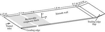
A schematic of the boundary layer plate and the coordinate system invoked is shown in figure 1. As shown, the streamwise and wall-normal coordinates are given by
 $x$
and
 $y$
, respectively, and the streamwise origin (
 $x=0$
) is from the interface of the rough and smooth walls. The instantaneous velocity in the streamwise direction is denoted by the sum of the mean and fluctuating components,
 $U+u$
. The superscript
 $^{+}$
is used throughout to denote the viscous scaling of length (
 $y^{+}=yU_{{\it\tau}}/{\it\nu}$
), velocity (
 $U^{+}=U/U_{{\it\tau}}$
) and time (
 $t^{+}=tU_{\infty }^{2}/{\it\nu}$
).
Schematic of the boundary layer plate and the coordinate system.

2.2 Roughness topologies
Two rough surfaces were considered, an abrasive grit and an extruded wire mesh, which are similar to those found in Birch & Morrison (Reference Birch and Morrison2011). The grit-type roughness consists of sheets of 16-gauge industrial open-type silicon carbide abrasive. The topology of this surface is sparse and considered isotropic and highly non-Gaussian, as is shown by Birch & Morrison (Reference Birch and Morrison2011). The mesh-type roughness is formed from an expanded aluminium sheet consisting of twisted rectangular elements, of cross-section
 $2.35\times 1.5$
mm, forming a diamond-shaped pattern. The resulting diamond shapes were elongated in the spanwise direction. These shapes are 30.5 mm wide and 11.7 mm long such that the spanwise-to-lengthwise aspect ratio is 2.6. The maximum roughness height (
 $k_{max}$
) for the grit and mesh roughness topologies are approximately 2 and 4 mm, respectively.
2.3 Constant temperature anemometry
Measurements of the flow velocity in the time domain were made using both single and two-component hot-wire anemometry. The single wire was an Auspex A55P05 boundary layer probe that had 10 mm long prongs spanned by a 3 mm long,
 $5~{\rm\mu}\text{m}$
diameter tungsten wire with a central 1.05 mm active region shouldered on either side by copper-plated sections. The resulting length-to-diameter ratio was 210, following the recommendation laid out by Ligrani & Bradshaw (Reference Ligrani and Bradshaw1987) and Hutchins et al. (Reference Hutchins, Nickels, Marusic and Chong2009). The two-component Dantec model 55P61 hot-wire probe was used to measure the streamwise and wall-normal velocity components for the purpose of calculating only the shear stress over the rough surfaces. Measurements made using the cross-wire were limited to
 $y>4$
mm, whereas the single wire could reach the wall. A StreamLine Pro CTA (constant temperature anemometer) system was used to operate the single wire, whereas the cross-wire was operated by a system developed at The University of Newcastle (see Miller, Shah & Antonia Reference Miller, Shah and Antonia1987). Data from each CTA were sampled by a 16-bit National Instruments USB-6212 BNC, A/D data acquisition card, connected to a PC at a rate of 80 kHz. Aliasing of each signal was prevented by low-pass filtering all signals below the Nyquist frequency. The hot wires were calibrated statically in the test section against a Pitot-static tube connected to a Furness FCO510 (0–200 Pa) pressure transducer over a range of velocities between
 $1.2~\text{m}~\text{s}^{-1}$
and
 $1.2U_{\infty }$
. A modified version of King’s law was fit to the calibration data, where the exponent of the velocity was included in the fit parameters (see Bruun Reference Bruun1995). Velocity data of the cross-wire signals were reduced using the look up table calibration method described by Burattini & Antonia (Reference Burattini and Antonia2005). The air temperature was monitored continuously throughout all experiments using a T-type Omega thermocouple located in the free stream and connected to an Omega CNi32 analog output meter. The CTA output signals were corrected to the reference air temperature during calibration (see Bruun Reference Bruun1995), although the ambient temperature variation remained within
 $\pm 0.7\,^{\circ }\text{C}$
. Regardless, calibrations were performed immediately before and after each experiment to linearly correct for drift. The total uncertainty of the velocity measurements were within
 $\pm 1.1$
%. Uncertainties were calculated using standard analysis methodologies, see for example Taylor (Reference Taylor1997), and include the accuracy of the reference velocity, goodness of the calibration fit and drift uncertainty.
Boundary layer profiles were acquired upstream of the
 $\text{R}\rightarrow \text{S}$
surface change at
 $x=-400,-300,-200,-100$
and
 $-50$
mm. Along the smooth wall, profiles were acquired at
 $x=10$
, 50, 100, 200, 300, 630, 805, 980, 1160 and 1320 mm. Measurement of the boundary layer profiles were automated using a Parker Automation linear traverse in conjunction with a PDX series ministep drive. For each measurement, a sufficiently long sample length (
 $T$
) between 15 000 and 19 000 boundary layer turnover times (
 $TU_{\infty }/{\it\delta}$
), where
 ${\it\delta}$
is the boundary layer thickness, was used to converge the energy occurring at the largest scales, following the recommendation of Hutchins et al. (Reference Hutchins, Nickels, Marusic and Chong2009). Each traverse typically consisted of 4 linearly spaced points in the near-wall region followed by logarithmic spacing up to 0.92–0.95
 ${\it\delta}$
and then followed again by linear spacing. The traverses contained approximately 45 measurement locations, which extended to approximately 1.3
 ${\it\delta}$
. The boundary layer thickness,
 ${\it\delta}$
, is specified at the height where 99 % of the free stream velocity was reached. Note that for the outer length scale
 ${\it\delta}$
is used, since unlike integral parameters it is independent of the shape of the profile. However, since the spacing near the edge of the boundary layer became large owing to the logarithmic measurement spacing, the uncertainty of the estimate of
 ${\it\delta}$
was within
 $\pm 3\,\%$
for all the measurements shown. For comparison, the modified Coles law of the wall/wake formulation (see Jones, Marusic & Perry Reference Jones, Marusic and Perry2001), leads to
 ${\it\delta}_{c}$
values that are always larger than
 ${\it\delta}$
, and varied between 15 to 25 %.
2.4 Preston tube
Over the smooth surface the shear stress was estimated using the Preston tube method. This method required the difference between the total pressure, determined from a tube that was open to the oncoming flow while in contact with the wall, and the static pressure,
 ${\rm\Delta}p_{p}$
. The total pressure was measured by a stainless steel tube having an outer diameter,
 $D=2.77$
mm, and an inner-to-outer diameter ratio of approximately 0.7. For the two upstream roughness cases considered, the corresponding viscous-scaled tube diameter is within
 $28<D^{+}<70$
over the smooth wall. The total pressure tube was given a minor curvature and fixed with tape at the centre of its 15 cm length to ensure that the tube opening firmly contacted the plate. The static pressure was measured from 1 mm diameter ports drilled through the surface of the plate and located 15 mm along the span from the total pressure probe to reduce any potential interference. Time-averaged measurements of
 ${\rm\Delta}p_{p}$
were made using a Furness FCO510 (0–200 Pa) pressure transducer. The shear stress was reduced using the Patel (Reference Patel1965) calibration within
 $1.5<\log _{10}({\it\tau}_{w}D^{2}/4{\it\rho}{\it\nu}^{2})<3.5$
, where
 ${\it\tau}_{w}$
is the surface shear stress,
 ${\it\rho}$
is the fluid density and
 ${\it\nu}$
is the viscosity. The variation of the wall shear stress was highest near the rough-to-smooth transition and was reflected in the streamwise resolution of measurement stations, as is shown later.
The Preston tube method of determining the skin friction has been utilized for wall shear stress measurements following a
 $\text{R}\rightarrow \text{S}$
change in surface condition (Antonia & Luxton Reference Antonia and Luxton1972; Taylor, Taylor & Coleman Reference Taylor, Taylor and Coleman1993; Loureiro et al.
Reference Loureiro, Sousa, Zotin and Silva Freire2010, for example), although it is only strictly valid for a smooth-wall boundary layer. In the recent study by Loureiro et al. (Reference Loureiro, Sousa, Zotin and Silva Freire2010) several methods to determine the wall shear were compared experimentally. It was shown that the shear stress determined by the Preston tube method agreed within 10 % of that determined from the near-wall profile. Comparatively, Taylor et al. (Reference Taylor, Taylor and Coleman1993) suggests that Preston tube measurements are accurate within 6 % of the wall shear stress following a
 $\text{R}\rightarrow \text{S}$
change in surface condition. Note that Loureiro et al. (Reference Loureiro, Sousa, Zotin and Silva Freire2010) only considered measurements within the region
 $x/{\it\delta}<1.5$
of the
 $\text{R}\rightarrow \text{S}$
surface change, where the associated uncertainly is highest as discussed by Antonia & Luxton (Reference Antonia and Luxton1972). Regardless, the aforementioned uncertainties are larger than the uncertainty of Patel’s calibration curve fit, which is within
 $\pm \text{1.5}\,\%$
(Patel Reference Patel1965). Therefore, the fiction velocity inferred from the Preston tube measurements are considered estimates that are, except very near the
 $\text{R}\rightarrow \text{S}$
surface change, useful for determining the appropriate trends.
3 Results
In this section the properties of the turbulent boundary layer following a
 $\text{R}\rightarrow \text{S}$
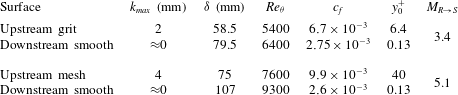
surface change for two different incoming rough-wall conditions are first examined. Next, the key variables relevant to both inner and outer scaling are examined prior to considering the boundary layers from these perspectives. The mean turbulence statistics and spectral energy distribution within the boundary layer are interpreted relative to the internal layer. The influence of the persisting outer region turbulence on the near-wall region over the smooth wall is examined and potential physical mechanisms are discussed. For reference, a summary of quantities related to the initial incoming rough-wall condition and farthest downstream measurement over the smooth surface are given in table 1.
Experimental parameters of the flow domain including the maximum roughness height (
 $k_{max}$
), momentum thickness Reynolds number (
 $Re_{{\it\theta}}$
), skin friction coefficient (
 $c_{f}$
), roughness length (
 $y_{0}$
) given by (3.2) in viscous units, and the magnitude of the surface roughness change (
 $M_{R\rightarrow S}=\ln (y_{01}/y_{02})$
).

3.1 Properties of the mean flow
Following the
 $\text{R}\rightarrow \text{S}$
surface change, the properties of the boundary layer evolve from primarily reflecting the state of the upstream rough wall to that of the downstream smooth-wall condition. For each case the variation of the shape factor,
 $H_{12}={\it\delta}^{\ast }/{\it\theta}$
, where
 ${\it\delta}^{\ast }$
and
 ${\it\theta}$
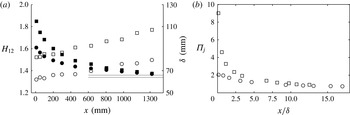
are the standard integral displacement and momentum thicknesses, respectively, are shown in figure 2(a) including the corresponding boundary layer thickness. The shape factor decreases following the
 $\text{R}\rightarrow \text{S}$
surface change. At the final measurement station, where
 $x=1.32$
m,
 $H_{12}\approx 1.38$
for each case. The corresponding momentum thickness Reynolds numbers are,
 $Re_{{\it\theta}}={\it\theta}U_{\infty }/{\it\nu}\approx 6400$
and 9300 for the grit and mesh cases, respectively, as given in table 1. From the formulation of Nagib, Chauhan & Monkewitz (Reference Nagib, Chauhan and Monkewitz2007) at these Reynolds numbers for a self-preserving smooth-wall boundary layer,
 $H_{12}\approx 1.36$
and 1.34 for the girt and mesh cases, respectively. Furthermore, the asymptotic behaviour of
 $H_{12}$
shown in figure 2(a) is evidence that the turbulent boundary layer adjusts slowly to the downstream condition, which is consistent with the results of Antonia & Luxton (Reference Antonia and Luxton1972).
(a) Development of the boundary layer shape factor,
 $H_{12}$
, and boundary layer thickness,
 ${\it\delta}$
, in the streamwise direction. Grit case shape factor, ●, and boundary layer thickness, ○; mesh case shape factor, ▪, and boundary layer thickness, ▫. Solid lines indicate
 $H_{12}=1.36$
and 1.34 for a corresponding self-preserving smooth-wall boundary layer. (b) Variation of the wake factor
 ${\it\Pi}_{j}$
for the grit, ○, and mesh, ▫, cases.

Figure 2(b) shows a comparison of the wake parameter
 ${\it\Pi}_{j}$
that was determined from the solution to
 ${\rm\Delta}(U/U_{{\it\tau}})=288{\it\Pi}_{j}^{3}/({\it\kappa}(12{\it\Pi}_{j}+1)^{2})$
, where
 ${\rm\Delta}(U/U_{{\it\tau}})$
is the maximum deviation of
 $U^{+}$
with respect to the logarithmic region (Jones et al.
Reference Jones, Marusic and Perry2001). Similar to the behaviour of the shape factor described above, the wake parameter
 ${\it\Pi}_{j}$
varies asymptotically as shown in figure 2(b). At the final measurement station for the grit case
 ${\it\Pi}_{j}\approx 0.75$
(
 $Re_{{\it\tau}}\approx 1900$
). Comparatively, for the smooth wall
 ${\it\Pi}_{j}\approx 0.71$
(
 $Re_{{\it\tau}}\approx 1430$
). For the mesh case
 ${\it\Pi}_{j}\approx 0.9$
at the farthest downstream location (
 $Re_{{\it\tau}}\approx 2500$
). Antonia & Luxton (Reference Antonia and Luxton1972) show that after approximately
 $16{\it\delta}_{o}$
, where
 ${\it\delta}_{o}$
is the incoming boundary layer thickness at the
 $\text{R}\rightarrow \text{S}$
change in surface, the boundary layer is not yet at equilibrium, again demonstrating the slow response of the boundary layer following this change in surface condition.
It is apparent from figure 2 that although the boundary layer growth rate is similar for the two cases, the flow response is significantly different, which is related to the strength of the perturbation. A common approach to quantify the strength of the perturbations due to a step change in roughness is by the logarithmic difference between the two roughness heights as discussed by Andreopoulos & Wood (Reference Andreopoulos and Wood1982), for example. This follows from the general description of the logarithmic region within the self-preserving turbulent boundary layer (smooth or rough), which can be expressed as
 $$\begin{eqnarray}\frac{U}{U_{{\it\tau}}}=\frac{1}{{\it\kappa}}\ln \left(\frac{{\it\nu}(y-d)}{U_{{\it\tau}}}\right)+B-{\rm\Delta}\frac{U}{U_{{\it\tau}}}=\frac{1}{{\it\kappa}}\ln \left(\frac{y-d}{y_{0}}\right),\end{eqnarray}$$
where
 $y$
is the wall-normal distance relative to the wall,
 $d$
is the zero-plane displacement,
 ${\it\kappa}$
is the von Kármán constant and
 $B$
is the smooth-wall additive constant. In the right portion of the above equation,
 $y_{0}$
is a roughness length that is specific to the roughness geometry. Solving (3.1) for
 $y_{0}$
yields
 $$\begin{eqnarray}y_{0}=\frac{{\it\nu}}{U_{{\it\tau}}}\exp \left[-{\it\kappa}\left(B-{\rm\Delta}\frac{U}{U_{{\it\tau}}}\right)\right].\end{eqnarray}$$
The strength of the roughness step,
 $M$
, is expressed as the logarithmic difference between two roughness heights
 $\ln (y_{01}/y_{02})$
, where
 $y_{01}/y_{02}$
is the ratio of the roughness lengths for the oncoming and downstream flow relative to the rough-to-smooth change in the surface condition (Andreopoulos & Wood Reference Andreopoulos and Wood1982). For a smooth wall, both
 $d$
and
 ${\rm\Delta}U/U_{{\it\tau}}$
are zero, which was the case in the calculation of
 $y_{02}$
from the boundary layer profile at the farthest downstream measurement location (
 $x=1300$
mm). Over the rough wall
 $U_{{\it\tau}}$
was approximately constant within experimental except for
 $x<-{\it\delta}$
at
 $x=-50$
mm for the mesh case, where the presence of the downstream condition may have influenced the boundary layer. Both
 $y_{0}$
and
 $d$
were calculated by fitting mean velocity profiles to (3.1) using the methodology of Birch & Morrison (Reference Birch and Morrison2011). The roughness length,
 $y_{01}$
, was then taken as the average value of
 $y_{0}$
over the rough surfaces between
 $x=-400$
and
 $-100$
mm. In the two cases considered in this study,
 $M_{R->S}=3.4$
for the grit surface topology to a smooth wall and
 $M_{R->S}=5.1$
for the mesh topology to a smooth wall. A larger value of
 $M$
corresponds to a stronger perturbation.
Following an abrupt
 $\text{R}\rightarrow \text{S}$
change in the wall surface the skin friction immediately decreases and then begins to recover (Antonia & Luxton Reference Antonia and Luxton1972; Mulhearn Reference Mulhearn1978; Chamorro & Porté-Agel Reference Chamorro and Porté-Agel2009) to that of a comparable smooth-wall boundary layer. Over the rough surface the friction velocity,
 $U_{{\it\tau}}$
, was estimated from the sum of the viscous and turbulent stress contributions at the total stress plateau (see for example Flack et al.
Reference Flack, Schultz and Shapiro2005; Castro Reference Castro2007). For comparison,
 $U_{{\it\tau}}$
was also calculated using the modified Clauser chart procedure (with
 ${\it\kappa}=0.41$
,
 $B=5.0$
) given by Perry & Li (Reference Perry and Li1990), which provided comparable
 $U_{{\it\tau}}$
values within 7 %. At the upstream measurement stations
 $U_{{\it\tau}}$
remained approximately constant within experimental uncertainty for
 $x=-400$
to
 $-100$
or
 $-x>{\it\delta}$
.
The skin friction coefficient,
 $c_{f}$
, is related to the friction velocity by
 $c_{f}={\it\tau}_{w}/\text{0.5}{\it\rho}U_{\infty }^{2}$
, where
 $U_{{\it\tau}}=({\it\tau}_{w}/{\it\rho})^{1/2}$
. Prior to the
 $\text{R}\rightarrow \text{S}$
surface change over the rough surfaces,
 $c_{f}\approx 6.7\times 10^{-3}$
for the grit case and
 ${\approx}9.9\times 10^{-3}$
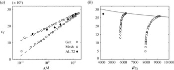
for the mesh case. Along the smooth surface the friction velocity was estimated by the Preston tube method described previously in § 2.4. The resulting variation of
 $c_{f}$
with streamwise distance (normalised by the local boundary layer thickness,
 ${\it\delta}$
) is shown in figure 3(a). Comparatively, the calculated values inferred from the Clauser chart method (
 ${\it\kappa}=0.41$
,
 $B=5.0$
) are within 4 % for
 $x/{\it\delta}>0.8$
. An additional dataset of Antonia & Luxton (Reference Antonia and Luxton1972) is included in figure 3(a) for comparison.
(a) Variation of the skin fiction coefficient,
 $c_{f}$
, with streamwise distance from the
 $\text{R}\rightarrow \text{S}$
surface change inferred from Preston tube measurements. For comparison the
 $c_{f}$
values of Antonia & Luxton (Reference Antonia and Luxton1972) are reproduced in the figure. The equation
 $c_{f}=f(M)\log (x/{\it\delta})+g$
is given by – – –. (b) Variation of the skin fiction coefficient as a function of
 $Re_{{\it\theta}}$
with the smooth-wall relationship,
 $c_{f}=2((1/{\it\kappa})\ln (Re_{{\it\theta}})+B)^{-2}$
of Österlund et al. (Reference Österlund, Johansson, Nagib and Hites2000), ——, and corresponding measurement from Antonia & Luxton (Reference Antonia and Luxton1972) at
 $x/{\it\delta}\approx 12$
.

The variation of the measured skin friction coefficient downstream of the grit and mesh roughnesses can be represented by the relationship,
 $c_{f}=f(M)\log (x/{\it\delta})+g$
, which was fit by linear least-squares regression and included in figure 3(a). The form of this equation shows that the strength of the step affects the slope of the resulting
 $c_{f}$
curve in semi-log form. As discussed earlier, the relaxation of the boundary layers appears to occur over a similar fetch (
 $x/{\it\delta}$
) for both cases. Therefore, it follows that the slope should be greater for a larger step strength given the lower skin friction achieved immediately following the rough surface. Although the step strength is not formally reported by Antonia & Luxton (Reference Antonia and Luxton1972), it is given as 5.8 by Andreopoulos & Wood (Reference Andreopoulos and Wood1982), however, this value is suspected to be erroneous as recently discussed by Jacobi & McKeon (Reference Jacobi and Mckeon2011). The expected discrepancy of
 $M_{R->S}$
is further supported by figure 3(a) since a higher expected slope is not observed. Comparing the mesh case with that considered by Antonia & Luxton (Reference Antonia and Luxton1972) suggests that these step strengths are similar.
The physical meaning of the offset (
 $g$
) is less clear, however, it is possible to speculate on its form. In one instance this value should be depend on the Reynolds number owing to the established relationship between
 $c_{f}$
and
 $Re_{{\it\theta}}$
as shown by Österlund et al. (Reference Österlund, Johansson, Nagib and Hites2000) and given by
 $c_{f}=2((1/{\it\kappa})\text{ln}(Re_{{\it\theta}})+B)^{-2}$
. The resulting variation of
 $c_{f}$
is shown in figure 3(b) as a function of
 $Re_{{\it\theta}}$
for both cases considered in this study and for the final downstream
 $c_{f}$
value of a case considered by Antonia & Luxton (Reference Antonia and Luxton1972). For the latter, we only show the final downstream location since
 $Re_{{\it\theta}}$
is given at this location. This value from Antonia & Luxton (Reference Antonia and Luxton1972) appears lower than the curve given by Österlund et al. (Reference Österlund, Johansson, Nagib and Hites2000). The source of this difference is not clear. The current data appears to collapse on the curve given by Österlund et al. (Reference Österlund, Johansson, Nagib and Hites2000) at the most downstream location. This suggests that the offset (
 $g$
) is not only related to the roughness scale of the incoming flow,
 $y_{01}$
, but must include the effect of
 $Re_{{\it\theta}}$
of the resulting smooth-wall boundary layer. Data from various other
 $\text{R}\rightarrow \text{S}$
surface change is required to confirm this observation.
3.2 Properties of the mean flow
Profiles of the turbulent boundary layer occurring past the abrupt
 $\text{R}\rightarrow \text{S}$
wall surface topology change were obtained at several locations. Measurements were made upstream of the interface at
 $x=-400$
,
 $-300$
,
 $-200$
,
 $-100$
and
 $-50$
mm. Along the smooth wall, profiles were acquired at
 $x=10$
, 50, 100, 200, 300, 630, 805, 980, 1160 and 1320 mm, however, only a selection of the results are shown for clarity. Given that the values of
 ${\it\delta}$
were different for the two cases, the resulting
 $x/{\it\delta}$
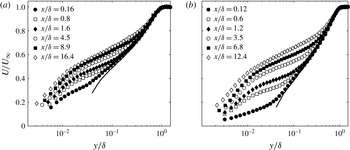
locations for the profiles do not coincide. A selection of the mean streamwise velocity profiles are plotted in semi-logarithmic format in figure 4(a) for the grit case and figure 4(b) for the mesh case and scaled in terms of the traditional outer variables,
 $U_{\infty }$
and
 ${\it\delta}$
. Downstream of the surface roughness change, a significant velocity deficit is found, which is particularly evident at
 $y/{\it\delta}<0.3$
and
 $y/{\it\delta}<0.4$
for the grit-type and mesh-type roughnesses, respectively. This height corresponds to approximately 10 times the maximum roughness height for each case and this deficit appears to persists until the final measurement location for each case.
Outer scaling of selected mean streamwise velocity profiles for the (a) grit and (b) mesh cases. The upstream rough-wall profiles are shown by —— and the data markers are for the profiles above the smooth surface.

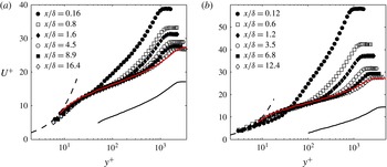
From the skin friction coefficient shown in figure 3, it is possible to consider the boundary layer from the perspective of inner scaling. Figure 5 shows the inner-scaled mean streamwise velocity for the same select cases shown in figure 4. Compared to the log-law of the wall for smooth-wall boundary layers, the well-known characteristic of the rough surface is the downward shift of the log-law, as is shown in figure 5 where the abscissa is then represented by
 $(y-d)^{+}$
for the rough-wall case. Over a smooth wall
 $d=0$
. It has been shown that following a
 $\text{R}\rightarrow \text{S}$
surface change the zero-plane displacement immediately tends to 0 or at least within
 $0.03{\it\delta}$
(Loureiro et al.
Reference Loureiro, Sousa, Zotin and Silva Freire2010). Profiles obtained past the first measurement station collapse well in the near-wall region for
 $y^{+}<30$
. However, nearest to the
 $\text{R}\rightarrow \text{S}$
surface change the inner scaled velocity exceeds the viscous condition,
 $y^{+}=U^{+}$
, which is likely an artefact of the uncertainly in the wall shear stress at this location. Regardless, the collapse of the near-wall region is remarkable. The most salient feature of figure 5 is the deviation of
 $U^{+}$
for
 $y^{+}>200$
, which is also captured by the variation of the wake parameter shown in figure 2(b). The profiles tend towards the smooth-wall case with increasing downstream distance, although note that the Reynolds number was not matched. For the smooth wall shown in figure 5(a) and in figure 5(b)
 $Re_{{\it\tau}}=2300$
, whereas
 $Re_{{\it\tau}}$
reached 1900 and 2600 for the grit and mesh cases, respectively.
Inner viscous scaling of selected mean streamwise velocity profiles for the (a) grit and (b) mesh cases. The upstream rough-wall profiles are shown by ——, where a modified abscissa is then given by
 $(y-d)^{+}$
. Smooth-wall profiles are for
 $Re_{{\it\tau}}=2300$
and are identified by —— and – – – represents
 $U^{+}=y^{+}$
.

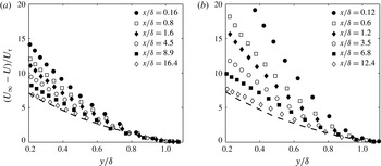
The outer region of both rough- and smooth-wall boundary layers have been shown to collapse under the velocity deficit scaling,
 $(U_{\infty }-U)/U_{{\it\tau}}=f(y/{\it\delta})$
, see for example Flack et al. (Reference Flack, Schultz and Shapiro2005). For the two cases following the
 $\text{R}\rightarrow \text{S}$
surface change, this scaling is shown in figure 6 (note that the data was only shown for
 $y>0.2{\it\delta}$
since we expect collapse in this region). At the final measurement station the inner-scaled velocity deficit approaches the smooth-wall case. Near the
 $\text{R}\rightarrow \text{S}$
surface change there is considerable deviation, which is not surprising given that the friction velocity of the upstream rough wall is higher. This confirms the inability of the outer region to scale with the local skin friction, however, this scaling will be considered later.
Inner viscous scaling of the mean deficit velocity for selected streamwise velocity profiles for the (a) grit and (b) mesh cases. The smooth-wall profile is given by – – –.

3.2.1 Identification of the internal layer
The internal layer represents the mean extent to which the different boundary conditions have influenced the flow. Methods to locate the internal boundary layer have been proposed by Antonia & Luxton (Reference Antonia and Luxton1971) and Andreopoulos & Wood (Reference Andreopoulos and Wood1982). The former employs streamwise differentiation of successive mean velocity profiles, whereas the latter relies on the dependence of the velocity gradient on the local wall shear stress. Due to the limited streamwise locations considered in this study, only the latter method is utilized. The edge of the internal layer was determined from the inflection of the mean velocity profiles in the form
 $U/U_{\infty }\propto y^{1/2}$
as explained by Antonia & Luxton (Reference Antonia and Luxton1971). Comparatively, Efros & Krogstad (Reference Efros and Krogstad2011) located the internal layer by fitting straight lines to the inner and outer distributions of the streamwise stress. However, this method is only suitable for a smooth-to-rough surface change.
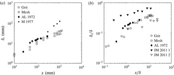
The location of the internal layer,
 ${\it\delta}_{i}$
, is shown in dimensional and non-dimensional form in figure 7. Often a simple power law is used to describe the growth of the internal boundary layer, see for example Antonia & Luxton (Reference Antonia and Luxton1972), Mulhearn (Reference Mulhearn1978), and Jacobi & McKeon (Reference Jacobi and Mckeon2011). In dimensional form Antonia & Luxton (Reference Antonia and Luxton1972) report
 ${\it\delta}_{i}\propto x^{0.43}$
whereas Mulhearn (Reference Mulhearn1978) report
 ${\it\delta}_{i}\propto x^{0.8}$
. Although Mulhearn (Reference Mulhearn1978) did not explicitly state the boundary layer thickness, the boundary layer thickness was deduced from the mean velocity profiles such that the data presented were contained within
 $x/{\it\delta}<1$
, whereas Antonia & Luxton (Reference Antonia and Luxton1972) include a range of data form
 $0.7<x/{\it\delta}<3.8$
to fit a power law. For an impulsive roughness, Jacobi & McKeon (Reference Jacobi and Mckeon2011) found that
 ${\it\delta}_{i}/{\it\delta}\propto x^{0.2}$
provided a reasonable approximation for both internal layers. However, Jacobi & McKeon (Reference Jacobi and Mckeon2011) note that two distinct internal layer growth rates may be observed based on the proximity from the step change. As reviewed by Savelyev & Taylor (Reference Savelyev and Taylor2005), there have been numerous attempts to model the location of the internal boundary layer following a step change in roughness with various levels of success. For the two cases considered in the present study, it appears that the internal layers exhibit similar behaviour when plotted non-dimensionally. Furthermore, the present results suggest two distinct regions of internal layer growth about the streamwise location of
 $x/{\it\delta}=1.5$
, however, we do not attempt to model the internal layer. As shown in figure 7(b) the evolution of the internal layer appears similar to previously reported results.
Location of the internal layer in (a) dimensional and (b) non-dimensional form. Data from the present study are included with results from Mulhearn (Reference Mulhearn1978) (M 1977), Antonia & Luxton (Reference Antonia and Luxton1972) (AL 1972) and Jacobi & McKeon (Reference Jacobi and Mckeon2011) (JM 2011 1 and 2), for comparison.

3.3 Turbulence statistics
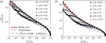
It was recently shown by Alfredsson, Örlü & Segalini (Reference Alfredsson, Örlü and Segalini2012) that starting within the logarithmic region and across a significant portion of the outer wake, the turbulence intensity (
 $\sqrt{\overline{u^{2}}}/U$
) decreases linearly with
 $U/U_{\infty }$
, viz.
 $\sqrt{\overline{u^{2}}}/U=0.286-0.255U/U_{\infty }$
for a smooth-wall boundary layer. This relationship also appears to be independent of the Reynolds number (Alfredsson et al.
Reference Alfredsson, Örlü and Segalini2012). In comparison, for a rough-wall turbulent boundary layer Castro (Reference Castro2013) showed that the slope of the linear region was greater, which confirmed the significance of wake strength suggested by Alfredsson et al. (Reference Alfredsson, Örlü and Segalini2012). The aforementioned plotting method is shown in figure 8 for the cases pertaining to the
 $\text{R}\rightarrow \text{S}$
surface change, where only data above
 $U/U_{\infty }>0.3$
are shown for demonstration. Given the robustness of the linear region slope observed by Alfredsson et al. (Reference Alfredsson, Örlü and Segalini2012), the departure from the linear region for
 $0.6<U/U_{\infty }<0.9$
shown in figure 8 can be interpreted as the effect of the persisting rough-wall boundary layer characteristics in this region of the flow. This is confirmed by examining the location of the internal boundary layer, which resides within this region as is shown in figure 8. The shaded region is used to highlight the envelope between the near-wall flow developing over the smooth wall and the portion of the flow containing the characteristic upstream rough-wall boundary layer behaviour. Within the shaded envelope region the flow exhibits a transitional behaviour owing to the competing effect between the smooth-wall condition developing away from the wall (left edge of the shaded region) and the persisting rough-wall turbulence (right edge of the shaded region). The diagnostic plot then represents a novel method to determine the location of the internal layer without relying on streamwise differentiation or intersecting curve fits.
The streamwise turbulence intensity,
 $\sqrt{\overline{u^{2}}}/U$
, with respect to the normalized mean velocity,
 $U/U_{\infty }$
, for the (a) grit and (b) mesh cases. The linear equation of Alfredsson et al. (Reference Alfredsson, Örlü and Segalini2012) for a smooth-wall turbulent boundary layer is shown by — ⋅ —, whereas the upstream rough-wall profile is shown by ——. The internal boundary layer is identified by – – – and the approximate region between the smooth- and rough-wall behaviour is shaded.

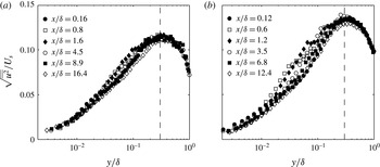
A method to scale the streamwise stress based on the mean velocity gradient was proposed by Jacobi & McKeon (Reference Jacobi and Mckeon2011), viz.
 $U_{s}=\sqrt{(U_{\infty }{\it\delta}\partial U/\partial y)}$
, to collapse the perturbed boundary layer. The scaling is applied to the current grit and mesh cases as shown in figure 9. Although the data appears to approximately collapse in the regions where
 $y/{\it\delta}<0.02$
or
 $y/{\it\delta}>0.4$
, between these regions there is a greater range of variation. Recall that the diagnostic plot, shown in figure 8, demonstrates a transitional region between the apparent smooth- and rough-wall characteristics in the outer region. This previous observation supports the interpretation that variation of
 $\sqrt{\overline{u^{2}}}/U_{s}$
within the region
 $y/{\it\delta}<0.02$
and
 $y/{\it\delta}>0.4$
occurs as a result of the development of the internal boundary layer since the envelope identified in figure 8 overlaps these locations. Additionally, the peak magnitude of
 $\sqrt{\overline{u^{2}}}/U_{s}$
for the grit and mesh cases vary significantly. This suggests that this scaling might be suitable for comparing several streamwise locations in one flow, but, might not be suitable for comparisons across different flows.
The root-mean-square of the streamwise turbulence for the (a) grit and (b) mesh cases following the
 $\text{R}\rightarrow \text{S}$
surface changes normalized by the velocity scale based on the local mean velocity gradient.

Comparatively, the data of Jacobi & McKeon (Reference Jacobi and Mckeon2011) appear to effectively collapse under this scaling, however, this may be an artefact of the relatively low step strength of the roughness impulse considered (
 ${\approx}1.7$
). Similarly, as was reproduced and scaled by Jacobi & McKeon (Reference Jacobi and Mckeon2011), albeit with additional uncertainty, greater variation was observed for the impulse cases of Andreopoulos & Wood (Reference Andreopoulos and Wood1982) having higher step strengths. Therefore, we seek alternative methods to examine and interpret the scaling of the boundary layer.
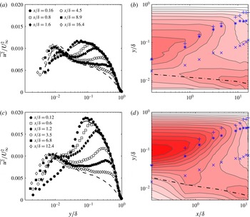
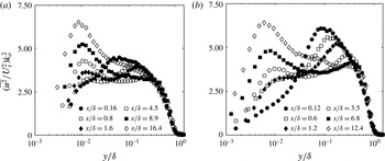
Turbulence statistics of the streamwise velocity component are shown in figure 10. Successive profiles of
 $\overline{u^{2}}/U_{\infty }^{2}$
shown in figure 10(a,c) demonstrate two distinct energetic regions over the smooth wall, downstream of the
 $\text{R}\rightarrow \text{S}$
surface change. Comparing these profiles with the flow occurring over the rough surface, it is clear that the energetic region above
 $y/{\it\delta}\approx 0.05$
is an artefact of the turbulence produced over the rough wall. The location of this region is consistent with the behaviour of fully rough, rough-wall boundary layers, where a corresponding peak is typically found between
 $y/{\it\delta}=0.05{-}0.2$
, as discussed by Jiménez (Reference Jiménez2004). Over the smooth surface, this hump both decreases in magnitude and appears to moves away from the wall with downstream fetch from the
 $\text{R}\rightarrow \text{S}$
interface as shown by the contours in figure 10(b,d). The location of the internal boundary layer and the extent of the envelope identified in figure 8 are included in figure 10(b,d). Within this region, the flow exhibits mixed characteristics of a smooth- and rough-wall turbulent boundary layer.
Outer-scaled selected profiles of
 $\overline{u^{2}}/U_{\infty }^{2}$
for the (a) grit and (c) mesh cases. The smooth-wall case is given by – – –, whereas the upstream rough-wall case is given by ——. Corresponding contours of
 $\overline{u^{2}}/U_{\infty }^{2}$
are shown to the right in (b) and (d) where the internal boundary layer is marked by
 $\ast$
while the extent of the envelope from figure 8 is identified by
 $\times$
and
 $+$
, respectively. The location where
 $y^{+}=15$
is shown by — ⋅ —. The linear colour map of
 $\overline{u^{2}}/U_{\infty }^{2}$
varies from white to red over a range from 0 to 0.02.

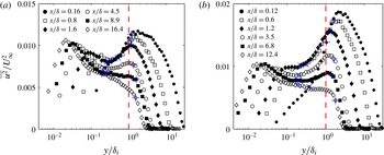
By scaling the wall-normal coordinate by the height of the internal boundary layer (
 ${\it\delta}_{i}$
) it is clear that the energetic region associated with upstream flow condition resides above
 ${\it\delta}_{i}$
as shown in figure 11. For
 $x/{\it\delta}<1$
the location of peak
 $\overline{u^{2}}/U_{\infty }^{2}$
in the outer region remains at the same position as that of the rough wall as it is yet to experience the influence of the new wall condition. Considering the first two profiles that are closest to the
 $\text{R}\rightarrow \text{S}$
interface (
 $x/{\it\delta}<1$
), the region of influence of the internal layer does not extend to the outer region peak and therefore does not modify the location of this peak. However, for
 $x/{\it\delta}>1$
, the location of the outer region peak is fixed at approximately
 $y/{\it\delta}_{i}=1.2$
. This behaviour is also displayed in figure 10(b,d) where, for
 $x/{\it\delta}>1$
, it is evident that the influence of the internal boundary layer reaches the outer region peak location, resulting in the scaling of the peak location with the internal boundary layer thickness. This suggests that the growth of the internal layer dictates the outer peak location regardless of the incoming conditions, although the growth of internal layer itself depends on the surface conditions of the oncoming flow.
Outer-scaled selected profiles of
 $\overline{u^{2}}/U_{\infty }^{2}$
for the (a) grit and (b) mesh cases where the wall-normal location
 $y$
is scaled by the internal boundary layer thickness,
 ${\it\delta}_{i}$
. The location
 $y/{\it\delta}_{i}=1$
is identified by – – –. The lower and upper extent of the envelope region shown in figure 8 is identified by
 $\times$
and
 $+$
, respectively.

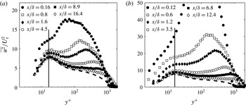
In the near-wall region an energetic site in the streamwise normal stress develops as shown in figures 10 and 11. As the near-wall cycle above the smooth surface is established, the presence of a distinct peak appears to be masked by the existing high turbulence. For example, at the first measurement location
 $\text{d}(\overline{u^{2}/U_{\infty }})/\text{d}(y/{\it\delta})$
remains positive prior to the peak in the energetic region associated with the upstream turbulence. Farther downstream, at
 $x/{\it\delta}\geqslant 0.8$
and
 $x/{\it\delta}>1.2$
for the grit and mesh cases, the inner region peak becomes well defined such that there is a sign change in
 $\text{d}(\overline{u^{2}/U_{\infty }})/\text{d}(y/{\it\delta})$
past
 $y^{+}\approx 15$
as shown in figure 10. By scaling the streamwise normal stress by the local friction velocity,
 $\overline{u^{2}}/U_{{\it\tau}}^{2}$
, the wall-normal location of the inner peak collapses as shown in figure 12. The location of the peak value of
 $\overline{u^{2}}/U_{{\it\tau}}^{2}$
in the near-wall region resides at approximately
 $y^{+}=15$
, which is also evident from the overlaid location on the contours in figure 10. This location is consistent with the inner peak typically found between
 $y^{+}\approx 12{-}16$
as shown by Fernholz & Finley (Reference Fernholz and Finley1996), for an equilibrium smooth-wall boundary layer.
Inner viscous scaling of selected profiles of
 $\overline{u^{2}}/U_{{\it\tau}}^{2}$
for the (a) grit and (b) mesh cases. The vertical —— represents
 $y^{+}\approx 15$
and – – – shows a completely smooth surface result.

The behaviour of the near-wall inner-scaled peak past the
 $\text{R}\rightarrow \text{S}$
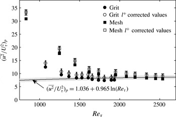
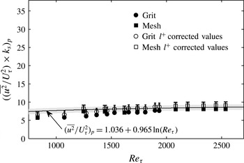
change in surface roughness, however, is not comparable to an equilibrium smooth-wall boundary layer. As shown in figure 12 the maximum value of the near-wall inner-scaled peak appears to decrease with downstream fetch. Marusic & Kunkel (Reference Marusic and Kunkel2003) showed that the maximum value of the inner-scaled near-wall peak increases with
 $Re_{{\it\tau}}$
for the smooth flat plate turbulent boundary. Hutchins & Marusic (Reference Hutchins and Marusic2007a
) describe the magnitude of the inner peak by an empirical relationship,
 $(\overline{u^{2}}/U_{{\it\tau}}^{2})_{peak}=1.036+0.965\ln (Re_{{\it\tau}})$
. Past the
 $\text{R}\rightarrow \text{S}$
change in surface roughness, both the shear stress and boundary layer thickness increase (see figures 3 and 2). This implies an increase in
 $Re_{{\it\tau}}$
and therefore an increase in
 $(\overline{u^{2}}/U_{{\it\tau}}^{2})_{peak}$
, however, the inner-scaled near-wall peak of the streamwise stress decreases immediately following the
 $\text{R}\rightarrow \text{S}$
interface as shown in figure 13(a). Within this figure the empirical relationship of Hutchins & Marusic (Reference Hutchins and Marusic2007a
) is reproduced with a shaded grey region that represents the observed scatter about this trend from the data shown by Hutchins & Marusic (Reference Hutchins and Marusic2007a
). Sufficiently far downstream the near-wall
 $(y^{+}\approx 15)$
peak value for the grit case appears to the track the empirical relationship of Hutchins & Marusic (Reference Hutchins and Marusic2007a
). For the girt case this is observed in figure 13(a) past
 $x/{\it\delta}>13$
, corresponding to the final three measurement locations, whereas the peak value appears to still be decreasing for the mesh case at the final measurement location. This is likely related to the difference in the extent of
 $x/{\it\delta}$
captured for these cases since the mesh case only reaches
 $x/{\it\delta}\approx 12.4$
due to the thicker boundary layer and fixed extent of the measurement domain. Included in figure 13 are the
 $l^{+}$
corrected values that were determined using the relationship established by Hutchins et al. (Reference Hutchins, Nickels, Marusic and Chong2009), in addition to error bars that represent a
 $\pm 10\,\%$
uncertainty on the measured
 $c_{f}$
values, which shows that the observed trends are not due to measurement uncertainty. This clearly suggests that the near-wall peak is under the influence of the outer region, which is different for the two different incoming conditions.
Variation of the inner peak magnitude with Reynolds number for the grit and mesh cases. The solid line represents the empirical relationship of Hutchins & Marusic (Reference Hutchins and Marusic2007a
) and the grey shaded region represents scatter about this fit. Open symbols show the
 $l^{+}$
corrected values and error bars represent a 10 % uncertainty in
 $c_{f}$
.

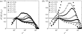
An alternative mixed scaling was proposed by De Graaff & Eaton (Reference De Graaff and Eaton2000), which appeared to improve the collapse the inner peak magnitude of
 $\overline{u^{2}}$
over a wide Reynolds number range for a smooth-wall boundary layer. The rationale for this scaling was based on Townsend’s proposition that turbulent motion in the near-wall region consists of the superposition of active shear stress producing motions that scale on inner variables and larger scales from the outer region that scale on outer variables. As is shown in figure 14, the magnitude of the near-wall peak does not completely collapse for the cases considered in this study, particularly near the
 $\text{R}\rightarrow \text{S}$
surface change, and the discrepancy is higher for the mesh case, which exhibits a higher level of distortion. However, the collapse is comparatively improved with respect to solely outer or inner scaling as shown in figures 10 and 12. For the grit case shown in figure 14(a), the collapse is remarkably near 0.3 (except for the first measurement location), which is similar for flat plate smooth-wall boundary layers (De Graaff & Eaton Reference De Graaff and Eaton2000). For the mesh case the inner peak tends toward 0.3 and appears to reach this value as the inner peak becomes well defined or the magnitude of the outer region peak reaches similar levels observed in the grit case.
Mixed scaling of selected profiles of
 $\overline{u^{2}}/(U_{{\it\tau}}U_{\infty })$
for the (a) grit and (b) mesh cases. The vertical —— represents
 $y^{+}\approx 15$
, and the horizontal —— is shown at
 $\overline{u^{2}}/(U_{{\it\tau}}U_{\infty })=0.3$
. The – – – shows a completely smooth surface result.

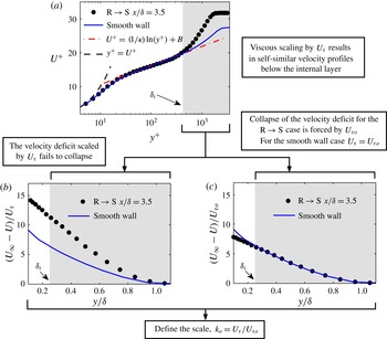
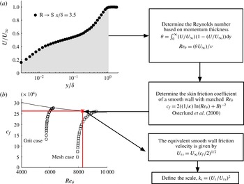
Procedure followed to determine the apparent friction velocity,
 $U_{{\it\tau}o}$
, required to force collapse of the mean velocity deficit above the internal layer. The example data is from the mesh case at
 $x/{\it\delta}=3.5$
. This procedure was repeated for each measurement station following the
 $\text{R}\rightarrow \text{S}$
surface change.

The previous mixed scaling method of De Graaff & Eaton (Reference De Graaff and Eaton2000) suggests that the scaling of the inner peak magnitude may collapse with an appropriate velocity scale associated with the outer region. However, the velocity scale associated with the outer region should reflect the recovery of the mean velocity following the
 $\text{R}\rightarrow \text{S}$
surface change. Obviously, the free stream velocity does not change with downstream distance and therefore is not the appropriate scale for this. At a first glance, the local velocity at
 ${\it\delta}_{i}$
, or at the location of the peak energy in the outer region compared to the smooth wall may appear appropriate. We also considered the outer velocity scale of Zagarola & Smits (Reference Zagarola and Smits1998) (
 $U_{\infty }{\it\delta}^{\ast }/{\it\delta}$
), which was found to collapse the outer region above the internal boundary layer. However, further analysis (not shown here for brevity) indicated that these choices do not really collapse the near-wall peak. Therefore, an alternative velocity scale is proposed where this new scale is based on forcing outer layer similarity on the mean velocity deficit.
Figure 15 shows a schematic representation of the procedure followed to determine a scale associated with the outer region of the boundary layer. As shown in this figure and previously in figure 6, the scaled velocity deficit
 $((U_{\infty }-U)/U_{{\it\tau}})$
fails to collapse downstream of the
 $\text{R}\rightarrow \text{S}$
surface change. A new velocity scale denoted as
 $U_{{\it\tau}o}$
is defined, where the subscript ‘o’ identifies this scale as the apparent skin friction velocity necessary to force similarity of the velocity deficit in the outer region above the internal layer. This new definition is motivated by the fact that outside the internal boundary layer, the flow should retain some aspects of a canonical rough-wall boundary layer as evidenced in figure 8. If we hypothesise that flow in question should exhibit outer layer similarity in the mean flow outside the internal boundary layer, then the wall conditions to enforce this similarity hypothesis cannot be given by the local friction velocity. This is because
 $U_{{\it\tau}}$
is determined by the growth of the internal layer and therefore
 $U_{{\it\tau}}$
is not an adequate scaling parameter for the entire boundary layer. At the same time, the wall conditions cannot be the
 $U_{{\it\tau}}$
of incoming flow as the ‘new’ turbulent structures that emerge from the smooth wall will alter the features of the flow even in the region outside the internal layer. Therefore, there should be an ‘equivalent’ rough wall that can capture the overall history effects of the flow. Unfortunately, it is difficult obtain a theoretical formulation for this new ‘history’ scale. Therefore, we carry out a minimisation procedure to determine it. Practically, at each measurement location downstream of the
 $\text{R}\rightarrow \text{S}$
surface change, the following objective function
 $\mathscr{J}$
is minimized to enforce outer layer similarity in the mean profile,
 $$\begin{eqnarray}\mathscr{J}=\int _{max[y/{\it\delta}_{i},0.3y/{\it\delta}]}^{1}\left[\left|\frac{U_{\infty }-U(y/{\it\delta})}{U_{{\it\tau}o}}-\left[\frac{U_{\infty }-U(y/{\it\delta})}{U_{{\it\tau}}}\right]_{smooth}\right|\right]\text{d}\left(\frac{y}{{\it\delta}}\right).\end{eqnarray}$$
This shows that at each measurement location the value of
 $U_{{\it\tau}o}$
was determined such that the outer region of the mean velocity deficit is forced to collapse with the smooth-wall case as demonstrated in figure 15. Sufficiently far downstream it is expected that
 $U_{{\it\tau}o}\rightarrow U_{{\it\tau}}$
. Upstream of this location,
 $U_{{\it\tau}o}>U_{{\it\tau}}$
, where
 $U_{{\it\tau}}$
is the friction velocity determined from the Preston tube measurements.
It is very important to note that this new ‘history’ scale is only obtained in the mean flow. There is no information included about the variance or the spectral energy content when deriving this scale. Therefore, the efficacy of this new scale on variance and/or spectra is a physical result and is not an artefact of the process used to derive it.
The new outer scale,
 $U_{{\it\tau}o}$
, is first considered with respect to the normalization of the streamwise normal stress,
 $\overline{uu}$
. Unlike the outer scaling by the free stream velocity shown in figure 10, scaling
 $\overline{uu}$
by
 $U_{{\it\tau}o}^{2}$
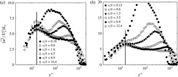
results in the collapse of the
 $\overline{uu}$
past the internal boundary location, or for
 $y/{\it\delta}>0.3$
, as shown in figure 16. This suggests that even for flows over a step change in roughness, ‘presence’ of outer layer similarity in the mean flow (in this case, this presence is forced by the choice of
 $U_{{\it\tau}o}$
) results in collapse of turbulence quantities in the outer region. The collapse of the outer region for this scaling parallels the observation made earlier from figure 9 where the streamwise turbulent fluctuations were scaled by the mean velocity gradient, again confirming the similarity of the outer region given an appropriate outer scale. However, given that this scale is purely associated with the flow above the internal boundary layer, it is does not collapse the inner peak magnitude as may be inferred from the near-wall energetic site shown in figure 16 for
 $y/{\it\delta}<0.02$
. This is to be expected because the near-wall peak should really only depend on the characteristics of the new internal boundary layer.
Outer-scaled profiles of
 $\overline{u^{2}}$
by
 $U_{{\it\tau}o}^{2}$
for the (a) grit and (b) mesh cases. Note that
 $k_{o}=U_{{\it\tau}}/U_{{\it\tau}o}$
as defined in figure 15.

The new internal boundary layer, however, is under the effect of an external boundary layer. Analogous to a high Reynolds number smooth-wall boundary layer, the near-wall peak does not just depend on the local skin friction but also on an outer velocity scale that represents the energetic motions of the outer region. Toward reconciling the near-wall peak streamwise normal stress, consider a mixed scale based on a contribution of the near-wall and outer regions,
 $U_{{\it\tau}}U_{{\it\tau}o}$
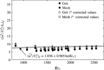
. This new scaling is essentially a geometric mean of the local skin friction and the skin friction ‘perceived’ by the outer region of the flow. The resulting mixed scale profiles are shown in figure 17. Note that the upper limit of both ordinates in figure 17 are reduced compared to those shown in figure 12. From figure 17 it is evident that the variation of the near-wall peak magnitude is substantially reduced. This is clearly shown by examining the maximum value of the inner peak scaled by
 $k_{o}=U_{{\it\tau}}/U_{{\it\tau}o}$
, which is shown in figure 18. The variance about the smooth-wall trend of the inner peak maximum value described by Hutchins & Marusic (Reference Hutchins and Marusic2007a
) is considerably reduced past the
 $\text{R}\rightarrow \text{S}$
surface change by the mixed scaling. This shows that a combination of near-wall skin friction and outer region skin friction is required to reproduce the behaviour exhibited by a canonical smooth-wall boundary layer at comparable values of
 $Re_{{\it\tau}}$
. This also suggests that the near-wall peak in the present flow is established under the influence of an energetic outer region whose characteristic velocity is a ‘perceived’ skin friction that enforces outer layer similarity.
Profiles of the mixed scaling of
 $\overline{u^{2}}$
for the (a) grit and (b) mesh cases where
 $k_{o}=U_{{\it\tau}}/U_{{\it\tau}o}$
. Inner scaling of the wall-normal coordinate is by the wall local friction velocity,
 $U_{{\it\tau}}$
. The approximate location of the inner peak (
 $y^{+}=15$
) is shown by ——.

Variation of the inner peak magnitude, scaled by
 $k_{o}$
, with Reynolds number for the grit and mesh cases. Note that the limits of the plot correspond with figure 13. The solid line represents the empirical relationship of Hutchins & Marusic (Reference Hutchins and Marusic2007a
) and the grey shaded region represents scatter about this fit. Open symbols show the
 $l^{+}$
corrected values and error bars represent a 10 % uncertainty in
 $c_{f}$
.

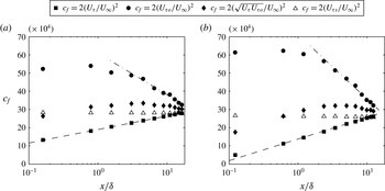
Finally, the streamwise evolution of the velocity scales can be examined by considering the skin friction coefficients based on
 $U_{{\it\tau}}$
,
 $U_{{\it\tau}o}$
, and
 $\sqrt{U_{{\it\tau}}U_{{\it\tau}o}}$
as shown in figure 19. Note that the skin friction coefficient for a comparable smooth surface
 $U_{{\it\tau}s}$
is included, which was determined from
 $Re_{{\it\theta}}$
and the empirical
 $c_{f}$
relationship given by Österlund et al. (Reference Österlund, Johansson, Nagib and Hites2000) (see appendix A). The skin friction coefficient for a smooth surface is approximately constant (
 $\pm 1.5\,\%$
) over the range of Reynolds numbers considered.
The first thing to note is that the all values of
 $U_{{\it\tau}o}$
are less than the value of
 $U_{{\it\tau}}$
of the upstream rough wall. This decrease in representative velocity scale suggests that the change in surface roughness is felt across the entire layer almost immediately. Once this ‘shock’ is felt, the subsequent response of
 $U_{{\it\tau}o}$
, and therefore the outer region, is delayed. For substantial downstream distances (say up to
 $2{\it\delta}$
), the value of
 $U_{{\it\tau}o}$
remains a constant. This is primarily because the growth of the internal boundary layer is gradual. This is consistent with previous observations of the streamwise Reynolds stress, which shows that the newly established near-wall condition is yet to interact with the outer region of the flow as shown in figure 10. For
 $x/{\it\delta}>2$
the decay of
 $c_{f}$
based on
 $U_{{\it\tau}o}$
can be captured by an equation of the form
 $c_{f}=f(M)\log (x/{\it\delta})+g$
, which has a form that is similar to the one used to describe
 $c_{f}$
based on
 $U_{{\it\tau}}$
, albeit with very different slopes and intercepts. The delayed recovery of the outer region, in contrast with the fast response of the near-wall region, leads to the variation of
 $c_{f}$
based on
 $\sqrt{U_{{\it\tau}}U_{{\it\tau}o}}$
. Furthermore, the mixed scale
 $c_{f}$
is yet to converge to the smooth wall
 $c_{f}$
trend at the final measurement location, whereas the inner peak magnitude appeared to coincide with the smooth-wall trend based on inner scaling alone, as shown in figure 13. Therefore, the slow response of the outer region appears to cause the inner peak magnitude to fall below the smooth-wall trend.
Variation of the skin fiction coefficient,
 $c_{f}$
, with streamwise distance from the
 $\text{R}\rightarrow \text{S}$
surface change for the (a) grit and (b) mesh cases. The
 $c_{f}$
values shown are for
 $U_{{\it\tau}}$
inferred from Preston tube measurements, the forced collapse of the velocity deficit,
 $U_{{\it\tau}o}$
, the mixed scaling,
 $(U_{{\it\tau}}U_{{\it\tau}o})^{1/2}$
, and the equivalent smooth wall,
 $U_{{\it\tau}s}$
. The equation of the form
 $c_{f}=f(M)\log (x/{\it\delta})+g$
is given by – – – and — ⋅ —.

3.4 Properties of the turbulent spectra
Statistics of the streamwise velocity fluctuations (
 $u$
) represent the combined influence caused over all flow scales. The spectra of the streamwise fluctuations,
 ${\it\phi}_{uu}$
, is examined to investigate the scales of motion within the turbulent boundary layer following the
 $\text{R}\rightarrow \text{S}$
wall surface change. In addition to the mean statistics reported previously, the spectra offers information on how the near-wall and outer regions of the boundary layer manifest energetically. The local convective velocity is employed using Taylor’s hypothesis to express the temporal spectra as a function of streamwise wavenumber,
 $k_{x}=2{\rm\pi}f/U$
, and wavelength,
 ${\it\lambda}_{x}=2{\it\pi}/k_{x}$
. Spectra at each wall-normal location were premultiplied by the wavenumber,
 $k_{x}$
.
The variation of the premultiplied spectrogram of
 $k_{x}{\it\phi}_{uu}/U_{{\it\tau}}^{2}$
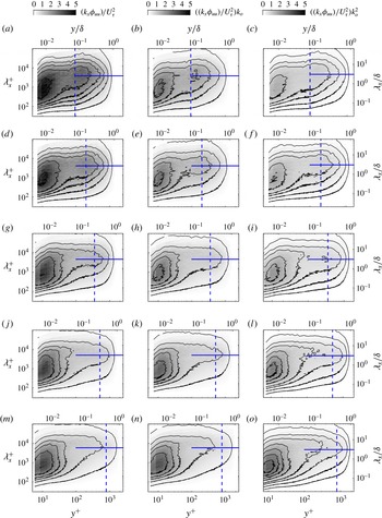
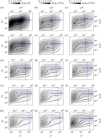
for the grit and mesh cases are shown along the left column in figures 20 and 21, respectively. The top row is spectra just downstream of the step change in roughness and subsequent rows show the data for different downstream distances. The downstream location is specified within the figure. It can be seen that for both mesh and grit cases, there is substantial energy in the outer region at large scales (approximately 3–
 $5{\it\delta}$
). The corresponding energy level is higher for the mesh case compared to the grit cases (note that the colour scale is different for the two figures). This is consistent with the fact that the mesh is a stronger roughness compared to the grit and therefore there is substantially more energy in the outer region for the mesh case. It can also be seen in the figures that for both cases, the location of energy concentration in the outer region is just at the outer edge of the internal boundary layer immediately downstream of the step change.
As the flow progresses downstream, the energy contained in the outer region appears to decrease. This is primarily because the momentum flux due to the roughness is now reduced and the outer region is ‘shielded’ by the internal boundary layer. The energy contained in this outer region diffuses and by
 $x/{\it\delta}>10$
, most of the energy is lost. At the most downstream location, the outer region resembles the outer region of a smooth-wall boundary layer. It must be noted that the recovery to smooth-wall state is not fully complete. Further measurements are necessary to confirm the distance at which complete spectral recovery will be attained.
The spectra (left column) immediately downstream of the step change also shows that the near-wall spectral peak is also stronger for the mesh case compared to the grit case. This is consistent with the variance results in the previous section. The spectra shows that the increased variance is due to a stronger near-wall cycle with the peak energy at
 ${\it\lambda}^{+}\approx 1000$
(and surrounding wavelengths). This near-wall peak appears to decrease dramatically with increasing downstream distance. This decrease appears to be stronger for the mesh case compared to the grit case indicating that the behaviour of the energetic motions in the outer region (i.e. the trends in outer spectral peak) should have role in the behaviour of the near-wall peak.
The fact that the near wall as well as the outer spectral peaks possess different strengths when scaled with
 $U_{{\it\tau}}$
suggests that different velocity scales should be examined to account for the trends exhibited. Just as in the variance, the efficacy of ‘perceived’ outer scale and a mixed scale to capture the trends in the spectra are examined. The right column of figures 20 and 21 shows the premultiplied spectrogram normalised by
 $U_{{\it\tau}o}$
while the middle column of both figures show the spectra with mixed scaling (
 $U_{{\it\tau}}U_{{\it\tau}o}$
, which is the geometric mean of the local inner scale and ‘new’ outer scale of the flow).
Variation of the premultiplied spectra for the grit case following the rough-to-smooth surface change. The premultiplied spectra is normalized by
 $U_{{\it\tau}}^{2}$
on the left and to the right the mixed (
 $k_{o}$
) and outer (
 $k_{o}^{2}$
) scalings are shown, respectively. The normalization of
 ${\it\lambda}_{x}$
and
 $y$
use the friction velocity
 $U_{{\it\tau}}$
. The location of the internal boundary layer is given by – – – and
 ${\it\lambda}_{x}=3{\it\delta}$
is shown by ——. (a–c)
 $x/{\it\delta}=0.8$
, (d–f)
 $x/{\it\delta}=1.6$
, (g–i)
 $x/{\it\delta}=4.5$
, (j–l)
 $x/{\it\delta}=8.9$
, (m–o)
 $x/{\it\delta}=16.9$
.

Variation of the premultiplied spectra for the mesh case following the rough-to-smooth change in surface. The premultiplied spectra is normalized by
 $U_{{\it\tau}}^{2}$
on the left and to the right the mixed (
 $k_{o}$
) and equivalent smooth wall (
 $k_{s}$
) scalings are shown. The normalization of
 ${\it\lambda}_{x}$
and
 $y$
use the friction velocity
 $U_{{\it\tau}}$
. The location of the internal boundary layer is indicated by – – – and
 ${\it\lambda}_{x}=3{\it\delta}$
is shown by ——. (a–c)
 $x/{\it\delta}=0.6$
, (d–f)
 $x/{\it\delta}=1.2$
, (g–i)
 $x/{\it\delta}=3.5$
, (j–l)
 $x/{\it\delta}=6.8$
, (m–o)
 $x/{\it\delta}=12.4$
.

It can be seen from the figures in the right column that the new outer scaling appears to collapse the spectral content above the internal boundary layer. The contours appear to be have a more consistent amplitude not only for all downstream locations but also for different step strengths (i.e. for grit and mesh cases). Furthermore, above the maximum height of the internal layer, the variation of the contours along
 ${\it\lambda}_{x}/{\it\delta}\approx 3$
appear similar, suggesting that the this new velocity scale is the relevant to capture the trends in the most energetic scale of the outer region (over and above the variance as observed in the previous section).
The spectrograms in the figures show that local friction velocity fails to collapse the energy contained in the near-wall region, both for the broadband turbulence at
 $y^{+}\approx 15$
(see figure 12) and about
 ${\it\lambda}_{x}^{+}\approx 1000$
(see figures 20 and 21). The lack of collapse in the broadband is expected since the variance (which is the integral of this broadband) requires a mixed scaling to reconcile the trends. However, the energetic motions associated with the near-wall cycle also do not appear to conform to
 $U_{{\it\tau}}$
scaling. This suggests that the energy contained in the near-wall region is altered based on the energy of the outer region. One possible mechanism to explain this behaviour is a direct footprint of the outer region. This is likely to be dominant in this current study as the scale separation between the near-wall and outer scales is limited in the current study. In addition to this, modulation of the amplitudes of the near-wall structures by the scales in the outer region is also possible. A direct footprint effect, which is a linear superposition, can perhaps be reconciled using the same mixed scaling that was used in the previous section. The middle column in figures 20 and 21 show that the contours of the near-wall region are relatively similar across downstream distances as well as step strengths. This suggests the most of the effect could in fact be direct (since we account for this ‘direct’ footprint effect through the
 $U_{{\it\tau}o}$
scaling). However, the contours do not exhibit strict collapse, which suggests an additional mechanism not accounted for by the geometric mean of the scales associated with the flow.
It has been shown that for higher Reynolds numbers, the signature of the large-scale motions in the outer region of the turbulent boundary layer are present in the near wall, see for example Hutchins & Marusic (Reference Hutchins and Marusic2007b ). The large-scale motions are known to influence the near-wall small-scale motions by an effect referred to as amplitude modulation (Hutchins & Marusic Reference Hutchins and Marusic2007b ). Notably, Ganapathisubramani et al. (Reference Ganapathisubramani, Hutchins, Monty, Chung and Marusic2012) showed that for a smooth flat plate boundary layer the modulation effect is not linear. A similar nonlinear interaction is possible in the flow examined in the current study. If the interaction between the outer region and the inner region was completely linear, then the mixed scaling would be sufficient to reconcile the observed trends. However, the inability of the mixed scale to adequately collapse the energetic inner region points to the presence of nonlinear interaction of the inner and outer regions not accounted for in the mixed scale model. This investigation requires data from flows over such step change in roughness at much higher Reynolds numbers where there is sufficient scale separation to evaluate the effects of these interaction in greater detail.
4 Conclusions
In this experimental study, the boundary layer occurring past a rough-to-smooth change in the wall surface topology was examined. Measurements of the flow were made by hot wires, whereas the friction velocity was estimated by Preston tube measurements. Following the rough-to-smooth surface change, the smooth-wall surface condition resulted in the formation of an energetic region near the wall, while the turbulence in the outer region indicates the persistence of the upstream condition. Between these regions an internal boundary layer was identified. By means of a diagnostic plot of the turbulence intensity, it was shown that above the internal layer the flow exhibits characters of a rough-wall-bounded flow, whereas near the wall the turbulence intensity parallels that of an isolated smooth wall. For this reason, scaling the boundary layer based on solely traditional outer and inner variables failed to adequately describe the velocity profiles and turbulence statistics across the extent of the boundary layer.
The boundary layer is yet to reach smooth-wall equilibrium at the final measurement station
 $x/{\it\delta}\approx 16$
. Viscous scaling of the mean streamwise velocity by the local friction velocity shows an excessive wake region downstream of the
 $\text{R}\rightarrow \text{S}$
change that diminishes with the fetch from the surface change, which is further confirmed by the velocity deficit scaling. The peak in the streamwise Reynolds stress associated with the rough-wall flow appeared to track the internal boundary layer, albeit only after the internal boundary layer reached a sufficient height to modify the shape of the outer region turbulence. Viscous scaling collapsed the location of the inner peak in streamwise normal stress to
 $y^{+}\approx 15$
suggesting the similarity to a equilibrium smooth-wall flow. However, the corresponding magnitude of the peak exhibited a strong dependence on not only the Reynolds number, but also the wake associated with the persisting energy in the outer region.
A new outer velocity scale based on perceived skin friction velocity of the outer region is proposed. This is the velocity that enables the mean flow to follow outer layer similarity outside the internal boundary layer. This new velocity scale appears to enforce outer layer similarity in turbulence quantities, but, does not capture the variation of the near-wall region on its own. However, a mixed velocity scale (geometric mean of the local
 $U_{{\it\tau}}$
and the new outer velocity scale,
 $U_{{\it\tau}o}$
) appears to reconcile the trend in the near-wall peak. With this new mixed scaling, the near-wall peak amplitude variation with the Reynolds number more closely tracked that of a comparable smooth-wall boundary layer in equilibrium.
Premultiplied spectrograms show that the peak energy content in the near-wall region is at around
 ${\it\lambda}_{x}^{+}\approx 1000$
while in the outer region is at around
 ${\it\lambda}_{x}=3{\it\delta}$
. The spectral peak in the outer region is above the internal boundary layer and it diffuses and decays with downstream distance. The near-wall peak also decreases with downstream distance due to decreasing effect of the outer flow. The spectra reveals that the energetic outer region affects the behaviour of the near-wall peak. The new mixed velocity scale appears to capture the ‘direct’ effect of the outer region on the near-wall flow. However, the large-scale motions in the outer region are known to modulate the near-wall turbulence and this modulation can be nonlinear. The mixed scaling does not reconcile this nonlinear effect and therefore the collapse is not adequate. These results suggest that the accuracy of models aimed at predicting the turbulent boundary layer behaviour following a surface roughness change may be greatly improved by predictive tools capturing the nonlinear interaction between the inner and outer regions of the boundary layer.
Acknowledgements
We gratefully acknowledge the financial support from the European Research Council (ERC grant agreement no. 277472), EPSRC (grant ref no: EP/I037717/1) and NSERC (postdoctoral fellowship). All data supporting this study are openly available from the University of Southampton repository at http://dx.doi.org/10.5258/SOTON/389719.
Appendix
In this appendix we compare the collapse of the inner peak by the mixed scaling with a viscous scale of an equivalent smooth-wall turbulent boundary layer based on the mean momentum deficit. The procedure followed is shown by a schematic representation in figure 22. Following the direction in figure 22, the Reynolds number based on the momentum thickness (
 $Re_{{\it\theta}}$
) was calculated for the flow downstream of the
 $\text{R}\rightarrow \text{S}$
wall surface change. From the Reynolds number the equivalent skin friction coefficient of an entirely smooth wall, zero pressure gradient, boundary layer was then determined from the empirical relationship of Österlund et al. (Reference Österlund, Johansson, Nagib and Hites2000). Given the free stream velocity, the shear velocity of the equivalent smooth-wall skin friction coefficient is given by
 $U_{{\it\tau}s}=U_{\infty }(c_{f}/2)^{1/2}$
. Practically, we are interested in the near-wall peak magnitude of
 $\overline{uu}/U_{{\it\tau}}^{2}$
, scaled by
 $k_{s}=(U_{{\it\tau}}/U_{{\it\tau}s})^{2}$
. The variation of the near-wall peak magnitude
 $(\overline{uu}/U_{{\it\tau}}^{2})\times k_{s}$
is shown in figure 23. Similar to the previous mixed scaling the variance about the smooth-wall trend of the inner peak maximum value described by Hutchins & Marusic (Reference Hutchins and Marusic2007a
) is considerably reduced past the
 $\text{R}\rightarrow \text{S}$
surface change by scaling. However, unlike the slightly lower values of the mixed scaling method shown in figure 18, for this method the inner peak is typically slightly over predicted in figure 23, albeit the range of uncertainly overlaps in several instances. The similar collapse of the inner peak of
 $\overline{uu}$
by
 $U_{{\it\tau}}U_{{\it\tau}o}$
and
 $U_{{\it\tau}s}^{2}$
can be explained from comparison of the skin friction coefficients shown previously in figure 19. These results suggest that the equivalent smooth-wall friction velocity may also be reliable parameter to describe the non-equilibrium inner peak magnitude.
Procedure followed to determine the comparable equilibrium smooth surface fiction velocity,
 $U_{{\it\tau}s}$
, of the boundary layer following the
 $\text{R}\rightarrow \text{S}$
surface change. The example is performed at
 $x/{\it\delta}=3.5$
for the mesh case.

Variation of the inner peak magnitude scaled by
 $k_{s}$
with Reynolds number for the grit and mesh cases. Note that the limits of the plot correspond with figure 13. The solid line represents the empirical relationship of Hutchins & Marusic (Reference Hutchins and Marusic2007a
) and the grey shaded region represents scatter about this fit. Open symbols show the
 $l^{+}$
corrected values and error bars represent a 5 % uncertainty in
 $c_{f}$
.