

A simple clinical trial in psychiatry has an active treatment and a control group, both of which are measured before and after treatment. Two common ways of presenting the outcome are as follows: first, the means of the two groups after treatment might be compared and second, the percentages of patients who are responders might be compared. A responder could be defined as a patient who falls below some cut-off on the outcome measure or else as a patient whose outcome changes by a specified amount. So, if the primary outcome measure is the Hamilton Rating Scale for Depression (HRSD), then a responder might be a patient whose final score is below 10 or a patient whose final score has reduced by at least 50% (e.g. reduced from 24 to 12). Apart from the statistical significance of these comparisons, a key question is the magnitude of the differences: how large or clinically meaningful are they?
In a recent article, Kirsch and Moncrieff Reference Kirsch and Moncrieff(1) discussed what they call the ‘response rate illusion’– the situation where the difference in the percentages of responders suggests a much larger difference in effectiveness than what is suggested from the perspective of the mean difference between the active and the control groups. In particular, they looked at the consequences of expressing outcome either as (a) a raw difference on a measure or as (b) a difference in those falling below a cut-off on the measure. Using the HRSD, they point out how seemingly small differences in the HRSD correspond to seemingly large differences in the response rate. For example, consider a difference between drug and placebo of 2 points, with a SD of 8 points and a cut-off on the HRSD such that 50% of patients on the drug are said to respond. From this, we can calculate that 40% of patients on placebo will be said to respond. This difference – 50 vs. 40% – seems too large, given that the means only differ by a clinically insignificant 2 points. There are two issues here: first, should we in this manner even make such a sharp distinction – responder vs. non-responder – when the difference between the worst responder and the best non-responder is usually trivial (as little as 1 point can separate them) and second, how can we properly evaluate what the two outcomes (2 points and 10 percentage points) are telling us. Such considerations of course relate to effect sizes (ESs) that researchers often use to describe the sizes of differences [see Reference Hadzi-Pavlovic(2,Reference Hadzi-Pavlovic3) for more on ESs and relevant formulae].
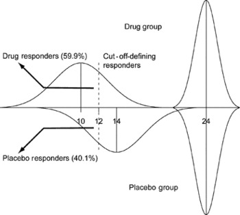
Consider now a study where our drug and placebo groups – which initially had the same mean score of 24 – differ after treatment by 4 points, with mean = 10 and 14, respectively, and SD = 8 in both. Figure 1 shows this situation. An appropriate ES for the means would be Hedges’g, which is 0.5. An ES of this magnitude is usually described as ‘medium’ and as such would imply non-trivial clinical interest.
Distributions of scores before and after treatment and the definition of responders (see text for further details).

If we prefer to describe outcome using responders and assume that our criterion was a score of 12 or less (Fig. 1), then 59.9% of the drug group and 40.1% of the placebo group will be responders. The difference of nearly 20 percentage points looks quite substantial, although the mean difference is unchanged. This difference in proportions also can be turned into an ES, and the two possibilities are d asin = 0.397 and d Cox = 0.485. So, the ES remains in the region of ‘medium’. Clearly, one way of not being misled by the ‘20%’ difference is to express it as an ES.
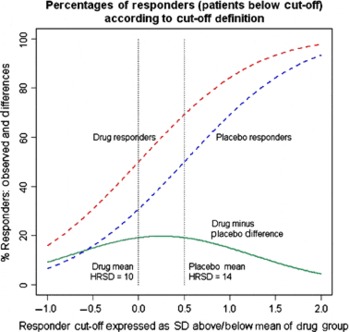
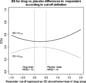
The relationship between ES and where the cut-off is drawn is not straightforward. In Fig. 2, we show how the percentage of responders in both groups changes as we shift the cut-off, where the cut-off is expressed as some number of SD units above or below the mean of the drug group. We can also see how the difference – in percentage points – changes. In Fig. 3, we have plotted our two ESs (d asin and d Cox): note how they are not in agreement and become less similar as the cut-off becomes more extreme. The choice of an ES measure is important. Remember also that irrespective of where the cut-off is placed, the value of Hedges’g remains at 0.5.
Percentages defined as responders under drug and placebo (and their difference) expressed in relationship to where the cut-off-defining responders is located.

ESs expressing differences between percentages of responders under drug and placebo expressed in relationship to where the cut-off-defining responders are located.

(The method of defining responders, based on changes of above a certain percentage, is potentially more complex, but for most purposes, the results look pretty much as above, and so we will not consider it further.)
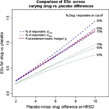
In Fig. 4, we examine how ESs alter according to the difference between drug and placebo at the end of treatment (from 2 to 10 HRSD points) as well as the percentage of patients on drug who are classified as responders (30, 50 and 70%). Much of this is unexceptional, although it is worth seeing the generally close relationship between Hedges’g and d Cox and the large differences between d asin.
ESs expressing differences between percentages of responders under drug and placebo expressed in relationship to drug vs. placebo mean difference and according to what percentage of the drug group are responders.

Returning to the Hedges’g ES, we note that a common way of describing how to interpret such an ES for means (here g = 0.50) is to point out that while 50% of patients in the drug group fall below the drug mean of 10, only 31% of patients in the placebo group fall below 10 (or 69 and 50%, respectively, fall below the mean of the placebo group). In other words, our sense of difference is being explained by an appeal to our sense of size as expressed in terms of percentage points, precisely what we might like to avoid! But, we get there precisely because one reason for using ESs is that our understanding of raw difference of X units has to be tempered by the SD of the groups and their overlap.
As shown in Fig. 4, let us assume that the medium clinical effect corresponds to 6 points. This is plausible because 3 points on the HRSD is often held to be the bare minimum difference of interest. Looking at the ESs above 6 on the x-axis, we can see they are close to 0.8, a value traditionally called ‘large’. What this might suggest to us is that we need to recalibrate these adjectives: a medium ES for the HRSD might better be one of around 0.8 and not 0.5. This really should not surprise us because the original classification drew on particular areas of psychological research, and there was no intent for them to be universal. And if we want to use percentage responding, then we really should turn it into an ES using d Cox.
The Kirsch and Moncrieff article is a timely reminder. Their concern about the use of responders vs. non-responders distinction has not been answered here, but understanding percentages and understanding mean differences seem to work off each other, and ES remains as an attractive tool.