Statistical mechanics and molecular dynamics in evaluating thermodynamic properties of biomolecular recognition

Jeff Wereszczynski; J. Andrew McCammon

doi:10.1017/S0033583511000096

Statistical mechanics and molecular dynamics in evaluating thermodynamic properties of biomolecular recognition

Published online by Cambridge University Press: 15 November 2011

Jeff Wereszczynski and

J. Andrew McCammon

Show author details

Jeff Wereszczynski*: Affiliation:
Department of Chemistry and Biochemistry, University of California, San Diego, CA, USA
J. Andrew McCammon: Affiliation:
Department of Chemistry and Biochemistry, Department of Pharmacology, Howard Hughes Medical Institute, Chevy Chase, MD, USA
*: *Author for correspondence: J. Wereszczynski, Department of Chemistry and Biochemistry, University of California, San Diego, CA, USA. Tel.: 858.822.0169; Fax: 858.534.4974; Email: jmweresz@mccammon.ucsd.edu

Article contents

Abstract
Introduction
Theoretical basis of entropy and free energy calculations
Methods for calculating free energy and entropy differences
Interesting results
Conclusion
References

Rights & Permissions

Abstract

Molecular recognition plays a central role in biochemical processes. Although well studied, understanding the mechanisms of recognition is inherently difficult due to the range of potential interactions, the molecular rearrangement associated with binding, and the time and length scales involved. Computational methods have the potential for not only complementing experiments that have been performed, but also in guiding future ones through their predictive abilities. In this review, we discuss how molecular dynamics (MD) simulations may be used in advancing our understanding of the thermodynamics that drive biomolecular recognition. We begin with a brief review of the statistical mechanics that form a basis for these methods. This is followed by a description of some of the most commonly used methods: thermodynamic pathways employing alchemical transformations and potential of mean force calculations, along with end-point calculations for free energy differences, and harmonic and quasi-harmonic analysis for entropic calculations. Finally, a few of the fundamental findings that have resulted from these methods are discussed, such as the role of configurational entropy and solvent in intermolecular interactions, along with selected results of the model system T4 lysozyme to illustrate potential and current limitations of these methods.

Information

Type: Review Article
Information: Quarterly Reviews of Biophysics , Volume 45 , Issue 1 , February 2012, pp. 1 - 25
DOI: https://doi.org/10.1017/S0033583511000096 [Opens in a new window]
Copyright: Copyright © Cambridge University Press 2011

1. Introduction

A key component of the physical basis for many cellular functions, such as molecular trafficking, signal transduction, and genetic expression, is the non-covalent interaction of biomolecules with themselves and one another, a process referred to as biomolecular recognition (Gellman, Reference Gellman1997; McCammon, Reference McCammon1998). Understanding biomolecular recognition is therefore of prime importance not only for advancing our knowledge of chemistry and biology, but also in the development of therapeutics for the treatment of disease. Although based on the laws of physics, this is inherently complicated due to the range of potential interactions (hydrophobic, electrostatic, etc.), the complex interaction networks between groups of atoms in both the biomolecules and their surrounding solvent, and the multiple timescales upon which events occur. It is therefore not surprising that a wealth of experimental and computational tools have been developed to probe these processes, each of which possesses its own strengths and weaknesses.

There are several experimental techniques that have proved invaluable in the study of biomolecular recognition. For example, X-ray crystallography and NMR methods provide atomic-resolution, three-dimensional structures of biomolecules. These methods describe not only the intra- and intermolecular orientation of molecules in a complex but also order parameters (the B-factor in crystallography and S ² in NMR) may give details about the degree of local motions in the observed state (Petsko & Ringe, Reference Petsko and Ringe1984; Stone, Reference Stone2001; Zidek et al. Reference Zidek, Novotny and Stone1999). Isothermal titration calorimetry (ITC) can be used to accurately measure not only the free energy change associated with biomolecular recognition, but also to decompose it into enthalpic and entropic contributions (Ladbury & Chowdhry, Reference Ladbury and Chowdhry1996; Olsson et al. Reference Olsson, Williams, Pitt and Ladbury2008). Still, it is difficult to get a complete picture of intermolecular interactions from experiments alone, hence computational work may be helpful in not only interpreting observed results but also in guiding future experiments. Molecular dynamics (MD) simulations, in which each atom of a system is allowed to evolve over time under the forces acting on it by the rest of the system, have become an important tool in the study of biomolecules, as they offer atomic-resolution models for the system of interest (Adcock & McCammon, Reference Adcock and McCammon2006; Gilson & Zhou, Reference Gilson and Zhou2007; Guvench & MacKerell, Reference Guvench and MacKerell2009; Levy & Gallicchio, Reference Levy and Gallicchio1998). Current methods and computing power allow for the simulation of systems under a million atoms (large enough for a majority of proteins of interest) for hundreds of nanoseconds, boundaries that are constantly being pushed back by continued developments in computer architecture and design (Shaw et al. Reference Shaw, Deneroff, Dror, Kuskin, Larson, Salmon, Young, Batson, Bowers, Chao, Eastwood, Gagliardo, Grossman, Ho, Ierardi, Kolossváry, Klepeis, Layman, McLeavey, Moraes, Mueller, Priest, Shan, Spengler, Theobald, Towles and Wang2008; Stone et al. Reference Stone, Phillips, Freddolino, Hardy, Trabuco and Schulten2007).

In this review, we provide an introduction to the use of MD simulations in the calculations of thermodynamic properties important to biomolecular recognition. To lay the theoretical framework for methods used in the field, we begin with a brief overview of the statistical mechanics that underlie the methods, specifically discussing the origins of the microcanonical and canonical ensembles, and their relation to free energy and the equilibrium binding constant. We recognize that some may find this section overly technical, therefore we have structured the remainder of this review such that this section may be skimmed on an initial reading without a significant loss. Then we discuss a few of the major methods used for the computation of free energy differences, such as alchemical transformation, potential of mean force, and end point calculations, followed by a description of methods for the determination of conformational entropies. We conclude with a discussion of a few interesting results that highlight the utility of these tools, first in the general areas of the role conformational entropy and solvent play in biomolecular recognition, then to the specific case of T4 lysozyme which has become a model system for the study of protein–ligand interactions. We do not discuss the important details of the MD ‘force-field’, although the interested reader may find these in one of several reviews (Best et al. Reference Best, Buchete and Hummer2008; Mackerell, Reference Mackerell2004).

2. Theoretical basis of entropy and free energy calculations

2.1 A brief review of statistical mechanics

If one is interested in the thermodynamic properties of a system containing N particles, then in theory these may be determined by solving the 3N Newtonian equations of motion for infinite sampling time. In practice, this is both impossible and unnecessary. It is impossible in that, until the development of MD simulations, only the deterministic equations for systems composed of a handful of particles could be solved, and even with modern computing resources simulations are limited both in size and length. However, instead of considering the deterministic motions of its particles, a wealth of information may be obtained about a particular system by concentrating on its probabilistic configurations. This is the field of statistical mechanics, which treats systems at equilibrium by probability functions, and with some elementary assumptions, connects the microstates of a system to macroscopic thermodynamic quantities (such as temperature, chemical potential and free energy). The increasing popularity of MD, which solves the Newtonian equations of motion for each atom in a system, makes recognizing the connection between statistical mechanics with thermodynamics particularly relevant for understanding how we deal with the thermodynamics of molecular recognition. Therefore, we start this section with a brief review of the microcanonical and canonical ensembles from statistical mechanics. For brevity, this review is not meant to be complete, and the reader is referred to one of many outstanding textbooks or reviews on the subject (Chandler, Reference Chandler1987; Kirkwood, Reference Kirkwood1935; Toda et al. Reference Toda, Kubo and Saitô1992; Zhou & Gilson, Reference Zhou and Gilson2009).

2.1.1 The microcanonical ensemble

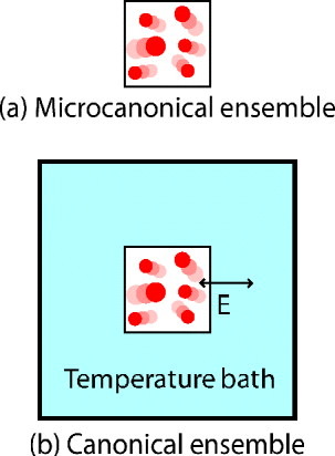
We begin to examine the microscopic realm by considering a system of classical particles that is isolated from the outside world such that the macroscopic properties N (number of particles), V (the volume), and E (the total energy of the system) remain constant (as is illustrated in Fig. 1). Such a system is referred to as the microcanonical ensemble or the NVE ensemble (for constant Number, Volume, and Energy). This system can be in one of Ω accessible microstates. If one assumes that transitions to and from each microstate are permissible (the ergodic hypothesis), then the principle of equal probability states that each is equally likely with probability:

(1)

$p_{i} \equals 1\sol \rmOmega .$

Boltzmann derived that the entropy of a system, S, is related to a weighted sum of the logarithms of each accessible state, that is

(2)

$S \equals \minus k\sum\limits_{{\rm states}} {p_{i} \log p_{i} } \comma$

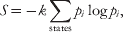
where k is the Boltzmann constant. Substituting Eq. (1) into Eq. (2) we arrive at the famous definition for entropy:

(3)

$S \equals k\log \rmOmega .$

This fundamental equation states that the entropy of a system (a macroscopic quantity) is directly related to the number of accessible microscopic states.

Fig. 1.

The microcanonical ensemble (a) consists of a constant number of particles (N) in a box of constant volume (V) with constant energy (E) that are isolated from the outside world. The canonical ensemble (b) is an extension of this ensemble, in which N and V are still constants, but the system is allowed to exchange energy with the outside world while the temperature (T) is a constant.

While there are several interesting results that may be derived from this model, the one most relevant to our discussion concerns the interactions of two microcanonical ensembles. If two microcanonical systems are interacting such that they are allowed to exchange energy but not particles or other macroscopic quantities with one another, then the total energy of the system may be defined as E _I+E _II=E _Total. The total number of states for both systems is represented by the product of the number of states for the smaller systems (each of which is a function of their energy), that is

(4)

$\rmOmega _{{\rm Total}} \equals \rmOmega _{\rm I} \lpar E_{\rm I} \rpar \rmOmega _{{\rm II}} \lpar E_{{\rm II}} \rpar \equals \rmOmega _{\rm I} \lpar E_{\rm I} \rpar \rmOmega _{{\rm II}} \lpar E_{{\rm Total}} \minus E_{\rm I} \rpar .$

The most probable energy distribution between the two systems corresponds to the value of E _I that maximizes the value of Ω_Total, which also corresponds to the maximum entropy of the combined system (in accord with the second law of thermodynamics). As it is at a maximum, we may set the first derivative of the combined system entropy to zero, yielding:

(5)

${{{\rm d}\ln \rmOmega _{{\rm Total}} \lpar E_{\rm I} \rpar } \over {{\rm d}E_{\rm I} }} \equals {{{\rm d}\ln \rmOmega _{\rm I} \lpar E_{\rm I} \rpar } \over {{\rm d}E_{\rm I} }} \minus {{{\rm d}\ln \rmOmega _{{\rm II}} \lpar E_{{\rm Total}} \minus E_{\rm I} \rpar } \over {{\rm d}\lpar E_{{\rm Total}} \minus E_{\rm I} \rpar }} \equals 0\comma$

which, with some reorganizations, results in

(6)

${{{\rm d}\ln \rmOmega _{\rm I} \lpar E_{\rm I} \rpar } \over {{\rm d}E_{\rm I} }} \minus {{{\rm d}\ln \rmOmega _{{\rm II}} \lpar E_{{\rm Total}} \minus E_{\rm I} \rpar } \over {{\rm d}\lpar E_{{\rm Total}} \minus E_{\rm I} \rpar }} \equals 0.$

Since Ω_I and Ω_II may be unique from one another, their first derivatives are equal if and only if they are constant, which we have defined as the value of β. It can be shown that β has the property that it is inversely related to the absolute temperature T, that is β=1/kT. Systems I and II are said to be in thermal equilibrium when only small energy transfers between the two systems are observed as system I fluctuates around an equilibrium energy value of E _I* and system II around energy E _Total−E _I*.

2.1.2 The canonical ensemble

In the microcanonical ensemble, a system completely isolated from the outside world with a constant number of particles N, constant volume V and constant energy E is considered. However, for our purposes, a more pertinent system is one that still has a constant N and V, but that is in thermal equilibrium with its environment and thus has a non-constant E but a constant temperature T (see Fig. 1b). This is the canonical, or NVT (constant Number, Volume, and Temperature), ensemble. This may be thought of as a special case of the two interacting microcanonical systems in which one system (system II) is much larger than its counterpart (system I), and is often referred to as a heat bath or heat reservoir. The total energy and number of states for each system and the combined systems are defined as E _I and Ω_I, for i=I, II, Total. If we take Eq. (4), and set the total number of states to a constant, Ω_Total=1/C, rearrangement of terms yields:

(7)

${1 \over {\rmOmega _{\rm I} \lpar E_{\rm I} \rpar }} \equals C\rmOmega _{\rm II} \lpar E_{{\rm Total}} \minus E_{\rm I} \rpar .$

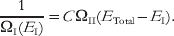
Using the principle of equal probability Eq. (1), we note that the probability of observing system I in a state with energy E _I is entirely dependent on the number of states in the heat bath (system II) at energy E _Total−E _I. That is

(8)

$\rho _{\rm I} \lpar E_{\rm I} \rpar \equals C\rmOmega _{{\rm II}} \lpar E_{{\rm Total}} \minus E_{\rm I} \rpar .$

The assumption that system II is much larger than system I implies that E _Total≈(E _Total−E _I), thus we may take the logarithm of each side and perform a Taylor expansion about the point E _Total to the term containing Ω_II to obtain:

(9)

$\ln \left( {\rho _{\rm I} \lpar E_{\rm I} \rpar } \right) \equals C\prime {{{\rm d}\ln \rmOmega _{{\rm II}} \lpar E\rpar } \over {{\rm d}E}}E_{\rm I} .$

Borrowing from Eq. (6) and exponentiating each side of Eq. (9) we find that, when normalized over all possible states j, the probability for system I to exist in a microstate n with energy E_n is

(10)

$\rho _{\rm I} \lpar E_{n} \rpar \equals {{\exp \hskip-1pt \lpar \minus \beta E_{n} \rpar } \over {\sum\limits_{j} {\exp \hskip-1pt \lpar \minus \beta E_{j} \rpar } }} \equals {{\exp \hskip-1pt \lpar \minus \beta E_{n} \rpar } \over Z}.$

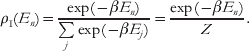
Equation (10) is one of the fundamental equations in statistical mechanics. It states that, unlike in the microcanonical ensemble where the system is evenly distributed among microstates with a specific energy, in the canonical ensemble interactions with a heat bath cause the energy of the system to fluctuate, with representative points in phase space distributed by the factor exp(−βE), the Boltzmann factor. In addition, although the system and the heat bath are coupled, the assumption that the heat bath (system II) is much larger than system I means that the thermodynamic properties of system I may be solved for with knowledge of only the term β (the inverse temperature, β=1/kT, where k is the Boltzmann constant) from system II. To compute thermodynamic averages of a physical quantity A, a weighted average of A is computed based on the Boltzmann factor.

The denominator of Eq. (10), which has been introduced to normalize the probability of states and is denoted as Z, is referred to as the partition function of the ensemble. The partition function is a particularly important concept. All thermodynamic quantities may be expressed in terms of it, which therefore implies that knowledge of the partition function is sufficient for understanding the macroscopic properties of a system. For example, by substituting Eq. (10) into Eq. (2), we recover the definition of entropy in the canonical ensemble, which depends solely on the average enthalpic energy U and Z:

(11)

$S \equals k\beta U \plus k\ln Z.$

From thermodynamics, we know that the maximum amount of work a system can do, the Helmholtz-free energy, is defined as a difference of enthalpic (the internal energy, U) and entropic (TS) terms F=U−TS. By substituting Eq. (11) into this relation, we obtain

(12)

$F \equals U \minus TS \equals \minus kT\ln Z.$

Therefore, we see that computing the partition function is the fundamental challenge in computing thermodynamic properties for equilibrium processes, including molecular recognition. For classical systems, it is convenient to describe the accessible energies as a function of the system's momentum and position vectors (6N coordinates), and if we assume these are continuous variables (as opposed to quantum ones), then the partition function may be rewritten as

(13)

$Z \equals \sum\limits_{j} {\exp \hskip -2pt \lpar \minus \beta E_{j} \rpar \propto \int\hskip -6pt \int {\exp \left[ { \minus \beta H\lpar x\comma p\rpar } \right]{\rm d}x{\rm d}p} } \comma$

where H(x, p), the Hamiltonian, is the total energy composed of a sum of the kinetic and potential energies (determined by the momentum and position values). The canonical ensemble assumes a constant number of particles, volume and temperature; however, it is often desirable to consider a system in which the volume is allowed to fluctuate to maintain a constant pressure. This is referred to as the isothermal–isobaric, or NPT (constant Number, Pressure, and Temperature), ensemble. Derivation of this ensemble is similar to the canonical ensemble, with the major difference being the weight of a microstate becomes exp[−β(E+PV)], with a corresponding modification to the partition function. The appropriate free energy becomes the Gibbs free energy (G), which is similar to the Helmholtz free energy except for a modification to the enthalpic term to account for the system volume. That is

(14)

$G \equals U \plus PV \minus TS \equals \minus kT\ln Z.$

As a more general case, the system of interest may be allowed to exchange particles with its environment in the Grand Canonical Ensemble, where the chemical potential is considered a constant instead of the number of particles in the system. In general, the canonical ensemble provides a sufficient description for our purposes, making the grand canonical ensemble beyond the scope of this review. For details on either of these cases, the interested reader is referred to a statistical physics textbook, such as Toda et al. (Reference Toda, Kubo and Saitô1992) .

2.1.3 Equilibrium binding constant

Let us consider the case of a ligand L and a receptor R in chemical equilibrium, such that the [L], [R] and [LR] are the concentrations of the free ligand, free receptor, and bound ligand–receptor complex, which are invariant over time. Then, the equilibrium constant K _b for the reaction [L]+[R]⇌[LR] is defined as

(15)

$K_{\rm b} \equals {{\lsqb LR\rsqb } \over {\lsqb L\rsqb \lsqb R\rsqb }}.$

If we take the view of a single receptor molecule, the probabilities for observing this receptor bound to and free from a ligand, P _bound and P _free, respectively, are proportional to the solution concentrations [LR] and [R], such that Eq. (15) becomes

(16)

$K_{\rm b} \equals {1 \over {\lsqb L\rsqb }}{{P_{{\rm bound}} } \over {P_{{\rm free}} }}.$

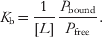
To determine the ratio of any ligand bound to the unbound receptor, P _bound/P _free, let us focus on the probability of the receptor being bound to (state 1) or free from a particular ligand (state 0), P ₁/P ₀. The probability of each of these states may be expressed in terms of the system's partition function over the space in which ligand L is bound or in bulk. That is

(17)

$P_{{\rm bound}} \propto \int_{{\rm bound}} {\exp \left[ { \minus \beta H\lpar x\comma p\rpar } \right]} {\rm d}x\comma$

where we have omitted the integration over momentum space from Eq. (13) for simplicity. If we assume that the bulk solution is homogeneous, then a point x*, which is sufficiently far from the receptor to prevent ligand–protein interaction, may be arbitrarily chosen such that

(18)

${{P_{\setnum{1}} } \over {P_{\setnum{0}} }} \equals {{\int_{{\rm bound}} {\exp \hskip -2pt \lsqb \minus \beta H\rsqb {\rm d}x} } \over {V_{{\rm bulk}} \int_{{\rm bulk}} {\delta \lpar x_{l} \minus x^{\ast } \rpar \exp \hskip -2pt \lsqb \minus \beta H\rsqb {\rm d}x} }}\comma$

where V _bulk is the volume of the bulk solution and x_l is the ligand's position. Since the ligands are identical, the probability for any one of the N ligands in solution to be bound to the receptor is simply N⋅P ₁/P ₀, which is equivalent to the ratio P _bound/P _free. Therefore, Eq. (16) becomes

(19)

$K_{\rm b} \equals {1 \over {\lsqb L\rsqb }}{{N\int_{{\rm bound}} {\exp \hskip -2pt\lsqb \minus \beta H\rsqb {\rm d}x} } \over {V_{{\rm bulk}} \int_{{\rm bulk}} {\delta \lpar x_{l} \minus x^{\ast } \rpar \exp \hskip -2pt \lsqb \minus \beta H\rsqb {\rm d}x} }} \equals {{Z_{{\rm bound}} } \over {Z_{{\rm free}} }}\comma$

where Z _bound is the partition function over states with the ligand in the binding pocket, and Z _free for states when the ligand is a distance x* away. If one takes the natural log of Eq. (19) and multiplies by −kT, then by using Eq. (12), we recover the familiar expression:

(20)

$\minus kT\ln \hskip -2pt\lpar K{}_{b}\rpar \equals \minus kT\lpar \ln Z_{{\rm bound}} \rpar \plus kT\ln Z_{{\rm free}} \equals F_{{\rm bound}} \minus F_{{\rm free}} .$

That is, the natural log of the equilibrium binding constant is the difference in free energy between a ligand in a free state (typically referred to as infinitely far away) and one in a bound state. As a matter of convenience, F _free is typically defined as 0. This derivation relies solely on the canonical ensemble (Deng & Roux, Reference Deng and Roux2006). An alternative derivation based on the chemical potentials of the species L, R and LR may be derived from the grand canonical ensemble with similar results (Gilson et al. Reference Gilson, Given, Bush and McCammon1997a).

3. Methods for calculating free energy and entropy differences

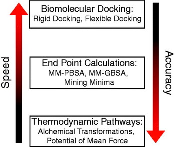
From the previous section, we see that the calculation of free energy and entropy differences is possible by considering each accessible microstate of the system, and its corresponding energy, to determine the partition function for use in Eqns. (11) and (12). To do this requires significant computation, which is impractical for even small systems. However, we are generally concerned with a free energy difference (as in Eq. (20)), and not the absolute free energy of a system. Several methods have been developed to sample the regions of phase space most important to the recognition process, thereby providing approximations to free energy and entropy changes of a system, which have a trade-off between speed and accuracy (see Fig. 2). For example, docking methods may estimate the free energy gained when a ligand binds to the binding site of a protein without any previous knowledge of the bound state in a matter of minutes, but the error in the free energies tends to be quite high. In contrast, free energies estimated via alchemical transformations tend to correlate much better to experimental values, yet they not only require knowledge of the bound state but may also require hundreds or thousands of computer hours. Here, we discuss two major techniques used in the field for calculating free energy differences: thermodynamic pathways and end point calculations, followed by a discussion of methods that exist for the calculation of the conformational entropy component of a system. For further details on docking, the reader is referred to one of the many reviews on the subject (Brooijmans & Kuntz, Reference Brooijmans and Kuntz2003; Durrant & McCammon, Reference Durrant and McCammon2010; Fuentes et al. Reference Fuentes, Dastidar, Madhumalar and Verma2011; Halperin et al. Reference Halperin, Ma, Wolfson and Nussinov2002; Kitchen et al. Reference Kitchen, Decornez, Furr and Bajorath2004; Klebe, Reference Klebe2006).

Fig. 2.

The major types of free energy calculations can be divided into three categories: biomolecular docking, end point and thermodynamic pathway calculations. In general, there is a trade-off between the speed and accuracy of these methods.

3.1 Thermodynamic pathways

In Section 2.1, we derived Eq. (12), which states that the absolute free energy of a system is related to the partition function Z. To compute the free energy change of a biomolecular process, such as binding of a ligand to a protein, one could compute the partition functions of the system before and after the molecular association (Z ₀ and Z ₁), and subtract the logarithms of the two. However, this requires extensive sampling of phase space for both states, a task that is difficult for small systems and nearly impossible for protein-sized ones. If we take advantage of the fact that (in general) we are interested in the change in free energy of a system, ΔF, we may instead focus on this by computing:

(21)

$\rmDelta F_{\setnum{0} \minus \gt \setnum{1}} \equals \minus kT\ln {{Z_{\setnum{1}} } \over {Z_{\setnum{0}} }}.$

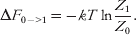
If we assume a classical system, as is described in Eq. (13), then the microstates that are identical between the two macrostates cancel each other out, and our problem simplifies to calculating the portions of phase space which differ from one another in states 0 and 1. Several methods have been developed to solve Eq. (21), which rely on enhancing sampling along one or a few dimensions known as the ‘reaction coordinate(s)’ (that we denote as ξ), which may be largely divided into two categories. In the first, ξ is constrained such that it has only a single value over the simulation, and the free energy between states is calculated by either a direct calculation of Eq. (21) or by integration of the derivative of dF/dξ. In the second class of methods, ξ is biased with a restraint that enhances sampling of phase space for regions which have a low probability of being visited in standard simulations. By utilizing knowledge of the biased probability functions P*(ξ) along with the form of the bias, one may recover free energy profiles along ξ, and thus the free energy difference between states 0 and 1.

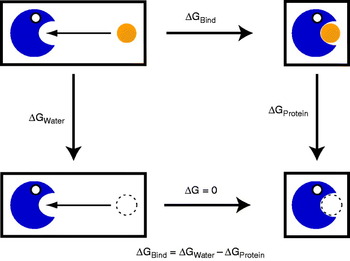
Keeping with the example of a ligand binding to the binding site of a protein, Fig. 3 shows two potential pathways for calculating the free energy of binding. In the direct method, ΔG _bind may be obtained directly by computing the free energy along a physical pathway that takes the ligand from a distance far away from the binding pocket into it. For systems in which the ligand binds to a solvent exposed site on the protein, this may be an appropriate method as it is direct and (relatively) straightforward. However, for many systems, such as T4 lysozyme (see Section 4.3), the binding site is partially or fully hidden from solvent, requiring significant conformational rearrangement of the protein upon binding that may be difficult to sample with physical pathways. As an alternative, one can draw a thermodynamic cycle (as in Fig. 3) that connects the free and bound states through unphysical pathways that relies on transferring the ligand from its original system into a vacuum, which is termed ‘annihilation’ or ‘decoupling’. This requires two sets of calculation. In the first, ΔG _water is computed as the free energy of decoupling the unbound ligand from its interactions with solvent, while in the second, ΔG _protein is the free energy of decoupling from the bound protein state. The free energy of moving a decoupled ligand into the binding site of a protein is zero (since it is not interacting with the system, the bottom path in Fig. 3) so the binding free energy may be computed as ΔG _bind=ΔG _water−ΔG _protein (Chipot & Pohorille, Reference Chipot and Pohorille2007).

3.1.1 Constrained free energy calculations

To solve Eq. (21), let us define the Hamiltonian of system 1 as a sum of the Hamiltonian of system 0 plus a perturbation term ΔH=ΔU (where ΔU is a change in potential energy). If we substitute this term into the partition function for state 1, and we utilize Eq. (10) for the probability of observing state 0 to have a specified Hamiltonian, it can be shown that the free energy of going from state 0 to 1 is (Straatsma & McCammon, Reference Straatsma and McCammon1992; Zwanzig, Reference Zwanzig1954):

(22)

$\rmDelta F_{\setnum{0} \minus \gt \setnum{1}} \equals \minus kT\ln \left\langle {\exp \lpar \minus \beta \rmDelta U\rpar } \right\rangle_0.$

That is, in free energy perturbation (FEP), the free energy difference between states 0 and 1 may be calculated by the natural log of the average Boltzmann factor of the potential energy difference between states 1 and 0 over equilibrium configurations from state 0. The value ΔU may be thought of as the work required to instantaneously transform the system from state 0 to 1. In principle, this is a thermodynamically exact relation, but in practice if the energy ΔU is larger than a few kcal/mol, the exponential term creates computational havoc and produces unreliable results. If there is a large perturbation to the system (such as the decoupling of a ligand from solvent or a protein's binding site), then it is advantageous to divide the free energy into smaller segments, or ‘windows’, which follow an order parameter λ such that the Hamiltonian for a system with a λ value is defined as

(23)

$H\lpar \lambda \rpar \equals \lambda H_{\setnum{1}} \plus \lpar 1 \minus \lambda \rpar H_{\setnum{0}} .$

Such a transformation between two physical end states through an unphysical pathway is termed an alchemical free energy calculation. In practice, one performs a series of simulations with λ values varying between 0 and 1, and through utilization of Eq. (22) the free energy between successive windows is calculated. The total free energy to go from states 0 to 1 is therefore the sum of the free energies between each of the simulated λ-points.

Fig. 3.

The thermodynamic cycle used in free energy calculations. Potential of mean force calculations attempt to compute ΔG _bind directly by computing the free energy along a path to bring a ligand into a protein's binding pocket. Alchemical transformations take an alternative route by calculating ΔG _water and ΔG _protein through decoupling of the ligand from a solvated and protein-bound environment, respectively. Because free energy is a state function, and the bottom leg of the free energy cycle equals zero (since in that part nothing is moved into the protein's binding pocket) ΔG _bind may be calculated as the difference of ΔG _water and ΔG _protein.

Increasing the number of windows in an alchemical transformation may decrease the variance in the calculated free energies, yet the exponential averaging in FEP may still produce numerical errors. Therefore, alternative methods have been developed to improve the convergence of calculated free energies. In thermodynamic integration (TI) the derivative of H with respect to λ, followed by integration of λ from 0 to 1, is used to compute ΔF (Straatsma & McCammon, Reference Straatsma and McCammon1991, Reference Straatsma and McCammon1992):

(24)

$\rmDelta F_{\setnum{0} \minus \gt \setnum{1}} \equals \int_{\setnum{0}}^{\setnum{1}} {\displaystyle\left\langle {{{{\rm d}H\lpar \lambda \rpar } \over {{\rm d}\lambda }}} \right\rangle }_\lambda \hskip 2pt {\rm d}\lambda .$

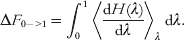
For the case of an alchemical transformation, the dH(λ)/dλ term reduces to the derivative of the electrostatic potential plus the derivative of the van der Waals potential terms with respect to λ for the part of the system which varies between the two endpoints, both of which have analytic solutions. One caveat of TI is that, since λ has discrete values, it relies on proper integration techniques (Jorge et al. Reference Jorge, Garrido, Queimada, Economou and Macedo2010). A newer alternative for improving the convergence of alchemical transformations was recently introduced by Shirts et al., in which the free energy between two λ points may be estimated by using the work functions from both windows in the maximum likelihood estimator developed by Bennett (Shirts et al. Reference Shirts, Bair, Hooker and Pande2003). The Bennett acceptance ratio (BAR) provides the optimal asymptotically unbiased estimate of the free energy difference (Shirts & Pande, Reference Shirts and Pande2005). The multistate Bennett acceptance ratio (MBAR) was later developed as a generalization to BAR that incorporates work functions between all windows into the estimator, resulting in further reduced variances of the calculated free energies (Shirts & Chodera, Reference Shirts and Chodera2008).

Regardless of the free energy estimator used (FEP, TI, BAR, or MBAR), there are several practical challenges in alchemical free energy transformations (Shirts et al. Reference Shirts, Mobley and Chodera2007). The first is that all of these methods rely on extensive sampling of the equilibrium state of the system in each λ point, which may require several nanoseconds for the decoupling of a ligand bound to a protein. Even with several nanoseconds of simulations, simulations may become trapped in metastable states, resulting in free energy estimates that may not accurately represent the complete ensemble of bound and unbound conformations. This may partially be avoided through multiple free energy calculations (Lawrenz et al. Reference Lawrenz, Baron and McCammon2009) or through the use of enhanced sampling techniques to improve phase space sampling (Fajer et al. Reference Fajer, Hamelberg and McCammon2008; Hamelberg et al. Reference Hamelberg, Mongan and McCammon2004; Jiang & Roux, Reference Jiang and Roux2010; Wereszczynski & McCammon, Reference Wereszczynski and McCammon2010; Woods et al. Reference Woods, Essex and King2003), both of which are active fields of research. In addition, special problems exist for the states in which the protein–ligand interactions are nearly entirely eliminated, such as excessive sampling of the simulation box by the ligand and numerical instabilities, both of which may be addressed by the introduction of restraining (Hamelberg & McCammon, Reference Hamelberg and McCammon2004; Wang et al. Reference Wang, Deng and Roux2006) and soft-core potentials (Beutler et al. Reference Beutler, Mark, Vanschaik, Gerber and van Gunsteren1994; Zacharias et al. Reference Zacharias, Straatsma and McCammon1994).

3.1.2 Free energy pathways via biased simulations

As an alternative, the free energy between two states may be derived through the probability of observation of those states. If we have a state, 0, then the probability of observing this state (P ₀) is proportional to its partition function, Z ₀. Thus, when determining the free energy difference between states 0 and 1, Eq. (21) may be rewritten as

(25)

$\rmDelta F \equals \minus kT\ln {{P_{\setnum{1}} } \over {P_{\setnum{0}} }}.$

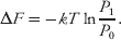
Determining the probability of observing one state over another is therefore equal to determining the free energy difference. One could perform a simulation and directly determine the free energy difference by counting the number of configuration in states 0 and 1 and use these values as unnormalized probabilities in Eq. (25) (Thomas & Elcock, Reference Thomas and Elcock2006). However, if these states are separated by energy barriers of even a few kcal/mol, or significant diffusion is required to process from one state to another, then the simulation length required to directly compute ΔF may easily be several orders of magnitude more than what is available by today's computers. To alleviate this practical problem, several methods have been developed which enhance the sampling of phase space through biased simulations and, with proper reweighting, allow for the calculation of an unbiased ΔF.

Perhaps the most widely used of these methods is umbrella sampling (Torrie & Valleau, Reference Torrie and Valleau1977). In umbrella sampling, sampling of phase space is enhanced by biasing the simulation with an additional potential, the umbrella potential, along one (or a few) reaction coordinate(s). The choice of the reaction coordinate is critical, as it is assumed that motions along this dimension dominate the free energy of the observed changes in the system. In some cases, the choice of a reaction coordinate is straightforward, for example, when pulling a ligand out of a protein's binding site the center of mass separation distance may suffice, while in other cases more complex reaction coordinates may be required. Still, if we assume that the motions along the reaction coordinate(s) are sufficient for describing the system, then by utilizing several simulations with umbrella potentials that span the interesting regions of the reaction coordinate, sampling of phase space may be dramatically improved relative to unbiased simulations. The weighted histogram analysis method (WHAM) may then be used to combine the probability distributions from the multiple biased simulations into a single unbiased probability profile, which, when used with Eq. (25), produces a free energy profile along the reaction coordinate(s) (Kumar et al. Reference Kumar, Bouzida, Swendsen, Kollman and Rosenberg1992; Roux, Reference Roux1995).

Other biased simulations techniques, such as adaptive biasing force (Darve et al. Reference Darve, Rodriguez-Gomez and Pohorille2008) and metadynamics (Laio & Parrinello, Reference Laio and Parrinello2002), are also routinely used for calculating free energy profiles related to conformational transitions in biomolecules. In both of these methods, an external bias is adaptively added to the simulation based on the conformational space sampled at a particular time, making unnecessary the use of multiple simulation windows for sampling a wide region of phase space (although they may be employed if desired). While these methods do have practical advantages and can increase the convergence rate for some systems, slow conformational changes may benefit more from traditional umbrella sampling techniques that actively force sampling of phase space instead of relying on diffusion of the biased systems along the reaction coordinate(s).

3.1.3 Emerging free energy methods

While there are several novel methods for the calculation of free energy differences relating to biomolecular recognition processes, for brevity we highlight two of these methods to provide the reader with a flavor of these emerging techniques. One interesting method combines the ideas of alchemical transformations, in which the Hamiltonian is defined by the parameter λ (Eq. (23)) with biased simulation techniques. In λ-dynamics, the λ parameter is a dynamical variable that fluctuates throughout a simulation based on Newtonian mechanics with a fictitious mass and a biasing potential (Knight & Brooks, Reference Knight and Brooks2009; Kong & Brooks, Reference Kong and Brooks1996). In this way, a ligand can ‘appear’ and ‘disappear’ to a protein several times throughout a single simulation, which may have the advantages of enhancing sampling by avoiding conformational traps and negating the necessity of multiple simulation windows. Additionally, a series of ligands may be simulated in a single run (each with their own λ values) which may further improve computational efficiency. Analogously, simulations may be performed in which an unphysical fourth spatial dimension is introduced, along which the free energy of removing the ligand from a protein's binding site may be calculated with methods such as umbrella sampling (Beutler & van Gunsteren, Reference Beutler and van Gunsteren1994; Rodinger et al. Reference Rodinger, Howell and Pomes2005).

As mentioned above, the relative free energy difference between two states may be reliably calculated if the simulation sufficiently samples both endpoints, negating the need for intermediate states. In the one-step perturbation technique, a single unphysical state (the ‘reference’ state) is simulated which has a partition function that is the sum of the two end states (Oostenbrink & van Gunsteren, Reference Oostenbrink and van Gunsteren2003, Reference Oostenbrink and van Gunsteren2005). In theory, this should enhance sampling of the important regions of phase space for both endpoints; however, in practice, this may be complicated if the Hamiltonians of the two states differ significantly. This method has evolved into envelope-distribution sampling with the introduction of an iterative method for the calculation of an ideal reference state, which has a straightforward extension to the case of calculating relative free energies between multiple end states (instead of just two) (Christ & van Gunsteren, Reference Christ and van Gunsteren2007, Reference Christ and van Gunsteren2008). While these simulations may still require significant simulation time for convergence, they show promise in the calculation of multiple free energies from a single run. For example, they may be useful in calculating the free energy change resulting in the modification of a ligand's functional group to multiple possible end states, a key problem in the lead optimization stage of a drug-design project.

3.2 End point calculations

Calculations of free energy differences based on thermodynamic pathways tend to require extensive sampling of conformations not only at the end points of interest but also in between, thus requiring sizeable computational cost. A computationally less expensive approach is to simulate only the two end states of interest (such as a protein free from and bound to a ligand) to estimate their absolute free energies, and to subtract them from one another (Gilson et al. Reference Gilson, Given, Bush and McCammon1997a, Reference Gilson, Given and Headb; Swanson et al. Reference Swanson, Henchman and McCammon2004). Keeping with the example of a ligand binding to a receptor, the free energy gained through binding is

(26)

$\rmDelta G_{{\rm bind}} \equals G_{{\rm complex}} \minus \lpar G_{{\rm receptor}} \plus G_{{\rm ligand}} \rpar$

Each of these free energies is then decomposed into four terms:

(27)

$G \equals \left\langle {E_{{\rm MM}} } \right\rangle \minus T\left\langle {S_{{\rm MM}} } \right\rangle \plus \left\langle {G_{{\rm Solv}} } \right\rangle \plus \left\langle {G_{{\rm np}} } \right\rangle \comma$

where 〈E _MM〉 represents the mean enthalpic energy of the solute, 〈S _MM〉 the mean solute entropy, 〈G _Solv〉 the polar solvation free energy and 〈G _np〉 the non-polar solvation free energy. To calculate these values, trajectories resulting from short simulations (of the order of 1–5 ns) of each state in Eq. (26) are post-processed. The solute enthalpic term (〈E _MM〉) is taken as an average over the molecular mechanical force-field terms for the solute molecule(s) in the simulation (which are typically composed of bond, angle, torsion and non-bonded terms). The solute entropy (〈S _MM〉) is typically calculated by either a normal mode or quasi-harmonic analysis (the preferred method), as described in Section 3.3. The polar solvation free energy is generally estimated by either a Poisson–Boltzmann (PB) (Gilson & Honig, Reference Gilson and Honig1988) or generalized-Born (GB) (Still et al. Reference Still, Tempczyk, Hawley and Hendrickson1990) analysis on snapshots from the trajectory, whereas the non-polar solvation free energy is assumed to be directly proportional to the solvent-exposed surface area (Sitkoff et al. Reference Sitkoff, Sharp and Honig1994). This method has become known as MM-PBSA (or MM-GBSA if the generalized-Born solvation energy is used) for the mix of molecular mechanics (MM), PB, and surface area (SA) energy terms (Kollman et al. Reference Kollman, Massova, Reyes, Kuhn, Huo, Chong, Lee, Lee, Duan, Wang, Donini, Cieplak, Srinivasan, Case and Cheatham2000; Srinivasan et al. Reference Srinivasan, Cheatham, Cieplak, Kollman and Case1998).

MM-PBSA calculations for binding affinities often rely on taking the difference of two large numbers (the absolute free energies before and after binding, typically of the order of hundreds or thousands of kcal/mol) to determine relatively small free energy changes (of the order of tens of kcal/mol) (Barril et al. Reference Barril, Gelpi, Lopez, Orozco and Luque2001). Therefore, the simulation length is of vital importance, as averages of energy terms should converge to values which are invariant of sampling time and have relatively low variance. Depending on the initial conformation, short simulations may also neglect the effects of molecular strain, a vital component of biomolecular recognition. Also, since the solvent molecules are ignored in analysis, it is often tempting to run simulations without explicit solvent. While this may produce reliable results, for some systems calculations with explicit solvent molecules have been shown to produce results more consistent with experiments (Weis et al. Reference Weis, Katebzadeh, Soderhjelm, Nilsson and Ryde2006). Results also depend on computing conformational entropies (discussed in the following section), which are oftentimes difficult and have their own issues with convergence and accuracy. Finally, there are also several adjustable parameters in the PB and SA calculations which may affect the obtained results. Despite all these caveats, end point calculations may provide surprisingly good estimates of solvation and binding free energies. For example, some studies have shown the r ² correlation with experiments can be above 0.8, and in some cases end-point calculations may improve estimates of binding affinity relative to docking (Guimaraes & Cardozo, Reference Guimaraes and Cardozo2008; Lee & Sun, Reference Lee and Sun2007; Lyne et al. Reference Lyne, Lamb and Saeh2006; Wang et al. Reference Wang, Morin, Wang and Kollman2001; Weis et al. Reference Weis, Katebzadeh, Soderhjelm, Nilsson and Ryde2006). Therefore, end-point calculations should be viewed as fairly reliable estimates of free energy differences that may be obtained at much lower computational cost than thermodynamic pathway calculations.

An alternative end point method, termed ‘mining minima,’ estimates the partition function through a harmonic approximation to the Hessian matrix (described below in the context of normal mode analysis). The exploration of minima local to the starting configuration, by transformations along low-frequency eigenvectors, allows for the inclusion of multiple relevant states to the partition function estimate with an efficient search algorithm. The method of mining minima appears promising as results for small host–guest systems, and recently for inhibitor binding to HIV-1 protease, show quite good agreement to experimental results (Chang & Gilson, Reference Chang and Gilson2004; Chen et al. Reference Chen, Chang and Gilson2004, Reference Chen, Gilson, Webb and Potter2010).

3.3 Methods for the calculation of configurational entropies

Free energy calculations are useful in describing the degree and methods of recognition; however, it is oftentimes desirable to decompose the association process into separate enthalpic and entropic parts to gain further insight into the energetics driving the processes. Calculations of vibrational entropies allow for not only this, but are a key component of MM-PBSA calculations. While brute force methods that attempt to directly solve Eq. (11) are possible, convergence is quite difficult for even moderately sized systems of biological interest (Carlsson & Åqvist, Reference Carlsson and Åqvist2005, Reference Carlsson and Åqvist2006). If it is assumed that rotational, translational and vibrational motions are independent from one another (Levy et al. Reference Levy, Karplus, Kushick and Perahia1984), and that the potential energy for each of the 3N−6 vibrational degrees of freedom are harmonic with frequencies ω_i and not correlated with one another, then we may calculate the total entropy as a sum of the entropies for each mode. For example, if each mode is modeled as a quantum mechanical harmonic-oscillator the total entropy is (Andricioaei & Karplus, Reference Andricioaei and Karplus2001):

(28)

$S_{{\rm ho}} \equals \sum\limits_{i}^{\setnum{3}N \minus \setnum{6}} {{{k\alpha _{i} } \over {\exp \hskip -2pt \lpar \alpha _{i}\rpar \minus 1}} \minus \ln \hskip -2pt\lpar 1 \minus \exp \lpar \minus \alpha _{i} \rpar \rpar } \comma$

where α_i=ħω/kT. Therefore, the problem of calculating the total conformational entropy reduces to determining the harmonic frequencies that best describe the internal molecular motions. If the effective potential energy for a system in state x (where x is a vector of length 3N) is defined as:

(29)

$U_{{\rm eff}} \equals {1 \over 2}x^{\rm T} Fx\comma$

then a diagonalization of F yields the harmonic frequencies. In a normal mode analysis, the elements of F are constructed from a single conformation of the solute molecule by taking the Hessian matrix of the system's potential energy:

(30)

$F_{ij} \equals \left( {{{{\rm d}^{\setnum{2}} U} \over {{\rm d}x_{i} {\rm d}x_{j} }}} \right).$

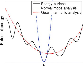
The derivation of normal mode analysis assumes that the system is at a potential energy minimum (so that dU/dx_i=0 and d²U/dx_idx_j>0 for each i and j) (Brooks & Karplus, Reference Brooks and Karplus1983; Brooks et al. Reference Brooks, Janezic and Karplus1995; Wilson et al. Reference Wilson, Decius and Cross1955), thus it is imperative that a system be energy minimized before analysis or else non-physical negative modes will be recovered. Normal mode analysis is relatively inexpensive, as dynamics are not required, but this results in the computed entropy reflecting only the (small) region of phase space surrounding the energy minimum considered (see Fig. 4).

Through the introduction of dynamics, quasi-harmonic analysis attempts to determine an effective potential from the states sampled in a simulation by fitting the observed probability distribution along a degree of freedom to a Gaussian (as would result from a harmonic potential along that coordinate) (Karplus & Kushick, Reference Karplus and Kushick1981; Levy et al. Reference Levy, Karplus, Kushick and Perahia1984). The key difference from normal mode analysis is that the matrix F is constructed from the covariance matrix, which describes the fluctuations in a simulation of each Cartesian coordinate relative to it average:

(31)

$\eqalign{\tab F_{ij} \equals kT\lsqb \sigma \rsqb _{ij} \comma \cr \tab \sigma _{ij} \equals \langle {( {x_{i} \minus \langle {x_{i} }\rangle })}\rangle\langle {( {x_{j} \minus \langle {x_{j} } \rangle })}\rangle \comma \cr}$

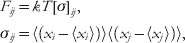
where (x_i) is the average value of x_i throughout the simulation. This results in frequencies which represent a larger range of phase space than in normal mode analysis, as shown in Fig. 4.

Since it relies on extensive phase space sampling, convergence of quasi-harmonic calculations is often obtained only with extensive simulations (Baron et al. Reference Baron, van Gunsteren and Hunenberger2006; Harris et al. Reference Harris, Gavathiotis, Searle, Orozco and Laughton2001). Even with an infinitely long simulation, the quasi-harmonic approximation will only give an upper-bound to the absolute entropy due to the effects of two key assumptions: the harmonic assumptions and the correlations between probability distributions. It has recently been shown that the effects of anharmonicity are relatively small and only affect the lowest few frequencies (Baron et al. Reference Baron, Hunenberger and McCammon2009; Chang et al. Reference Chang, Chen and Gilson2005). In contrast, the correlations between modes may be quite significant. Corrections for both of these have been proposed, but they too are quite expensive and require significant sampling such that corrections beyond pairwise may be computationally infeasible (Baron et al. Reference Baron, Hunenberger and McCammon2009). Despite these drawbacks, the quasi-harmonic approximation has become a powerful method for the estimation of absolute entropies in biomolecular systems.

Fig. 4.

Estimation of effective harmonic potentials U _eff to fit the underlying potential energy surface with a normal mode and quasi-harmonic analysis. The normal mode analysis computes an effective potential based on the landscape local to a minimum energy structure, whereas quasi-harmonic analysis fits an effective potential to the area sampled through a simulation.

4. Interesting results

The methods discussed in the previous section have been extensively utilized throughout the literature in the past three decades. To demonstrate some of their strengths, we present selected results that shed light on the thermodynamic basis of biomolecular recognition. We first address the role configurational entropy plays, and in particular how it relates to the oft discussed ‘entropy/enthalpy compensation’ phenomena. We leave the discussion of solvent entropies to the second part, where the general role of solvent is described. Finally, we present a brief historical view for simulations performed on the model T4 lysozyme system to show not only the evolution of these methods but also their strengths and weaknesses.

4.1 Configurational entropy in biomolecular recognition

Molecular flexibility, which may be thermodynamically quantified as conformational entropy, plays an important role in the thermodynamics of biomolecular recognition. Oftentimes it is observed that the free energy change upon binding can be decomposed into an enthalpic term which favors binding and entropic terms that oppose it. This phenomenon of entropy–enthalpy compensation has been widely discussed in both the experimental and theoretical literature (Baron & McCammon, Reference Baron and McCammon2008; Gallicchio et al. Reference Gallicchio, Kubo and Levy2000; Levy & Gallicchio, Reference Levy and Gallicchio1998; Lumry & Rajender, Reference Lumry and Rajender1970; Olsson et al. Reference Olsson, Williams, Pitt and Ladbury2008; Stone, Reference Stone2001). The physical basis for this is the intuitive idea that the tighter two molecules bind to one another (higher enthalpic interaction), the more restricted their motions are, which results in a lower configurational entropy of the complex. However, the origin of these restricted motions is not entirely clear. For a small host–guest system, mining minima results showed that, counter to what one may expect, binding does not significantly reduce the number of states accessible to the bound system relative to the free one, rather it reduces the motions within these states (Chang & Gilson, Reference Chang and Gilson2004; Chen et al. Reference Chen, Chang and Gilson2004). In contrast, quasi-harmonic calculations on long timescale simulations of the major urinary protein binding to 2-methoxy-3-iosbutylpyrazine showed little change in the protein's or ligand's configurational entropy upon binding (restrictions of motions in one region were offset by increased motion in another), with the only entropic penalty resulting from a loss of rotational degrees of freedom (Roy & Laughton, Reference Roy and Laughton2010). Clearly, the nature and degree of entropic penalties are highly complex and system dependent, but their presences play a key role in biomolecular recognition.

The role of conformational entropy opposing complex formation is believed to be common in nature, but it is by no means a requirement of thermodynamics (Gallicchio et al. Reference Gallicchio, Kubo and Levy1998; Zidek et al. Reference Zidek, Novotny and Stone1999). In fact, some binding interfaces, such as that between protein kinase A (PKA) and any of the numerous A-kinase-anchoring proteins (AKAPs) it binds to, have evolved such that there is an increase in configurational entropy upon binding which aids in stabilizing the complex (Colledge & Scott, Reference Colledge and Scott1999; Fayos et al. Reference Fayos, Melacini, Newlon, Burns, Scott and Jennings2003). Simulations of the PKA D/D domains in complex with the binding peptide from one AKAP, Ht31, demonstrated an increase in side-chain flexibility upon binding relative to the free state (Chang et al. Reference Chang, McLaughlin, Baron, Wang and McCammon2008). It is believed that, when free in solution, the hydrophobic side chains of Ht31 were limited to forming intramolecular contacts, but when bound to PKA the hydrophobic environment of the protein surface creates a fluid-like region that allows for an increase in the number of states accessible to the side chains, and hence an increased entropy. This mechanism may help explain the promiscuous nature of PKA, as its interaction with diverse protein partners may be stabilized through non-specific hydrophobic contacts.

4.2 The role of solvent

Much of the focus on biomolecular recognition is, quite rightly, concerned with the interactions between the solute molecules of interest. However, statistical mechanics does not partition a system into components (such as ‘protein, ‘ligand’ and ‘solvent’); rather, the partition function is a function of the system's Hamiltonian (see Eq. (13)). Therefore, a complete understanding of biomolecular recognition requires consideration of the solvent as well. Two models for the role of solvent exist: it may play a passive role, filling space and screening electrostatics, or it may play a more active role, such as stabilizing biomolecular complexes through interactions with solute molecules. Increasingly it is becoming clear that the latter is often the case.

Oftentimes, individual water molecules play crucial roles in stabilizing biomolecular complexes. Using TI, Hamelberg et al. calculated the binding free energies associated with water molecules directly stabilizing protein–ligand interactions for two complexes, trypsin bound to benzylamine and HIV-1 protease bound to the inhibitor KNI-272 (Hamelberg & McCammon, Reference Hamelberg and McCammon2004). These individual water molecules were shown to contribute 2–3 kcal/mol in free energy to the complex. Using the same technique, Samsonov et al. examined the role of water molecules in stabilizing protein–protein interactions, and showed that water molecules have diverse roles in mediating protein contacts (Samsonov et al. Reference Samsonov, Teyra and Pisabarro2008). In one case it was shown that hydrogen bonds between two water molecules resulted in cooperative stabilization of protein interactions, indicating that complex interaction dynamics between multiple solvent molecules and solute sites may be important for providing a complete understanding of recognition processes.

The heterogeneous roles of solvent molecules in biomolecular recognition have made it difficult to discern general principles describing water interactions. Recent simulations on a model system addressed this question. Through the use of umbrella sampling calculations at multiple temperatures on the simple model system of a spherical ligand binding into a hemispherical cavity, Baron et al. decomposed the entropic and enthalpic contributions to ligand binding or rejection for neutral and charged ligands binding to neutral and charged receptors (Baron et al. Reference Baron, Setny and McCammon2010; Hummer, Reference Hummer2010; Setny et al. Reference Setny, Baron and McCammon2010). Results demonstrated that water dominated the binding thermodynamics. Surprisingly, the hydrophobic binding of a neutral ligand to a neutral receptor was found to be more stable than that of a charged ligand to an oppositely charged receptor. This hydrophobic association is enthalpically driven due to the increased number of water–water hydrogen bonds when the ligand is bound in the receptor, since in the unbound state water molecules must occupy the receptor and are forced into geometries that are sub-optimal for hydrogen bonding with neighboring water molecules. The polarity of the water molecules also resulted in a charge asymmetry, with a positively charged ligand binding stronger to a negative receptor than a negatively charged ligand binding to a positive receptor, largely due to increased entropic costs in the latter case which are not prevalent in the former.

The increased focus on individual water molecules in biomolecular recognition has led to the development of new tools to aid in addressing their thermodynamics. Two recent tools, JAWS and WaterMap, attempt to address this by using grand canonical Monte Carlo and explicit-solvent MD simulations, respectively, to compute the ‘hydration sites’ (regions with high-water density) in a protein's binding site, along with the thermodynamics of expulsion of a water molecule in that site to the bulk solvent (Abel et al. Reference Abel, Young, Farid, Berne and Friesner2008, Reference Abel, Wang, Friesner and Berne2010; Michel et al. Reference Michel, Tirado-Rives and Jorgensen2009b; Young et al. Reference Young, Abel, Kim, Berne and Friesner2007). This free energy difference dictates whether displacement of the water molecule by a ligand is thermodynamically favorable or not, and early results indicate that, for a congeneric series of ligands, the correlation between these scores and experimental binding energies is quite good, suggesting that this is a fundamentally important component in the thermodynamics of protein–ligand interaction which may not have been accurately accounted for in the past (Beuming et al. Reference Beuming, Farid and Sherman2009; Guimãraes & Mathiowetz, Reference Guimãraes and Mathiowetz2010; Michel et al. Reference Michel, Tirado-Rives and Jorgensen2009b; Pearlstein et al. Reference Pearlstein, Hu, Zhou, Yowe, Levell, Dale, Kaushik, Daniels, Hanrahan, Sherman and Abel2010). However, because these methods do not directly account for protein–ligand interactions, they may only be expected to perform well for ligands that form a near-optimal number of polar and apolar contacts with the host protein.

4.3 The case of T4 lysozyme

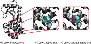
The association of a ligand into a protein's binding site is not only conceptually more straightforward than protein–protein recognition, it has obvious pharmaceutical implications. Therefore, it is not surprising that a majority of work in the field has gone towards the development of methods to predict both the binding configurations and energies of small molecules in protein binding sites. To effectively advance these methods, model systems are required which may be easily studied by both experimental and computational techniques. The T4 lysozyme has become one of these systems (Wei et al. Reference Wei, Baase, Weaver, Matthews and Shoichet2002). Mutation of a leucine to an alanine at position 99 creates a cavity that is small, hydrophobic, and free from solvent interactions, thus creating a simple binding site for small, apolar ligands (see Fig. 5a, b) (Eriksson et al. Reference Eriksson, Baase, Wozniak and Matthews1992; Morton & Matthews, Reference Morton and Matthews1995; Morton et al. Reference Morton, Baase and Matthews1995). A single hydrogen bond acceptor can be introduced into this cavity through the mutation of the methionine at position 102 to glutamine (the L99A/M102Q mutant), creating a model site that preferentially binds small molecules that have one or two hydrogen bond donors (see Fig. 5c) (Boyce et al. Reference Boyce, Mobley, Rocklin, Graves, Dill and Shoichet2009). Here, we present a brief overview of some of the applications of the free energy methods described above, and their limitations, to both of these model binding sites.

Fig. 5.

Structure of the L99A mutant of T4 lysozyme with a benzene molecule bound in the non-polar binding site (PDB ID: 181L, Morton & Matthews, Reference Morton and Matthews1995) (a, b), and the polar L99A/M102Q mutant with a bound catechol molecule (PDB ID: 1XEP, Graves et al. Reference Graves, Brenk and Shoichet2005) (c). These two mutants have become model systems upon which numerous computational studies have been performed. Side chains for residues Val111 and Met102 (Gln102 in (c)) are shown.

Hermans and Wang provided an early example of applying alchemical transformation methods to protein–ligand interactions with their calculations of the binding energy for benzene in the L99A cavity (Hermans & Wang, Reference Hermans and Wang1997). Although computational power limited their simulation length (relative to modern simulations), calculations with mobile protein atoms that were initiated from the L99A/benzene crystal structure showed remarkably good agreement with experimental binding energies (−5.14 kcal/mol versus −5.19 kcal/mol). The importance of receptor flexibility and the initial configuration was highlighted in a series of simulations in which the protein was held rigid in various conformations, resulting in inaccurate free energies varying from −3.5 to −8.9 kcal/mol. In a subsequent study, Mann and Hermans used similar technique (with longer simulation times) to analyze the binding of noble gases into the L99A binding pocket, with results agreeing well with crystallographic data for binding site locations and occupancy thermodynamics of xenon, argon and krypton ions at high pressure (Mann & Hermans, Reference Mann and Hermans2000). The longer simulations also allowed for the observation of large and slow interdomain motions, while intradomain structures were relatively rigid, consistent with previous MD simulations (de Groot et al. Reference de Groot, Hayward, van Aalten, Amadei and Berendsen1998; Hayward & Berendsen, Reference Hayward and Berendsen1998).

As free energy methods have developed, T4 lysozyme has been used to test their effectiveness, such as in the introduction of restraint potentials necessary for ensuring that the species being decoupled in alchemical transformations retains pertinent locations and orientations (Boresch et al. Reference Boresch, Tettinger, Leitgeb and Karplus2003; Deng & Roux, Reference Deng and Roux2006). Mobley et al. focused on testing alchemical methods in the pharmaceutically relevant context of predicting highly accurate binding affinities for a series of small molecules to a specific binding site (Mobley et al. Reference Mobley, Chodera and Dill2007 Reference Mobley, Graves, Chodera, McReynolds, Shoichet and Dillb). First, they examined the binding of 13 aromatic molecules into the binding cavity of L99A, 11 of which ITC experiments had previously established binding affinities for, and two of which were known to be non-binders. When only a single initial configuration was accounted for, calculations showed a root mean square (RMS) error of 3.51 kcal/mol and a correlation, R, of 0.51 to experimental values. These values could be improved to 2.55 kcal/mol and 0.72 by including multiple initial configurations. The authors noted the side chain of valine 111 reoriented upon binding in crystal structures but not in their simulations (due to high energy barriers), and achieved improved agreement to experiments (2.24 kcal/mol and R=0.72) by forcing rotation of this side chain using the ‘confine-and-release’ method (Mobley et al. Reference Mobley, Chodera and Dill2007a). Their best agreement to experimental values came upon replacement of the charge model of the ligands with a model closer to the one used in parameterizing the protein, for a final RMS of 1.89 kcal/mol and R=0.79. The group then used this method on a blind test of five small molecules predicted to bind with docking algorithms while subsequently experimentally determining their docking poses with X-ray crystallography and binding affinities by ITC. Not only did the free energy calculations provide docking poses close to the experimentally observed ones, they correctly discriminated between binders and non-binders and had an RMS error of only 0.57 kcal/mol, both of which were substantial improvements upon docking results.

In a follow up study by the same groups, Boyce et al. performed similar blind tests on the polar cavity of the L99A/M102Q mutant and showed that the inclusion of polarity reduced the reliability of alchemical calculations (Boyce et al. Reference Boyce, Mobley, Rocklin, Graves, Dill and Shoichet2009). In this work, 13 small molecules were tested, yielding correct predictions on the binary question of whether a molecule would bind or not for 10 of these. The RMS error to experiments was 1.8 kcal/mol (excluding the non-binders for which affinity could not be measured), and the rank ordering of ligands did not agree with experiments. Relative free energies within congeneric series were also calculated, and it was shown that the reliability of free energies within a series was related to the accuracy of the ligand poses. For the best series (modifications of the ligand catechol), the RMS error was only 1.1 kcal/mol and the rank ordering of modifications agreed with experiments. It is worth noting that results for both this site and the L99A cavity were much improved (although more expensive) over end-point calculations using MM-GBSA calculations, which had difficulty discerning between binders and non-binders (Graves et al. Reference Graves, Shivakumar, Boyce, Jacobson, Case and Shoichet2008).

5. Conclusion

Through the use of methods grounded in statistical mechanics, computer simulations have proved invaluable in advancing our understanding of thermodynamic properties important in biomolecular recognition. Thermodynamic pathway calculations, while expensive, provide the best agreement to experimental free energy results, with errors typically of the order of 1–2 kcal/mol, while quicker end-point calculations provide a decent approximation with higher errors. Harmonic and quasi-harmonic calculations may be used to compute the conformational entropy of a protein through the use of either static structures or simulation results. The refinement of these techniques and the development of new ones show promise for improving our ability to calculate thermodynamics with increased precision. These simulations should be viewed as a complement to experimental methods, and as both the methods and the computing power increase so too should our ability to interpret and guide future experiments.

6. Acknowledgements

We thank R. Baron, M. Fajer, P. Gasper, M. Lawrenz, S. Nichols and Y. Wang for comments about this manuscript. Support for this review was provided by Award Number F32GM093581 from the National Institute of General Medical Sciences. Additional support has been provided by the National Science Foundation, the National Institutes of Health, the Howard Hughes Medical Institute, the Center for Theoretical Biological Physics, the National Biomedical Computation Resource and the NSF Teragrid project.

References

7. References

Abel, R., Wang, L. L., Friesner, R. A. & Berne, B. J. (2010). A displaced-solvent functional analysis of model hydrophobic enclosures. Journal of Chemical Theory and Computation 6, 2924–2934.CrossRef Google Scholar PubMed

Abel, R., Young, T., Farid, R., Berne, B. J. & Friesner, R. A. (2008). Role of the active-site solvent in the thermodynamics of factor Xa ligand binding. Journal of the American Chemical Society 130, 2817–2831.CrossRef Google Scholar PubMed

Adcock, S. A. & McCammon, J. A. (2006). Molecular dynamics: survey of methods for simulating the activity of proteins. Chemical Reviews 106, 1589–1615.CrossRef Google Scholar PubMed

Andricioaei, I. & Karplus, M. (2001). On the calculation of entropy from covariance matrices of the atomic fluctuations. Journal of Chemical Physics 115, 6289–6292.CrossRef Google Scholar

Baron, R., Hunenberger, P. H. & McCammon, J. A. (2009). Absolute single-molecule entropies from quasi-harmonic analysis of microsecond molecular dynamics: correction terms and convergence properties. Journal of Chemical Theory and Computation 5, 3150–3160.CrossRef Google Scholar PubMed

Baron, R. & McCammon, J. A. (2008). (Thermo)dynamic role of receptor flexibility, entropy, and motional correlation in protein-ligand binding. ChemPhysChem 9, 983–988.CrossRef Google Scholar PubMed

Baron, R., Setny, P. & McCammon, J. A. (2010). Water in cavity-ligand recognition. Journal of the American Chemical Society 132, 12091–12097.CrossRef Google Scholar PubMed

Baron, R., van Gunsteren, W. F. & Hunenberger, P. H. (2006). Estimating the configurational entropy from molecular dynamics simulations: anharmonicity and correlation corrections to the quasi-harmonic approximation. Trends in Physical Chemistry 11, 87–122.Google Scholar

Barril, X., Gelpi, J. L., Lopez, J. M., Orozco, M. & Luque, F. J. (2001). How accurate can molecular dynamics/linear response and Poisson–Boltzmann/solvent accessible surface calculations be for predicting relative binding affinities? Acetylcholinesterase huprine inhibitors as a test case. Theoretical Chemistry Accounts 106, 2–9.CrossRef Google Scholar

Best, R. B., Buchete, N. V. & Hummer, G. (2008). Are current molecular dynamics force fields too helical? Biophysical Journal 95, L7–L9.CrossRef Google Scholar PubMed

Beuming, T., Farid, R. & Sherman, W. (2009). High-energy water sites determine peptide binding affinity and specificity of PDZ domains. Protein Science 18, 1609–1619.CrossRef Google Scholar PubMed

Beutler, T. C. & van Gunsteren, W. F. (1994). Molecular-dynamics free-energy calculation in 4 dimensions. Journal of Chemical Physics 101, 1417–1422.CrossRef Google Scholar

Beutler, T. C., Mark, A. E., Vanschaik, R. C., Gerber, P. R. & van Gunsteren, W. F. (1994). Avoiding singularities and numerical instabilities in free-energy calculations based on molecular simulations. Chemical Physics Letters 222, 529–539.CrossRef Google Scholar

Boresch, S., Tettinger, F., Leitgeb, M. & Karplus, M. (2003). Absolute binding free energies: a quantitative approach for their calculation. Journal of Physical Chemistry B 107, 9535–9551.CrossRef Google Scholar

Boyce, S. E., Mobley, D. L., Rocklin, G. J., Graves, A. P., Dill, K. A. & Shoichet, B. K. (2009). Predicting ligand binding affinity with alchemical free energy methods in a polar model binding site. Journal of Molecular Biology 394, 747–763.CrossRef Google Scholar

Brooijmans, N. & Kuntz, I. D. (2003). Molecular recognition and docking algorithms. Annual Review of Biophysics and Biomolecular Structure 32, 335–373.CrossRef Google Scholar PubMed

Brooks, B. & Karplus, M. (1983). Harmonic dynamics of proteins-normal-modes and fluctuations in bovine pancreatic trypsin-inhibitor. Proceedings of the National Academy of Sciences of the United States of America 80, 6571–6575.CrossRef Google Scholar PubMed

Brooks, B. R., Janezic, D. & Karplus, M. (1995). Harmonic-analysis of large systems. 1. Methodology. Journal of Computational Chemistry 16, 1522–1542.CrossRef Google Scholar

Carlsson, J. & Åqvist, J. (2005). Absolute and relative entropies from computer simulation with applications to ligand binding. Journal of Physical Chemistry B 109, 6448–6456.CrossRef Google Scholar PubMed

Carlsson, J. & Åqvist, J. (2006). Calculations of solute and solvent entropies from molecular dynamics simulations. Physical Chemistry Chemical Physics 8, 5385–5395.CrossRef Google Scholar PubMed

Chandler, D. (1987). Introduction to Modern Statistical Mechanics. New York: Oxford University.Google Scholar

Chang, C. E. & Gilson, M. K. (2004). Free energy, entropy, and induced fit in host-guest recognition: calculations with the second-generation mining minima algorithm. Journal of the American Chemical Society 126, 13156–13164.CrossRef Google Scholar PubMed

Chang, C. E., Chen, W. & Gilson, M. K. (2005). Evaluating the accuracy of the quasiharmonic approximation. Journal of Chemical Theory and Computation 1, 1017–1028.CrossRef Google Scholar PubMed

Chang, C. E. A., McLaughlin, W. A., Baron, R., Wang, W. & McCammon, J. A. (2008). Entropic contributions and the influence of the hydrophobic environment in promiscuous protein-protein association. Proceedings of the National Academy of Sciences of the United States of America 105, 7456–7461.Google Scholar

Chen, W., Chang, C. E. & Gilson, M. K. (2004). Calculation of cyclodextrin binding affinities: energy, entropy, and implications for drug design. Biophysical Journal 87, 3035–3049.CrossRef Google Scholar PubMed

Chen, W., Gilson, M. K., Webb, S. P. & Potter, M. J. (2010). Modeling protein-ligand binding by mining minima. Journal of Chemical Theory and Computation 6, 3540–3557.CrossRef Google Scholar PubMed

Chipot, C. & Pohorille, A. (2007). Free Energy Calculations. Berlin: Springer.CrossRef Google Scholar

Christ, C. D. & van Gunsteren, W. F. (2007). Enveloping distribution sampling: a method to calculate free energy differences from a single simulation. Journal of Chemical Physics 126, 184110.CrossRef Google Scholar PubMed

Christ, C. D. & van Gunsteren, W. F. (2008). Multiple free energies from a single simulation: extending enveloping distribution sampling to nonoverlapping phase-space distributions. Journal of Chemical Physics 128, 174112.CrossRef Google Scholar PubMed

Colledge, M. & Scott, J. D. (1999). AKAPs: from structure to function. Trends in Cell Biology 9, 216–221.CrossRef Google Scholar PubMed

Darve, E., Rodriguez-Gomez, D. & Pohorille, A. (2008). Adaptive biasing force method for scalar and vector free energy calculations. Journal of Chemical Physics 128, 144120.Google Scholar

de Groot, B. L., Hayward, S., van Aalten, D. M. F., Amadei, A. & Berendsen, H. J. C. (1998). Domain motions in bacteriophage T4 lysozyme: a comparison between molecular dynamics and crystallographic data. Proteins-Structure Function and Genetics 31, 116–127.3.0.CO;2-K>CrossRef Google Scholar PubMed

Deng, Y. Q. & Roux, B. (2006). Calculation of standard binding free energies: aromatic molecules in the T4 lysozyme L99A mutant. Journal of Chemical Theory and Computation 2, 1255–1273.CrossRef Google Scholar PubMed

Durrant, J. D. & McCammon, J. A. (2010). Computer-aided drug-discovery techniques that account for receptor flexibility. Current Opinion In Pharmacology 10, 770–774.CrossRef Google Scholar PubMed

Eriksson, A. E., Baase, W. A., Wozniak, J. A. & Matthews, B. W. (1992). A cavity-containing mutant of T4 lysozyme is stabilized by buried benzene. Nature 355, 371–373.CrossRef Google Scholar PubMed

Fajer, M., Hamelberg, D. & McCammon, J. A. (2008). Replica-exchange accelerated molecular dynamics (REXAMD) applied to thermodynamic integration. Journal of Chemical Theory and Computation 4, 1565–1569.CrossRef Google Scholar PubMed

Fayos, R., Melacini, G., Newlon, M. G., Burns, L., Scott, J. D. & Jennings, P. A. (2003). Induction of flexibility through protein–protein interactions. Journal of Biological Chemistry 278, 18581–18587.CrossRef Google Scholar PubMed

Fuentes, G., Dastidar, S. G., Madhumalar, A. & Verma, C. S. (2011). Role of protein flexibility in the discovery of new drugs. Drug Development Research 72, 26–35.CrossRef Google Scholar

Gallicchio, E., Kubo, M. M. & Levy, R. M. (1998). Entropy-enthalpy compensation in solvation and ligand binding revisited. Journal of the American Chemical Society 120, 4526–4527.Google Scholar

Gallicchio, E., Kubo, M. M. & Levy, R. M. (2000). Enthalpy-entropy and cavity decomposition of alkane hydration free energies: numerical results and implications for theories of hydrophobic solvation. Journal of Physical Chemistry B 104, 6271–6285.CrossRef Google Scholar

Gellman, S. H. (1997). Molecular recognition. Chemical Reviews 97, 1231–1734.CrossRef Google Scholar PubMed

Gilson, M. K. & Honig, B. (1988). Calculation of the total electrostatic energy of a macromolecular system: solvation energies, binding energies, and conformational analysis. Proteins: Structure Function and Bioinformatics 4, 7–18.CrossRef Google Scholar PubMed

Gilson, M. K. & Zhou, H. X. (2007). Calculation of protein-ligand binding affinities. Annual Review of Biophysics and Biomolecular Structure 36, 21–42.CrossRef Google Scholar PubMed

Gilson, M. K., Given, J. A., Bush, B. L. & McCammon, J. A. (1997a). The statistical-thermodynamic basis for computation of binding affinities: a critical review. Biophysical Journal 72, 1047–1069.CrossRef Google Scholar PubMed

Gilson, M. K., Given, J. A. & Head, M. S. (1997b). A new class of models for computing receptor-ligand binding affinities. Chemistry and Biology 4, 87–92.CrossRef Google Scholar PubMed

Graves, A. P., Brenk, R. & Shoichet, B. K. (2005). Decoys for docking. Journal of Medicinal Chemistry 48, 3714–3728.CrossRef Google Scholar PubMed

Graves, A. P., Shivakumar, D. M., Boyce, S. E., Jacobson, M. P., Case, D. A. & Shoichet, B. K. (2008). Rescoring docking hit lists for model cavity sites: predictions and experimental testing. Journal of Molecular Biology 377, 914–934.CrossRef Google Scholar PubMed

Guimaraes, C. R. W. & Cardozo, M. (2008). MM-GB/SA rescoring of docking poses in structure-based lead optimization. Journal of Chemical Information and Modeling 48, 958–970.CrossRef Google Scholar PubMed

Guimãraes, C. R. W. & Mathiowetz, A. M. (2010). Addressing limitations with the MMGB/SA scoring procedure using the water map method and free energy perturbation calculations. Journal of Chemical Information and Modeling 50, 547–559.Google Scholar

Guvench, O. & MacKerell, A. D. (2009). Computational evaluation of protein-small molecule binding. Current Opinion in Structural Biology 19, 56–61.CrossRef Google Scholar PubMed

Halperin, I., Ma, B. Y., Wolfson, H. & Nussinov, R. (2002). Principles of docking: an overview of search algorithms and a guide to scoring functions. Proteins: Structure Function and Genetics 47, 409–443.CrossRef Google Scholar

Hamelberg, D. & McCammon, J. A. (2004). Standard free energy of releasing a localized water molecule from the binding pockets of proteins: double-decoupling method. Journal of the American Chemical Society 126, 7683–7689.CrossRef Google Scholar PubMed

Hamelberg, D., Mongan, J. & McCammon, J. A. (2004). Accelerated molecular dynamics: a promising and efficient simulation method for biomolecules. Journal of Chemical Physics 120, 11919–11929.CrossRef Google Scholar PubMed

Harris, S. A., Gavathiotis, E., Searle, M. S., Orozco, M. & Laughton, C. A. (2001). Cooperativity in drug-DNA recognition: a molecular dynamics study. Journal of the American Chemical Society 123, 12658–12663.CrossRef Google Scholar PubMed

Hayward, S. & Berendsen, H. J. C. (1998). Systematic analysis of domain motions in proteins from conformational change: new results on citrate synthase and T4 lysozyme. Proteins: Structure Function And Genetics 30, 144–154.Google Scholar

Hermans, J. & Wang, L. (1997). Inclusion of loss of translational and rotational freedom in theoretical estimates of free energies of binding. Application to a complex of benzene and mutant T4 lysozyme. Journal of the American Chemical Society 119, 2707–2714.CrossRef Google Scholar

Hummer, G. (2010). Molecular binding under water's influence. Nature Chemistry 2, 906–907.CrossRef Google Scholar PubMed

Jiang, W. & Roux, B. (2010). Free energy perturbation Hamiltonian replica-exchange molecular dynamics (FEP/H-REMD) for absolute ligand binding free energy calculations. Journal of Chemical Theory and Computation 6, 2559–2565.Google Scholar

Jorge, M., Garrido, N. M., Queimada, A. J., Economou, I. G. & Macedo, E. A. (2010). Effect of the integration method on the accuracy and computational efficiency of free energy calculations using thermodynamic integration. Journal of Chemical Theory and Computation 6, 1018–1027.Google Scholar

Karplus, M. & Kushick, J. N. (1981). Method for estimating the configurational entropy of macromolecules. Macromolecules 14, 325–332.CrossRef Google Scholar

Kirkwood, J. G. (1935). Statistical mechanics of fluid mixtures. Journal of Chemical Physics 3, 300–313.CrossRef Google Scholar

Kitchen, D. B., Decornez, H., Furr, J. R. & Bajorath, J. (2004). Docking and scoring in virtual screening for drug discovery: methods and applications. Nature Reviews Drug Discovery 3, 935–949.Google Scholar

Klebe, G. (2006). Virtual ligand screening: strategies, perspectives and limitations. Drug Discovery Today 11, 580–594.Google Scholar

Knight, J. L. & Brooks, C. L. (2009). λ-dynamics free energy simulation methods. Journal of Computational Chemistry 30, 1692–1700.CrossRef Google Scholar PubMed

Kollman, P. A., Massova, I., Reyes, C., Kuhn, B., Huo, S. H., Chong, L., Lee, M., Lee, T., Duan, Y., Wang, W., Donini, O., Cieplak, P., Srinivasan, J., Case, D. A. & Cheatham, T. E. (2000). Calculating structures and free energies of complex molecules: combining molecular mechanics and continuum models. Accounts of Chemical Research 33, 889–897.CrossRef Google Scholar PubMed

Kong, X. J. & Brooks, C. L. (1996). λ-dynamics: a new approach to free energy calculations. Journal of Chemical Physics 105, 2414–2423.Google Scholar

Kumar, S., Bouzida, D., Swendsen, R. H., Kollman, P. A. & Rosenberg, J. M. (1992). The weighted histogram analysis method for free-energy calculations on biomolecules .1. The method. Journal of Computational Chemistry 13, 1011–1021.Google Scholar

Ladbury, J. E. & Chowdhry, B. Z. (1996). Sensing the heat: the application of isothermal titration calorimetry to thermodynamic studies of biomolecular interactions. Chemical Biology 3, 791–801.CrossRef Google Scholar PubMed

Laio, A. & Parrinello, M. (2002). Escaping free-energy minima. Proceedings of the National Academy of Sciences of the United States of America 99, 12562–12566.CrossRef Google Scholar PubMed

Lawrenz, M., Baron, R. & McCammon, J. A. (2009). Independent-trajectories thermodynamic-integration free-energy changes for biomolecular systems: determinants of H5N1 avian influenza virus neuraminidase inhibition by peramivir. Journal of Chemical Theory and Computation 5, 1106–1116.Google Scholar

Lee, M. R. & Sun, Y. X. (2007). Improving docking accuracy through molecular mechanics generalized born optimization and scoring. Journal of Chemical Theory and Computation 3, 1106–1119.CrossRef Google Scholar PubMed

Levy, R. M. & Gallicchio, E. (1998). Computer simulations with explicit solvent: recent progress in the thermodynamic decomposition of free energies and in modeling electrostatic effects. Annual Review of Physical Chemistry 49, 531–567.CrossRef Google Scholar PubMed

Levy, R. M., Karplus, M., Kushick, J. & Perahia, D. (1984). Evaluation of the configurational entropy for proteins: application to molecular-dynamics simulations of an α-helix. Macromolecules 17, 1370–1374.Google Scholar

Lumry, R. & Rajender, S. (1970). Enthalpy-entropy compensation phenomena in water solutions of proteins and small molecules: a ubiquitous property of water. Biopolymers 9, 1125–1227.Google Scholar

Lyne, P. D., Lamb, M. L. & Saeh, J. C. (2006). Accurate prediction of the relative potencies of members of a series of kinase inhibitors using molecular docking and MM-GBSA scoring. Journal of Medicinal Chemistry 49, 4805–4808.CrossRef Google Scholar PubMed

Mackerell, A. D. (2004). Empirical force fields for biological macromolecules: overview and issues. Journal of Computational Chemistry 25, 1584–1604.Google Scholar

Mann, G. & Hermans, J. (2000). Modeling protein-small molecule interactions: structure and thermodynamics of noble gases binding in a cavity in mutant phage T4 lysozyme L99A. Journal of Molecular Biology 302, 979–989.CrossRef Google Scholar

McCammon, J. A. (1998). Theory of biomolecular recognition. Current Opinion in Structural Biology 8, 245–249.Google Scholar

Michel, J., Tirado-Rives, J. & Jorgensen, W. L. (2009a). Prediction of the water content in protein binding sites. Journal of Physical Chemistry B 113, 13337–13346.CrossRef Google Scholar PubMed

Michel, J., Tirado-Rives, J. & Jorgensen, W. L. (2009b). Energetics of displacing water molecules from protein binding sites: consequences for ligand optimization. Journal of the American Chemical Society 131, 15403–15411.CrossRef Google Scholar PubMed

Mobley, D. L., Chodera, J. D. & Dill, K. A. (2007a). Confine-and-release method: obtaining correct binding free energies in the presence of protein conformational change. Journal of Chemical Theory and Computation 3, 1231–1235.CrossRef Google Scholar PubMed

Mobley, D. L., Graves, A. P., Chodera, J. D., McReynolds, A. C., Shoichet, B. K. & Dill, K. A. (2007b). Predicting absolute ligand binding free energies to a simple model site. Journal of Molecular Biology 371, 1118–1134.CrossRef Google Scholar PubMed

Morton, A. & Matthews, B. W. (1995). Specificity of ligand-binding in a buried nonpolar cavity of T4 lysozyme-linkage of dynamics and structural plasticity. Biochemistry 34, 8576–8588.CrossRef Google Scholar

Morton, A., Baase, W. A. & Matthews, B. W. (1995). Energetic origins of specificity of ligand-binding in an interior nonpolar cavity of T4 lysozyme. Biochemistry 34, 8564–8575.Google Scholar

Olsson, T. S. G., Williams, M. A., Pitt, W. R. & Ladbury, J. E. (2008). The thermodynamics of protein-ligand interaction and solvation: insights for ligand design. Journal of Molecular Biology 384, 1002–1017.Google Scholar

Oostenbrink, C. & van Gunsteren, W. F. (2003). Single-step perturbations to calculate free energy differences from unphysical reference states: limits on size, flexibility, and character. Journal of Computational Chemistry 24, 1730–1739.Google Scholar

Oostenbrink, C. & van Gunsteren, W. F. (2005). Free energies of ligand binding for structurally diverse compounds. Proceedings of the National Academy of Sciences of the United States of America 102, 6750–6754.Google Scholar

Pearlstein, R. A., Hu, Q. Y., Zhou, J., Yowe, D., Levell, J., Dale, B., Kaushik, V. K., Daniels, D., Hanrahan, S., Sherman, W. & Abel, R. (2010). New hypotheses about the structure-function of proprotein convertase subtilisin/kexin type 9: analysis of the epidermal growth factor-like repeat a docking site using WaterMap. Proteins: Structure Function and Bioinformatics 78, 2571–2586.CrossRef Google Scholar PubMed

Petsko, G. A. & Ringe, D. (1984). Fluctuations in protein-structure from X-ray-diffraction. Annual Review of Biophysics and Bioengineering 13, 331–371.CrossRef Google Scholar PubMed

Rodinger, T., Howell, P. L. & Pomes, R. (2005). Absolute free energy calculations by thermodynamic integration in four spatial dimensions. Journal of Chemical Physics 123, 034104.CrossRef Google Scholar PubMed

Roux, B. (1995). The calculation of the potential of mean force using computer-simulations. Computer Physics Communications 91, 275–282.CrossRef Google Scholar

Roy, J. & Laughton, C. A. (2010). Long-timescale molecular-dynamics simulations of the major urinary protein provide atomistic interpretations of the unusual thermodynamics of ligand binding. Biophysical Journal 99, 218–226.Google Scholar

Samsonov, S., Teyra, J. & Pisabarro, T. (2008). A molecular dynamics approach to study the importance of solvent in protein interactions. Proteins: Structure Function and Bioinformatics 73, 515–525.Google Scholar

Setny, P., Baron, R. & McCammon, J. A. (2010). How can hydrophobic association be enthalpy driven? Journal of Chemical Theory and Computation 6, 2866–2871.Google Scholar

Shaw, D. E., Deneroff, M. M., Dror, R. O., Kuskin, J. S., Larson, R. H., Salmon, J. K., Young, C., Batson, B., Bowers, K. J., Chao, J. C., Eastwood, M. P., Gagliardo, J., Grossman, J. P., Ho, C. R., Ierardi, D. J., Kolossváry, I., Klepeis, J. L., Layman, T., McLeavey, C., Moraes, M. A., Mueller, R., Priest, E. C., Shan, Y., Spengler, J., Theobald, M., Towles, B. & Wang, S. C. (2008). Anton, a special-purpose machine for molecular dynamics simulation. Communications of the ACM 51, 91–97.CrossRef Google Scholar

Shirts, M. R. & Chodera, J. D. (2008). Statistically optimal analysis of samples from multiple equilibrium states. Journal of Chemical Physics 129, 124105.Google Scholar

Shirts, M. R. & Pande, V. S. (2005). Comparison of efficiency and bias of free energies computed by exponential averaging, the Bennett acceptance ratio, and thermodynamic integration. Journal of Chemical Physics 122, 144107.Google Scholar

Shirts, M. R., Bair, E., Hooker, G. & Pande, V. S. (2003). Equilibrium free energies from nonequilibrium measurements using maximum-likelihood methods. Physical Review Letters 91, 140601.CrossRef Google Scholar PubMed

Shirts, M. R., Mobley, D. L. & Chodera, J. D. (2007). Alchemical free energy calculations: ready for prime time? Annual Reports in Computational Chemistry 3, 41–59.Google Scholar

Sitkoff, D., Sharp, K. & Honig, B. (1994). Accurate calculation of hydration free energies using macroscopic solvent models. Journal of Physical Chemistry 98, 1978–1988.Google Scholar

Srinivasan, J., Cheatham, T. E., Cieplak, P., Kollman, P. A. & Case, D. A. (1998). Continuum solvent studies of the stability of DNA, RNA, and phosphoramidate-DNA helices. Journal of the American Chemical Society 120, 9401–9409.CrossRef Google Scholar

Still, W. C., Tempczyk, A., Hawley, R. C. & Hendrickson, T. (1990). Semianalytical treatment of solvation for molecular mechanics and dynamics. Journal of the American Chemical Society 112, 6127–6129.Google Scholar

Stone, J. E., Phillips, J. C., Freddolino, P. L., Hardy, D. J., Trabuco, L. G. & Schulten, K. (2007). Accelerating molecular modeling applications with graphics processors. Journal of Computational Chemistry 28, 2618–2640.Google Scholar

Stone, M. J. (2001). NMR relaxation studies of the role of conformational entropy in protein stability and ligand binding. Accounts of Chemical Research 34, 379–388.CrossRef Google Scholar PubMed

Straatsma, T. P. & McCammon, J. A. (1991). Multiconfiguration thermodynamic integration. Journal of Chemical Physics 95, 1175–1188.CrossRef Google Scholar

Straatsma, T. P. & McCammon, J. A. (1992). Computational alchemy. Annual Review of Physical Chemistry 43, 407–435.Google Scholar

Swanson, J. M. J., Henchman, R. H. & McCammon, J. A. (2004). Revisiting free energy calculations: a theoretical connection to MM/PBSA and direct calculation of the association free energy. Biophysical Journal 86, 67–74.Google Scholar

Thomas, A. S. & Elcock, A. H. (2006). Direct observation of salt effects on molecular interactions through explicit-solvent molecular dynamics simulations: differential effects on electrostatic and hydrophobic interactions and comparisons to Poisson-Boltzmann theory. Journal of the American Chemical Society 128, 7796–7806.CrossRef Google Scholar PubMed

Toda, M., Kubo, R. & Saitô, (1992). Statistical Physics I. Berlin: Springer.Google Scholar

Torrie, G. M. & Valleau, J. P. (1977). Non-physical sampling distributions in Monte-Carlo free-energy estimation – umbrella sampling. Journal of Computational Physics 23, 187–199.Google Scholar

Wang, J. M., Morin, P., Wang, W. & Kollman, P. A. (2001). Use of MM-PBSA in reproducing the binding free energies to HIV-1 RT of TIBO derivatives and predicting the binding mode to HIV-1 RT of efavirenz by docking and MM-PBSA. Journal of the American Chemical Society 123, 5221–5230.CrossRef Google Scholar PubMed

Wang, J. Y., Deng, Y. Q. & Roux, B. (2006). Absolute binding free energy calculations using molecular dynamics simulations with restraining potentials. Biophysical Journal 91, 2798–2814.Google Scholar

Wei, B. Q. Q., Baase, W. A., Weaver, L. H., Matthews, B. W. & Shoichet, B. K. (2002). A model binding site for testing scoring functions in molecular docking. Journal of Molecular Biology 322, 339–355.CrossRef Google Scholar

Weis, A., Katebzadeh, K., Soderhjelm, P., Nilsson, I. & Ryde, U. (2006). Ligand affinities predicted with the MM/PBSA method: dependence on the simulation method and the force field. Journal of Medicinal Chemistry 49, 6596–6606.CrossRef Google Scholar PubMed

Wereszczynski, J. & McCammon, J. A. (2010). Using selectively applied accelerated molecular dynamics to enhance free energy calculations. Journal of Chemical Theory and Computation 6, 3285–3293.CrossRef Google Scholar PubMed

Wilson, E. B., Decius, J. C. & Cross, P. C. (1955). Molecular Vibrations. New York: McGraw-Hill.Google Scholar

Woods, C. J., Essex, J. W. & King, M. A. (2003). The development of replica-exchange based free-energy methods. Journal of Physical Chemistry B 107, 13703–13710.Google Scholar

Young, T., Abel, R., Kim, B., Berne, B. J. & Friesner, R. A. (2007). Motifs for molecular recognition exploiting hydrophobic enclosure in protein-ligand binding. Proceedings of the National Academy of Sciences of the United States of America 104, 808–813.Google Scholar

Zacharias, M., Straatsma, T. P. & McCammon, J. A. (1994). Separation-shifted scaling, a new scaling method for Lennard–Jones interactions in thermodynamic integration. Journal of Chemical Physics 100, 9025–9031.Google Scholar

Zhou, H. X. & Gilson, M. K. (2009). Theory of free energy and entropy in noncovalent binding. Chemical Reviews 109, 4092–4107.Google Scholar

Zidek, L., Novotny, M. V. & Stone, M. J. (1999). Increased protein backbone conformational entropy upon hydrophobic ligand binding. Nature Structural Biology 6, 1118–1121.Google Scholar

Zwanzig, R. W. (1954). High-temperature equation of state by a perturbation method .1. Nonpolar gases. Journal of Chemical Physics 22, 1420–1426.CrossRef Google Scholar

Fig. 1.The microcanonical ensemble (a) consists of a constant number of particles (N) in a box of constant volume (V) with constant energy (E) that are isolated from the outside world. The canonical ensemble (b) is an extension of this ensemble, in which N and V are still constants, but the system is allowed to exchange energy with the outside world while the temperature (T) is a constant.

Fig. 2.The major types of free energy calculations can be divided into three categories: biomolecular docking, end point and thermodynamic pathway calculations. In general, there is a trade-off between the speed and accuracy of these methods.

Fig. 3.The thermodynamic cycle used in free energy calculations. Potential of mean force calculations attempt to compute ΔGbind directly by computing the free energy along a path to bring a ligand into a protein's binding pocket. Alchemical transformations take an alternative route by calculating ΔGwater and ΔGprotein through decoupling of the ligand from a solvated and protein-bound environment, respectively. Because free energy is a state function, and the bottom leg of the free energy cycle equals zero (since in that part nothing is moved into the protein's binding pocket) ΔGbind may be calculated as the difference of ΔGwater and ΔGprotein.

Fig. 4.Estimation of effective harmonic potentials Ueff to fit the underlying potential energy surface with a normal mode and quasi-harmonic analysis. The normal mode analysis computes an effective potential based on the landscape local to a minimum energy structure, whereas quasi-harmonic analysis fits an effective potential to the area sampled through a simulation.

Fig. 5.Structure of the L99A mutant of T4 lysozyme with a benzene molecule bound in the non-polar binding site (PDB ID: 181L, Morton & Matthews, 1995) (a, b), and the polar L99A/M102Q mutant with a bound catechol molecule (PDB ID: 1XEP, Graves et al.2005) (c). These two mutants have become model systems upon which numerous computational studies have been performed. Side chains for residues Val111 and Met102 (Gln102 in (c)) are shown.

Article contents

Statistical mechanics and molecular dynamics in evaluating thermodynamic properties of biomolecular recognition

Abstract

Information

1. Introduction

2. Theoretical basis of entropy and free energy calculations

2.1 A brief review of statistical mechanics

2.1.1 The microcanonical ensemble

2.1.2 The canonical ensemble

2.1.3 Equilibrium binding constant

3. Methods for calculating free energy and entropy differences

3.1 Thermodynamic pathways

3.1.1 Constrained free energy calculations

3.1.2 Free energy pathways via biased simulations

3.1.3 Emerging free energy methods

3.2 End point calculations

3.3 Methods for the calculation of configurational entropies

4. Interesting results

4.1 Configurational entropy in biomolecular recognition

4.2 The role of solvent

4.3 The case of T4 lysozyme

5. Conclusion

6. Acknowledgements

References

7. References

Save article to Kindle

Save article to Dropbox

Save article to Google Drive

Reply to: Submit a response

Your details

You have entered the maximum number of contributors

Conflicting interests