1. A conjecture on rank-one convexity and polyconvexity
Generalized notions of convexity play an important role in the multidimensional calculus of variations. In order to ensure the existence of minimizers for functionals of the form
 \begin{align} I\colon W^{1,p}(\Omega;\mathbb{R}^{n})\to\mathbb{R},\qquad \varphi\mapsto I(\varphi) = \int_{\Omega} W(\nabla\varphi(x))\,{\mathrm{d}x} \end{align}
in the Sobolev space  $W^{1,p}(\Omega )$ with
 $\Omega \subset \mathbb {R}^{n}$ under various boundary conditions, weak lower semicontinuity (w.l.s.c.) of
 $I$ is usually required. While (classical) convexity and lower semicontinuity of the function
 $W\colon \mathbb {R}^{n\times n}\to \mathbb {R}$ on the set of
 $n\times n-{\rm matrices}$ are certainly sufficient for
 $I$ to be w.l.s.c., convexity is oftentimes too strong as requirement for practical applications. Therefore, weaker convexity properties have been introduced which in many cases suffice to ensure the weak lower semicontinuity and thus the existence of minimizers as well. In particular, Morrey [Reference Morrey31] famously showed that, under appropriate conditions,
 $I$ is w.l.s.c. if and only if
 $W$ is quasiconvex, i.e. if
 \begin{equation} \int_{\Omega}W(F_0+\nabla \vartheta)\,{\mathrm{d}x}\geq \int_{\Omega}W(F_0)\,{\mathrm{d}x}=W(F_0)\cdot \lvert \Omega \rvert \qquad\text{for all }\; F\in\mathbb{R}^{n\times n} \end{equation}
for every bounded open set  $\Omega \subset \mathbb {R}^{n}$ and all test functions
 $\vartheta \in W_0^{1,\infty } (\Omega ;\mathbb {R}^{n})$. Further generalizations of the convexity of functions have been subsequently introduced, with two of the most important ones being rank-one convexity, i.e.
 \begin{equation} W((1-t)F+t(F+H)) \;\leq\; (1-t) W(F) + t W(F+tH) \end{equation}
for all  $F\in \mathbb {R}^{n\times n}$,
 $t\in [0,\,1]$ and
 $H\in \mathbb {R}^{n\times n}$ with
 $\textrm {rank}(H)=1$, and polyconvexity of
 $W$ which, for
 $n=2$ and
 $n=3$, can be expressed as
 \begin{equation} W(F) = P(F,\det F) \qquad \text{for a convex function }\;P\colon\mathbb{R}^{2\times 2}\times\mathbb{R} \;\cong\; \mathbb{R}^{5}\to\mathbb{R}_\infty\end{equation}
and
 \begin{align}W(F) & = P(F,\textrm{Cof}\ F,\det F) \qquad \text{for a convex function} \notag\\ & \qquad P\colon\mathbb{R}^{3\times 3}\times\mathbb{R}^{3\times
3}\times\mathbb{R} \;\cong\;
\mathbb{R}^{19}\to\mathbb{R}_\infty\end{align}
respectively, where  $\textrm {Cof}\ F$ denotes the cofactor of
 $F$ and
 $\mathbb {R}_\infty =\mathbb {R}\cup \{\infty \}$. Major interest in these two concepts stems from the observation that polyconvexity implies quasiconvexity, which in turn implies rank-one convexity [Reference Dacorogna16, Reference Rindler36]. Since quasiconvexity is difficult to verify or falsify for a given function
 $W$ on
 $\mathbb {R}^{n\times n}$, the availability of a sufficient and a necessary criterion has proven quite useful in the past. However, for
 $n\geq 3$, these three notions of convexity are generally not equivalent [Reference Grabovsky20, Reference Šverák42]. For
 $n=2$, on the other hand, it is still an open question whether rank-one convexity implies quasiconvexity [Reference Ball, Newton, Holmes and Weinstein6, Reference Ball, Antman, Ericksen, Kinderlehrer and Müller8, Reference Conti, Faraco, Maggi and Müller13, Reference Faraco and Székelyhidi18, Reference Harris, Kirchheim and Lin21, Reference Morrey31, Reference Parry and Šilhavỳ33–Reference Pedregal and Šverák35, Reference Sebestyén and Székelyhidi39]. In fact, many classes of functions on
 $\mathbb {R}^{2\times 2}$ have been identified for which rank-one convexity even implies polyconvexity [Reference Ball and Murat7, Reference Ghiba, Martin and Neff19, Reference Martin, Ghiba and Neff25, Reference Martin, Voss, Ghiba and Neff26, Reference Müller32] and thus quasiconvexity.
In a 2005 Journal of Convex Analysis article [Reference Mielke28], Alexander Mielke puts forward a further conjecture on the relation between rank-one convexity and polyconvexity in the planar case.
Conjecture 1.1 Mielke [Reference Mielke28]
Let  $W\colon \textrm {GL}^{\!+}(2)\to \mathbb {R}_{\infty }$ be an objective, isotropic and rank-one convex function such that the sublevel sets
 \[ S_c \colon= \{F\in\mathbb{R}^{2\times 2} \,|\, \det F > 0,\; W(F) \leq c\}, \qquad c\in \mathbb{R} \]
are connected and compact. Then  $W$ is polyconvex.
We note that although the requirement of compact sublevel sets is not explicitly included in the original statement of the conjecture [Reference Mielke28], it can be inferred from the context, especially since Mielke excludes an otherwise viable counterexample by Aubert despite the connectedness of the corresponding sublevel sets (cf. (2.6) and appendix A).
Conjecture 1.1Footnote 1 is mainly motivated by analogous results relating the polyconvexity and rank-one convexity of sets (cf. proposition 2.5). In §3, however, we will show that the function (cf. eq. (3.1))
 \[ W_0\colon\textrm{GL}^{\!+}(2)\to\mathbb{R},\qquad W_0(F) = \frac{\pmb{\boldsymbol{|}}F^{2}\pmb{\boldsymbol{|}}}{\det F} -
\log\biggl(\frac{{\pmb{\boldsymbol{|}}}{F}^{2}\pmb{\boldsymbol{|}}}{\det F}\biggr) + \log(\det F) + \frac{1}{\det F} , \]
where  ${\pmb {\boldsymbol {|}}}{.}\pmb{\boldsymbol{|}}$ denotes the operator norm, is indeed rank-one convex and isotropic with compact and connected sublevel sets, but not polyconvex. We will thereby establish the following proposition.
Proposition 1.2 Conjecture 1.1 does not hold.
In the following, we will provide some of the background which originally motivated conjecture 1.1 as well as some basic results required for demonstrating that  $W_0$ has the claimed properties.
2. Background and preliminaries
While the generalized notions of convexity discussed above are defined for (and applied to), first and foremost, functions on  $\mathbb {R}^{n\times n}$, analogous definitions are sometimes considered for sets of matrices as well.
Definition 2.1 Let  $\mathbb {M}\subset \mathbb {R}^{n\times n}$. Then
 $\mathbb {M}$ is called rank-one convex if
 $(1-t)F_1+tF_2\in \mathbb {M}$ for all
 $t\in [0,\,1]$ and all
 $F_1,\,F_2\in \mathbb {M}$ such that
 $\textrm {rank}(F_2-F_1)= 1$. For
 $n=2$, the set
 $\mathbb {M}\subset \mathbb {R}^{2\times 2}$ is called polyconvex if
 $\mathbb {M}=\{F\in \mathbb {R}^{2\times 2} \,|\, P(F,\,\det F)\leq 0\}$ for some convex function
 $P\colon \mathbb {R}^{2\times 2}\times \mathbb {R}\cong \mathbb {R}^{5}\to \mathbb {R}_\infty$.
Of course, the definition of polyconvex sets can easily be extended [Reference Dacorogna16, Reference Székelyhidi43] to the case of arbitrary dimension  $n$. Note that definition 2.1 of rank-one convex subsets is used by Cardaliaguet and Tahraoui [Reference Cardaliaguet and Tahraoui9–Reference Cardaliaguet and Tahraoui11] as well as by Dacorogna [Reference Dacorogna16], while Conti et al. [Reference Conti, Faraco, Maggi and Müller13] call subsets with the stated properties laminated convex subsets of
 $\mathbb {R}^{2\times 2}$.
The rather recent development of these notions of convexity for sets has, again, been primarily motivated by applications in the calculus of variations. In particular, it has been shown that if a compact set  $\mathbb {M}\subset \mathbb {R}^{2\times 2}$ is polyconvex and
 $\textrm {O}(2)$-invariant (see remark 2.3), then the set
 \[ \mathcal{M} = \{ \varphi\in W^{1,\infty}(\Omega;\mathbb{R}^{n}) \,|\, \nabla\varphi(x)\in \mathbb{M} \;\text{ for }x\in\Omega \;\text{ a.e.}\} \]
is weakly- $\ast$ closed; furthermore, if
 $\mathcal {M}$ is weakly-
 $\ast$ closed, then
 $\mathbb {M}$ is rank-one convex [Reference Cardaliaguet and Tahraoui9, Reference Cardaliaguet and Tahraoui10].
In the context of nonlinear hyperelasticity, where generalized convexity properties have an especially long and rich history [Reference Ball5, Reference Chełmiński and Kałamajska12, Reference Knowles and Sternberg23, Reference Knowles and Sternberg24, Reference Rosakis and Simpson37, Reference Schröder and Neff38], the material behaviour of an elastic solid is described by a potential energy function
 \[ W\colon\textrm{GL}^{\!+}(n)\to\mathbb{R},\quad F\mapsto W(F) \]
defined on the group  $\textrm {GL}^{\!+}(n)$ of invertible matrices with positive determinant; here,
 $F=\nabla \varphi$ represents the deformation gradient corresponding to a deformation
 $\varphi \colon \Omega \to \mathbb {R}^{n}$ of an elastic body
 $\Omega \subset \mathbb {R}^{n}$, which is assumed to be nonsingular and orientation preserving. While this restriction of
 $W$ to a subset of
 $\mathbb {R}^{n\times n}$ poses additional challenges for the application of variational methods, the above concepts of generalized convexity can still be utilized [Reference Ball5], partly due to the fact that the set
 $\textrm {GL}^{\!+}(n)$ is itself rank-one convex and polyconvex.
An elastic energy potential  $W\colon \textrm {GL}^{\!+}(n)\to \mathbb {R}$ is also often assumed to be objective (or frame-indifferent) as well as isotropic, i.e. it satisfies
 \begin{equation} W(Q_1F Q_2) = W(F) \qquad\text{for all }\;F\in\textrm{GL}^{\!+}(n) \quad\text{and all }\;\; Q_1,Q_2\in\textrm{SO}(n), \end{equation}
where  $\textrm {SO}(n)=\{X\in \mathbb {R}^{n\times n} \,|\, Q^{T} Q = \mathbb{1},\,\;\det Q=1\}$ denotes the special orthogonal group. In terms of sets of matrices, the theory of nonlinear elasticity thereby directly motivates the consideration of the particular class of isotropic subsets of
 $\textrm {GL}^{\!+}(n)$.
Definition 2.2 A set  $\mathbb {M}\subset \textrm {GL}^{\!+}(n)$ is called isotropic if
 \[ Q_1F Q_2\in \mathbb{M} \qquad\text{for all }\;F\in M \quad\text{and all }\;\; Q_1,Q_2\in\textrm{SO}(n)\,. \]
Remark 2.3 While definition 2.2 is in agreement with the notion of isotropic subsets of  $\textrm {GL}^{\!+}(n)$ employed by Cardaliaguet and Tahraoui [Reference Cardaliaguet and Tahraoui11], different notions of isotropy for arbitrary subsets of
 $\mathbb {R}^{n\times n}$ can be found in the literature as well. In particular, there is no clear consensus on whether isotropy of
 $\mathbb {M}\subset \mathbb {R}^{n\times n}$ encompasses only the invariance under multiplication with
 $Q\in \textrm {SO}(n)$ or with any
 $Q\in \textrm {O}(n)$, where
 $\textrm {O}(n)=\{X\in \mathbb {R}^{n\times n}\,|\, X^{T}X=\mathbb {1}\}$ denotes the orthogonal group.Footnote 2 In the following, we will therefore use the terms ‘
 $\textrm {SO}(n)$-invariant’ and ‘
 $\textrm {O}(n)$-invariant’ if there is any danger of ambiguity.
Similar to the case of isotropic energy functions (cf.§ 2.1), any isotropic (in the sense of definition 2.2) set  $\mathbb {M}\subset \textrm {GL}^{\!+}(n)$ can be expressed in terms of singular values. More specifically, there exists a unique set
 $M\subset \mathcal {V}_n$ such that
 $F\in \mathbb {M}$ if and only if
 \begin{align*} \mathbb{M} &= \mathbb{M}(M) \colon= \{ F\in\textrm{GL}^{\!+}(n) \,|\, \widehat \lambda(F)\in M \}, \textrm{where} \mathcal{V}_n&= \{ (\lambda_1,\dotsc,\lambda_n)\in\mathbb{R}^{n} \,|\, \lambda_1\geq\ldots\geq\lambda_n>0 \} \end{align*}
and  $\widehat \lambda \colon \textrm {GL}^{\!+}(n)\to \mathcal {V}_n$ denotes the mapping of any
 $F\in \textrm {GL}^{\!+}(2)$ to the vector
 $\widehat \lambda (F)$ of its singular values in descending order. Similarly, for any
 $M\subset \mathcal {V}_n$, the set
 $\mathbb {M}(M)$ is isotropic.
In the planar case  $n=2$, a number of results concerning the generalized convexity properties have been established for isotropic sets of matrices. Cardaliaguet and Tahraoui [Reference Cardaliaguet and Tahraoui11] characterized the relation between rank-one convexity and polyconvexity of compact isotropic sets.
Proposition 2.4 Cardaliaguet and Tahraoui [Reference Cardaliaguet and Tahraoui11]
Let  $M\subset \mathcal {V}_2$ be compact. Then the set
 $\mathbb {M}(M)$ is rank-one convex if and only if the two following properties are satisfied:
(i) if
 $C$ is a connected component of $M$, then $\mathbb {M}(C)$ is polyconvex;
(ii) if
$C_1$ and $C_2$ are two distinct connected components of $M$, then $C_1$ and $C_2$ can be strictly separated in the following sense:Footnote 3 either $\displaystyle \sup _{(x,y)\in C_1} x < \inf _{(x,y)\in C_2} y$ or $\displaystyle \sup _{(x,y)\in C_2} x < \inf _{(x,y)\in C_1} y$.□


In particular, proposition 2.4 yields the equivalence of rank-one convexity and polyconvexity of  $\mathbb {M}\subset \textrm {GL}^{\!+}(2)$ if the set
 $\mathbb {M}$, and thus its singular value representation
 $M\subset \mathcal {V}_2$ with
 $\mathbb {M}=\mathbb {M}(M)$, is compact and connected.
Proposition 2.5 [Reference Cardaliaguet and Tahraoui11]
Let  $\mathbb {M}\subset \textrm {GL}^{\!+}(2)$ be isotropic, compact and connected. Then
 $\mathbb {M}$ is rank-one convex if and only if
 $\mathbb {M}$ polyconvex.□
By a counterexample [Reference Cardaliaguet and Tahraoui11, p. 1225], Cardaliaguet and Tahraoui also showed that the connectedness required in proposition 2.5 cannot be simply omitted. In a companion paper [Reference Cardaliaguet and Tahraoui10], they also considered the unconstrained case of  $\textrm {O}(2)$-invariant sets of matrices, i.e. subsets
 $\mathbb {M}\subset \mathbb {R}^{2\times 2}$ of the form
 \begin{equation} \mathbb{M} = \{ X\in\mathbb{R}^{2\times 2} \,|\, (\widehat \lambda_1(X),\widehat \lambda_2(X))\in M \} \qquad\text{with }\; M\subset \{ (x,y)\in \mathbb{R}^{2} \,|\, x\geq y\geq 0 \}, \end{equation}
where  $\widehat \lambda _1(X)\geq \widehat \lambda _2(X)\geq 0$ are the singular values of
 $X\in \mathbb {R}^{2\times 2}$ in descending order, obtaining a result analogous to proposition 2.5.
Proposition 2.6 [Reference Cardaliaguet and Tahraoui10]
Let  $\mathbb {M}\subset \mathbb {R}^{2\times 2}$ be
 $\textrm {O}(2)-invariant$, compact, connected and rank-one convex. Then
 $\mathbb {M}$ is polyconvex.□
An interesting generalization of proposition 2.6 has been given by Conti et al. [Reference Conti, Lellis, Müller and Romeo14].
Proposition 2.7 Conti et al. [Reference Conti, Lellis, Müller and Romeo14, theorem 2.1]
Let  $\mathbb {M}\subset \mathbb {R}^{2\times 2}$ be
 $\textrm {SO}(2)$-invariant, compact, connected and rank-one convex. Then
 $\mathbb {M}$ is polyconvex.□
Again, note carefully that  $\mathbb {M}\subset \mathbb {R}^{2\times 2}$ is of the form (2.2) if and only if it is
 $\textrm {O}(2)$-invariant, whereas the weaker requirement of
 $\textrm {SO}(2)$-invariance in proposition 2.7 does not allow for this particular single value representation in general.
More recently, it was also shown by Heinz that rank-one convexity of an  $\textrm {O}(2)$-invariant compact set
 $\mathbb {M}\subset \mathbb {R}^{2\times 2}$ implies the quasiconvexity [Reference Faraco and Székelyhidi18, Reference Heinz22] of
 $\mathbb {M}$; note that Heinz's result does not require
 $\mathbb {M}$ to be connected.
In terms of energy functions on  $\textrm {GL}^{\!+}(2)$, proposition 2.5 yields an immediate consequence for the generalized notion of q-convexity.Footnote 4
Definition 2.8 Let  $W\colon M\to \mathbb {R}_\infty$ be an extended real-valued function on a convex subset
 $M$ of a linear space. Then
 $W$ is called q-convex if for every
 $c\in \mathbb {R}$, the sublevel set
 $S_c \colon= \{x\in M \,|\, W(x) \leq c\}$ is convex.
While every convex function is q-convex, the reverse implication does not hold in general; for example, the mapping  $t\mapsto \ln ^{2}(t)$ is q-convex on
 $\mathbb {R}_+=(0,\,\infty )$ but not convex.
The concept of q-convexity can be generalized to weakened convexity conditions, including rank-one convexity and polyconvexity.
Definition 2.9 A function  $W\colon \mathbb {R}^{n\times n}\to \mathbb {R}_\infty$ is called q-rank-one-convex [q-polyconvex] if all sublevel sets of
 $W$ are rank-one convex [polyconvex].
Since the sublevel sets of any isotropic function  $W\colon \textrm {GL}^{\!+}(2)\to \mathbb {R}$ are isotropic, the following corollary follows immediately from proposition 2.5; note the obvious analogy to conjecture 1.1.
Corollary 2.10 Let  $W\colon \textrm {GL}^{\!+}(2)\to \mathbb {R}_\infty$ be an isotropic function such that all sublevel sets of
 $W$ are compact and connected. Then
 $W$ is q-rank-one-convex if and only if
 $W$ is q-polyconvex.□
2.1. Polyconvexity criteria in terms of singular values
In the aforementioned 2005 article [Reference Mielke28], Mielke obtained a number of results for generalized convexity properties of isotropic energy functions on  $\textrm {GL}^{\!+}(n)$ in terms of their singular value representation, including a necessary and sufficient criterion for polyconvexity in the planar case suited for both numerical and analytical applications (cf. §3.2).
Mielke considered the representation of an isotropic energy  $W\colon \textrm {GL}^{\!+}(2)\to \mathbb {R}$ in terms of ordered singular values, i.e. the uniquely determined function
 \begin{equation} {\widehat{g}}\colon\mathcal{V}_2\to\mathbb{R} \qquad\text{on the set }\;\; \mathcal{V}_2 = \{ (\lambda_1,\lambda_2)\in\mathbb{R}^{2} \,|\, \lambda_1\geq\lambda_2>0 \} \subset \mathbb{R}_+^{2} \end{equation}
such that
 \begin{equation} W(F) = {\widehat{g}}(\widehat \lambda(F)) \qquad\text{for all }\; F\in\textrm{GL}^{\!+}(2), \end{equation}
where  $\mathbb {R}_+=(0,\,\infty )$ and
 $\widehat \lambda \colon \textrm {GL}^{\!+}(2)\to \mathcal {V}_2$ is the mapping of any
 $F\in \textrm {GL}^{\!+}(2)$ to the vector
 $\widehat \lambda (F)$ of its singular values in descending order. After establishing general necessary and sufficient criteria for the polyconvexityFootnote 5 of functions, Mielke [Reference Mielke28, theorem 4.1] also obtained a previous result by Miroslav Šilhavý for the differentiable planar case as a direct corollary.
Theorem 2.11 Šilhavý [Reference Šilhavỳ, Sequeira, da Veiga and Videman41, proposition 4.1]
Let  ${\widehat {g}}\in C^{1}(\mathcal {V}_2;\mathbb {R})$. Then the function
 $W\colon \textrm {GL}^{\!+}(2)\to \mathbb {R}$ represented by
 ${\widehat {g}}$ in terms of ordered singular values as defined by (2.4) is polyconvex if and only if
 \begin{align} \forall\;\gamma\in
\mathcal{V}_2 \quad\exists\;c & \in \left[
-\frac{\frac{\partial
{\widehat{g}}}{\partial{\lambda_1}}(\gamma_1,\gamma_2)-\frac{\partial
{\widehat{g}}}{\partial{\lambda_2}}(\gamma_1,\gamma_2)}{\gamma_1-\gamma_2}
,\; \frac{\frac{\partial
{\widehat{g}}}{\partial\lambda_1}(\gamma_1,\gamma_2)+\frac{\partial
{\widehat{g}}}{\partial\lambda_2}{\widehat{g}}(\gamma_1,\gamma_2)}{\gamma_1+\gamma_2}
\right] \notag \\ & \qquad \quad \forall\;\nu\in \mathcal{V}_2:
\end{align}
 \begin{align*} {\widehat{g}}(\nu_1,\nu_2) & \geq
{\widehat{g}}(\gamma_1,\gamma_2) +
\frac{\partial{\widehat{g}}}{\partial{\lambda_1}}(\gamma_1,\gamma_2)\cdot(\nu_1-\gamma_1) \\
& \quad +
\frac{\partial{\widehat{g}}}{\partial{\lambda_2}}(\gamma_1,\gamma_2)\cdot(\nu_2-\gamma_2)
+ c\,(\nu_1-\gamma_1)\,(\nu_2-\gamma_2) \,. \end{align*}
2.2. Previous examples of rank-one convex, nonpolyconvex energy functions
A number of examples for rank-one convex, nonpolyconvex functions have already been given in the literature [Reference Alibert and Dacorogna1, Reference Aubert3, Reference Dacorogna, Marcellini and Ball17]. The first such counterexample, a fourth-degree homogeneous polynomial expression, is due to Aubert [Reference Aubert3, Reference Aubert4], who considered the function  $W_{\mathrm {A}}$ given by
 \begin{align} W_{\mathrm{A}}\colon\textrm{GL}^{\!+}(2)\to\mathbb{R},\quad W_{\mathrm{A}}(F) &=\frac 13 \lVert F \rVert^{4}-\frac 16 (\det F)^{2}-\frac 23 \det F\cdot\lVert F \rVert^{2} \nonumber\\ &= \frac 13(\lambda_1^{4}+\lambda_2^{4}) + \frac 12\lambda_1^{2}\lambda_2^{2} - \frac 23(\lambda_1^{3}\lambda_2+\lambda_1\lambda_2^{3}) \end{align}
for all  $F\in \textrm {GL}^{\!+}(2)$ with (not necessarily ordered) singular values
 $\lambda _1,\,\lambda _2$.
However, the function (2.6) is not a counterexample to conjecture 1.1, since the sublevel sets are not compact;Footnote 6 simply note that
 \begin{equation} W_{\mathrm{A}}(\textrm{diag}(t,t)) ={-}\frac{t^{4}}{6}, \end{equation}
i.e. that each sublevel set contains an (unbounded) set of the form  $\{a\cdot \mathbb {1}\,|\, a>d\}$ for some
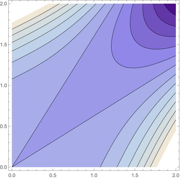
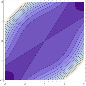
 $d\geq 0$, as visualizedFootnote 7 in figures 1 and 2. Indeed, such negative growth conditions are often employed to simplify the otherwise cumbersome task of showing that a function is not polyconvex [Reference Alibert and Dacorogna1, Reference Ball5, Reference Dacorogna16] (cf. [Reference Aubert3, remark (1)]). Therefore, the examples of rank-one convex functions which are not polyconvex encountered in the literature are usually not suitable to falsify conjecture 1.1.
The sublevels of the energy  $W_{\mathrm {A}}$ on
 $\textrm {GL}^{\!+}(2)$ are connected but not compact.

The sublevels of the extension of  $W_{\mathrm {A}}$ to
 $\mathbb {R}^{2\times 2}$ are neither connected nor compact.

This observation is highlighted further by another important example (which is a homogeneous polynomial expression of grade 4 as well): for the family of isotropic energies
 \begin{equation} W_{\mathrm{ADM}}^{\gamma}\colon\mathbb{R}^{2\times 2}\to\mathbb{R},\qquad W_{\mathrm{ADM}}^{\gamma}(F) = \lVert F \rVert^{2} (\lVert F \rVert^{2}-2\gamma \det F),\qquad \gamma\in\mathbb{R}, \end{equation}
it was shown by Alibert, Dacorogna and Marcellini [Reference Alibert and Dacorogna1, Reference Dacorogna, Marcellini and Ball17] that (cf. figure 3)
 \begin{align*} W_{\mathrm{ADM}}^{\gamma} \quad \text{is convex on } \mathbb{R}^{2\times 2}\quad &\iff \quad \lvert \gamma \rvert\leq \frac{2\sqrt{2}}{3}\approx 0.942809,\\ W_{\mathrm{ADM}}^{\gamma}\quad \text{is polyconvex on } \mathbb{R}^{2\times 2}\quad &\iff \quad\lvert \gamma \rvert\leq 1,\vphantom{\frac 23}\\ W_{\mathrm{ADM}}^{\gamma} \quad \text{is quasiconvex on } \mathbb{R}^{2\times 2}\quad &\iff \quad\lvert \gamma \rvert\leq \gamma_q \ \ \text{with}\ \ \gamma_q>1,\vphantom{\frac 23}\\ W_{\mathrm{ADM}}^{\gamma} \quad \text{is rank-one convex on } \mathbb{R}^{2\times 2}\quad &\iff \quad \lvert \gamma \rvert\leq \frac{2}{\sqrt{3}}\approx 1.1547 \,. \end{align*}
Again, in the nonpolyconvex case  $\lvert \gamma \rvert >1$, the sublevel sets are not compact, since
 $W_{\mathrm {ADM}}(a\cdot \mathbb {1})=4 a^{4}(1-\gamma )<0$ for all
 $a>0$ if
 $\gamma >1$ and
 $W_{\mathrm {ADM}}(\textrm {diag}(a,\,-a))=4 a^{4}(1+\gamma )<0$ for all
 $a>0$ if
 $\gamma <-1$, where
 $\textrm {diag}(x,\,y)\in \mathbb {R}^{2\times 2}$ denotes the diagonal matrix with diagonal entries
 $x,\,y\in \mathbb {R}$.
A schematic overview for the Alibert-Dacorogna-Marcellini family of energies. It is currently unknown whether  $\gamma _q<\frac {2}{\sqrt {3}}$.

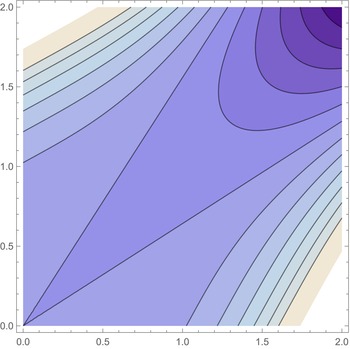
The sublevels of  $W_{\mathrm {ADM}^{+}}^{1.1}$ are connected, but unbounded and thus not compact.

The sublevels of  $W_{\mathrm {ADM}^{+}}^{0.97}$, which are connected and bounded but not compact.

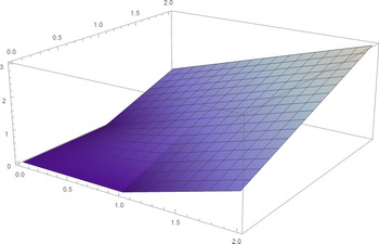
The energy  $W_{\mathrm {S}^{+}}(F)$ on
 $\textrm {GL}^{\!+}(2)$ in terms of singular values of
 $F$.

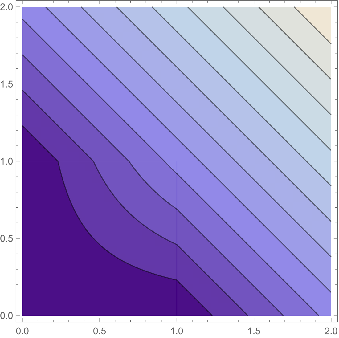
The sublevels of the energy  $W_{\mathrm {S}^{+}}$ on
 $\textrm {GL}^{\!+}(2)$ are connected, but not compact.

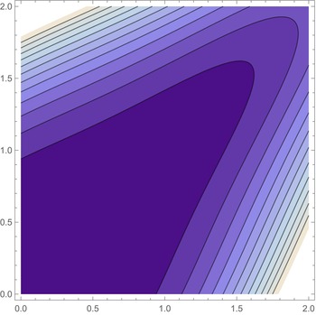
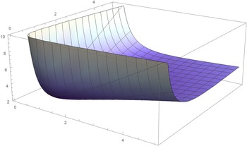
The energy function  $W_0$ in terms of singular values.

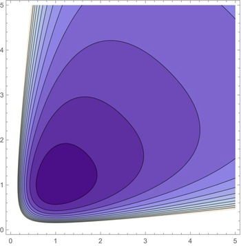
The sublevels of the energy  $W_0$ are compact and connected.

Now, for  $\gamma \in \mathbb {R}$, consider the restriction
 \begin{equation} W_{\mathrm{ADM}^{+}}^{\gamma} = W_{\mathrm{ADM}}^{\gamma}\big|_{\textrm{GL}^{\!+}(2)}\colon\textrm{GL}^{\!+}(2)\to\mathbb{R},\quad W_{\mathrm{ADM}}^{\gamma}(F) = \lVert F \rVert^{2} (\lVert F \rVert^{2}-2\gamma \det F) \end{equation}
of  $W_{\mathrm {ADM}}^{\gamma }$ to
 $\textrm {GL}^{\!+}(2)$. Then
 $W_{\mathrm {ADM}^{+}}^{\gamma }$ can be expressed in terms of (unordered) singular values
 $\lambda _1,\,\lambda _2$ of
 $F\in \textrm {GL}^{\!+}(2)$ via
 \begin{equation} W_{\mathrm{ADM}}^{\gamma}(F)=(\lambda_1^{2}+\lambda_2^{2})^{2}-2 \,\gamma\,(\lambda_1^{2}+\lambda_2^{2}) \,\lambda_1 \lambda_2\,. \end{equation}
In this case, the sublevel sets are not compact for any  $\gamma \in \mathbb {R}$; observe that for every
 $c>0$, since
 \[ \lim_{n\to\infty}\,W_{\mathrm{ADM}^{+}}\Bigl(\frac 1n\cdot\mathbb{1}\Bigr) = \lim_{n\to\infty}\,\frac{4 (1-\gamma)}{n^{4}} = 0, \]
we find  $\frac 1n\cdot \mathbb {1}\in S_c$ for all sufficiently large
 $n\in \mathbb {N}$, thus the sublevel set
 $S_c$ contains a sequence without a subsequence which converges in
 $\textrm {GL}^{\!+}(2)$.
Remark 2.12 From generalizing the above argument, it follows that the compactness of sublevel sets for an energy on  $\textrm {GL}^{\!+}(2)$ requires
 $W$ to satisfy the growth condition
 $W(F)\to \infty$ for
 $\det F\to 0$. In particular, this condition is never satisfied by any polynomial function
 $W$, which immediately excludes the class of polynomial energies as possible counterexamples to conjecture 1.1.
Another example of an  $\textrm {O}(2)$-invariant energy which is rank-one convex but not polyconvex was introduced by Šilhavý [Reference Šilhavý40], who proposed the function
 $W_{\mathrm {S}}\colon \mathbb {R}^{2\times 2}\to \mathbb {R}$ given by
 \begin{align*}
& W_{\mathrm{S}}\colon\mathbb{R}^{2\times 2}\to
\mathbb{R},\quad W_{\mathrm{S}}(F)
={\widehat{g}}_{\mathrm{S}}(\widehat \lambda(F))
\qquad\text{with} \\
& \qquad {\widehat{g}}_{\mathrm{S}}\colon\mathcal{V}_2\to\mathbb{R},\quad
{\widehat{g}}_{\mathrm{S}}(\widehat \lambda_1,\widehat
\lambda_2) =\begin{cases} \widehat \lambda_1\widehat
\lambda_2 & :\widehat \lambda_1\leq 1\\ \widehat
\lambda_1+\widehat \lambda_2 -1 & : \widehat \lambda_1\geq
1\\ \end{cases} \end{align*}
in terms of ordered singular values  $\widehat \lambda _1,\,\widehat \lambda _2$. Again, if we consider the restriction
 $W_{\mathrm {S}^{+}}=W_{\mathrm {S}}|_{\textrm {GL}^{\!+}(2)}$ of
 $W_{\mathrm {S}}$ to
 $\textrm {GL}^{\!+}(2)$, then the sublevel sets (cf. figures 6 and 7) are generally not compact due to the boundedness of
 $W_{\mathrm {S}^{+}}(F)$ for
 $\det F\to 0$.
3. The counterexample
In the following, we will show that the energy function
 \begin{align}
W_0\colon\textrm{GL}^{\!+}(2)\to\mathbb{R},\quad W_0(F)
&= \frac{{\pmb{\boldsymbol{|}}}{F}{\pmb{\boldsymbol{|}}}^{2}}{\det F} -
\log\biggl(\frac{{\pmb{\boldsymbol{|}}}{F}{\pmb{\boldsymbol{|}}}^{2}}{\det
F}\biggr) + \log(\det F) + \frac{1}{\det F}\nonumber\\ &=
\frac{\lambda_{\max}}{\lambda_{\min}} -
\log\left(\frac{\lambda_{\max}}{\lambda_{\min}}\right) +
\log(\lambda_{\max}\lambda_{\min}) +
\frac{1}{\lambda_{\max}\lambda_{\min}}\, \end{align}
is not polyconvex, although it satisfies all the conditions posed in conjecture 1.1, i.e.  $W_0$ is isotropic and rank-one convex with connected, compact sublevel sets; here and in the following, we denote the singular values of
 $X\in \mathbb {R}^{2\times 2}$ by
 $\lambda _{\max }(X)\geq \lambda _{\min }(X)$ and simply write
 $\lambda _{\max },\,\lambda _{\min }$ for the ordered singular values of the energy's argument
 $F$, while
 ${\pmb {\boldsymbol {|}}}{X}{\pmb {\boldsymbol {|}}}=\sup _{\lVert h \rVert =1}\lVert X\, h \rVert =\lambda _{\max }(X)$ denotes the operator norm of any
 $X\in \mathbb {R}^{2\times 2}$.
In order to establish that the desired properties hold for  $W_0$, we will require a number of auxiliary results concerning the sublevel sets of isotropic functions with a so-called volumetric-isochoric split, i.e. functions of the form
 \begin{equation} W\colon\textrm{GL}^{\!+}(2)\to\mathbb{R},\qquad W(F) = W_{\textrm{iso}}(F) + W_{\textrm{vol}}(\det F) \end{equation}
with  $W_{\textrm {iso}}\colon \textrm {GL}^{\!+}(2)\to \mathbb {R}$ and
 $W_{\textrm {vol}}\colon \mathbb {R}_+=(0,\,\infty )\to \mathbb {R}$ such that
 $W_{\textrm {iso}}$ is isochoric, i.e. satisfies
 $W(aF)=W(F)$ for all
 $a>0$. If
 $W_{\textrm {iso}}$, and therefore
 $W$, is objective and isotropic, then any function
 $W$ of the form (3.2) can be expressed as [Reference Martin, Ghiba and Neff25]
 \begin{equation} W(F) = {\widehat{h}}(K(F)) + f(\det F) = \underbrace{{\widehat{h}}\left(\frac{\lambda_{\max}}{\lambda_{\min}}\right)}_{{=}W_{\textrm{iso}}(F)} + \underbrace{f(\lambda_{\max}\lambda_{\min}) \vphantom{\left(\frac{\lambda_{\max}}{\lambda_{\min}}\right)}}_{{=}W_{\textrm{vol}}(\det F)} \end{equation}
for all  $F\in \textrm {GL}^{\!+}(2)$ with singular values
 $\lambda _{\max }\geq \lambda _{\min }>0$ and with uniquely defined functions
 ${\widehat {h}}\colon [1,\,\infty )\to \mathbb {R}$ and
 $f\colon (0,\,\infty )\to \mathbb {R}$. Here,
 \begin{equation}
K\colon\textrm{GL}^{\!+}(2)\to\mathbb{R},\qquad K(F)
\colon=
\frac{{\pmb{\boldsymbol{|}}}{F}{\pmb{\boldsymbol{|}}}^{2}}{\det
F} = \frac{\lambda_{\max}}{\lambda_{\min}}
\end{equation}
is the linear distortion (or dilation) function, which plays an important role in the theory of conformal and quasiconformal mappings [Reference Astala, Iwaniec and Martin2] as well as for the characterization of rank-one convexity, quasiconvexity and polyconvexity of isochoric planar energy functions [Reference Martin, Ghiba and Neff25, Reference Martin, Voss, Ghiba, Sander and Neff27]. More specifically, the isochoric part  $W_{\textrm {iso}}$ of an energy
 $W$ of the form (3.2) is rank-one convex, quasiconvex and polyconvex if and only if the function
 ${\widehat {h}}\colon [1,\,\infty )\to \mathbb {R}$ given by (3.3) is nondecreasing and convex [Reference Martin, Ghiba and Neff25, theorem 3.3]. This equivalence between polyconvexity and rank-one convexity does not hold for the full energy
 $W$ itself, as the example
 $W_0$ will show.
It is clear that  $W_0$ from (3.1) can be expressed in the form (3.2) with
 \begin{equation} W_{\textrm{iso}}(F) = K(F) - \log(K(F)) = \frac{\lambda_{\max}}{\lambda_{\min}} - \log\left(\frac{\lambda_{\max}}{\lambda_{\min}}\right) \end{equation}
and
 \begin{equation} W_{\textrm{vol}}(\det F) = \log(\det F) + \frac{1}{\det F} = \log(\lambda_{\max}\lambda_{\min}) + \frac{1}{\lambda_{\max}\lambda_{\min}} \end{equation}
or, equivalently, in the form (3.3) with
 \begin{equation} {\widehat{h}}(t) = t-\log(t) \qquad\text{and}\qquad f(t)=\frac 1t-\log\left(\frac{1}{t}\right)\,. \end{equation}
As shown in figures 8 and 9, the growth behaviour of  $W_0(F)$ for
 $\det F\to 0$ clearly distinguishes
 $W_0$ from the examples considered in §2.2.
3.1. Auxiliary results for volumetric-isochorically split energy functions
In order to establish  $W_0$ as a counterexample to conjecture 1.1, we first state a sufficient criterion for the compactness of the sublevel sets for energy functions with a volumetric-isochoric split.
Lemma 3.1 Let  $W\colon \textrm {GL}^{\!+}(2)\to \mathbb {R}$ be of the form (3.3) such that
 ${\widehat {h}},\,f$ are lower semicontinuous and
 \begin{equation} \lim_{t\to\infty}{\widehat{h}}(t)=\lim_{t\to\infty}f(t)=\lim_{t\to 0}f(t)=\infty\,. \end{equation}
Then every sublevel set of  $W$ is compact.
Proof. Since all sublevel sets of lower semicontinuous functions are closed (in this case relative to  $\textrm {GL}^{\!+}(2)$), we only need to show that for each
 $c\in \mathbb {R}$, the corresponding sublevel set
 \[ S_c \colon= \{F\in\mathbb{R}^{2\times 2} \,|\, \det F > 0,\; W(F) \leq c\} \]
is bounded and that  $\textrm {dist}(S_c,\,\partial \textrm {GL}^{\!+}(2))>0$. In order to simplify the computations, we will consider the distance on
 $\mathbb {R}^{2\times 2}$ with respect to the operator norm, given by the largest singular value
 $\pmb{\boldsymbol {|}}{X}\pmb{\boldsymbol {|}}=\lambda _{\max }(X)$ of a matrix
 $X\in \mathbb {R}^{2\times 2}$. First note that
 \begin{equation}
{\pmb{\boldsymbol{|}}}{F}\pmb{\boldsymbol {|}}^{2} =
\frac{\lambda_{\max}}{\lambda_{\min}}\cdot\lambda_{\max}\lambda_{\min}
= K(F)\cdot\det(F)
\end{equation}
and that the lower semicontinuity of  ${\widehat {h}}$ and
 $f$, together with (3.8), ensures that both
 ${\widehat {h}}$ and
 $f$ are bounded below by some
 $d\in \mathbb {R}$. Now, let
 $c\in \mathbb {R}$. Then due to (3.8), there exists
 $r\geq 1$ such that
 ${\widehat {h}}(t)>c-d$ and
 $f(t)>c-d$ for any
 $t>r$. Since
 ${\pmb {\boldsymbol {|}}}{F}\pmb{\boldsymbol {|}}^{2}>r^{2}$ implies that either
 $K(F)>r$ or
 $\det (F)>r$ by virtue of (3.9),
 \[ W(F) = {\widehat{h}}(K(F)) + f(\det(F)) > c-d+d = c \]
for any  $F\in \textrm {GL}^{\!+}(2)$ with
 ${\pmb {\boldsymbol {|}}}{F}\pmb{\boldsymbol {|}}>r$. Thus
 $S_c$ is bounded. In order to establish a lower bound for
 $\textrm {dist}(S_c,\,\partial \textrm {GL}^{\!+}(2))$, we first observe that, according to the Eckart-Young-Mirsky Theorem [Reference Mirsky30],Footnote 8
 \begin{align} \textrm{dist}(F,\partial\textrm{GL}^{\!+}(2)) &= \textrm{dist}(F,\{X\in\mathbb{R}^{2\times 2}\,|\,\det(X)=0\}) \nonumber\\ &= \textrm{dist}(F,\{X\in\mathbb{R}^{2\times 2}\,|\,\textrm{rank}(X)\leq 1\}) = \lambda_{\min}(F)\,. \end{align}
Due to (3.8), there exists  $r\leq 1$ such that
 ${\widehat {h}}(s)>c-d$ and
 $f(t)>c-d$ for all
 $t<r$ and all
 $s>\frac 1r$. Then for any
 $F\in \textrm {GL}^{\!+}(2)$ with
 $\lambda _{\min }<r$,
 \[ r^{2} > \lambda_{\min}^{2} = \frac{\lambda_{\max}\lambda_{\min}}{\frac{\lambda_{\max}}{\lambda_{\min}}} = \frac{\det(F)}{K(F)} \]
and thus either  $\det (F)>r$ or
 $K(F)<\frac 1r$. Again,
 $W(F)>c$ in either case; therefore,
 $F\notin S_c$ for any
 $F\in \textrm {GL}^{\!+}(2)$ with
 $\textrm {dist}(F,\,\partial \textrm {GL}^{\!+}(2)) = \lambda _{\min }(F) < r$, which shows that
 $\textrm {dist}(S_c,\,\partial \textrm {GL}^{\!+}(2))\geq r >0$.
We also require a criterion for the sublevel sets of  $W$ to be connected. Recall from definition 2.8 that a function is called q-convex if all its sublevel sets are convex.
Lemma 3.2 Let  $W\colon \textrm {GL}^{\!+}(2)\to \mathbb {R}$ be of the form (3.3) such that
 ${\widehat {h}}\colon [1,\,\infty )\to \mathbb {R}$ is monotone and
 $f$ is q-convex. Then every sublevel set of
 $W$ is connected.
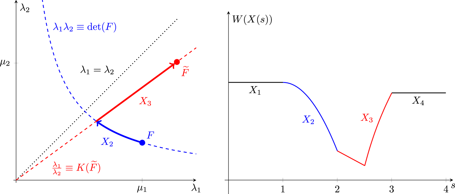
Proof. In order to show that the sublevel set  $S_c$ is (path) connected for any
 $c\in \mathbb {R}$ under the stated conditions, we will explicitly construct a curve connecting arbitrary
 $F,\,{\widetilde {F}}\in S_c$. The construction will be split into four parts, with the first and last one describing a continuous, orthogonal basis change. The second part will be constructed such that the linear distortion
 $K$ is decreasing and the determinant is constant along the curve, while for the third part, the linear distortion
 $K$ is kept constant. This will allow us to utilize the monotonicity of the isochoric part
 ${\widehat {h}}$ and the q-convexity of the volumetric part
 $f$, respectively, to show that the curve remains in the sublevel set (cf. figure 10). For
 $c\in \mathbb {R}$, let
 $F,\,{\widetilde {F}}\in S_c$ and assume without loss of generality that
 $K({\widetilde {F}}) \leq K(F)$. First, choose
 $Q_1,\,Q_2,\,{\widetilde {Q}}_1,\,{\widetilde {Q}}_2\in \textrm {SO}(2)$ such that
 $\textrm {diag}(\lambda _1,\,\lambda _2)\colon= Q_1FQ_2$ and
 $\textrm {diag}(\tilde \lambda _1,\,\tilde \lambda _2)\colon= {\widetilde {Q}}_1{\widetilde {F}}{\widetilde {Q}}_2$ are diagonal with
 $\lambda _1\geq \lambda _2>0$ and
 $\tilde \lambda _1\geq \tilde \lambda _2>0$. Let
 \begin{equation} X_1\colon[0,1]\to\textrm{GL}^{\!+}(2),\qquad X_1(s) = Q_1^{s} FQ_2^{s}\,; \end{equation}
here,  $Q^{s}:= \exp (s\log Q)$ for
 $Q\in \textrm {SO}(2)$, where
 $\log$ denotes the principal matrix logarithm on
 $\textrm {SO}(2)$ or, more explicitly,
 \begin{equation} Q^{s} = \begin{pmatrix} \cos(s \alpha) & \sin(s \alpha)\\-\sin(s \alpha) & \cos(s \alpha) \end{pmatrix} \quad\text{for}\quad Q = \begin{pmatrix} \cos(\alpha) & \sin(\alpha)\\-\sin(\alpha) & \cos(\alpha) \end{pmatrix} \quad\text{with }\;\alpha\in(-\pi,\pi]\,. \end{equation}
In particular,  $X_1$ is continuous with
 $X_1(0)=F$ and
 $X_1(1)=\textrm {diag}(\lambda _1,\,\lambda _2)$. Furthermore,
 $s\mapsto W(X_1(s))$ is constant due to the objectivity and isotropy of
 $W$ and thus, in particular,
 $X_1(s)\in S_c$ for all
 $s\in [0,\,1]$. Now, for
 $\mu _1=\frac {\sqrt {\lambda _1 \lambda _2}}{\sqrt {\tilde \lambda _1 \tilde \lambda _2}}\,\tilde \lambda _1$ and
 $\mu _2=\frac {\sqrt {\lambda _1 \lambda _2}}{\sqrt {\tilde \lambda _1 \tilde \lambda _2}}\,\tilde \lambda _2$, let
 \begin{equation} X_2\colon[0,1]\to\textrm{GL}^{\!+}(2),\qquad X_2(s) = \textrm{diag}(\lambda_1^{1-s} \mu_1^{s},\lambda_2^{1-s} \mu_2^{s})\,. \end{equation}
Then  $X_2$ is continuous with
 $X_2(0)=\textrm {diag}(\lambda _1,\,\lambda _2)=X_1(1)$ and
 $X_2(1)=\textrm {diag}(\mu _1,\,\mu _2)$. Furthermore,
 \begin{align*} \det(X_2(s)) & = \lambda_1^{1-s}
\mu_1^{s} \lambda_2^{1-s} \mu_2^{s} =
\lambda_1\lambda_2\cdot
\biggl(\frac{\mu_1\mu_2}{\lambda_1\lambda_2}\biggr)^{s} \\
& = \lambda_1\lambda_2\cdot \left(\frac{\frac{\sqrt{\lambda_1
\lambda_2}}{\sqrt{\tilde \lambda_1 \tilde
\lambda_2}}\,\tilde \lambda_1\cdot\frac{\sqrt{\lambda_1
\lambda_2}}{\sqrt{\tilde \lambda_1 \tilde
\lambda_2}}\,\tilde
\lambda_2}{\lambda_1\lambda_2}\right)^{s}
= \lambda_1\lambda_2 \end{align*}
is independent of  $s$ and, since
 $\frac {K({\widetilde {F}})}{K(F)}\leq 1$ by assumption, the mapping
 \[ s\mapsto K(X_2(s)) = \frac{\lambda_1^{1-s} \mu_1^{s}}{\lambda_2^{1-s} \mu_2^{s}} = \frac{\lambda_1}{\lambda_2}\cdot \biggl(\frac{\lambda_2 \mu_1}{\lambda_1 \mu_2}\biggr)^{s} = \frac{\lambda_1}{\lambda_2}\cdot \left(\frac{K({\widetilde{F}})}{K(F)}\right)^{s} \]
is nonincreasing on  $[0,\,1]$. Therefore, the assumed monotonicity of the function
 ${\widehat {h}}$ implies that the mapping
 $s\mapsto W(X_2(s))=h(K(X_2(s)))+f(\det (X_2(s)))$ is nonincreasing, hence
 $X_2(s)\in S_c$ for all
 $s\in [0,\,1]$. Next, let
 \[ X_3\colon[0,1]\to\textrm{GL}^{\!+}(2),\qquad X_3(s) = \left(\frac{\sqrt{\tilde \lambda_1 \tilde \lambda_2}}{\sqrt{\lambda_1 \lambda_2}}\right)^{s}\cdot\,\textrm{diag}(\mu_1,\mu_2)\,. \]
Then  $X_3$ is continuous with
 $X_3(0)=\textrm {diag}(\mu _1,\,\mu _2)=X_2(1)$ and
 $X_3(1)=\textrm {diag}(\tilde \lambda _1,\,\tilde \lambda _2)$. We observe that
 $K$ is constant along
 $X_3$ and that
 \[ \min\{\det(X_3(0)), \det(X_3(1))\} \leq\det(X_3(s)) \leq \max\{\det(X_3(0)), \det(X_3(1))\} \]
for all  $s\in [0,\,1]$. Furthermore, the volumetric part
 $f\colon (0,\,\infty )\to \mathbb {R}$ is q-convex by assumption which, in particular [Reference Crouzeix and Ferland15], implies that
 $f(t)\leq \max \{f(a),\,f(b)\}$ for any
 $0<a\leq t \leq b$. We therefore find
 \[ f(\det (X_3(s))) \leq \max\{f(\det(X_3(0) )),\;f(\det(X_3(1)))\} \]
and thus, since  $s\mapsto K(X_3(s))$ is constant (i.e.
 $K(X_3(s))=K(X_3(0))=K(X_3(1))$ for all
 $s\in [0,\,1]$),
 \begin{align*} W(X_3(s)) &= f(\det (X_3(s))) + {\widehat{h}}(K(X_3(s)))\\ &\leq \max\{f(\det(X_3(0))) + {\widehat{h}}(K(X_3(s))),\; f(\det(X_3(1))) + {\widehat{h}}(K(X_3(s)))\}\\ &= \max\{f(\det(X_3(0))) + {\widehat{h}}(K(X_3(0))),\; f(\det(X_3(1))) + {\widehat{h}}(K(X_3(1)))\}\\ &= \max\{W(X_3(0)),\; W(X_3(1))\} \;\leq\; c \end{align*}
for all  $s\in [0,\,1]$. Finally, the curve
 \[ X_4\colon[0,1]\to\textrm{GL}^{\!+}(2),\qquad X_4(s) = ({\widetilde{Q}}_1^{T})^{s} \textrm{diag}(\tilde \lambda_1,\tilde \lambda_2)({\widetilde{Q}}_2^{T})^{s} \]
continuously connects  $\textrm {diag}(\tilde \lambda _1,\,\tilde \lambda _2)$ with
 ${\widetilde {F}}$ such that
 $W$ is constant along
 $X_4$. Therefore, the combined curve
 \[ X\colon[0,4]\to\textrm{GL}^{\!+}(2),\qquad X(s) = X_i(s) \quad\text{ for }\; s\in[i-1,i], \;\;i\in\{1,2,3,4\} \]
is (well defined and) continuous with  $X(0)=F$,
 $X(4)={\widetilde {F}}$ and
 $X(s)\in S_c$ for all
 $s\in [0,\,4]$.
Along  $X_2$, the linear distortion
 $K=\frac {\lambda _1}{\lambda _2}$ is decreasing and the determinant is constant, so the energy is nonincreasing; along
 $X_3$,
 $K$ is constant, so the curve does not leave the sublevel set due to the q-convexity of the energy with respect to the determinant.

Of course, in order to show that  $W_0$ given by (3.1) is a counterexample to conjecture 1.1, the rank-one convexity of
 $W_0$ must be established as well. The following criterion, which is based on an earlier result by Knowles and Sternberg [Reference Knowles and Sternberg23, Reference Knowles and Sternberg24] for twice differentiable functions and which is applicable to volumetric-isochorically split energies in the planar case, has been the subject of a recent contribution [Reference Voss, Ghiba, Martin and Neff44].
Lemma 3.3 [Reference Voss, Ghiba, Martin and Neff44]
For  $f,\,h\in C^{2}((0,\,\infty ))$ with
 $h(\frac 1t)=h(t)$, let
 $W(F)=h\bigl (\frac {\lambda _1}{\lambda _2}\bigr )+f(\lambda _1\lambda _2)$ for all
 $F\in \textrm {GL}^{\!+}(2)$ with singular values
 $\lambda _1,\,\lambda _2$. Then
 $W$ is rank-one convex on
 $\textrm {GL}^{\!+}(2)$ if and only if
(i)
$\displaystyle h_0+f_0\geq 0$,(ii)
$\displaystyle h'(t)\geq 0\qquad \text {for all }\; t\geq 1$,(iii)
$\displaystyle \frac {2t}{t-1} h'(t)-t^{2} h''(t)+f_0\geq 0$ or $\displaystyle a(t)+[b(t)-c(t)]f_0\geq 0\qquad \text {for all } t\in (0,\,\infty ),\,\;t\neq 1$,(iv)
$\displaystyle \frac {2t}{t+1} h'(t)+t^{2} h''(t)-f_0\geq 0\quad \text {or}\quad a(t)+[b(t)+c(t)]f_0\geq 0\qquad \text {for all } t\in (0,\,\infty )$,


where
 \begin{align*} a(t)&=t^{2}(t^{2}-1) h'(t)h''(t)-2t h'(t)^{2},\qquad b(t)=\left(t^{2}+3\right)h'(t)+2t (t^{2}+1) h''(t),\\ c(t)&=4t\left(h'(t)+t h''(t)\right) \end{align*}
and
 \[ h_0=\inf_{t\in(0,\infty)}t^{2} h''(t),\qquad f_0=\inf_{t\in(0,\infty)}t^{2} f''(t)\,.\]
Note that the function  $h\colon (0,\,\infty )\to \mathbb {R}$, which represents the isochoric part of
 $W$ in terms of the ratio
 $\frac {\lambda _1}{\lambda _2}$ of the (not necessarily ordered) singular values, can be obtained from
 ${\widehat {h}}\colon [1,\,\infty )\to \mathbb {R}$ as given in (3.3) by setting
 \begin{equation} h(t) \colon= \begin{cases} {\widehat{h}}(t) & : t\geq 1,\\ {\widehat{h}}\left(\frac 1t\right) & : t<1\,. \end{cases} \end{equation}
Remark 3.4 The energy  $W_0$ can be written in the form
 \[ W_0(F)=h\left(\frac{\lambda_{\max}}{\lambda_{\min}}\right)+h\left(\frac{1}{\lambda_{\max}\lambda_{\min}}\right), \]
where  $h\colon (0,\,\infty )\to \mathbb {R}$ is the function related to
 ${\widehat {h}}\colon [1,\,\infty )\to \mathbb {R}$ with
 ${\widehat {h}}(t)=t-\log (t)$ by (3.14).
3.2. Main properties of the counterexample
We can now prove proposition 1.2, i.e. demonstrate that conjecture 1.1 does not hold, by showing that  $W_0$ is indeed a counterexample.
Proposition 3.5 The function
 \begin{equation} W_0(F) = \frac{\lambda_{\max}}{\lambda_{\min}} - \log\left(\frac{\lambda_{\max}}{\lambda_{\min}}\right) + \log(\lambda_{\max}\lambda_{\min}) + \frac{1}{\lambda_{\max}\lambda_{\min}} = {\widehat{h}}(K(F)) + f(\det F) \end{equation}
with
 \[ {\widehat{h}}(t) = t-\log(t) \qquad\text{and}\qquad f(t)=h\left(\frac{1}{t}\right)=\log(t)+\frac 1t, \]
where  $\lambda _{\max }\geq \lambda _{\min }>0$ are the singular values of
 $F\in \textrm {GL}^{\!+}(2)$, is rank-one convex and isotropic with compact and connected sublevel sets, but not polyconvex.
Proof. The function  $W_0$ is obviously objective and isotropic. Since
 ${\widehat {h}}$ and
 $f$ are lower semicontinuous with
 $\lim _{t\to \infty }{\widehat {h}}(t)=\lim _{t\to \infty }f(t)=\lim _{t\to 0}f(t)=\infty$, lemma 3.1 shows that the sublevel sets of
 $W_0$ are compact. Furthermore,
 ${\widehat {h}}$ is monotone increasing on
 $[1,\,\infty )$ and
 $f$ is q-convex on
 $(0,\,\infty )$, thus the sublevel sets are also connected due to lemma 3.2. It remains to show that
 $W_0$ is rank-one convexFootnote 9 but not polyconvex. In order to prove the rank-one convexity, we will apply lemma 3.3. SinceFootnote 10
 \[ h(t) \;=\; \begin{cases} {\widehat{h}}(t) & : t\geq 1\\ {\widehat{h}}\left(\frac 1t\right) & : t<1 \end{cases} \quad=\quad \begin{cases} t-\log(t) & : t\geq 1\\ \frac 1t+\log(t) & : t<1 \end{cases} \]
for  $t>0$, we find
 \begin{align} h_0 &= \inf_{t\in(0,\infty)}t^{2} h''(t) = \min \left\{ \inf_{t\in[1,\infty)}t^{2} h''(t),\; \inf_{t\in(0,1)}t^{2} h''(t) \right\} \nonumber\\ &= \min \left\{ \inf_{t\in[1,\infty)} t^{2}\cdot\frac{1}{t^{2}},\; \inf_{t\in(0,1)} t^{2}\cdot \left( \frac{2}{t^{3}} -\frac{1}{t^{2}} \right) \right\} = \min \left\{ 1,\; \inf_{t\in(0,1)} \left( \frac{2}{t} -1 \right) \right\} = 1 \end{align}
as well as
 \begin{align*} f_0 &= \inf_{t\in(0,\infty)}t^{2} f''(t) = \inf_{t\in(0,\infty)} t^{2}\cdot \left( -\frac{1}{t^{2}} + \frac{2}{t^{3}} \right) = \inf_{t\in(0,\infty)} -1+\frac{2}{t} ={-}1\,. \end{align*}
Then  $h_0+f_0=0$, thus condition (i) in lemma 3.3 is satisfied. Since
 $h'(t)={\widehat {h}}'(t)=1-\frac 1t\geq 0$ for all
 $t\geq 1$, condition (ii) is fulfilled as well. Next, we compute
 \begin{align*} \frac{2t}{t-1}\,h'(t)-t^{2} h''(t)+f_0 &= \frac{2t}{t-1}\,{\widehat{h}}'(t)-t^{2} {\widehat{h}}''(t)+f_0\\ &= \frac{2t}{t-1}\cdot \left( 1-\frac 1t \right) - t^{2}\cdot \frac{1}{t^{2}} - 1 = \frac{2t}{t-1}\cdot \frac{t-1}{t} - 2 \;=\; 0 \end{align*}
for  $t\geq 1$ as well as
 \begin{align} \frac{2t}{t-1}\,h'(t)-t^{2} h''(t)+f_0 &= \frac{2t}{t-1}\cdot \left( -\frac{1}{t^{2}}+\frac 1t \right) - t^{2}\cdot \left( \frac{2}{t^{3}} - \frac{1}{t^{2}} \right) - 1 \nonumber\\ &= \frac{2t}{t-1}\cdot \frac{t-1}{t^{2}} - t^{2}\cdot \frac{2-t}{t^{3}} - 1 = \frac{2}{t} - \frac{2-t}{t} - 1 \;=\; 0 \end{align}
for  $t<1$, which shows that condition (iii) is also satisfied. Finally, for condition (iv), we find
 \[ \frac{2t}{t+1} h'(t)+t^{2} h''(t)-f_0 = \frac{2t}{t+1}\cdot\frac{t-1}{t} + t^{2}\cdot\frac{1}{t^{2}} + 1 = 2\, \left( \frac{t-1}{t+1}+1 \right) \geq 0 \]
for all  $t\geq 1$ and
 \begin{align*} \frac{2t}{t+1}
h'(t)+t^{2} h''(t)-f_0 &=
\frac{2t}{t+1}\cdot\frac{t-1}{t^{2}} +
t^{2}\cdot\frac{2-t}{t^{3}} + 1\\ &= \frac{2t-2}{t (t+1)} +
\frac{2-t}{t} + 1 = \frac{2t-2}{t (t+1)} + \frac 2t \\
& = \frac{2t-2 + 2 (t+1)}{t (t+1)} = \frac{4}{t+1} \;\geq\; 0
\end{align*}
for all  $t<1$. Therefore, according to lemma 3.3, the function
 $W_0$ is rank-one convex. Finally, in order to show that
 $W_0$ is not polyconvex, we will apply Šilhavý's result given in theorem 2.11. The representation
 ${\widehat {g}}$ of
 $W_0$ in terms of ordered singular values is given by
 \begin{equation} W_0(F) = {\widehat{g}}(\widehat \lambda(F)) \qquad\text{with}\qquad {\widehat{g}}(\widehat \lambda_1,\widehat \lambda_2) = \frac{\widehat \lambda_1}{\widehat \lambda_2} - \log\left(\frac{\widehat \lambda_1}{\widehat \lambda_2}\right) + \log(\widehat \lambda_1\widehat \lambda_2) + \frac{1}{\widehat \lambda_1\widehat \lambda_2}\,. \end{equation}
We compute
 \[ \frac{\partial {\widehat{g}}}{\partial \widehat \lambda_1}=\frac{\widehat \lambda_1^{2}-1}{\widehat \lambda_1^{2} \widehat \lambda_2},\qquad \frac{\partial {\widehat{g}}}{\partial \widehat \lambda_2}={-}\frac{\widehat \lambda_1^{2}-2 \widehat \lambda_1 \widehat \lambda_2+1}{\widehat \lambda_1 \widehat \lambda_2^{2}} \]
and choose
 \[ \gamma_1 = e^{4}, \qquad \gamma_2 = e^{3}, \qquad \nu_1 = e, \qquad \nu_2 = 1\,. \]
Then
 \begin{align}\frac{\partial {\widehat{g}}}{\partial\widehat \lambda_1}(e^{4},e^{3}) &=
\frac{e^{8}-1}{e^{11}}, \qquad \frac{\partial {\widehat{g}}}{\partial\widehat
\lambda_2}(e^{4},e^{3}) = -\frac{e^{7} (e-2)+1}{e^{10}}, \notag \\
-\frac{\frac{\partial {\widehat{g}}}{\partial\widehat
\lambda_1}(e^{4},e^{3})-\frac{\partial {\widehat{g}}}{\partial\widehat
\lambda_2}(e^{4},e^{3})}{e^{4}-e^{3}} &= -\frac{1+e^{8}}{e^{14}}, \notag \\
\frac{\frac{\partial {\widehat{g}}}{\partial\widehat
\lambda_1}(e^{4},e^{3})+
\frac{\partial {\widehat{g}}}{\partial\widehat \lambda_2}(e^{4},e^{3})}{e^{4}+e^{3}}
&= -\frac{1+e-3 e^{8}+e^{9}}{e^{14} (1+e)} \end{align}
and therefore, if  $W_0$ were polyconvex,
 \begin{equation} \begin{aligned} &
\exists\;c\in \left[ -\frac{1+e^{8}}{e^{14}},\;
-\frac{1+e-3 e^{8}+e^{9}}{e^{14} (1+e)} \right] \quad
\text{ such that} \\ & \quad {\widehat{g}}(e,1)\geq
{\widehat{g}}(e^{4},e^{3})+\frac{\partial
{\widehat{g}}}{\partial\widehat
\lambda_1}(e^{4},e^{3})\cdot(e-e^{4}) \\ & \quad +\frac{\partial
{\widehat{g}}}{\partial\widehat
\lambda_2}(e^{4},e^{3})\cdot(1-e^{3})+c\,
(e-e^{4})\,(1-e^{3}) \end{aligned}
\end{equation}
according to theorem 2.11. Since
 \[ {\widehat{g}}(e^{4},e^{3}) = e+6+\frac{1}{e^{7}} \qquad\text{and}\qquad {\widehat{g}}(e,1) = \frac{1}{e}+e, \]
combining (3.20) with (3.19) yields that polyconvexity of  $W_0$ would imply
 \[ \exists\; c\in \left[-\frac{1+e^{8}}{e^{14}},-\frac{1+e-3 e^{8}+e^{9}}{e^{14} (1+e)}\right] \qquad \text{such that}\quad c\leq \frac{2-3 e^{3}-2 e^{7}+e^{9}-4 e^{10}}{e^{11} \left(e^{3}-1\right)^{2}}, \]
in contradiction to
 \[{-}0.00377147 \approx \frac{2-3 e^{3}-2 e^{7}+e^{9}-4 e^{10}}{e^{11} \left(e^{3}-1\right)^{2}}<{-}\frac{1+e^{8}}{e^{14}}\approx{-}0.00247958\,. \]
Therefore, the energy  $W_0$ cannot be polyconvex.
4. Conclusion
We have provided yet another example of a rank-one convex isotropic energy function on  $\textrm {GL}^{\!+}(2)$ which is not polyconvex. In contrast to classical examples encountered in the literature (cf. § 2.2), however, the energy
 $W_0$ given in (3.1) satisfies the growth condition
 $W_0(F)\to \infty$ for
 $\det F \to 0$. Moreover, all sublevel sets of
 $W_0$ are compact as well as connected, thus
 $W_0$ serves as a counterexample to an earlier conjecture by Mielke stating that rank-one convexity of an isotropic function with these properties implies its polyconvexity. As for many other examples of nonpolyconvex planar energy functions, it is currently unknown whether the rank-one convex function
 $W_0$ is quasiconvex as well. In particular, it remains possible that the conditions of conjecture 1.1 are indeed sufficient to ensure the quasiconvexity of rank-one convex planar functions in general.
Acknowledgments
The work of I.D. Ghiba has been supported by a grant of the Romanian Ministry of Research and Innovation, CNCS–UEFISCDI, Project no. PN-III-P1-1.1-TE-2019-0348, Contract No. TE 8/2020, within PNCDI III.
Appendix A. Connectedness of sublevels for Aubert's energy
Although Aubert's example [Reference Aubert3]
 \begin{align*}
W_{\mathrm{A}}\colon\textrm{GL}^{\!+}(2)\to\mathbb{R},\quad
W_{\mathrm{A}}(F) &= \frac 13(\lambda_1^{4}+\lambda_2^{4})
+ \frac 12\lambda_1^{2}\lambda_2^{2} - \frac
23(\lambda_1^{3}\lambda_2+\lambda_1\lambda_2^{3}) \\ & =\frac 13
\lVert F \rVert^{4}-\frac 16 (\det F)^{2}-\frac 23 \det
F\cdot\lVert F \rVert^{2} \end{align*}
of a rank-one convex, nonpolyconvex energy function is not suitable as a counterexample to conjecture 1.1 since the sublevel sets  $S_c$ are not compact, we will show in the following that every set
 $S_c$ is indeed connected.
For  $c\in \mathbb {R}$, let
 $F,\,{\widetilde {F}}\in S_c$. As in the proof of lemma 3.2, we will explicitly construct a continuous curve contained in
 $S_c$ which connects
 $F$ and
 ${\widetilde {F}}$. Without loss of generality,Footnote 11 assume that
 $F=\textrm {diag}(\lambda _1,\,\lambda _2)$ and
 ${\widetilde {F}}=\textrm {diag}(\tilde \lambda _1,\,\tilde \lambda _2)$ are diagonal with
 $\lambda _1\geq \lambda _2$,
 $\tilde \lambda _1\geq \tilde \lambda _2$ and
 $\tilde \lambda _1\geq \lambda _1$. Then the curve
 \begin{equation} X_1\colon[\lambda_2,\lambda_1]\to\textrm{GL}^{\!+}(2),\qquad X_1(s) = \textrm{diag}(\lambda_1,s) \end{equation}
is continuous with  $X_1(\lambda _2)=F$ and, for all
 $s\in [\lambda _2,\,\lambda _1]$,
 \begin{align} \mathrm{d}{s}\;W_{\mathrm{A}}(X_1(s)) &= \frac 43\,s^{3} -
2\lambda_1 s^{2} + \lambda_1^{2}\,s - \frac
23\,\lambda_1^{3} \leq \frac 13\,s^{3} + \lambda_1 s^{2} -
2\lambda_1 s^{2} + \lambda_1^{2}\,s - \frac
23\,\lambda_1^{3}\nonumber\\ &= \frac 13\,s^{3} + \lambda_1
s\,(\lambda_1-s) - \frac 23\,\lambda_1^{3} \leq \frac
13\,s^{3} + \frac 12\,(\lambda_1^{2}+s^{2})\,(\lambda_1-s)
- \frac 23\,\lambda_1^{3} \\ &= \frac 13\,s^{3} + \frac
12\,(\lambda_1^{3}+\lambda_1 s^{2}-\lambda_1^{2} s-s^{3}) -
\frac 23\,\lambda_1^{3} \nonumber \\
& \quad ={-}\frac 16\,s^{3} + \frac
12\,\lambda_1 s\,(s-\lambda_1) - \frac 16\,\lambda_1^{3} \; < \;0\end{align}
where (A.2) holds due to Cauchy's inequality,
 \begin{equation} x\,y\leq k\,x^{2}+\frac{y^{2}}{4\,k} \qquad\text{for all }\; x,y,k>0, \end{equation}
with  $x=\lambda _1$,
 $y=s$ and
 $k=\frac 12$. Therefore, the mapping
 $s\mapsto W_{\mathrm {A}}(X_1(s))$ is monotone decreasing, which implies
 $W_{\mathrm {A}}(X_1(s))\leq W _{\mathrm {A}}(X_1(\lambda _2))=W_{\mathrm {A}}(F)\leq c$ for all
 $s\in [\lambda _2,\,\lambda _1]$.
Now, let
 \[ X_2\colon[\lambda_1,\tilde \lambda_1]\to\textrm{GL}^{\!+}(2),\qquad X_2(s) = \textrm{diag}(s,s)\,. \]
Then  $X_2$ is continuous with
 $X_2(\lambda _1)=X_1(\lambda _1)$. Furthermore,
 $\displaystyle W(X_2(s)) = -\frac {s^{4}}{6},$ thus
 $W_{\mathrm {A}}$ is decreasing along
 $X_2$ as well. Finally, for the continuous curve
 \[ X_3\colon[0,\tilde \lambda_1-\tilde \lambda_2]\to\textrm{GL}^{\!+}(2),\quad X_3(s) = \textrm{diag}(\tilde \lambda_1,\tilde \lambda_1-s), \]
we find  $X_3(0)=X_2(\tilde \lambda _1)$ and
 $X_3(\tilde \lambda _1-\tilde \lambda _2)=\textrm {diag}(\tilde \lambda _1,\,\tilde \lambda _2)={\widetilde {F}}$ as well as
 \begin{align} \mathrm{d}{s}\;W_{\mathrm{A}}(X_3(s)) &= \mathrm{d}{s}\;\left( \frac
13(\tilde \lambda_1^{4}+(\tilde \lambda_1-s)^{4}) + \frac
12\tilde \lambda_1^{2} (\tilde \lambda_1-s)^{2} \right.\nonumber \\
& \quad - \left.\frac 23(\tilde \lambda_1^{3} (\tilde \lambda_1-s)+\tilde
\lambda_1 (\tilde \lambda_1-s)^{3}) \right) \nonumber\\
&= \frac 13\,\tilde \lambda_1^{3} + \tilde \lambda_1^{2}\,s -
2\tilde \lambda_1 s^{2} + \frac 43 s^{3} \geq \frac
13\,\tilde \lambda_1^{3} - \tilde \lambda_1 s^{2} + \frac
43 s^{3} \nonumber\\ &\geq \frac 13\,\tilde \lambda_1^{3} -
s \left( \frac 13 \tilde \lambda^{2} + \frac 34 s^{2}
\right) + \frac 43 s^{3} = \frac 13\,\tilde \lambda^{2}
(\tilde \lambda_1-s) + \left( \frac 43-\frac 34 \right)
s^{3} \;>\; 0, \end{align}
where Cauchy's inequality (A.3) was again employed in (A.4) with  $x=\tilde \lambda _1$,
 $y=s$ and
 $k=\frac 13$. Thus
 $W_{\mathrm {A}}$ is nondecreasing along
 $X_3$, which implies
 \[ W_{\mathrm{A}}(X_3(s)) \leq W_{\mathrm{A}}(X_3(\tilde \lambda_1-\tilde \lambda_2)) = W_{\mathrm{A}}({\widetilde{F}}) \leq c \]
and hence  $X_3(s)\in S_c$ for all
 $s\in [0,\,\tilde \lambda _1-\tilde \lambda _2]$. By concatenating
 $X_1$,
 $X_2$ and
 $X_3$, we therefore obtain a continuous curve contained in
 $S_c$ which connects
 $F$ and
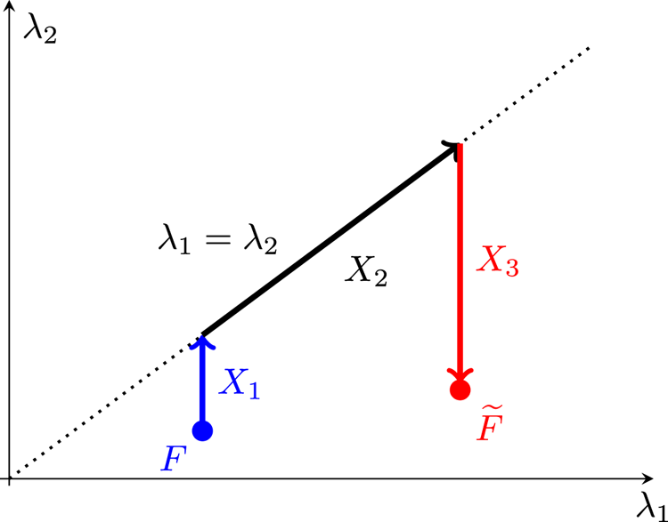
 ${\widetilde {F}}$, cf. figure A1.
The energy  $W_{\mathrm {A}}$ is decreasing along
 $X_1$ and
 $X_2$ and increasing along
 $X_3$.