

Introduction
Biological invasions are considered as a major global threat for ecosystems and for human economics (Mack et al., Reference Mack, Simberloff, Lonsdale, Evans, Clout and Bazzaz2000). A considerable fraction of current biological invasions is a consequence of human activity. Non-native species, for instance, spread as a result of ever-increasing trade and travel, changes in land-use and climate change (Lockwood et al., Reference Lockwood, Hoopes and Marchetti2007). In order to manage and predict invasions, it is essential to understand how environmental variation in time and space affects species’ spread rates. Examining the patterns of spread in historical and still ongoing invasions might provide us with such insights.
Metapopulation or patch occupancy models have been much used to analyse the spatial pattern of biological invasions (Lockwood et al., Reference Lockwood, Hoopes and Marchetti2007). Metapopulation models can account for environmental heterogeneity by letting the exchange rate of individuals between the spatial units (grid cells, habitat patches or hosts) depend on covariates (e.g. Kadoya & Washitani, Reference Kadoya and Washitani2010). Such models can be used to predict in which order patches will become invaded (Eraud et al., Reference Eraud, Boutin, Roux and Faivre2007). If the landscape is assumed to consist of a regular grid of patches, patch occupancy models can be approximated by diffusion–reaction models (which assume local dispersal; Fisher, Reference Fisher1937; Skellam, Reference Skellam1951) or integrodifferential models (which allow for long-distance dispersal; Van den Bosch et al., Reference Van den Bosch, Metz and Diekmann1990; Kot et al., Reference Kot, Lewis and Van den Driessche1996). Both model types express the spread rate with the help of two principal processes: the growth rate of local populations and the displacement of individuals in space (Hastings et al., Reference Hastings, Cuddington, Davies, Dugaw, Elmendorf, Freestone, Harrison, Holland, Lambrinos, Malvadkar, Melbourne, Moore, Taylor and Thomson2005), both of which can be assumed to depend on covariates. Allowing for environmental heterogeneity makes the models mathematically intractable and they need to be solved numerically (Hastings et al., Reference Hastings, Cuddington, Davies, Dugaw, Elmendorf, Freestone, Harrison, Holland, Lambrinos, Malvadkar, Melbourne, Moore, Taylor and Thomson2005). Because of this complication, most of the studies based on diffusion–reaction models have thus assumed homogeneous space, i.e. that the growth of local populations and the displacement of individuals are constant in space and time (though see, e.g. Turchin, Reference Turchin1998). This view has clearly been challenged by empirical studies that have reported high spatial variation in the spread rate (Kuefler et al., Reference Kuefler, Avgar and Fryxell2012), for independent invasions of the same species (Holway, Reference Holway1998), or for different sections of the same invasion front (Evans & Gregoire, Reference Evans and Gregoire2007; Tobin, Reference Tobin2007).
Predictive models of the influence of environmental heterogeneity on the spread rate of invasion are still few (With, Reference With2002; Hastings et al., Reference Hastings, Cuddington, Davies, Dugaw, Elmendorf, Freestone, Harrison, Holland, Lambrinos, Malvadkar, Melbourne, Moore, Taylor and Thomson2005; Lockwood et al., Reference Lockwood, Hoopes and Marchetti2007) compared with the growing amount of data suggesting that such heterogeneity plays an important role. For instance, Cook et al. (Reference Cook, Marion, Butler and Gibson2007) found different rates of colonization in Giant Hogweed Heracleum mantegazzianum for different types of habitats during the invasion in the UK. The invasions of the European Collard Dove in Europe and in the USA are associated with landscape elements related to human settlement such as parks, gardens and high road density (Fujisaki et al., Reference Fujisaki, Pearlstine and Mazzotti2010). Human-mediated transport explains the spread rate of many invertebrates, such as forest pests or water fleas (Daphnia lumholtzi) (Gilbert et al., Reference Gilbert, Gregoire, Freise and Heitland2004). The spread rate of the woody plant species Prunus serotina has been found to increase in areas disturbed by storm and to decrease in areas of active forest management (Sebert-Cuvillier et al., Reference Sebert-Cuvillier, Simon-Goyheneche, Paccaut, Chabrerie, Goubet and Decocq2008). The spread rate of the invasive sugar cane toad in Australia is associated with high temperature, high precipitation, high moisture, availability of water bodies and high density of roads (Urban et al., Reference Urban, Phillips, Skelly and Shine2008). The spread rates of gypsy moth, plant lice and bumblebees are affected by variation in forest composition and winter temperature (Evans & Gregoire, Reference Evans and Gregoire2007; Kadoya & Washitani, Reference Kadoya and Washitani2010).
Although it is evident that habitat suitability for invasive species may change over time (Ficetola et al., Reference Ficetola, Maiorano, Falcucci, Dendoncker, Boitani, Padoa-Schioppa, Miaud and Thuiller2010), most of the studies have described environmental heterogeneity by static maps, thus ignoring the temporal component of environmental variability (Thuiller et al., Reference Thuiller, Richardson, Pysek, Midgley, Hughes and Rouget2005). For instance, climatic and meteorological data are usually implemented as mean or maximum temperature during a certain biologically relevant time frame (Evans & Gregoire, Reference Evans and Gregoire2007), and habitat cover is often assumed to remain static during the invasion history (e.g. Pitt et al., Reference Pitt, Worner and Suarez2009). One major reason why spatiotemporal variability in environmental conditions is seldom accounted for in invasion studies is that the detailed information on the variability of the environment is labour intensive to collect (Lockwood et al., Reference Lockwood, Hoopes and Marchetti2007). Often the invasion is not recognized and properly monitored until it becomes an economical concern and has already spread over a substantial area.
Empirical examples of spatiotemporally varying invasion rates are provided, for instance, by insects that invade new habitats opportunistically when conditions are favourable (Loxdale & Lushai, Reference Loxdale and Lushai1999). Such a spread can lead to alternative invasion trajectories and to jump dispersal, in which satellite populations are found in advance of the main front (Shigesada et al., Reference Shigesada, Kawasaki and Takeda1995). A further complication with understanding and predicting invasion rates is that biotic interactions may exert a dominant role in governing distributional changes, especially at larger spatial scales (Araujo & Luoto, Reference Araujo and Luoto2007). Spatiotemporal variation in host density is recognized as one of the import factors driving epidemics (e.g. Keeling et al., Reference Keeling, Woolhouse, Shaw, Matthews, Chase-Topping, Haydon, Cornell, Kappey, Wilesmith and Grenfell2001).
The example of the deer ked (Lipoptena cervi Hippoboscidae, Linnaeus 1758) invasion in Finland offers the opportunity to investigate if temporal and spatial variations in the environment, more specifically in the host density, has influenced the spread rate. Deer ked is a blood-sucking ectoparasitic louse fly (order of Diptera) of ungulates occurring in the Central Europe and Asia (Haarlov, Reference Haarlov1964). Relatively little is known about the biology of deer ked. At its adult stage the deer ked is permanently attached to its host. Record numbers of 17,000 parasites on a single host have been counted (Paakkonen et al., Reference Paakkonen, Mustonen, Roininen, Niemelä, Ruusila and Nieminen2010). Deer ked is viviparous, each female producing ca. 20–32 pupae during its lifetime. The pupae are dropped off the host, one at a time, over the entire reproductive period of 4–10 months (Haarlov, Reference Haarlov1964). Pupae overwinter on the ground and are able to survive even harsh winter conditions (Härkönen et al., Reference Härkönen, Härkönen, Kaitala, Kaunisto, Kortet, Laaksonen and Ylönen2010, Reference Härkönen, Kaitala, Kaunisto and Repo2012). Juveniles eclose as adults in late autumn of the consecutive year. Newly emerged adults wait passively until a potential host is close by and thereupon fly actively towards the host (Hackman et al., Reference Hackman, Rantanen and Vuojolahti1983). In Finland, the deer ked also often attacks mistakenly humans (Kortet et al., Reference Kortet, Härkönen, Hokkanen, Härkönen, Kaitala, Kaunisto, Laaksonen, Kekäläinen and Ylönen2010), causing allergic reactions and may even propagate diseases such as Bartonella schoenbuchensis (Laukkanen et al., Reference Laukkanen, Ruoppi and Mäkinen-Kiljunen2005; Duodu et al., Reference Duodu, Madslien, Hjelm, Molin, Paziewska-Harris, Harris, Colquhoun and Ytrehus2013). This disturbing behaviour of the deer ked raised the attention of local people soon after the deer ked arrived in Finland, and specimens were sent to the Natural History Museum of Finland already at the early phase of the invasion. These specimens have later helped to reconstruct the invasion history of the ked.
The first observation of deer ked in Finland dates back to 1960 and since then it has made a rapid spread across half of the country (Hackman, Reference Hackman1972; Välimäki et al., Reference Välimaki, Madslien, Malmsten, Härkönen, Härkönen, Kaitala, Kortet, Laaksonen, Mehl, Redford, Ylönen and Ytrehus2010). In Finland, the primary host is Eurasian moose (Alces alces) and thus its density is likely to be an important factor affecting the spread of the ked (Kaitala et al., Reference Kaitala, Kortet, Härkönen, Laaksonen, Härkönen, Kaunisto and Ylönen2009). The Finnish moose populations have undergone great spatiotemporal fluctuations, mainly due to shifts in hunting and forest management (Tiilikainen et al., Reference Tiilikainen, Solberg, Nygrén and Pusenius2012). Overhunting caused the number of moose to decline to such a low level in the 1950s that eventually moose was declared protected in 1969. The complete hunting ban lasted for 2 years (Luoma, Reference Luoma2002), after which hunting started in a regulated manner. The moose population recovered fast in the 1970s (Luoma, Reference Luoma2002) (fig. 1). Currently, the Finnish moose population consists of ca. 89,000–105,000 individuals (Pusenius et al., Reference Pusenius, Tykkyläinen, Wallén, Karhapää, Jouko and Kimmo2009).
Temporal fluctuation of the moose density in Finland during the period of deer ked invasion. The solid line shows the average density over the entire country, and the dotted line shows the 5 and 95% margin of the data among the hunting districts.

This has led to the speculation that the fast increasing density of moose in Finland in the 1970s might have facilitated the deer ked invasion (Von Brander, Reference Von Brander1976; Kaitala et al., Reference Kaitala, Kortet, Härkönen, Laaksonen, Härkönen, Kaunisto and Ylönen2009). As moose is a valuable game species, estimates of moose density are available from different hunting districts for most of the invasion periods of the deer ked. The spread of the deer ked is not systematically documented at a high spatial resolution, but information of the spatial pattern at the invasion front is available (see below).
Our aim is to test if the spread rate of the deer ked varies with local moose density, and specifically the hypothesis that high moose density leads to a high spread rate. If the hypothesis is supported, our more refined aim is to test whether high moose density elevates the spread rate of the deer ked through increased local growth rate, through increased dispersal ability, or a combination of these two factors. To test these hypotheses, we fit to the observed data different versions of diffusion–reaction models, where the diffusion term, the reaction term or both of these terms are allowed us to depend on moose density. These spatiotemporally heterogeneous models are then compared with each other and to a spatiotemporally homogeneous model using the Bayesian information criterion (BIC) to examine which model is best supported by the data.
Methods
Data on the distribution of the deer ked
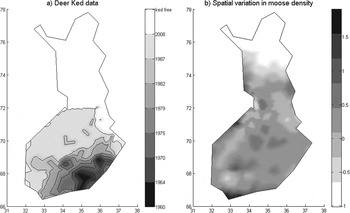
We reconstructed the invasion history of the deer ked in Finland from all seven available publications, which cover the national distribution of the species in the years 1960, 1964, 1970, 1975, 1979, 1981, 1988 and 2008 (Hackman, Reference Hackman1972, Reference Hackman1977, Reference Hackman1979; Von Brander, Reference Von Brander1976; Hackman et al. Reference Hackman, Rantanen and Vuojolahti1983; Zoological Museum Finland, 1988; unpublished data A. Kaitala) (fig. 2a). The quality and the methods of these surveys vary. Data until 1975 consist of specimens and anecdotes reported to the Natural History Museum of Finland; the distribution being described either through individual records or through coarse range outlines (Hackman, Reference Hackman1972, Reference Hackman1977; Von Brander, Reference Von Brander1976). The distributions of 1979 and 2008 are based on records of all locations from which the Natural History Museum of Finland had received specimens up to that date (Hackman, Reference Hackman1979; unpublished data A. Kaitala). In 1981, the data were gathered by a questionnaire that was systematically sent out to forest workers (Hackman et al., Reference Hackman, Rantanen and Vuojolahti1983). In 1988, the data came from the observations of volunteer entomologists through a countrywide survey conducted by the Zoological Museum (Zoological Museum Finland, 1988). Except for the survey in 1981 the survey effort was not systematically controlled for, i.e. there are no data on locations where deer ked has been searched for but not observed. None of the surveys recorded the local density of the deer ked, just the presence of the species. In summary, the data were not systematically collected and there may be a biased distribution of samples, yet the data give a relatively accurate description of the expansion of the main invasion front. Altogether deer ked specimens have been reported in 583 locations.
Illustration of data on deer ked (Lipoptena cervi) and its host moose (Alces alces). a) Shows the range expansion of deer ked over Finland at the spatial resolution of the model, and b) shows an example of spatially varying moose density across Finland in the year 2007, standardized to zero mean and unit variance (moose counts km−2).

We standardized the coordinates of all locations to the Finnish coordinate system YKJ. In cases where the published distribution map did not show any coordinate system, we calculated the coordinates in relation to distinct features of the Finnish national border. To determine the observed spatial distribution of deer ked from surveys recording presence-only data, we used the α-hull technique (Burgman & Fox, Reference Burgman and Fox2003) similarly as in Urban et al. (Reference Urban, Phillips, Skelly and Shine2008). The α-hull is a circumferential line comprising all locations within which deer ked occurred. In contrast to the convex hull, the α-hull does not span edges longer than a threshold value α and thus allows for concavities. We chose α=100 km to reflect the spatial resolution of the data. The resulting α-hulls sometimes comprised two separate hulls, which is biologically plausible, as an isolated observation may represent a distinct satellite population ahead of the main invasion front. According to Hackman et al. (Reference Hackman, Rantanen and Vuojolahti1983) deer ked, in its winged state, is a fairly good flyer but it does usually not fly far from its pupal site and approaches hosts only actively within a distance of ca. 50 m. In contrast, the host moose may move up to 150 km during a year. Deer ked are thus able to hitchhike distances that are several orders of magnitude longer than their flying capacity (Heikkinen, Reference Heikkinen2000).
Data on the moose density
As a tool for hunting management, the size of the moose population has been estimated separately for each hunting district annually since the year 1974, covering all of the 298 hunting districts from 1976 onwards. Hunters estimate the moose density after the autumn hunting period on the basis of observation of tracks in the snow and by sighting of moose throughout the winter. We assumed that the district-based estimate of moose density is valid at the centre of each hunting district, and applied linear interpolation to obtain a continuously varying surface of moose density (fig. 2b). Prior to the year 1974, no systematic district-level counts are available. Nygrén (Reference Nygrén1987) estimated the total number of moose at winter time for the entire country based on various data sources, such as hunting permits, bagged moose, accidents and hunter reports. This is the best available information on moose density for the time between 1960 when the deer ked invasion started and 1974. Since the estimate of Nygrén (Reference Nygrén1987) does not include any information about the spatial distribution of moose density across Finland, we assumed that relative spatial distribution of the density of moose equalled that of the year 1976, which is the first year when moose density was collected for each hunting district.
Model of deer ked invasion
We model the spread of the deer ked following the diffusion–reaction model (Skellam, Reference Skellam1951; Turchin, Reference Turchin1998), which is a partial differential equation modelling both movement (diffusion term) and local growth (reaction term) as
 $$\displaystyle{{{\rm d}u(x,y,t)} \over {{\rm d}t}} = \nabla (D(x,y,t)\nabla u(x,y,t)) + r(x,y,t)u(x,y,t)\left( {1 - \displaystyle{{u(x,y,t)} \over {K(x,y,t)}}} \right)$$
Here u(x, y, t) is the density of deer ked in space (x, y) and time (t), D(x, y, t) is the diffusion coefficient, r(x, y, t) is the population growth rate and K(x, y, t) is the carrying capacity. The derivative with respect to the two-dimensional space is written with the help of the Nabla-operator ∇. The full model in which all of these three parameters may vary arbitrarily is clearly overparameterized to be fitted to our limited data. We thus consider a simpler class of sub-models in which only the parameters D and r are allowed to vary in space and time in a manner that reflects the variation in the density of the host, the moose. As our data contain no information on deer ked abundance, we cannot estimate the carrying capacity K. We thus standardize the equilibrium value of u(x, y, t) to 1 by setting K=1, so that u models the density of deer ked relative to the density that will be reached after the invasion when deer ked can be detected. We parameterized the following set of alternative models in which either (or both) of the diffusion and the reaction terms depend on moose density.
Model 0 (the null-model): D and r are independent of local moose density,
 $$\log (D(x,y,t)) = D_1 $$
 $$r(x,y,t) = r_1 $$
Model 1: D depends on local moose density,
 $$\log (D(x,y,t)) = D_1 + D_2 m(x,y,t)$$
 $$r(x,y,t) = r_1 $$
Model 2: r depends on local moose density,
 $$\log (D(x,y,t)) = D_1 $$
 $$r(x,y,t) = r_1 + r_2 m(x,y,t)$$
Model 3: Both D and r depend on local moose density,
 $$\log (D(x,y,t)) = D_1 + D_2 m(x,y,t)$$
 $$r(x,y,t) = r_1 + r_2 m(x,y,t)$$
Above, m(x, y, t) is the moose density, which we normalized to have zero mean and unit variance overall years and hunting districts. We assumed that the initial condition u(x, y, t 0 )=1 if (x, y) was within the range of the ked in the initial year t 0, and otherwise u(x, y, t 0)=0. We used Matlab as a numerical solver of the diffusion–reaction model; see the appendix for the technical details of the implementation.
Parameter estimation
We initialized the model to correspond to the distribution of the deer ked in the first year t 0=1960 for which the data were available, and solved it with a yearly time step to produce an estimate of deer ked distribution for the next year t=1964 for which empirical data were available. At this point, we compared the predicted density with the observed density (see below), then initialized the model using the observed distribution in t 0=1964, and continued the procedure until the end of the entire study period. We did not have data about the spatial distribution of the deer ked or the density of moose in neighbouring countries, most importantly Russia. We assumed reflecting boundary conditions, and thus made the simplifying assumption that no further net immigration of deer ked occurred from Russia after 1960. This is a conservative assumption because any immigration that may have occurred from Russia will dilute the potential correlation between the spread rate of deer ked and the local moose density. The spread of deer ked occurs parallel to the Finnish–Russian border and thus deer keds moving across the border are less likely to contribute to the advance of the invasion front.
The diffusion–reaction model is a deterministic model describing how population density changes over time. To connect the model prediction to our data, we use the loose interpretation of u(x, y, t) being the probability of the population being present at location x and time t. Then the probability of observing the presence or absence of the species, q(x, y, t)∈0, 1 is
 $$P(\left. q \right|u) = qu + (1 - q)(1 - u)$$
If a number of independent data points would be available at locations (x i , yi ) the total likelihood of the data would be a product of equation 10 over all those locations,
 $$L(q|u) = \prod _i P(q(x_i, y_i, t)|u(x_i, y_i, t))$$
and thus the log-likelihood would be
 $$\log (L(q|u)) = \sum _i \log (P(q(x_i, y_i, t)|u(x_i, y_i, t)))$$
Since our model and distributional data are in continuous space, we consider the limit
 $$\eqalign{ \log (L(\left. q \right|u)) = &\displaystyle{n \over {\left| \Omega \right|}}\int_\Omega {\log (q(x,y,t)u(x,y,t)} \cr & + (1 - q(x,y,t))(1 - u(x,y,t)))\,{\rm d}x\,{\rm d}y} $$
where n denotes the effective number of data points and Ω denotes the total area of Finland. Given the resolution of our raw data and the α-hull technique used to smooth it (fig. 2a), we considered that the effective density of data points was one per 50 km×50 km (Supplementary fig. S1 in the appendix), giving n=135 with |Ω|=338,000 km2.
We applied the Bayesian parameter estimation through an adaptive Metropolis–Hastings MCMC algorithm (Ovaskainen et al., Reference Ovaskainen, Rekola, Meyke and Arjas2008). We assumed log-normal prior distributions for the parameters (D 1, D 2, r 1, r 2) with a mean of μ=−2 and μ=0.01 (for D and r, respectively) and standard deviation of σ=3 for both priors. The technical details of the Metropolis–Hastings algorithm as well as an assessment of the mixing of the MCMC chains are given in the appendix (Supplementary fig. S4 in the appendix).
We compared the four versions of the model with the BIC, which accounts for the fact that a model with a larger number of parameters is more flexible and thus always obtains a higher likelihood even if the added parameter is not of major importance (Schwarz, Reference Schwarz1978). BIC penalizes for the number of model parameters by the formula BIC=−2ln(L)+k(ln(n)), where L is the likelihood, k is the number of model parameters (table 1), and n is the number of data points. We set n=7×135=945 as there were seven surveys against which the model prediction was evaluated, each of which was used to inform the model of the state of the invasion at 135 triangulation grid points (see above).
Model selection – the marginal posterior distributions of model parameters summarized as means and the 95% credible intervals. D 1 is the log-transformed diffusion coefficient at mean moose density, and D 2 is the influence of moose density on diffusion. Similarly, the parameters r 1 and r 2 respectively model the growth rate at mean moose density and the effect of moose density on growth rate. k denotes the number of model parameters, L is the likelihood of the data, and BIC gives the value of the Bayesian information criterion on which model selection was based.

Results
The lowest BIC-value was obtained for the full model 3 in which both the diffusion coefficient and the growth rate were dependent on local moose density (table 1), whereas the spatially homogeneous null model obtained least support. In line with our hypothesis, both the diffusion coefficient and the growth rate increased with local moose density, the 95% credible intervals for the parameters D 2 and r 2 being strictly positive in all models in which they were allowed to vary (table 1). Model 2 performed a little better than model 1, suggesting that moose density operates more strongly through the growth rate than the movement rate.
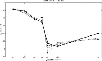
Overall the spatially heterogeneous models fitted the data better than the spatially homogeneous models, but they could not outperform the alternative model in every year. In the survey of 1979 and 1987, the spatially homogeneous random diffusion model (model 0) fitted the data best (fig. 3 and Supplementary figs. S2 and S3 in the appendix). However, the spatially heterogeneous models were able to describe the data in years of a greater dynamic at the deer ked invasion front. Model 3 with growth rate and diffusion coefficient dependent on spatially heterogeneous moose data performed best in the year 1982 and 2008, when the front of the deer ked invasion advanced most. The same trend applied to model 1 and model 2, which performed intermediately for most surveys. Also model 2, with only growth rate dependent on moose, improved its fit in the second half of the invasion period, when the moose density was high (fig. 3).
The contribution of each survey to the log-likelihood of the fitted model 0 (dotted line, open circles), model 1 (broken line, open squares), model 2 (broken line, filled squares) and model 3 (solid line, filled circles). High values of the log-likelihood indicate a better fit of the data to the model.

The estimates of D
1, D
2, r
1 and r
2 of model 3 allow a calculation of the theoretical asymptotic spread rate
 $\sqrt {4Dr} $
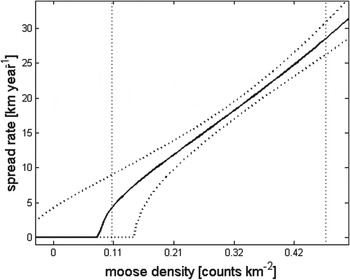
(Skellam, Reference Skellam1951) of the deer ked in homogeneous environment (fig. 4). The mean estimate of average moose density in Finland varied between 0.104 and 0.479 counted moose per km2 during the study period (fig. 1), with mean of 0.296. The mean moose density corresponds to the spread rates of 16.9 km year−1 (posterior mean, with 95% credible interval 15.6–18.2). The lowest observed mean moose density corresponds to the spread rate of 4.0 km year−1 (0.0–9.0), and the highest observed mean moose density to 28.5 km year−1 (26.2–30.1). As the local moose density shows more variation than the mean density over the entire country, the numbers above probably underestimate the range of realized invasion speeds over the study period. The model predicts the threshold density of ca. 0.08 moose per km2 below which the growth rate r becomes negative (fig. 4), suggesting that the spread of deer ked across Finland would have been unlikely for moose densities below this level.
Spread rate of the deer ked invasion predicted by the model 3. The bold solid line shows the posterior median and the dotted lines the 95% credible interval. The vertical dotted lines indicate the lower and the upper range of the annual mean of observed moose densities between 1960 and 2008 (fig. 1).

Discussion
Growing empirical evidence shows that spatiotemporal heterogeneity in environmental conditions can be important for determining the pace of biological invasions. For many parasites and diseases the density of the host is an important determinant of reproduction and dispersal. For example, the spread of the foot and mouth epidemic in France was facilitated by the aggregation of susceptible hosts in time and space (Pioz et al., Reference Pioz, Guis, Crespin, Gay, Calavas, Durand, Abrial and Ducrot2012). Our work suggests that the spread of the deer ked through Finland was influenced by spatiotemporal changes in the density of its main host species, the moose. Our highest ranked model implies that the link between spread rate and host density was due to both the rate of movement (diffusion) and the rate of local growth (reaction) being increased with increasing host density. Adding spatiotemporal changes in the distribution of the host improves model fit, and comparison between the models with respectively r and D dependent on moose densities shows that those including host-dependent growth rates capture observations better than those with only diffusion dependent on local densities. Higher local moose densities mean higher host abundance and allow faster reproduction of deer ked, thus increasing the spread rate.
The highest ranked model predicts a minimal density of 0.08 moose per km2 below which the growth rate becomes negative and the deer ked should not be able to spread. This moose density is slightly below the lowest observed value during the period we modelled. Before 1955, and hence before the invasion started, such low moose densities were the norm in Finland (Luoma, Reference Luoma2002). Our results are thus in line with the hypothesis that the low moose density was the main reason why the invasion of the deer ked in Finland did not start earlier than in 1960 (Von Brander, Reference Von Brander1976; Kaitala et al., Reference Kaitala, Kortet, Härkönen, Laaksonen, Härkönen, Kaunisto and Ylönen2009). Models for deer ked dynamics could be improved with more detailed knowledge about the movement patterns of moose in Finland. In North America, movement of moose occur mainly within local populations and was restricted by roads (Vander Wal et al., Reference Vander Wal, Paquet and Andrés2012). In Norway, moose also migrates between different habitats during the year (Bjorneraas et al., Reference Bjorneraas, Solberg, Herfindal, Van Moorter, Rolandsen, Tremblay, Skarpe, Saether, Eriksen and Astrup2011), which may explain part of the variation in the abundance of deer ked between habitats (Madslien et al., Reference Madslien, Ytrehus, Viljugrein, Solberg, Bråten and Mysterud2012).
An experiment conducted by Härkönen et al. (Reference Härkönen, Härkönen, Kaitala, Kaunisto, Kortet, Laaksonen and Ylönen2010) shows that the deer ked has not yet reached its northern limit in terms of its tolerance to climatic conditions. Further spread north would introduce the deer ked to areas of commercial semi-domestic reindeer husbandry and concerns are that the parasite could cause an economical loss. Reindeer might be an alternative host to deer ked and occur at high densities in these areas (Kynkäänniemi et al., Reference Kynkäänniemi, Kortet, Härkönen, Kaitala, Paakkonen, Mustonen, Nieminen, Härkönen, Ylönen and Laaksonen2010; Välimäki et al., Reference Välimäki, Kaitala, Madslien, Härkönen, Várkonyi, Heikkilä, Jaakola, Ylönen, Kortet and Ytrehus2011). Reindeer forage as large herds with large-scale movements, and this behaviour is likely to increase the potential risk of the spread of the deer ked. However, deer ked reproductive success on reindeer is poorer than on moose and drugs are available to treat reindeer against deer ked (Kynkäänniemi et al., Reference Kynkäänniemi, Kortet, Härkönen, Kaitala, Paakkonen, Mustonen, Nieminen, Härkönen, Ylönen and Laaksonen2010). Large scale treatment or restricting the transport of reindeer could reduce the density of susceptible hosts and thus slower the pace of deer ked invasion or even stop it. The recent halt of the expansion of deer ked indicates that such a strategy could be effective (Välimäki et al., Reference Välimaki, Madslien, Malmsten, Härkönen, Härkönen, Kaitala, Kortet, Laaksonen, Mehl, Redford, Ylönen and Ytrehus2010). More generally, modifying environmental conditions in a way that slows down or stops invasion can be an effective management measure, especially in organisms in which per-capita reproduction rate increases with population density at low density (Tobin et al., Reference Tobin, Berec and Liebhold2011).
Although our model was successful in capturing the overall pattern of spread, it is clearly an oversimplification of reality. Firstly, the model is deterministic, and modelling movements through diffusion implies that displacement distances of all individual are distributed according to the normal distribution (Turchin, Reference Turchin1998). Thus, the model fails to account for the possibility of stochastic long-distance dispersal events. Empirically derived dispersal kernels often have a leptokurtic shape, i.e. a fat tail corresponding to a large number of long-distance dispersal events. Mathematical models that account for a leptokurtic shape of the dispersal kernel predict an increased spread rate (Kot et al., Reference Kot, Lewis and Van den Driessche1996). Stochastic long-distance dispersal events have often found to be of crucial importance for an invasion process (Hastings et al., Reference Hastings, Cuddington, Davies, Dugaw, Elmendorf, Freestone, Harrison, Holland, Lambrinos, Malvadkar, Melbourne, Moore, Taylor and Thomson2005). Stochastic long-distance invasion events have been reported especially due to (often unintentional) human activities (Gilbert et al., Reference Gilbert, Gregoire, Freise and Heitland2004). The large-scale transportation patterns of reindeer might facilitate further spread of the deer ked in the future. However, to estimate for the frequency of such rare events would call for more detailed data than we had available. To mitigate the lack of long-distance dispersal in our model we employed the concept of stratified dispersal (Shigesada et al., Reference Shigesada, Kawasaki and Takeda1995) by continuously updating information on deer ked ranges with available information from surveys, and thus accounted in the initial condition for satellite colonies in advance of the main invasion front.
Secondly, there is growing evidence that invasive species might evolve rapidly, leading to a change in growth rate and redistribution behaviour of the individuals ‘surfing’ the invasion front (Travis & Dytham, Reference Travis and Dytham2002; Phillips et al., Reference Phillips, Brown, Travis and Shine2008; Burton et al., Reference Burton, Phillips and Travis2010). Selection might therefore produce an unsteady spread rate at the invasion front, either through life-history parameters or through host use shifts (Phillips, Reference Phillips2012). Deer ked, for example, might adapt a better cold resistance at the pupae stage, which is the most critical stage during the parasite's life cycle (Härkönen et al., Reference Härkönen, Hurme and Kaitala2013). This would result in an increase local population growth and hence lead to an increased spread rate at higher latitudes. Unfortunately, our data do not allow for testing for evolutionary changes during the spread. In Sweden, a separate population of deer ked is also spreading to the north but at much slower pace than in Finland. Moose density does not explain all of the variation in distributional patterns between the populations, since big uninfected moose populations exist in Sweden well beyond the northern boundary of L. cervi and changes in moose abundance have been more or less parallel across Fennoscandia (Välimäki et al., Reference Välimäki, Kaitala, Madslien, Härkönen, Várkonyi, Heikkilä, Jaakola, Ylönen, Kortet and Ytrehus2011). An explanation for the differential spread rate might be differential use of hosts (in Sweden deer ked commonly uses both moose and roe deer as major hosts), an evolutionary difference or a combination of these two (Välimäki et al., Reference Välimäki, Kaitala, Madslien, Härkönen, Várkonyi, Heikkilä, Jaakola, Ylönen, Kortet and Ytrehus2011).
In conclusion, assessing the links between environmental conditions and invasion processes is critical for gaining understanding on factors influencing invasions and in the development of effective control measures (Liebhold & Tobin, Reference Liebhold and Tobin2008). For many insects, the patterns of spread have been linked with climatic conditions, new colonies being established far from the current distribution during years of favourable conditions (Loxdale & Lushai, Reference Loxdale and Lushai1999; Hochkirch & Damerau, Reference Hochkirch and Damerau2009). In the case of the deer ked, a local peak in moose density can lead to a rapid expansion over an extensive area. Our analysis, based on mapping the dynamics of the invasion front of deer ked to spatiotemporal variation of host density, suggests that the spread rate of the ked varies substantially with host density, with a sevenfold difference between the years of lowest and highest host density in our data (fig. 4).
The appendix can be found in the supplementary material at http://www.journals.cambridge.org/BER
Acknowledgement
We thank Jyrki Pusenius and Tuire Nygrén from the Finnish Game and Fisheries Research Institute for providing us the data and insight on historical moose densities in Finland, and Kimmo Murto for the coordinates of the Finnish hunting districts. This work was supported by the Academy of Finland (C.M.M. 1114864, O.O. 250444); the European Research Council (O.O. ERC Starting Grant 205905); the FWO Research Network ‘Eco-evolutionary dynamics in natural and anthropogenic communities (Eve-Net)’ (D.B. G.0057.09); and FWO projects (C.M.M., D.B. 3G.0610.11).