1 Introduction
Nonlinear effects in oscillatory flow exhibit interesting characteristics, such as streaming that results from oscillatory flows interacting with a solid boundary. Other nonlinear effects can happen with oscillatory disturbances to an otherwise steady flow (Aldridge & Toomre Reference Aldridge and Toomre1969; Busse Reference Busse2010). In this regard the longitudinal librations of rotating planets have generated interest in the spherical geometry (Sauret et al.
Reference Sauret, Cébron, Morize and Le Bars2010; Kida Reference Kida2011; Zhang et al.
Reference Zhang, Chan, Liao and Aurnou2013), including a spherical annulus (Noir et al.
Reference Noir, Hemmerlin, Wicht, Baca and Aurnou2009; Calkins et al.
Reference Calkins, Noir, Eldredge and Aurnou2010; Koch et al.
Reference Koch, Harlander, Egbers and Hollerbach2013; Sauret & Le Dizès Reference Sauret and Le Dizès2013). For purely oscillation-driven flows, streaming involving drops, bubbles and spherical particles have been the subject of many investigations (Riley Reference Riley1966; Amin & Riley Reference Amin and Riley1990; Longuet-Higgins Reference Longuet-Higgins1997, Reference Longuet-Higgins1998; Zhao, Sadhal & Trinh Reference Zhao, Sadhal and Trinh1999a
,Reference Zhao, Sadhal and Trinh
b
; Rednikov, Riley & Sadhal Reference Rednikov, Riley and Sadhal2003; Repetto, Stocchino & Cafferata Reference Repetto, Stocchino and Cafferata2005; Rednikov et al.
Reference Rednikov, Zhao, Sadhal and Trinh2006; Repetto, Siggers & Stocchino Reference Repetto, Siggers and Stocchino2008, Reference Repetto, Siggers and Stocchino2010; Meskauskas, Repetto & Siggers Reference Meskauskas, Repetto and Siggers2011; Rednikov & Sadhal Reference Rednikov and Sadhal2011; Repetto, Siggers & Meskauskas Reference Repetto, Siggers and Meskauskas2014). In terms of torsional motion, Gopinath (Reference Gopinath1994) did some fundamental work on the problem of the exterior region of a sphere. In particular, he considered combined torsional and transverse oscillations of a sphere. Our work focuses on this type of fundamental analysis and concerns where streaming is generated by both transverse and rotational oscillations of the inner sphere. In the present investigation, the two different types of oscillations are combined with the same angular frequency
 $\unicode[STIX]{x1D714}$
. Due to stronger shear stresses resulting from the interaction of two oscillations as compared to a single type of oscillation, such a case is of particular fundamental interest. It should also be noted that with the same angular frequency
 $\unicode[STIX]{x1D714}$
, the effect of the interaction of two oscillations is greatest, and thus, the magnitude of steady streaming induced is strongest, according to Kelly (Reference Kelly1966). In this regard, there is a strong interest in examining the effect of superposed torsional and transverse oscillations in generating the steady streaming with interesting phenomena.
When periodic oscillations are imposed on a body within an incompressible fluid at rest, a steady background appears in addition to the oscillatory flow. This type of non-zero time-averaged flow is referred to as steady streaming. Mathematically, the leading-order solution is oscillatory, and a steady non-zero component exists in the higher-order terms with higher harmonics due to the existence of the nonlinear terms in the Navier–Stokes equation. It was first pointed out by Rayleigh (Reference Rayleigh1884) and later studied by Schlichting (Reference Schlichting1932). Riley (Reference Riley1998, Reference Riley2001) reviewed several examples of acoustic streaming, such as the quartz wind introduced by an ultra-high-frequency beam penetrating a fluid, Rayleigh streaming, and torsional oscillations, as well as free surface flow. More recently, Rednikov & Sadhal (Reference Rednikov and Sadhal2011), Bruus (Reference Bruus2012, Reference Bruus, Laurell and Lenshof2014), Dual et al. (Reference Dual, Hahn, Leibacher, Möller, Schwarz and Wang2012), Sadhal (Reference Sadhal2012a ,Reference Sadhal b ,Reference Sadhal c , Reference Sadhal, Laurell and Lenshof2014), Wiklund (Reference Wiklund2012), Wiklund, Green & Ohlin (Reference Wiklund, Green and Ohlin2012) and Green, Ohlin & Wiklund (Reference Green, Ohlin, Wiklund, Laurell and Lenshof2014) also reviewed several cases of steady streaming. The principles of acoustic streaming have also been presented by Nyborg (Reference Nyborg1953) and Lighthill (Reference Lighthill1978).
Many researchers have studied steady streaming generated by oscillations. The steady streaming introduced by torsional oscillations of a spherical cell containing a fluid drop was examined by Zapryanov & Chervenivanova (Reference Zapryanov and Chervenivanova1981). Three standing vortices in every quadrant between the drop and container, as well as steady streaming inside the drop, were found. In connection with saccadic motion of eyes, Repetto et al. (Reference Repetto, Stocchino and Cafferata2005, Reference Repetto, Siggers and Stocchino2008) studied steady streaming in a spherical chamber undergoing periodic torsional oscillation both theoretically and experimentally, and found good agreement between them. They extended the work by considering the effects of viscoelastic fluids (see Repetto et al. Reference Repetto, Siggers and Meskauskas2014) as well as that of non-spherical geometry (see Stocchino, Repetto & Cafferata Reference Stocchino, Repetto and Cafferata2007; Repetto et al. Reference Repetto, Siggers and Stocchino2010; Bonfiglio et al. Reference Bonfiglio, Repetto, Siggers and Stocchino2013) on steady streaming. The flow generated by small-amplitude torsional oscillation of a sphere in a viscous fluid was presented by Riley (Reference Riley1966), Gopinath (Reference Gopinath1992, Reference Gopinath1993) and Mei (Reference Mei1994). These above-mentioned studies provide descriptions of various cases of steady streaming with torsional and transverse oscillations of a solid sphere and spherical container, corresponding to flows in the regions outside a sphere and within a shell. The steady streaming flow generated by superposed small-amplitude oscillations have been examined by Kelly (Reference Kelly1966), Panagopoulos, Psillakis & Karahalios (Reference Panagopoulos, Psillakis and Karahalios1991) and Riley (Reference Riley1991) for the case of a circular cylinder, and by Gopinath (Reference Gopinath1994) for the case of a sphere. Longuet-Higgins (Reference Longuet-Higgins1998) studied the streaming induced by a spherical bubble undergoing radial and transverse oscillations simultaneously. The streaming phenomenon has been the subject of many recent investigations in connection with manipulation of microparticles with ultrasound (see Jia, Yang & Mei Reference Jia, Yang and Mei2012; Muller et al. Reference Muller, Rossi, Marín, Barnkob, Augustsson, Laurell, Kaehler and Bruus2013). There has also been interest in microstreaming generated by ultrasound on sessile bubbles (see Wang, Rallabandi & Hilgenfeldt Reference Wang, Rallabandi and Hilgenfeldt2013; Rallabandi, Wang & Hilgenfeldt Reference Rallabandi, Wang and Hilgenfeldt2014). Rallabandi et al. (Reference Rallabandi, Wang and Hilgenfeldt2014) considered sessile bubbles attached to a wall with the bubble surface oscillating in multiple modes. In the follow-up work (see Rallabandi et al. Reference Rallabandi, Marin, Rossi, Kähler and Hilgenfeldt2015), three-dimensional flow components resulting from confined geometries were presented. However, little has been considered before about flow induced by superposed oscillations for the fluid between two concentric hemispheres, or spheres for that matter.
In § 2, the theoretical analysis is developed to find solutions to the governing equations. The discussion of results follows in § 3.
2 Model formulation and theoretical development
2.1 Governing equations
There is a viscous fluid between two concentric spheres, the outer one with radius
 $a$
and the inner one
 $R_{i}<a$
. The outer spherical container is held fixed, while the inner sphere is oscillating both torsionally and transversely along the
 $z$
-axis with a phase lag
 $\unicode[STIX]{x1D6FD}^{\prime }$
and with an amplitude difference (with
 $\unicode[STIX]{x1D6FC}$
denoting the amplitude ratio). This problem is three-dimensional axisymmetric, and we formulate it in spherical coordinates.
The dimensional Navier–Stokes and continuity equations are
 $$\begin{eqnarray}\frac{\unicode[STIX]{x2202}\boldsymbol{u}^{\ast }}{\unicode[STIX]{x2202}t^{\ast }}+\boldsymbol{u}^{\ast }\boldsymbol{\cdot }\unicode[STIX]{x1D735}^{\ast }\boldsymbol{u}^{\ast }=-\frac{1}{\unicode[STIX]{x1D70C}}\unicode[STIX]{x1D735}^{\ast }p^{\ast }+\unicode[STIX]{x1D708}{\unicode[STIX]{x1D735}^{\ast }}^{2}\boldsymbol{u}^{\ast },\quad \unicode[STIX]{x1D735}^{\ast }\boldsymbol{\cdot }\boldsymbol{u}^{\ast }=0,\end{eqnarray}$$
with the boundary conditions,
 $$\begin{eqnarray}\displaystyle & \displaystyle u_{r}^{\ast }=U_{0}\sin \unicode[STIX]{x1D714}t^{\ast }\cos \unicode[STIX]{x1D703},\quad u_{\unicode[STIX]{x1D703}}^{\ast }=-U_{0}\sin \unicode[STIX]{x1D714}t^{\ast }\sin \unicode[STIX]{x1D703}, & \displaystyle \nonumber\\ \displaystyle & \displaystyle \text{and}\quad u_{\unicode[STIX]{x1D719}}^{\ast }=\unicode[STIX]{x1D6FC}U_{0}\sin [\unicode[STIX]{x1D714}(t^{\ast }+\unicode[STIX]{x1D6FD}^{\prime })]\sin \unicode[STIX]{x1D703}\quad \text{at }r^{\ast }=R_{i}, & \displaystyle\end{eqnarray}$$
 $$\begin{eqnarray}\displaystyle & \displaystyle u_{r}^{\ast }=u_{\unicode[STIX]{x1D703}}^{\ast }=u_{\unicode[STIX]{x1D719}}^{\ast }=0\quad \text{at }r^{\ast }=a. & \displaystyle\end{eqnarray}$$
 $z$
-axis.
The stream function,
 $\unicode[STIX]{x1D713}^{\ast }$
, and angular circulation,
 $\unicode[STIX]{x1D6FA}^{\ast }$
, related to the velocity components are introduced as
 $$\begin{eqnarray}u_{r}^{\ast }=-\frac{1}{{r^{\ast }}^{2}}\frac{\unicode[STIX]{x2202}\unicode[STIX]{x1D713}^{\ast }}{\unicode[STIX]{x2202}\unicode[STIX]{x1D707}},\quad u_{\unicode[STIX]{x1D703}}^{\ast }=-\frac{(1-\unicode[STIX]{x1D707}^{2})^{-1/2}}{r^{\ast }}\frac{\unicode[STIX]{x2202}\unicode[STIX]{x1D713}^{\ast }}{\unicode[STIX]{x2202}r^{\ast }},\quad u_{\unicode[STIX]{x1D719}}^{\ast }=\frac{\unicode[STIX]{x1D6FA}^{\ast }}{r^{\ast }(1-\unicode[STIX]{x1D707}^{2})^{1/2}},\end{eqnarray}$$
where
 $\unicode[STIX]{x1D707}=\cos \unicode[STIX]{x1D703}$
.
With the velocity, time, radial distance, stream function, angular circulation and shear stress scaled with respect to
 $U_{0}$
,
 $\unicode[STIX]{x1D714}^{-1}$
,
 $a$
,
 $U_{0}a^{2}$
,
 $U_{0}a$
,
 $U_{0}\unicode[STIX]{x1D707}a^{-1}$
we introduce dimensionless variables,
 $$\begin{eqnarray}\boldsymbol{u}=\frac{\boldsymbol{u}^{\ast }}{U_{0}},\quad t=\unicode[STIX]{x1D714}t^{\ast },\quad \unicode[STIX]{x1D713}=\frac{\unicode[STIX]{x1D713}^{\ast }}{U_{0}a^{2}},\quad \unicode[STIX]{x1D6FA}=\frac{\unicode[STIX]{x1D6FA}^{\ast }}{U_{0}a},\quad \unicode[STIX]{x1D735}=a\unicode[STIX]{x1D735}^{\ast },\quad \unicode[STIX]{x1D70F}=\frac{\unicode[STIX]{x1D70F}^{\ast }a}{U_{0}\unicode[STIX]{x1D707}}.\end{eqnarray}$$
The dimensionless governing equations and boundary conditions satisfied by the stream function
 $\unicode[STIX]{x1D713}$
and angular circulation
 $\unicode[STIX]{x1D6FA}$
take the form (Gopinath Reference Gopinath1994),
 $$\begin{eqnarray}\displaystyle & \displaystyle \frac{\unicode[STIX]{x2202}}{\unicode[STIX]{x2202}t}(\text{D}^{2}\unicode[STIX]{x1D713})+\frac{\unicode[STIX]{x1D700}}{r^{2}}\left[\frac{\unicode[STIX]{x2202}(\unicode[STIX]{x1D713},\text{D}^{2}\unicode[STIX]{x1D713})}{\unicode[STIX]{x2202}(r,\unicode[STIX]{x1D707})}+2\text{D}^{2}\unicode[STIX]{x1D713}\text{L}\unicode[STIX]{x1D713}+2\unicode[STIX]{x1D6FA}\text{L}\unicode[STIX]{x1D6FA}\right]=\frac{1}{|M|^{2}}\text{D}^{4}\unicode[STIX]{x1D713}, & \displaystyle\end{eqnarray}$$
 $$\begin{eqnarray}\displaystyle & \displaystyle \frac{\unicode[STIX]{x2202}\unicode[STIX]{x1D6FA}}{\unicode[STIX]{x2202}t}+\frac{\unicode[STIX]{x1D700}}{r^{2}}\left[\frac{\unicode[STIX]{x2202}(\unicode[STIX]{x1D713},\unicode[STIX]{x1D6FA})}{\unicode[STIX]{x2202}(r,\unicode[STIX]{x1D707})}\right]=\frac{1}{|M|^{2}}\text{D}^{2}\unicode[STIX]{x1D6FA}, & \displaystyle\end{eqnarray}$$
 $$\begin{eqnarray}\displaystyle & \displaystyle -\frac{1}{r^{2}}\frac{\unicode[STIX]{x2202}\unicode[STIX]{x1D713}}{\unicode[STIX]{x2202}\unicode[STIX]{x1D707}}=\unicode[STIX]{x1D707}\sin t,\quad -\frac{(1-\unicode[STIX]{x1D707}^{2})^{-1/2}}{r}\frac{\unicode[STIX]{x2202}\unicode[STIX]{x1D713}}{\unicode[STIX]{x2202}r}=-\text{sin}\,t(1-\unicode[STIX]{x1D707}^{2})^{1/2}, & \displaystyle \nonumber\\ \displaystyle & \displaystyle \text{and}\quad \frac{\unicode[STIX]{x1D6FA}}{r(1-\unicode[STIX]{x1D707}^{2})^{1/2}}=\unicode[STIX]{x1D6FC}\sin (t+\unicode[STIX]{x1D6FD})(1-\unicode[STIX]{x1D707}^{2})^{1/2}\quad \text{on }r=b, & \displaystyle\end{eqnarray}$$
 $$\begin{eqnarray}\displaystyle & \displaystyle \unicode[STIX]{x1D713}=\frac{\unicode[STIX]{x2202}\unicode[STIX]{x1D713}}{\unicode[STIX]{x2202}r}=0,\quad \unicode[STIX]{x1D6FA}=0\quad \text{on }r=1, & \displaystyle\end{eqnarray}$$
 $$\begin{eqnarray}\displaystyle & \displaystyle \unicode[STIX]{x1D707}=\cos \unicode[STIX]{x1D703},\quad \unicode[STIX]{x1D6FD}=\unicode[STIX]{x1D714}\unicode[STIX]{x1D6FD}^{\prime },\quad \unicode[STIX]{x1D700}=\frac{U_{0}}{\unicode[STIX]{x1D714}a},\quad |M|^{2}=\frac{\unicode[STIX]{x1D714}a^{2}}{\unicode[STIX]{x1D708}},\quad b=\frac{R_{i}}{a} & \displaystyle \nonumber\\ \displaystyle & \displaystyle \text{D}^{2}=\frac{\unicode[STIX]{x2202}^{2}}{\unicode[STIX]{x2202}r^{2}}+\frac{1-\unicode[STIX]{x1D707}^{2}}{r^{2}}\frac{\unicode[STIX]{x2202}^{2}}{\unicode[STIX]{x2202}\unicode[STIX]{x1D707}^{2}},\quad \text{and}\quad \text{L}=\frac{\unicode[STIX]{x1D707}}{1-\unicode[STIX]{x1D707}^{2}}\frac{\unicode[STIX]{x2202}}{\unicode[STIX]{x2202}r}+\frac{1}{r}\frac{\unicode[STIX]{x2202}}{\unicode[STIX]{x2202}\unicode[STIX]{x1D707}}. & \displaystyle\end{eqnarray}$$
2.2 The leading-order solutions
We start out with the following perturbation expansion,
 $$\begin{eqnarray}\unicode[STIX]{x1D713}=\unicode[STIX]{x1D713}_{0}+\text{H.O.T.},\quad \unicode[STIX]{x1D6FA}=\unicode[STIX]{x1D6FA}_{0}+\text{H.O.T.},\end{eqnarray}$$
where H.O.T. means higher-order terms. Upon substitution into the momentum equation (2.5), the leading-order solutions emerge as
 $$\begin{eqnarray}\displaystyle & \displaystyle \frac{\unicode[STIX]{x2202}}{\unicode[STIX]{x2202}t}(\text{D}^{2}\unicode[STIX]{x1D713}_{0})=\frac{1}{|M|^{2}}\text{D}^{4}\unicode[STIX]{x1D713}_{0}, & \displaystyle\end{eqnarray}$$
 $$\begin{eqnarray}\displaystyle & \displaystyle \frac{\unicode[STIX]{x2202}\unicode[STIX]{x1D6FA}_{0}}{\unicode[STIX]{x2202}t}=\frac{1}{|M|^{2}}\text{D}^{2}\unicode[STIX]{x1D6FA}_{0}. & \displaystyle\end{eqnarray}$$
 $$\begin{eqnarray}\displaystyle \unicode[STIX]{x1D713}_{0} & = & \displaystyle \left[A_{0}r^{2}+\frac{B_{0}}{r}+C_{0}\left(\frac{1}{Mr}-1\right)\text{e}^{Mr}+D_{0}\left(\frac{1}{Mr}+1\right)\text{e}^{-Mr}\right](1-\unicode[STIX]{x1D707}^{2})\text{e}^{\text{i}t}+\text{c.c.}\nonumber\\ \displaystyle & = & \displaystyle f(r)\text{e}^{\text{i}t}(1-\unicode[STIX]{x1D707}^{2})+\text{c.c.},\end{eqnarray}$$
 $$\begin{eqnarray}\displaystyle \unicode[STIX]{x1D6FA}_{0} & = & \displaystyle \left[A_{0}^{\ast }\left(\frac{1}{Mr}-1\right)\text{e}^{Mr}+B_{0}^{\ast }\left(\frac{1}{Mr}+1\right)\text{e}^{-Mr}\right](1-\unicode[STIX]{x1D707}^{2})\text{e}^{\text{i}t}+\text{c.c.}\nonumber\\ \displaystyle & = & \displaystyle g(r)\text{e}^{\text{i}t}(1-\unicode[STIX]{x1D707}^{2})+\text{c.c.},\end{eqnarray}$$
 $$\begin{eqnarray}\displaystyle M^{2}=\text{i}|M|^{2}, & & \displaystyle\end{eqnarray}$$
c.c. denotes the complex conjugate, and details of all the coefficients in (2.10) are provided in appendix B.
The dimensionless shear stresses are
 $$\begin{eqnarray}\displaystyle \unicode[STIX]{x1D70F}_{0r\unicode[STIX]{x1D703}} & = & \displaystyle \left[-\frac{6B_{0}}{r^{4}}+C_{0}\left(-\frac{6}{Mr^{4}}+\frac{6}{r^{3}}-\frac{3M}{r^{2}}+\frac{M^{2}}{r}\right)\text{e}^{Mr}+D_{0}\left(-\frac{6}{Mr^{4}}-\frac{6}{r^{3}}\right.\right.\nonumber\\ \displaystyle & & \displaystyle \left.\left.-\,\frac{3M}{r^{2}}-\frac{M^{2}}{r}\right)\text{e}^{-Mr}\right](1-\unicode[STIX]{x1D707}^{2})^{1/2}\text{e}^{\text{i}t}+\text{c.c.},\end{eqnarray}$$
 $$\begin{eqnarray}\displaystyle \unicode[STIX]{x1D70F}_{0r\unicode[STIX]{x1D719}} & = & \displaystyle \left[A_{0}^{\ast }\left(-\frac{3}{Mr^{3}}+\frac{3}{r^{2}}-\frac{M}{r}\right)\text{e}^{Mr}+B_{0}^{\ast }\left(-\frac{3}{Mr^{3}}-\frac{3}{r^{2}}-\frac{M}{r}\right)\text{e}^{-Mr}\right]\nonumber\\ \displaystyle & & \displaystyle \times \,(1-\unicode[STIX]{x1D707}^{2})^{1/2}\text{e}^{\text{i}t}+\text{c.c.},\end{eqnarray}$$
 $$\begin{eqnarray}\displaystyle \unicode[STIX]{x1D70F}_{0\unicode[STIX]{x1D719}\unicode[STIX]{x1D703}} & = & \displaystyle 0.\end{eqnarray}$$
2.3 The solutions to order
 $\unicode[STIX]{x1D700}$

The variables to order
 $\unicode[STIX]{x1D700}$
are divided into time-independent and time-dependent parts as
 $$\begin{eqnarray}\displaystyle & & \displaystyle \displaystyle \unicode[STIX]{x1D713}_{1}=\unicode[STIX]{x1D713}_{1}^{(s)}+\unicode[STIX]{x1D713}_{1}^{(u)}=\unicode[STIX]{x1D713}_{10}(r,\unicode[STIX]{x1D707})+\{\unicode[STIX]{x1D713}_{12}(r,\unicode[STIX]{x1D707})\text{e}^{2\text{i}t}+\text{c.c.}\},\end{eqnarray}$$
 $$\begin{eqnarray}\displaystyle & & \displaystyle \displaystyle \unicode[STIX]{x1D6FA}_{1}=\unicode[STIX]{x1D6FA}_{1}^{(s)}+\unicode[STIX]{x1D6FA}_{1}^{(u)}=\unicode[STIX]{x1D6FA}_{10}(r,\unicode[STIX]{x1D707})+\{\unicode[STIX]{x1D6FA}_{12}(r,\unicode[STIX]{x1D707})\text{e}^{2\text{i}t}+\text{c.c.}\},\end{eqnarray}$$
 $$\begin{eqnarray}\displaystyle & & \displaystyle \displaystyle \frac{1}{r^{2}}\left[\frac{\unicode[STIX]{x2202}(\unicode[STIX]{x1D713}_{0},\text{D}^{2}\unicode[STIX]{x1D713}_{0})}{\unicode[STIX]{x2202}(r,\unicode[STIX]{x1D707})}+2\text{D}^{2}\unicode[STIX]{x1D713}_{0}\text{L}\unicode[STIX]{x1D713}_{0}+2\unicode[STIX]{x1D6FA}_{0}\text{L}\unicode[STIX]{x1D6FA}_{0}\right]={\mathcal{F}}_{0}+\{{\mathcal{F}}_{2}\text{e}^{2\text{i}t}+\text{c.c.}\},\end{eqnarray}$$
 $$\begin{eqnarray}\displaystyle & & \displaystyle \displaystyle \frac{1}{r^{2}}\left[\frac{\unicode[STIX]{x2202}(\unicode[STIX]{x1D713}_{0},\unicode[STIX]{x1D6FA}_{0})}{\unicode[STIX]{x2202}(r,\unicode[STIX]{x1D707})}\right]={\mathcal{G}}_{0}+\{{\mathcal{G}}_{2}\text{e}^{2\text{i}t}+\text{c.c.}\},\end{eqnarray}$$
 $(s)$
and
 $(u)$
refer to steady and unsteady parts, respectively.
The steady part of the first-order solutions satisfies
 $$\begin{eqnarray}\text{D}^{4}\unicode[STIX]{x1D713}_{10}=|M|^{2}{\mathcal{F}}_{0},\quad \text{D}^{2}\unicode[STIX]{x1D6FA}_{10}=|M|^{2}{\mathcal{G}}_{0},\end{eqnarray}$$
with homogeneous boundary conditions
 $$\begin{eqnarray}\unicode[STIX]{x1D713}_{10}=\frac{\unicode[STIX]{x2202}\unicode[STIX]{x1D713}_{10}}{\unicode[STIX]{x2202}r}=\unicode[STIX]{x1D6FA}_{10}=0\quad \text{on }r=b,\quad \text{and}\quad \unicode[STIX]{x1D713}_{10}=\frac{\unicode[STIX]{x2202}\unicode[STIX]{x1D713}_{10}}{\unicode[STIX]{x2202}r}=\unicode[STIX]{x1D6FA}_{10}=0\quad \text{on }r=1.\end{eqnarray}$$
The steady part of nonlinear terms may be written as
 $$\begin{eqnarray}{\mathcal{F}}_{0}={\mathcal{F}}_{0r}(r)\unicode[STIX]{x1D707}(1-\unicode[STIX]{x1D707}^{2}),\quad {\mathcal{G}}_{0}={\mathcal{G}}_{0r}(r)\unicode[STIX]{x1D707}(1-\unicode[STIX]{x1D707}^{2}),\end{eqnarray}$$
where
 $$\begin{eqnarray}\displaystyle {\mathcal{F}}_{0r}(r) & = & \displaystyle \frac{2}{r^{2}}[f(r)\overline{f^{(3)}(r)}+\overline{f(r)}f^{(3)}(r)+g(r)\overline{g^{^{\prime }}(r)}+\overline{g(r)}g^{\prime }(r)]-\frac{4}{r^{3}} [\!f(r)\overline{f^{^{\prime \prime }}(r)}\nonumber\\ \displaystyle & & \displaystyle +\,\overline{f(r)}f^{\prime \prime }(r)+2g(r)\overline{g(r)}\!]-\frac{4}{r^{4}}[f(r)\overline{f^{^{\prime }}(r)}+\overline{f(r)}f^{\prime }(r)]+\frac{32}{r^{5}}f(r)\overline{f(r)},\nonumber\\ \displaystyle & & \displaystyle\end{eqnarray}$$
 $$\begin{eqnarray}\displaystyle {\mathcal{G}}_{0r}(r) & = & \displaystyle \frac{2}{r^{2}}[f(r)\overline{g^{^{\prime }}(r)}+\overline{f(r)}g^{\prime }(r)-f^{\prime }(r)\overline{g(r)}-\overline{f^{^{\prime }}(r)}g(r)].\end{eqnarray}$$
Next, we express the stream function and angular circulation of steady streaming in forms as
 $$\begin{eqnarray}\unicode[STIX]{x1D713}_{10}=f_{10}(r)\unicode[STIX]{x1D707}(1-\unicode[STIX]{x1D707}^{2}),\quad \unicode[STIX]{x1D6FA}_{10}=g_{10}(r)\unicode[STIX]{x1D707}(1-\unicode[STIX]{x1D707}^{2}).\end{eqnarray}$$
The resulting differential equations to order
 $\unicode[STIX]{x1D700}$
become
 $$\begin{eqnarray}\displaystyle \frac{\text{d}^{4}}{\text{d}r^{4}}f_{10}(r)-\frac{12}{r^{2}}\frac{\text{d}^{2}}{\text{d}r^{2}}f_{10}(r)+\frac{24}{r^{3}}\frac{\text{d}}{\text{d}r}f_{10}(r) & = & \displaystyle |M|^{2}{\mathcal{F}}_{0r}(r),\end{eqnarray}$$
 $$\begin{eqnarray}\displaystyle \frac{\text{d}^{2}}{\text{d}r^{2}}g_{10}(r)-\frac{6}{r^{2}}g_{10}(r) & = & \displaystyle |M|^{2}{\mathcal{G}}_{0r}(r),\end{eqnarray}$$
With the solutions obtained, the velocity can now be expressed as
 $$\begin{eqnarray}\displaystyle u_{10r} & = & \displaystyle \left[c_{1}r^{3}+c_{2}r+\frac{c_{3}}{r^{2}}+\frac{c_{4}}{r^{4}}+H_{1}(r)r^{3}+H_{2}(r)r+\frac{H_{3}(r)}{r^{2}}+\frac{H_{4}(r)}{r^{4}}\right](3\unicode[STIX]{x1D707}^{2}-1),\nonumber\\ \displaystyle & & \displaystyle\end{eqnarray}$$
 $$\begin{eqnarray}\displaystyle u_{10\unicode[STIX]{x1D703}} & = & \displaystyle \left[-5c_{1}r^{3}-3c_{2}r+\frac{2c_{4}}{r^{4}}-5H_{1}(r)r^{3}-3H_{2}(r)r+\frac{2H_{4}(r)}{r^{4}}\right]\unicode[STIX]{x1D707}(1-\unicode[STIX]{x1D707}^{2})^{1/2},\nonumber\\ \displaystyle & & \displaystyle\end{eqnarray}$$
 $$\begin{eqnarray}\displaystyle u_{10\unicode[STIX]{x1D719}} & = & \displaystyle \left[c_{5}r^{2}+\frac{c_{6}}{r^{3}}+H_{5}(r)r^{2}+\frac{H_{6}(r)}{r^{3}}\right]\unicode[STIX]{x1D707}(1-\unicode[STIX]{x1D707}^{2})^{1/2}.\end{eqnarray}$$
The stream function and angular circulation take the form
 $$\begin{eqnarray}\displaystyle \unicode[STIX]{x1D713}_{10} & = & \displaystyle \left[c_{1}r^{5}+c_{2}r^{3}+c_{3}+\frac{c_{4}}{r^{2}}+H_{1}(r)r^{5}+H_{2}(r)r^{3}+H_{3}(r)+\frac{H_{4}(r)}{r^{2}}\right]\unicode[STIX]{x1D707}(1-\unicode[STIX]{x1D707}^{2}),\nonumber\\ \displaystyle & & \displaystyle\end{eqnarray}$$
 $$\begin{eqnarray}\displaystyle \unicode[STIX]{x1D6FA}_{10} & = & \displaystyle \left[c_{5}r^{3}+\frac{c_{6}}{r^{2}}+H_{5}(r)r^{3}+\frac{H_{6}(r)}{r^{2}}\right],\end{eqnarray}$$
 $$\begin{eqnarray}\displaystyle H_{1}(r) & = & \displaystyle -\frac{|M|^{2}}{200}\int _{b}^{r}\frac{{\mathcal{F}}_{0r}(r^{\prime })}{{r^{\prime }}^{2}}\,\text{d}r^{\prime },\end{eqnarray}$$
 $$\begin{eqnarray}\displaystyle H_{2}(r) & = & \displaystyle \frac{7|M|^{2}}{600}\int _{b}^{r}{\mathcal{F}}_{0r}(r^{\prime })\,\text{d}r^{\prime },\end{eqnarray}$$
 $$\begin{eqnarray}\displaystyle H_{3}(r) & = & \displaystyle -\frac{7|M|^{2}}{600}\int _{b}^{r}{\mathcal{F}}_{0r}(r^{\prime }){r^{\prime }}^{3}\,\text{d}r^{\prime },\end{eqnarray}$$
 $$\begin{eqnarray}\displaystyle H_{4}(r) & = & \displaystyle \frac{|M|^{2}}{200}\int _{b}^{r}{\mathcal{F}}_{0r}(r^{\prime }){r^{\prime }}^{5}\,\text{d}r^{\prime },\end{eqnarray}$$
 $$\begin{eqnarray}\displaystyle H_{5}(r) & = & \displaystyle \frac{|M|^{2}}{5}\int _{b}^{r}\frac{{\mathcal{G}}_{0r}(r^{\prime })}{{r^{\prime }}^{2}}\,\text{d}r^{\prime },\end{eqnarray}$$
 $$\begin{eqnarray}\displaystyle H_{6}(r) & = & \displaystyle -\frac{|M|^{2}}{5}\int _{b}^{r}{\mathcal{G}}_{0r}(r^{\prime }){r^{\prime }}^{3}\,\text{d}r^{\prime },\end{eqnarray}$$
While these results are for unrestricted
 $|M|$
, they are mathematically complex. A better insight is achieved with some asymptotic analysis. Therefore, the problem is also discussed separately in the low-frequency
 $(|M|^{2}\ll 1)$
and the high-frequency
 $(|M|^{2}\gg 1)$
limits.
2.4 The low-frequency limit,
$\unicode[STIX]{x1D700}\ll 1\ll |M|^{-2}$

For low frequency, the viscous diffusion thickness is larger than the characteristic dimension of the body, which means vorticity diffuses over a much wider region.
We now seek a perturbation solution of the governing equations in the form
 $$\begin{eqnarray}\displaystyle \unicode[STIX]{x1D713} & = & \displaystyle \unicode[STIX]{x1D713}_{0}+R\unicode[STIX]{x1D713}_{1}+R^{2}\unicode[STIX]{x1D713}_{2}+O(R^{3}),\end{eqnarray}$$
 $$\begin{eqnarray}\displaystyle \unicode[STIX]{x1D6FA} & = & \displaystyle \unicode[STIX]{x1D6FA}_{0}+R\unicode[STIX]{x1D6FA}_{1}+R^{2}\unicode[STIX]{x1D6FA}_{2}+O(R^{3}),\end{eqnarray}$$
 $R$
is the oscillatory Reynolds number, defined as
 $$\begin{eqnarray}R=\unicode[STIX]{x1D700}|M|^{2}=\frac{U_{0}a}{\unicode[STIX]{x1D708}}\ll 1.\end{eqnarray}$$
Then, in the limit of
 $|M|\rightarrow 0$
, equations (2.10) and (2.12) can be simplified to
 $$\begin{eqnarray}\displaystyle \unicode[STIX]{x1D713}_{0} & = & \displaystyle \frac{3b}{2\text{i}(1-b)^{4}(4+7b+4b^{2})}\left[-\frac{1}{3}b^{2}(1-b^{3})\frac{1}{r}+(1-b^{5})r-\frac{1}{6}(9-5b^{2}-4b^{5})r^{2}\right.\nonumber\\ \displaystyle & & \displaystyle \left.+\,\frac{1}{2}(1-b^{2})r^{4}\right](1-\unicode[STIX]{x1D707}^{2})\text{e}^{\text{i}t}+\text{c.c.},\end{eqnarray}$$
 $$\begin{eqnarray}\displaystyle \unicode[STIX]{x1D6FA}_{0} & = & \displaystyle \frac{1}{2\text{i}}\unicode[STIX]{x1D6FC}\text{e}^{\text{i}\unicode[STIX]{x1D6FD}}\frac{b^{2}}{1-b^{3}}\left(\frac{1}{r}-r^{2}\right)(1-\unicode[STIX]{x1D707}^{2})\text{e}^{\text{i}t}+\text{c.c.},\end{eqnarray}$$
 $$\begin{eqnarray}\displaystyle \unicode[STIX]{x1D70F}_{0r\unicode[STIX]{x1D703}} & = & \displaystyle \frac{3b}{2\text{i}(1-b)^{4}(4+7b+4b^{2})}\left[2b^{2}(1-b^{3})\frac{1}{r^{4}}-3(1-b^{2})r\right](1-\unicode[STIX]{x1D707}^{2})^{1/2}\text{e}^{\text{i}t}+\text{c.c.},\nonumber\\ \displaystyle & & \displaystyle\end{eqnarray}$$
 $$\begin{eqnarray}\displaystyle \unicode[STIX]{x1D70F}_{0r\unicode[STIX]{x1D719}} & = & \displaystyle -\left(\frac{3\unicode[STIX]{x1D6FC}\text{e}^{\text{i}\unicode[STIX]{x1D6FD}}}{2\text{i}}\right)\left(\frac{b^{2}}{1-b^{3}}\right)\frac{1}{r^{3}}(1-\unicode[STIX]{x1D707}^{2})^{1/2}\text{e}^{\text{i}t}+\text{c.c.},\end{eqnarray}$$
 $$\begin{eqnarray}\displaystyle \unicode[STIX]{x1D70F}_{0\unicode[STIX]{x1D719}\unicode[STIX]{x1D703}} & = & \displaystyle 0.\end{eqnarray}$$
Next, solutions of
 $O(R)$
satisfy
 $$\begin{eqnarray}\displaystyle \text{D}^{4}\unicode[STIX]{x1D713}_{1} & = & \displaystyle \frac{1}{r^{2}}\left[\frac{\unicode[STIX]{x2202}(\unicode[STIX]{x1D713}_{0},\text{D}^{2}\unicode[STIX]{x1D713}_{0})}{\unicode[STIX]{x2202}(r,\unicode[STIX]{x1D707})}+2\text{D}^{2}\unicode[STIX]{x1D713}_{0}\text{L}\unicode[STIX]{x1D713}_{0}+2\unicode[STIX]{x1D6FA}_{0}\text{L}\unicode[STIX]{x1D6FA}_{0}\right]+O(|M|),\end{eqnarray}$$
 $$\begin{eqnarray}\displaystyle \text{D}^{4}\unicode[STIX]{x1D6FA}_{1} & = & \displaystyle \frac{1}{r^{2}}\frac{\unicode[STIX]{x2202}(\unicode[STIX]{x1D713}_{0},\unicode[STIX]{x1D6FA}_{0})}{\unicode[STIX]{x2202}(r,\unicode[STIX]{x1D707})}+O(|M|).\end{eqnarray}$$
 $\unicode[STIX]{x1D713}_{1}$
into steady and unsteady parts,
 $$\begin{eqnarray}\displaystyle \unicode[STIX]{x1D713}_{1} & = & \displaystyle \unicode[STIX]{x1D713}_{1}^{(s)}+\unicode[STIX]{x1D713}_{1}^{(u)}=\unicode[STIX]{x1D713}_{10}(r,\unicode[STIX]{x1D707})+\{\unicode[STIX]{x1D713}_{12}(r,\unicode[STIX]{x1D707})\text{e}^{2\text{i}t}+\text{c.c.}\},\end{eqnarray}$$
 $$\begin{eqnarray}\displaystyle \unicode[STIX]{x1D6FA}_{1} & = & \displaystyle \unicode[STIX]{x1D6FA}_{1}^{(s)}+\unicode[STIX]{x1D6FA}_{1}^{(u)}=\unicode[STIX]{x1D6FA}_{10}(r,\unicode[STIX]{x1D707})+\{\unicode[STIX]{x1D6FA}_{12}(r,\unicode[STIX]{x1D707})\text{e}^{2\text{i}t}+\text{c.c.}\},\end{eqnarray}$$
 $$\begin{eqnarray}\displaystyle & \displaystyle -\frac{1}{r^{2}}\frac{\unicode[STIX]{x2202}\unicode[STIX]{x1D713}_{1n}}{\unicode[STIX]{x2202}\unicode[STIX]{x1D707}}=0,\quad -\frac{(1-\unicode[STIX]{x1D707}^{2})^{-1/2}}{r}\frac{\unicode[STIX]{x2202}\unicode[STIX]{x1D713}_{1n}}{\unicode[STIX]{x2202}r}=0,\quad \text{and}\quad \frac{\unicode[STIX]{x1D6FA}_{1n}}{r(1-\unicode[STIX]{x1D707}^{2})^{1/2}}=0\quad \text{on }r=b, & \displaystyle \nonumber\\ \displaystyle & & \displaystyle\end{eqnarray}$$
 $$\begin{eqnarray}\displaystyle & \displaystyle \unicode[STIX]{x1D713}_{1n}=\frac{\unicode[STIX]{x2202}\unicode[STIX]{x1D713}_{1n}}{\unicode[STIX]{x2202}r}=0,\quad \unicode[STIX]{x1D6FA}_{1n}=0\quad \text{on }r=1\;(n=1,2). & \displaystyle\end{eqnarray}$$
The solutions for steady streaming are
 $$\begin{eqnarray}\displaystyle \unicode[STIX]{x1D713}_{1}^{(s)} & = & \displaystyle \left\{\left(a_{3}\frac{1}{r^{2}}+a_{4}r^{3}+a_{5}r^{5}+a_{6}\right)+\frac{3b^{2}(1-b^{5})}{16(1-b)^{8}(4+7b+4b^{2})^{2}}\left[2b^{2}(1-b^{3})\frac{1}{r}\right.\right.\nonumber\\ \displaystyle & & \displaystyle \left.+\,6(1-b^{5})r-(9-5b^{2}-4b^{5})r^{2}-3(1-b^{2})r^{4}\right]\nonumber\\ \displaystyle & & \displaystyle \left.+\,\frac{\unicode[STIX]{x1D6FC}^{2}}{16}\left(\frac{b^{2}}{1-b^{3}}\right)^{2}\left(\frac{1}{r}+r^{2}\right)\right\}\unicode[STIX]{x1D707}(1-\unicode[STIX]{x1D707}^{2})+\text{c.c.},\end{eqnarray}$$
 $$\begin{eqnarray}\displaystyle \unicode[STIX]{x1D6FA}_{1}^{(s)} & = & \displaystyle \left\{\left(a_{1}\frac{1}{r^{2}}+a_{2}r^{3}\right)+\left(\frac{3\unicode[STIX]{x1D6FC}\text{e}^{\text{i}\unicode[STIX]{x1D6FD}}}{112}\right)\frac{b^{3}}{(1-b)^{4}(1-b^{3})(4+7b+4b^{2})}\right.\nonumber\\ \displaystyle & & \displaystyle \times \,\left[28(1-b^{5})\frac{1}{r}-14(3-b^{2}-2b^{5})+7(7-5b^{2}-2b^{5})r^{2}\right.\nonumber\\ \displaystyle & & \displaystyle \left.\left.+\,4(1-b^{2})r^{5}\right]\right\}\unicode[STIX]{x1D707}(1-\unicode[STIX]{x1D707}^{2})+\text{c.c.},\end{eqnarray}$$
 $$\begin{eqnarray}\displaystyle u_{1r}^{(s)} & = & \displaystyle \left\{\left(a_{3}\frac{1}{r^{4}}+a_{4}r+a_{5}r^{3}+a_{6}\frac{1}{r^{2}}\right)+\frac{3b^{2}(1-b^{5})}{16(1-b)^{8}(4+7b+4b^{2})^{2}}\left[2b^{2}(1-b^{3})\frac{1}{r^{3}}\right.\right.\nonumber\\ \displaystyle & & \displaystyle \left.+\,6(1-b^{5})\frac{1}{r}-(9-5b^{2}-4b^{5})-3(1-b^{2})r^{2}\right]\nonumber\\ \displaystyle & & \displaystyle \left.+\,\frac{\unicode[STIX]{x1D6FC}^{2}}{16}\left(\frac{b^{2}}{1-b^{3}}\right)^{2}\left(\frac{1}{r^{3}}+1\right)\right\}(3\unicode[STIX]{x1D707}^{2}-1)+\text{c.c.},\end{eqnarray}$$
 $$\begin{eqnarray}\displaystyle u_{1\unicode[STIX]{x1D703}}^{(s)} & = & \displaystyle \left\{\left(2a_{3}\frac{1}{r^{4}}-3a_{4}r-5a_{5}r^{3}\right)+\frac{3b^{2}(1-b^{5})}{16(1-b)^{8}(4+7b+4b^{2})^{2}}\left[2b^{2}(1-b^{3})\frac{1}{r^{3}}\right.\right.\nonumber\\ \displaystyle & & \displaystyle \left.-\,6(1-b^{5})\frac{1}{r}+2(9-5b^{2}-4b^{5})+12(1-b^{2})r^{2}\right]\nonumber\\ \displaystyle & & \displaystyle \left.+\,\frac{\unicode[STIX]{x1D6FC}^{2}}{16}\left(\frac{b^{2}}{1-b^{3}}\right)^{2}\left(\frac{1}{r^{3}}-2\right)\right\}\unicode[STIX]{x1D707}(1-\unicode[STIX]{x1D707}^{2})^{1/2}+\text{c.c.},\end{eqnarray}$$
 $$\begin{eqnarray}\displaystyle u_{1\unicode[STIX]{x1D719}}^{(s)} & = & \displaystyle \left\{\left(a_{1}\frac{1}{r^{3}}+a_{2}r^{2}\right)+\left(\frac{3\unicode[STIX]{x1D6FC}\text{e}^{\text{i}\unicode[STIX]{x1D6FD}}}{112}\right)\frac{b^{3}}{(1-b)^{4}(1-b^{3})(4+7b+4b^{2})}\right.\nonumber\\ \displaystyle & & \displaystyle \left.\times \,\left[28(1-b^{5})\frac{1}{r^{2}}-14(3-b^{2}-2b^{5})\frac{1}{r}+7(7-5b^{2}-2b^{5})r+4(1-b^{2})r^{4}\right]\right\}\nonumber\\ \displaystyle & & \displaystyle \times \,\unicode[STIX]{x1D707}(1-\unicode[STIX]{x1D707}^{2})^{1/2}+\text{c.c.},\end{eqnarray}$$
2.5 The high-frequency limit,
$\unicode[STIX]{x1D700}\ll 1\ll |M|^{2}$

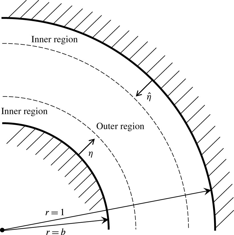
In this limit, the viscous diffusion thickness is very small. The vorticity is confined to narrow Stokes layers on the two boundaries. The space between the two spheres can be divided into three regions: the inner region around the inner sphere, the inner region around the container, and the outer region which is the bulk of the annular region. We have depicted a schematic of the different regions in figure 1.
A schematic of the streaming flow regions at high frequency.

2.5.1 The oscillating field
First we consider the inner region, which is the boundary layer around the inner sphere. The inner variables with the Stokes layers are scaled as follows:
 $$\begin{eqnarray}\unicode[STIX]{x1D702}=(r-b)\frac{|M|}{\sqrt{2}}\quad \text{and}\quad \unicode[STIX]{x1D6F9}=\unicode[STIX]{x1D713}\frac{|M|}{\sqrt{2}}.\end{eqnarray}$$
As a result, the governing equations become
 $$\begin{eqnarray}\displaystyle & & \displaystyle \frac{\unicode[STIX]{x2202}}{\unicode[STIX]{x2202}t}\left(\frac{\unicode[STIX]{x2202}^{2}\unicode[STIX]{x1D6F9}}{\unicode[STIX]{x2202}\unicode[STIX]{x1D702}^{2}}\right)+\frac{\unicode[STIX]{x1D700}}{b^{2}}\left[\frac{\unicode[STIX]{x2202}\displaystyle \displaystyle \left(\unicode[STIX]{x1D6F9},\frac{\unicode[STIX]{x2202}^{2}\unicode[STIX]{x1D6F9}}{\unicode[STIX]{x2202}\unicode[STIX]{x1D702}^{2}}\right)}{\unicode[STIX]{x2202}(\unicode[STIX]{x1D702},\unicode[STIX]{x1D707})}+2\frac{\unicode[STIX]{x1D707}}{(1-\unicode[STIX]{x1D707}^{2})}\frac{\unicode[STIX]{x2202}\unicode[STIX]{x1D6F9}}{\unicode[STIX]{x2202}\unicode[STIX]{x1D702}}\frac{\unicode[STIX]{x2202}^{2}\unicode[STIX]{x1D6F9}}{\unicode[STIX]{x2202}\unicode[STIX]{x1D702}^{2}}+2\frac{\unicode[STIX]{x1D707}}{(1-\unicode[STIX]{x1D707}^{2})}\unicode[STIX]{x1D6FA}\frac{\unicode[STIX]{x2202}\unicode[STIX]{x1D6FA}}{\unicode[STIX]{x2202}\unicode[STIX]{x1D702}}\right]\nonumber\\ \displaystyle & & \displaystyle \quad =\frac{1}{2}\frac{\unicode[STIX]{x2202}^{4}\unicode[STIX]{x1D6F9}}{\unicode[STIX]{x2202}\unicode[STIX]{x1D702}^{4}},\end{eqnarray}$$
 $$\begin{eqnarray}\displaystyle \frac{\unicode[STIX]{x2202}\unicode[STIX]{x1D6FA}}{\unicode[STIX]{x2202}t}+\frac{\unicode[STIX]{x1D700}}{b^{2}}\left[\frac{\unicode[STIX]{x2202}(\unicode[STIX]{x1D6F9},\unicode[STIX]{x1D6FA})}{\unicode[STIX]{x2202}(\unicode[STIX]{x1D702},\unicode[STIX]{x1D707})}\right]=\frac{1}{2}\frac{\unicode[STIX]{x2202}^{2}\unicode[STIX]{x1D6FA}}{\unicode[STIX]{x2202}\unicode[STIX]{x1D702}^{2}}, & & \displaystyle\end{eqnarray}$$
with boundary conditions
 $$\begin{eqnarray}\displaystyle & \displaystyle \frac{\unicode[STIX]{x2202}\unicode[STIX]{x1D6F9}}{\unicode[STIX]{x2202}\unicode[STIX]{x1D707}}=-b^{2}\frac{|M|}{\sqrt{2}}\unicode[STIX]{x1D707}\sin t,\quad \frac{\unicode[STIX]{x2202}\unicode[STIX]{x1D6F9}}{\unicode[STIX]{x2202}\unicode[STIX]{x1D702}}=b(1-\unicode[STIX]{x1D707}^{2})\sin t, & \displaystyle \nonumber\\ \displaystyle & \displaystyle \text{and}\quad \unicode[STIX]{x1D6FA}=b\unicode[STIX]{x1D6FC}(1-\unicode[STIX]{x1D707}^{2})\sin (t+\unicode[STIX]{x1D6FD})\quad \text{on }\unicode[STIX]{x1D702}=0. & \displaystyle\end{eqnarray}$$
 $\unicode[STIX]{x1D6F9}$
and
 $\unicode[STIX]{x1D6FA}$
can be expressed as
 $$\begin{eqnarray}\displaystyle \unicode[STIX]{x1D6F9} & = & \displaystyle \unicode[STIX]{x1D6F9}_{0}+\unicode[STIX]{x1D700}\unicode[STIX]{x1D6F9}_{1}+O(\unicode[STIX]{x1D700}^{2}),\end{eqnarray}$$
 $$\begin{eqnarray}\displaystyle \unicode[STIX]{x1D6FA} & = & \displaystyle \unicode[STIX]{x1D6FA}_{0}+\unicode[STIX]{x1D700}\unicode[STIX]{x1D6FA}_{1}+O(\unicode[STIX]{x1D700}^{2}).\end{eqnarray}$$
 $$\begin{eqnarray}\displaystyle & \displaystyle \frac{\unicode[STIX]{x2202}}{\unicode[STIX]{x2202}t}\left(\frac{\unicode[STIX]{x2202}^{2}\unicode[STIX]{x1D6F9}_{0}}{\unicode[STIX]{x2202}\unicode[STIX]{x1D702}^{2}}\right)=\frac{1}{2}\frac{\unicode[STIX]{x2202}^{4}\unicode[STIX]{x1D6F9}_{0}}{\unicode[STIX]{x2202}\unicode[STIX]{x1D702}^{4}}, & \displaystyle\end{eqnarray}$$
 $$\begin{eqnarray}\displaystyle & \displaystyle \frac{\unicode[STIX]{x2202}\unicode[STIX]{x1D6FA}_{0}}{\unicode[STIX]{x2202}t}=\frac{1}{2}\frac{\unicode[STIX]{x2202}^{2}\unicode[STIX]{x1D6FA}_{0}}{\unicode[STIX]{x2202}\unicode[STIX]{x1D702}^{2}}. & \displaystyle\end{eqnarray}$$
 $$\begin{eqnarray}\displaystyle \unicode[STIX]{x1D6F9}_{0} & = & \displaystyle \left\{a_{0}\text{e}^{-(1+\text{i})\unicode[STIX]{x1D702}}+\left[\frac{b}{2\text{i}}+(1+\text{i})a_{0}\right]\unicode[STIX]{x1D702}+\frac{|M|}{4\sqrt{2}i}b^{2}-a_{0}\right\}(1-\unicode[STIX]{x1D707}^{2})\text{e}^{\text{i}t}+\text{c.c.},\hspace{24.0pt}\end{eqnarray}$$
 $$\begin{eqnarray}\displaystyle \unicode[STIX]{x1D6FA}_{0} & = & \displaystyle \frac{\unicode[STIX]{x1D6FC}b}{2\text{i}}(1-\unicode[STIX]{x1D707}^{2})\text{e}^{-(1+\text{i})\unicode[STIX]{x1D702}}\text{e}^{\text{i}(t+\unicode[STIX]{x1D6FD})}+\text{c.c.}\end{eqnarray}$$
Next, we have two equations for the outer region,
 $$\begin{eqnarray}\displaystyle \frac{\unicode[STIX]{x2202}}{\unicode[STIX]{x2202}t}(\text{D}^{2}\unicode[STIX]{x1D713}_{0}) & = & \displaystyle 0,\end{eqnarray}$$
 $$\begin{eqnarray}\displaystyle \frac{\unicode[STIX]{x2202}\unicode[STIX]{x1D6FA}_{0}}{\unicode[STIX]{x2202}t} & = & \displaystyle 0.\end{eqnarray}$$
 $$\begin{eqnarray}\displaystyle \unicode[STIX]{x1D713}_{0} & = & \displaystyle \left(a_{0}^{\ast }r^{2}+b_{0}^{\ast }\frac{1}{r}\right)(1-\unicode[STIX]{x1D707}^{2})\text{e}^{\text{i}t}+\text{c.c.},\end{eqnarray}$$
 $$\begin{eqnarray}\displaystyle \unicode[STIX]{x1D6FA}_{0} & = & \displaystyle 0.\end{eqnarray}$$
Finally, in the boundary layer on the container, with boundary-layer variables introduced as
 $$\begin{eqnarray}\hat{\unicode[STIX]{x1D702}}=(1-r)\frac{|M|}{\sqrt{2}}\quad \text{and}\quad \bar{\unicode[STIX]{x1D6F9}}=\unicode[STIX]{x1D713}\frac{|M|}{\sqrt{2}},\end{eqnarray}$$
the governing equations become
 $$\begin{eqnarray}\displaystyle & \displaystyle \!\!\frac{\unicode[STIX]{x2202}}{\unicode[STIX]{x2202}t}\left(\frac{\unicode[STIX]{x2202}^{2}\bar{\unicode[STIX]{x1D6F9}}}{\unicode[STIX]{x2202}\hat{\unicode[STIX]{x1D702}}^{2}}\right)-\unicode[STIX]{x1D700}\left[\frac{\unicode[STIX]{x2202}\displaystyle \left(\bar{\unicode[STIX]{x1D6F9}},\frac{\unicode[STIX]{x2202}^{2}\bar{\unicode[STIX]{x1D6F9}}}{\unicode[STIX]{x2202}\hat{\unicode[STIX]{x1D702}}^{2}}\right)}{\unicode[STIX]{x2202}(\hat{\unicode[STIX]{x1D702}},\unicode[STIX]{x1D707})}+2\frac{\unicode[STIX]{x1D707}}{(1-\unicode[STIX]{x1D707}^{2})}\frac{\unicode[STIX]{x2202}\bar{\unicode[STIX]{x1D6F9}}}{\unicode[STIX]{x2202}\hat{\unicode[STIX]{x1D702}}}\frac{\unicode[STIX]{x2202}^{2}\bar{\unicode[STIX]{x1D6F9}}}{\unicode[STIX]{x2202}\hat{\unicode[STIX]{x1D702}}^{2}}+2\frac{\unicode[STIX]{x1D707}}{(1-\unicode[STIX]{x1D707}^{2})}\unicode[STIX]{x1D6FA}\frac{\unicode[STIX]{x2202}\unicode[STIX]{x1D6FA}}{\unicode[STIX]{x2202}\hat{\unicode[STIX]{x1D702}}}\right]=\frac{1}{2}\frac{\unicode[STIX]{x2202}^{4}\bar{\unicode[STIX]{x1D6F9}}}{\unicode[STIX]{x2202}\hat{\unicode[STIX]{x1D702}}^{4}}, & \displaystyle \nonumber\\ \displaystyle & & \displaystyle\end{eqnarray}$$
 $$\begin{eqnarray}\displaystyle & \displaystyle \frac{\unicode[STIX]{x2202}\unicode[STIX]{x1D6FA}}{\unicode[STIX]{x2202}t}-\unicode[STIX]{x1D700}\left[\frac{\unicode[STIX]{x2202}(\bar{\unicode[STIX]{x1D6F9}},\unicode[STIX]{x1D6FA})}{\unicode[STIX]{x2202}(\hat{\unicode[STIX]{x1D702}},\unicode[STIX]{x1D707})}\right]=\frac{1}{2}\frac{\unicode[STIX]{x2202}^{2}\unicode[STIX]{x1D6FA}}{\unicode[STIX]{x2202}\hat{\unicode[STIX]{x1D702}}^{2}}, & \displaystyle\end{eqnarray}$$
 $$\begin{eqnarray}\hat{\unicode[STIX]{x1D702}}=0,\quad \bar{\unicode[STIX]{x1D6F9}}=\frac{\unicode[STIX]{x2202}\bar{\unicode[STIX]{x1D6F9}}}{\unicode[STIX]{x2202}\hat{\unicode[STIX]{x1D702}}}=\unicode[STIX]{x1D6FA}=0.\end{eqnarray}$$
After the perturbation method is applied, solutions to order
 $O(1)$
in the boundary layer on the container are
 $$\begin{eqnarray}\displaystyle \bar{\unicode[STIX]{x1D6F9}}_{0} & = & \displaystyle d_{0}[\text{e}^{-(1+\text{i})\hat{\unicode[STIX]{x1D702}}}+(1+\text{i})\hat{\unicode[STIX]{x1D702}}-1](1-\unicode[STIX]{x1D707}^{2})\text{e}^{\text{i}t}+\text{c.c.},\end{eqnarray}$$
 $$\begin{eqnarray}\displaystyle \unicode[STIX]{x1D6FA}_{0} & = & \displaystyle 0.\end{eqnarray}$$
The coefficients in the solutions of each region are yet undetermined and can be obtained later by matching with the solutions in other regions next to them, according to the requirements
 $$\begin{eqnarray}\displaystyle & \displaystyle \unicode[STIX]{x1D6F9}_{0}|_{\unicode[STIX]{x1D702}\rightarrow \infty }=\frac{|M|}{\sqrt{2}}\unicode[STIX]{x1D713}_{0}|_{r\rightarrow b}, & \displaystyle\end{eqnarray}$$
 $$\begin{eqnarray}\displaystyle & \displaystyle \bar{\unicode[STIX]{x1D6F9}}_{0}|_{\hat{\unicode[STIX]{x1D702}}\rightarrow \infty }=\frac{|M|}{\sqrt{2}}\unicode[STIX]{x1D713}_{0}|_{r\rightarrow 1}. & \displaystyle\end{eqnarray}$$
 $$\begin{eqnarray}\displaystyle \unicode[STIX]{x1D713}_{0} & = & \displaystyle -\frac{1}{4\text{i}}\left(\frac{b^{3}}{1-b^{3}}\right)\left(r^{2}-\frac{1}{r}\right)(1-\unicode[STIX]{x1D707}^{2})\text{e}^{\text{i}t}+\text{c.c.},\end{eqnarray}$$
 $$\begin{eqnarray}\displaystyle \unicode[STIX]{x1D6FA}_{0} & = & \displaystyle 0.\end{eqnarray}$$
 $$\begin{eqnarray}\displaystyle \unicode[STIX]{x1D6F9}_{0} & = & \displaystyle \left\{\frac{3(1+\text{i})}{8}\left(\frac{b}{1-b^{3}}\right)[\text{e}^{-(1+\text{i})(|M|/\sqrt{2})(r-b)}-1]+\frac{|M|}{4\sqrt{2}}\text{i}\left[\frac{2b^{4}+b}{1-b^{3}}(r-b)-b^{2}\right]\right\}\nonumber\\ \displaystyle & & \displaystyle \times \,(1-\unicode[STIX]{x1D707}^{2})\text{e}^{\text{i}t}+\text{c.c.},\end{eqnarray}$$
 $$\begin{eqnarray}\displaystyle \unicode[STIX]{x1D6FA}_{0} & = & \displaystyle \frac{\unicode[STIX]{x1D6FC}b}{2\text{i}}\text{e}^{-(1+\text{i})(|M|/\sqrt{2})(r-b)}(1-\unicode[STIX]{x1D707}^{2})\text{e}^{\text{i}(t+\unicode[STIX]{x1D6FD})}+\text{c.c.}\end{eqnarray}$$
 $$\begin{eqnarray}\displaystyle \bar{\unicode[STIX]{x1D6F9}}_{0} & = & \displaystyle -\frac{3(1+\text{i})}{8}\frac{b^{3}}{1-b^{3}}\left[\text{e}^{-(1+\text{i})(|M|/\sqrt{2})(1-r)}+(1+\text{i})\frac{|M|}{\sqrt{2}}(1-r)-1\right](1-\unicode[STIX]{x1D707}^{2})\text{e}^{\text{i}t}+\text{c.c.},\nonumber\\ \displaystyle & & \displaystyle\end{eqnarray}$$
 $$\begin{eqnarray}\displaystyle \unicode[STIX]{x1D6FA}_{0} & = & \displaystyle 0.\end{eqnarray}$$
 $$\begin{eqnarray}\displaystyle \unicode[STIX]{x1D713}_{0} & = & \displaystyle \left[\frac{\sqrt{2}}{|M|}\frac{3(1+\text{i})}{8}\left(\frac{b}{1-b^{3}}\right)\text{e}^{-(1+\text{i})(|M|/\sqrt{2})(r-b)}\right.\nonumber\\ \displaystyle & & \displaystyle -\,\frac{\sqrt{2}}{|M|}\frac{3(1+\text{i})}{8}\left(\frac{b}{1-b^{3}}\right)\text{e}^{-(1+\text{i})(|M|/\sqrt{2})(1-r)}\nonumber\\ \displaystyle & & \displaystyle \left.-\,\frac{1}{4\text{i}}\left(\frac{b^{3}}{1-b^{3}}\right)\left(r^{2}-\frac{1}{r}\right)\right](1-\unicode[STIX]{x1D707}^{2})\text{e}^{\text{i}t}+\text{c.c.},\end{eqnarray}$$
 $$\begin{eqnarray}\displaystyle \unicode[STIX]{x1D6FA}_{0} & = & \displaystyle \frac{\unicode[STIX]{x1D6FC}b}{2\text{i}}\text{e}^{-(1+\text{i})(|M|/\sqrt{2})(r-b)}(1-\unicode[STIX]{x1D707}^{2})\text{e}^{\text{i}(t+\unicode[STIX]{x1D6FD})}+\text{c.c.},\end{eqnarray}$$
 $$\begin{eqnarray}\displaystyle \unicode[STIX]{x1D70F}_{0r\unicode[STIX]{x1D703}} & = & \displaystyle \left\{\frac{3}{4}\left(\frac{b}{1-b^{3}}\right)\left[-\frac{2\text{i}}{r^{2}}-(1+\text{i})\frac{\sqrt{2}}{|M|}\frac{1}{r^{3}}+(1-\text{i})\frac{|M|}{\sqrt{2}}\frac{1}{r}\right]\text{e}^{-(1+\text{i})(|M|/\sqrt{2})(r-b)}\right.\nonumber\\ \displaystyle & & \displaystyle +\,\frac{3}{4}\left(\frac{b}{1-b^{3}}\right)\left[-\frac{2\text{i}}{r^{2}}+(1+\text{i})\frac{\sqrt{2}}{|M|}\frac{1}{r^{3}}-(1-\text{i})\frac{|M|}{\sqrt{2}}\frac{1}{r}\right]\text{e}^{-(1+\text{i})(|M|/\sqrt{2})(1-r)}\nonumber\\ \displaystyle & & \displaystyle \left.-\,\frac{3}{2\text{i}}\left(\frac{b^{3}}{1-b^{3}}\right)\frac{1}{r^{4}}\right\}(1-\unicode[STIX]{x1D707}^{2})^{1/2}\text{e}^{\text{i}t}+\text{c.c.},\end{eqnarray}$$
 $$\begin{eqnarray}\displaystyle \unicode[STIX]{x1D70F}_{0r\unicode[STIX]{x1D719}} & = & \displaystyle \frac{\unicode[STIX]{x1D6FC}b\text{e}^{\text{i}\unicode[STIX]{x1D6FD}}}{2\text{i}}\left[-\frac{2}{r^{2}}-(1+\text{i})\frac{|M|}{\sqrt{2}}\frac{1}{r}\right]\text{e}^{-(1+\text{i})(|M|/\sqrt{2})(r-b)}(1-\unicode[STIX]{x1D707}^{2})^{1/2}\text{e}^{\text{i}t}+\text{c.c.},\nonumber\\ \displaystyle & & \displaystyle\end{eqnarray}$$
 $$\begin{eqnarray}\displaystyle \unicode[STIX]{x1D70F}_{0\unicode[STIX]{x1D719}\unicode[STIX]{x1D703}} & = & \displaystyle 0.\end{eqnarray}$$
2.5.2 Steady streaming
Similarly, to order
 $\unicode[STIX]{x1D700}$
, the streaming is still studied separately in three regions, and then solutions are matched to determine the coefficients in those solutions. Specifically, in the outer region, the steady flow is characterized by the streaming Reynolds number, which is defined as
 $$\begin{eqnarray}R_{s}=\frac{U_{0}^{2}}{\unicode[STIX]{x1D714}\unicode[STIX]{x1D708}}=\unicode[STIX]{x1D700}^{2}|M|^{2}=\left(\frac{\text{Displacement amplitude of torsional oscillation}}{\text{Stokes-layer thickness}}\right)^{2}.\end{eqnarray}$$
This is not an independent parameter, because it is determined by
 $\unicode[STIX]{x1D700}$
and
 $|M|$
together. Here, only
 $R_{s}\ll 1$
is considered, in which case the governing equation is the Stokes equation.
Then, according to the matching requirement similar to (2.42), solutions in three regions are obtained with all the coefficients determined, and the composite solutions can be written as (see appendix A for procedures)
 $$\begin{eqnarray}\displaystyle \unicode[STIX]{x1D713}_{1}^{(s)} & = & \displaystyle \left\{\frac{\sqrt{2}}{|M|}\left(\frac{2}{b^{2}}\right)\left[-\frac{3}{4}\left(\frac{\text{i}}{4}\frac{|M|}{\sqrt{2}}b^{2}+(1+\text{i})b-\frac{3(5+3\text{i})}{8}\left(\frac{b}{1-b^{3}}\right)\right)\frac{b}{1-b^{3}}\right.\right.\nonumber\\ \displaystyle & & \displaystyle \times \,\text{e}^{-(1+\text{i})(|M|/\sqrt{2})(r-b)}+\frac{1+\text{i}}{32}\left(\frac{9}{4}\left(\frac{b}{1-b^{3}}\right)^{2}-(\unicode[STIX]{x1D6FC}b)^{2}\right)\text{e}^{-2(|M|/\sqrt{2})(r-b)}\nonumber\\ \displaystyle & & \displaystyle \left.\times \,\frac{3\text{i}}{8}\frac{|M|}{\sqrt{2}}\left(b-\frac{3}{2}\left(\frac{b}{1-b^{3}}\right)\right)\frac{b}{1-b^{3}}(r-b)\text{e}^{-(1+\text{i})(|M|/\sqrt{2})(r-b)}\right]\nonumber\\ \displaystyle & & \displaystyle -\,\frac{\sqrt{2}}{|M|}\left(\frac{9b^{6}}{8(1-b^{3})^{2}}\right)\left[\frac{1+\text{i}}{8}\text{e}^{-2(|M|/\sqrt{2})(1-r)}+\frac{5+3\text{i}}{2}\text{e}^{-(1+\text{i})(|M|/\sqrt{2})(1-r)}\right.\nonumber\\ \displaystyle & & \displaystyle \left.\left.+\,\text{i}\frac{|M|}{\sqrt{2}}(1-r)\text{e}^{-(1+\text{i})(|M|/\sqrt{2})(1-r)}\right]+\left(A_{3}r^{5}+B_{3}r^{3}+C_{3}+\frac{D_{3}}{r^{2}}\right)\right\}\nonumber\\ \displaystyle & & \displaystyle \times \,\unicode[STIX]{x1D707}(1-\unicode[STIX]{x1D707}^{2})+\text{c.c.},\end{eqnarray}$$
 $$\begin{eqnarray}\displaystyle \unicode[STIX]{x1D6FA}_{1}^{(s)} & = & \displaystyle \left\{\frac{2\unicode[STIX]{x1D6FC}\text{e}^{\text{i}\unicode[STIX]{x1D6FD}}}{b}\left[-\frac{3(1-\text{i})}{16}\left(\frac{b}{1-b^{3}}\right)\text{e}^{-2(|M|/\sqrt{2})(r-b)}+\frac{1}{4}\left(-\frac{(1-\text{i})}{2}\frac{|M|}{\sqrt{2}}b^{2}+3\text{i}b\right.\right.\right.\nonumber\\ \displaystyle & & \displaystyle \left.-\,\frac{3(1+3\text{i})}{2}\left(\frac{b}{1-b^{3}}\right)\right)\text{e}^{-(1+\text{i})(|M|/\sqrt{2})(r-b)}\nonumber\\ \displaystyle & & \displaystyle -\,\frac{(1-\text{i})}{4}\frac{|M|}{\sqrt{2}}\left(b-\frac{3}{2}\left(\frac{b}{1-b^{3}}\right)\right)(r-b)\nonumber\\ \displaystyle & & \displaystyle \left.\left.\times \,\text{e}^{-(1+\text{i})(|M|/\sqrt{2})(r-b)}\right]+A_{3}^{\ast }r^{3}+\frac{B_{3}^{\ast }}{r^{2}}\right\}\unicode[STIX]{x1D707}(1-\unicode[STIX]{x1D707}^{2})+\text{c.c.},\end{eqnarray}$$
 $$\begin{eqnarray}\displaystyle u_{1r}^{(s)} & = & \displaystyle \left\{\frac{\sqrt{2}}{|M|}\left(\frac{2}{b^{2}r^{2}}\right)\left[-\frac{3}{4}\left(\frac{\text{i}}{4}\frac{|M|}{\sqrt{2}}b^{2}+(1+\text{i})b-\frac{3(5+3\text{i})}{8}\left(\frac{b}{1-b^{3}}\right)\right)\frac{b}{1-b^{3}}\right.\right.\nonumber\\ \displaystyle & & \displaystyle \qquad \times \,\text{e}^{-(1+\text{i})(|M|/\sqrt{2})(r-b)}+\frac{1+\text{i}}{32}\left(\frac{9}{4}\left(\frac{b}{1-b^{3}}\right)^{2}-(\unicode[STIX]{x1D6FC}b)^{2}\right)\text{e}^{-2(|M|/\sqrt{2})(r-b)}\nonumber\\ \displaystyle & & \displaystyle \left.-\,\frac{3\text{i}}{8}\frac{|M|}{\sqrt{2}}\left(b-\frac{3}{2}\left(\frac{b}{1-b^{3}}\right)\right)\frac{b}{1-b^{3}}(r-b)\text{e}^{-(1+\text{i})(|M|/\sqrt{2})(r-b)}\right]\nonumber\\ \displaystyle & & \displaystyle -\,\frac{\sqrt{2}}{|M|}\left(\frac{9b^{6}}{8(1-b^{3})^{2}}\right)\frac{1}{r^{2}}\left[\frac{1+\text{i}}{8}\text{e}^{-2(|M|/\sqrt{2})(1-r)}+\frac{5+3\text{i}}{2}\text{e}^{-(1+\text{i})(|M|/\sqrt{2})(1-r)}\right.\nonumber\\ \displaystyle & & \displaystyle \left.\left.+\,\text{i}\frac{|M|}{\sqrt{2}}(1-r)\text{e}^{-(1+\text{i})(|M|/\sqrt{2})(1-r)}\right]+\left(A_{3}r^{3}+B_{3}r+\frac{C_{3}}{r^{2}}+\frac{D_{3}}{r^{4}}\right)\right\}\nonumber\\ \displaystyle & & \displaystyle \times \,(3\unicode[STIX]{x1D707}^{2}-1)+\text{c.c.},\end{eqnarray}$$
 $$\begin{eqnarray}\displaystyle u_{1\unicode[STIX]{x1D703}}^{(s)} & = & \displaystyle \left\{\frac{2}{b^{2}r}\left[-\frac{3}{8}\left(-\frac{(1-\text{i})}{2}\frac{|M|}{\sqrt{2}}b^{2}+3\text{i}b-\frac{3(1+3\text{i})}{2}\left(\frac{b}{1-b^{3}}\right)\right)\frac{b}{1-b^{3}}\right.\right.\nonumber\\ \displaystyle & & \displaystyle \times \,\text{e}^{-(1+\text{i})(|M|/\sqrt{2})(r-b)}+\frac{1+\text{i}}{16}\left(\frac{9}{4}\left(\frac{b}{1-b^{3}}\right)^{2}-(\unicode[STIX]{x1D6FC}b)^{2}\right)\text{e}^{-2(|M|/\sqrt{2})(r-b)}\nonumber\\ \displaystyle & & \displaystyle \left.+\,\frac{3(1-\text{i})}{8}\frac{|M|}{\sqrt{2}}\left(b-\frac{3}{2}\left(\frac{b}{1-b^{3}}\right)\right)\frac{b}{1-b^{3}}(r-b)\text{e}^{-(1+\text{i})(|M|/\sqrt{2})(r-b)}\right]\nonumber\\ \displaystyle & & \displaystyle +\,\frac{9b^{6}}{8(1-b^{3})^{2}}\frac{1}{r}\left[\frac{1+\text{i}}{4}\text{e}^{-2(|M|/\sqrt{2})(1-r)}+(1+3\text{i})\text{e}^{-(1+\text{i})(|M|/\sqrt{2})(1-r)}\right.\nonumber\\ \displaystyle & & \displaystyle \left.\left.-\,(1-\text{i})\frac{|M|}{\sqrt{2}}(1-r)\text{e}^{-(1+\text{i})(|M|/\sqrt{2})(1-r)}\right]+\left(-5A_{3}r^{3}-3B_{3}r+2\frac{D_{3}}{r^{4}}\right)\right\}\nonumber\\ \displaystyle & & \displaystyle \times \,\unicode[STIX]{x1D707}(1-\unicode[STIX]{x1D707}^{2})^{1/2}+\text{c.c.},\end{eqnarray}$$
 $$\begin{eqnarray}\displaystyle u_{1\unicode[STIX]{x1D719}}^{(s)} & = & \displaystyle \left\{\frac{2\unicode[STIX]{x1D6FC}\text{e}^{\text{i}\unicode[STIX]{x1D6FD}}}{br}\left[-\frac{3(1-\text{i})}{16}\left(\frac{b}{1-b^{3}}\right)\text{e}^{-2(|M|/\sqrt{2})(r-b)}+\frac{1}{4}\left(-\frac{(1-\text{i})}{2}\frac{|M|}{\sqrt{2}}b^{2}+3\text{i}b\right.\right.\right.\nonumber\\ \displaystyle & & \displaystyle \left.-\,\frac{3(1+3\text{i})}{2}\left(\frac{b}{1-b^{3}}\right)\right)\text{e}^{-(1+\text{i})(|M|/\sqrt{2})(r-b)}\nonumber\\ \displaystyle & & \displaystyle -\,\frac{(1-\text{i})}{4}\frac{|M|}{\sqrt{2}}\left(b-\frac{3}{2}\left(\frac{b}{1-b^{3}}\right)\right)(r-b)\nonumber\\ \displaystyle & & \displaystyle \left.\left.\times \,\text{e}^{-(1+\text{i})(|M|/\sqrt{2})(r-b)}\right]+A_{3}^{\ast }r^{2}+\frac{B_{3}^{\ast }}{r^{3}}\right\}\unicode[STIX]{x1D707}(1-\unicode[STIX]{x1D707}^{2})^{1/2}+\text{c.c.},\end{eqnarray}$$
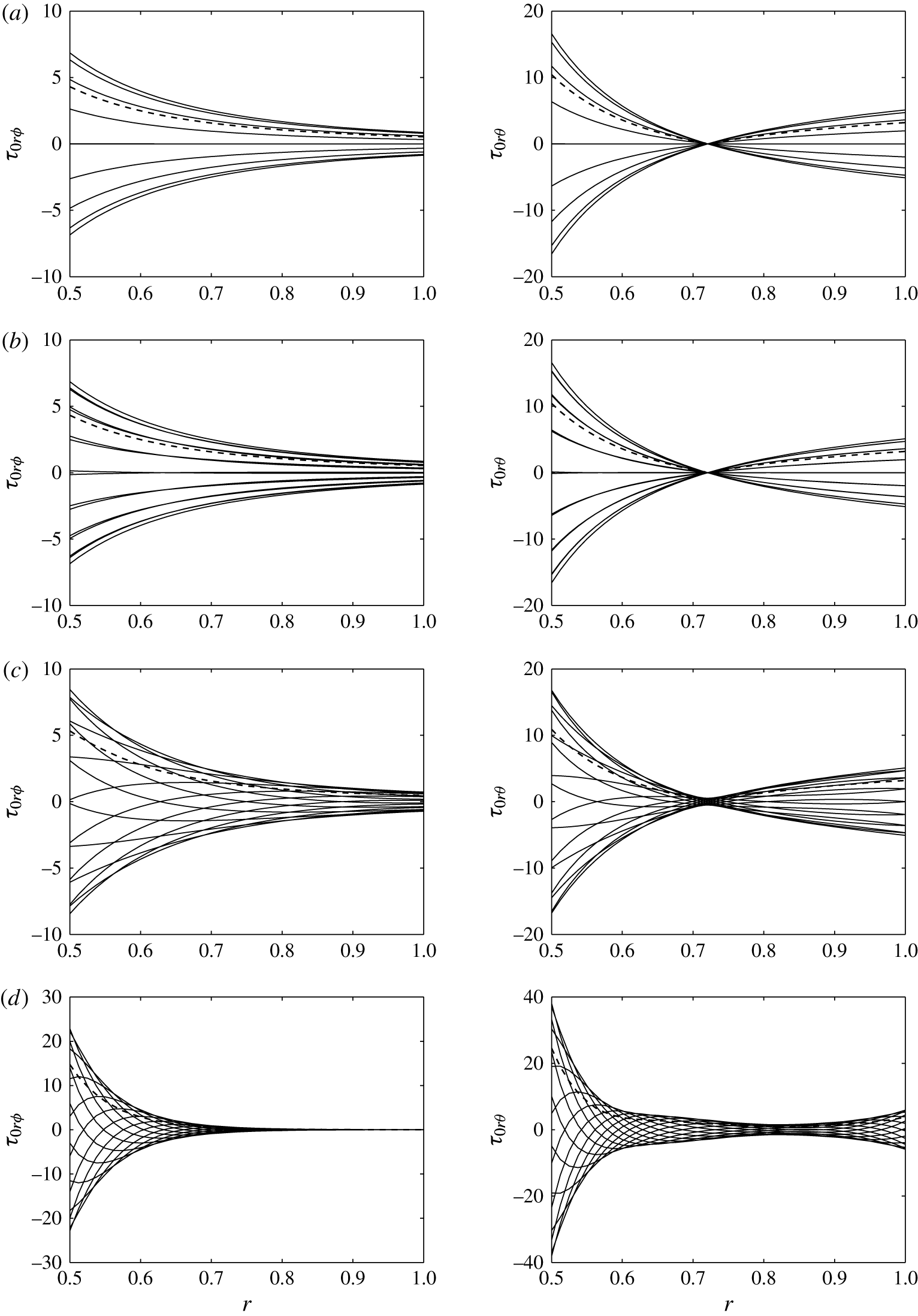
Leading-order shear stress profiles on the equatorial plane over one time period with
 $b=0.5$
,
 $\unicode[STIX]{x1D6FC}=1$
and
 $\unicode[STIX]{x1D6FD}=\unicode[STIX]{x03C0}/4$
. The dashed curve shows the time average of absolute shear stress values over one period. (a)
 $|M|\ll 1$
, (b)
 $|M|=1$
, (c)
 $|M|=5$
, (d)
 $|M|=20$
.

3 Results
In figure 2, the leading-order shear stress profiles under different values of the Womersley number
 $|M|$
are investigated. According to (2.12), transverse oscillations result in the leading-order shear stress
 $\unicode[STIX]{x1D70F}_{0r\unicode[STIX]{x1D703}}$
, while torsional oscillations result in
 $\unicode[STIX]{x1D70F}_{0r\unicode[STIX]{x1D719}}$
. It means that for combined oscillation, the graphs for leading-order shear stress components are the same as those for transverse or torsional oscillation only, as in our previous work (Kong, Penkova & Sadhal Reference Kong, Penkova and Sadhal2015). Also, for both shear stresses, the maximum values can be found on the inner boundary. These maximum values rise with increasing Womersley number
 $|M|$
. As
 $|M|$
increases to 20, torsional oscillations can lead to shear stress
 $\unicode[STIX]{x1D70F}_{0r\unicode[STIX]{x1D719}}$
mainly close to the inner boundary, while the value of
 $\unicode[STIX]{x1D70F}_{0r\unicode[STIX]{x1D719}}$
is quite small for the outside part of the region. In contrast, influence of transverse oscillation on shear stress
 $\unicode[STIX]{x1D70F}_{0r\unicode[STIX]{x1D703}}$
close to the outer boundary remains the same as
 $|M|$
rises, as can be seen from the shear stress value on the outer boundary. Especially for low-frequency
 $(|M|\ll 1)$
, the shear stress profiles, shown in figure 2(a), are similar to those for
 $|M|=1$
in figure 2(b). At low frequency, a reduction of the Womersley number
 $|M|$
does not cause a significant decrease in shear stress values.
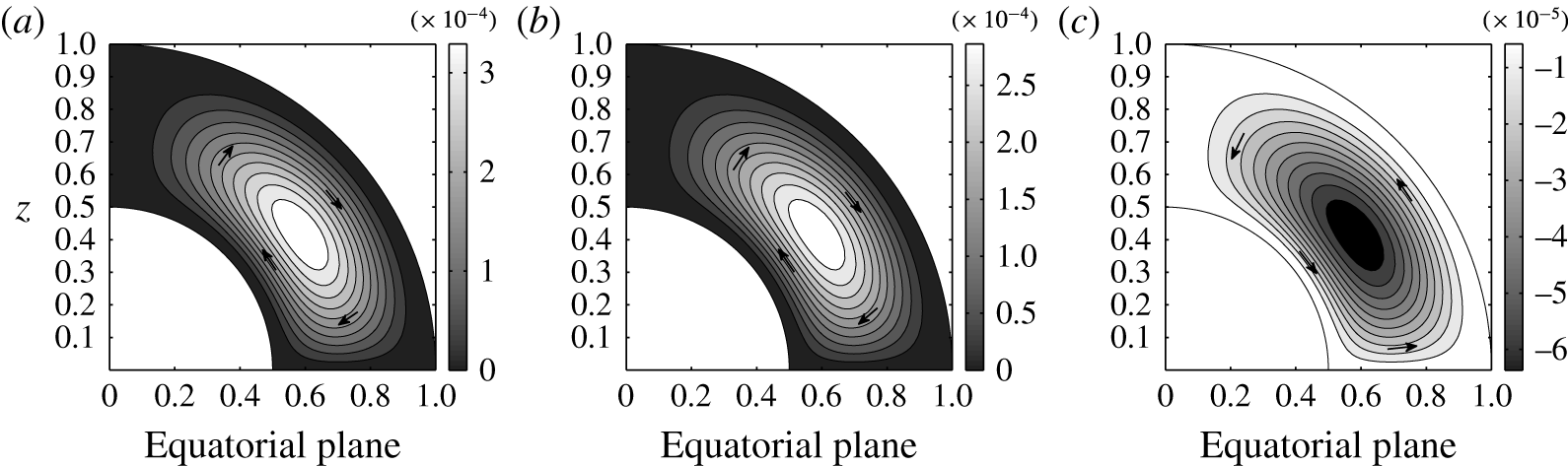
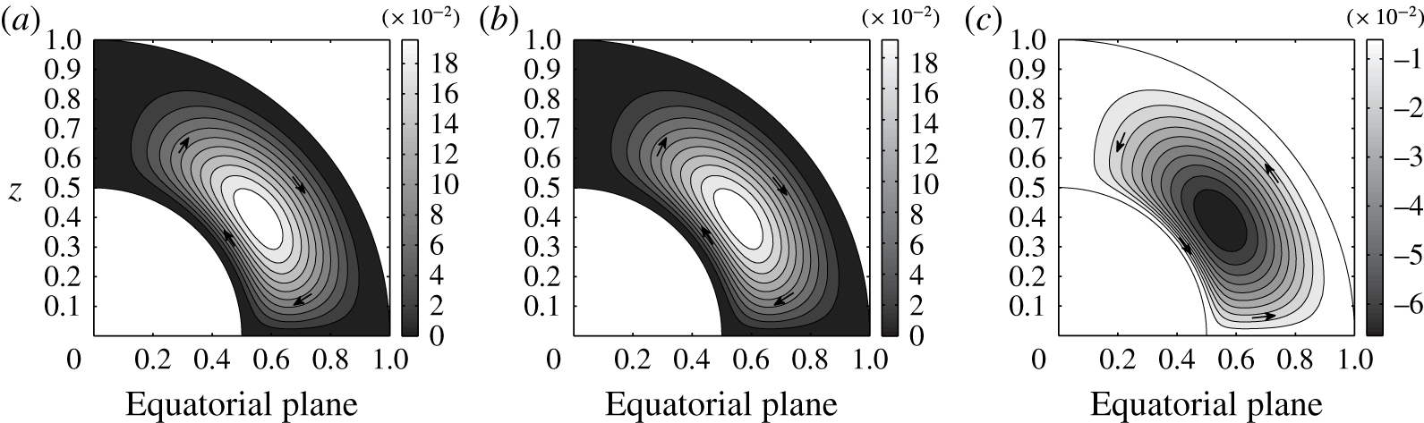
The streaming flow pattern on
 $r$
–
 $\unicode[STIX]{x1D703}$
plane for low frequency under different amplitude ratio with
 $b=0.5$
. (a)
 $\unicode[STIX]{x1D6FC}=0$
, (b)
 $\unicode[STIX]{x1D6FC}=1$
, (c)
 $\unicode[STIX]{x1D6FC}=3$
.

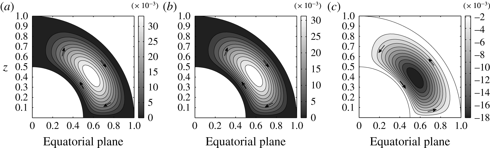
The streaming flow pattern on
 $r$
–
 $\unicode[STIX]{x1D703}$
plane for
 $|M|=10$
under different amplitude ratio with
 $b=0.5$
. (a)
 $\unicode[STIX]{x1D6FC}=0$
, (b)
 $\unicode[STIX]{x1D6FC}=1$
, (c)
 $\unicode[STIX]{x1D6FC}=5$
.

The streaming flow pattern on
 $r$
–
 $\unicode[STIX]{x1D703}$
plane for high frequency
 $(|M|=25)$
under different amplitude ratio with
 $b=0.5$
. (a)
 $\unicode[STIX]{x1D6FC}=0$
, (b)
 $\unicode[STIX]{x1D6FC}=1$
, (c)
 $\unicode[STIX]{x1D6FC}=8$
.

Kong et al. (Reference Kong, Penkova and Sadhal2015) showed that second-order steady streaming, induced by a single transverse or torsional oscillation, is only on the
 $r$
–
 $\unicode[STIX]{x1D703}$
plane. For transverse oscillation only, the streaming vortex in the first quadrant on the
 $\unicode[STIX]{x1D719}=0$
plane is clockwise, and counter-clockwise for torsional oscillation only. However, for superposed transverse and torsional oscillations, the azimuthal velocity of steady streaming is non-zero. Steady streaming patterns at low frequency for different values of the amplitude ratio
 $\unicode[STIX]{x1D6FC}$
are plotted in figure 3 (for
 $|M|=10$
in figure 4, and for high frequency in figure 5). The vortices of streaming for only transverse oscillation
 $(\unicode[STIX]{x1D6FC}=0)$
, shown in figures 3(a), 4(a) and 5(a), are the same as those in Kong et al. (Reference Kong, Penkova and Sadhal2015). As
 $\unicode[STIX]{x1D6FC}$
is increased, the effect of torsional oscillations is enhanced. We take low frequency for example. As the ratio of amplitude
 $\unicode[STIX]{x1D6FC}$
goes up from 1 to 3, the vortex changes direction from clockwise to counter-clockwise in the first quadrant on the
 $\unicode[STIX]{x1D719}=0$
plane. This transition takes place at a value of
 $\unicode[STIX]{x1D6FC}$
between 2 and 3. On the other hand, for
 $|M|=10$
, torsional oscillation does not play a dominant role until
 $\unicode[STIX]{x1D6FC}$
reaches 5 (figure 4
c), and 8 for high frequency (figure 5
c). Signs of the circulation in the first quadrant on the
 $\unicode[STIX]{x1D719}=0$
plane at different values of
 $|M|$
and
 $\unicode[STIX]{x1D6FC}$
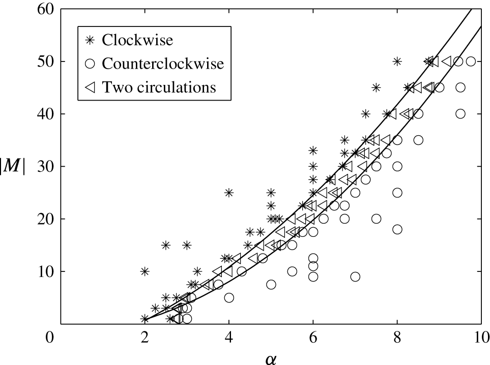
are plotted in figure 6.
Signs of the circulation in the first quadrant on the
 $\unicode[STIX]{x1D719}=0$
plane at different
 $|M|$
and
 $\unicode[STIX]{x1D6FC}$
values.

Corresponding to
 $|M|=10$
, the transition for flow reversal (figure 4
b,c) is approximately at
 $\unicode[STIX]{x1D6FC}=4$
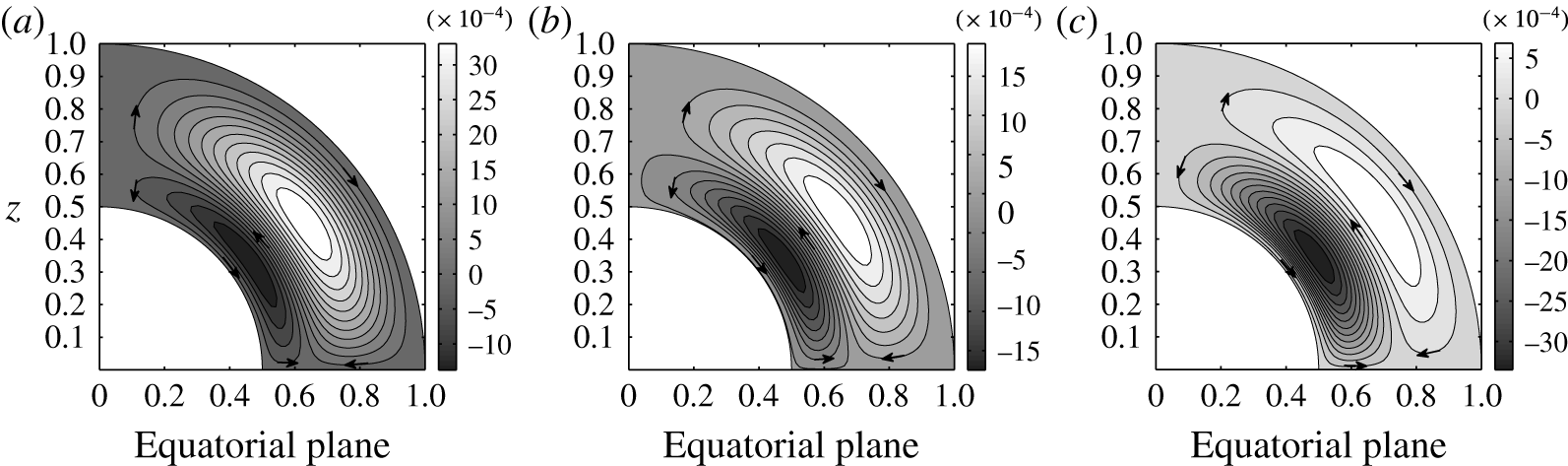
. The flow field around this transition is detailed in figure 7(a–c). Some interesting flow patterns have been predicted. With the increase of
 $\unicode[STIX]{x1D6FC}$
, a second vortex with opposite circulation is formed close to the inner boundary (figure 7
a) around
 $\unicode[STIX]{x1D6FC}=3.9$
. It then grows bigger with increasing
 $\unicode[STIX]{x1D6FC}$
and eventually squeezes out the existing clockwise-directed vortex in the first quadrant on the
 $\unicode[STIX]{x1D719}=0$
plane (figure 7
b,c).
Example of the streaming flow pattern change on
 $r$
–
 $\unicode[STIX]{x1D703}$
plane under different amplitude ratio (
 $|M|=10$
,
 $b=0.5$
). (a)
 $\unicode[STIX]{x1D6FC}=3.9$
, (b)
 $\unicode[STIX]{x1D6FC}=4.0$
, (c)
 $\unicode[STIX]{x1D6FC}=4.1$
.

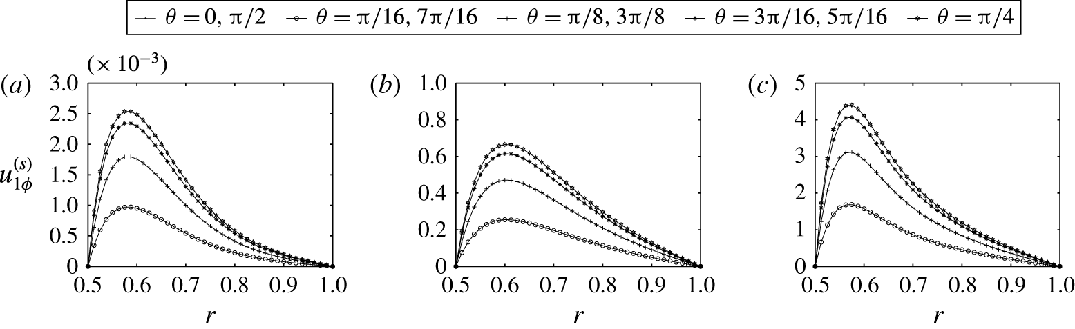
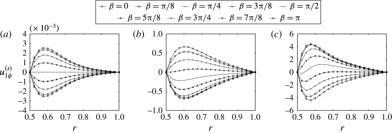
For the steady part of first-order azimuthal velocity
 $u_{1\unicode[STIX]{x1D719}}^{(s)}$
, the value is proportional to the oscillation amplitude ratio
 $\unicode[STIX]{x1D6FC}$
according to (2.20), (2.29) and (2.49). So increasing
 $\unicode[STIX]{x1D6FC}$
does not change the direction of the azimuthal velocity, but the value. When compared with the low frequency in figure 8, higher-frequency oscillations can induce more intense streaming. At low frequencies, the azimuthal velocity
 $u_{1\unicode[STIX]{x1D719}}^{(s)}$
is insignificant.
Steady part of first order azimuthal velocity profiles with
 $b=0.5$
,
 $\unicode[STIX]{x1D6FC}=1$
and
 $\unicode[STIX]{x1D6FD}=0$
. (a) low frequency, (b)
 $|M|=10$
, (c) high frequency
 $(|M|=25)$
.

The phase difference
 $\unicode[STIX]{x1D6FD}$
between the transverse and torsional oscillations does not have an influence on the leading-order solutions, nor on steady streaming on
 $r$
–
 $\unicode[STIX]{x1D703}$
plane either. However, to order
 $\unicode[STIX]{x1D700}$
, various values of the steady part of the azimuthal velocity are seen with variations of the phase difference
 $\unicode[STIX]{x1D6FD}$
, as shown in figure 9. The magnitude of
 $u_{1\unicode[STIX]{x1D719}}^{(s)}$
is the greatest for cases in which the phase difference
 $\unicode[STIX]{x1D6FD}$
is approximately
 $n\unicode[STIX]{x03C0}$
, where
 $n=0,1$
. For low-frequency oscillation, the azimuthal velocity
 $u_{1\unicode[STIX]{x1D719}}^{(s)}$
vanishes at a phase difference
 $\unicode[STIX]{x1D6FD}=((2n+1)\unicode[STIX]{x03C0})/2$
, and no recirculation appears on the
 $r$
–
 $\unicode[STIX]{x1D719}$
plane for any values of phase difference
 $\unicode[STIX]{x1D6FD}$
(figure 9
a). For higher frequency, take
 $|M|=10$
for example (figure 9
b), the azimuthal velocity
 $u_{1\unicode[STIX]{x1D719}}^{(s)}$
still exists at a phase difference
 $\unicode[STIX]{x1D6FD}=((2n+1)\unicode[STIX]{x03C0})/2$
. However, under high-frequency oscillations (figure 9
c), steady streaming has a recirculation on
 $r$
–
 $\unicode[STIX]{x1D719}$
plane when the phase difference
 $\unicode[STIX]{x1D6FD}$
is approximately in the range from
 $((2n+1)\unicode[STIX]{x03C0})/2$
to
 $((2n+1)\unicode[STIX]{x03C0}+1/4\unicode[STIX]{x03C0})/2$
.
Steady part of first-order azimuthal velocity profiles on the plane
 $\unicode[STIX]{x1D703}=\unicode[STIX]{x03C0}/4$
under different phase difference
 $\unicode[STIX]{x1D6FD}$
with
 $b=0.5$
,
 $\unicode[STIX]{x1D6FC}=1$
. (a) Low frequency, (b)
 $|M|=10$
, (c) high frequency
 $(|M|=25)$
.

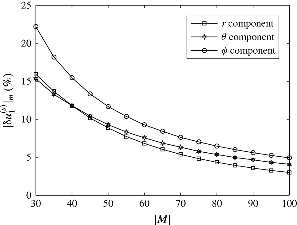
Since we have results for unrestricted
 $|M|$
in (2.20), we are in a position to compare these with asymptotic analysis for
 $|M|\gg 1$
. A comparison for various
 $|M|$
values has been made. Specifically, we have plotted the maximum relative error of the velocity components
 $u_{1r}^{(s)}$
,
 $u_{1\unicode[STIX]{x1D703}}^{(s)}$
,
 $u_{1\unicode[STIX]{x1D719}}^{(s)}$
between the asymptotic results and the unrestricted
 $|M|$
ones as a function of
 $r$
for various values of
 $\unicode[STIX]{x1D703}$
when
 $|M|$
is between 30 and 100 in figure 10. The plot corresponds to
 $\unicode[STIX]{x1D6FC}=1$
,
 $\unicode[STIX]{x1D6FD}=0$
and
 $b=0.5$
. The asymptotic results from (2.49) show good agreement with the unrestricted
 $|M|$
results from (2.20), particularly for
 $|M|=100$
.


4 Discussion
The present work is concerned with flow induced by combined torsional and transverse oscillations of the inner sphere with a phase lag and amplitude difference in a concentric spherical container. Mathematical analysis has been carried out to obtain the leading-order shear stress distribution and steady streaming characteristics for a large range of Womersley number. Steady streaming is especially discussed for low and high frequency (
 $|M|\ll 1$
and
 $|M|\gg 1$
).
The leading-order shear stresses
 $\unicode[STIX]{x1D70F}_{0r\unicode[STIX]{x1D719}}$
and
 $\unicode[STIX]{x1D70F}_{0r\unicode[STIX]{x1D703}}$
result from the torsional and transverse oscillations, respectively. These shear stresses
 $\unicode[STIX]{x1D70F}_{0r\unicode[STIX]{x1D719}}$
and
 $\unicode[STIX]{x1D70F}_{0r\unicode[STIX]{x1D703}}$
have a perfect agreement with those induced by single oscillations in our previous work (Kong et al.
Reference Kong, Penkova and Sadhal2015), which was for unrestricted
 $|M|$
values. The velocity field for steady streaming for the combined oscillations is fully three-dimensional. In particular, the combination produces the
 $\unicode[STIX]{x1D719}$
-component of
 $O(\unicode[STIX]{x1D700})$
streaming which is absent in the separate torsional and transverse oscillation cases. This is an effect of the nonlinearity of the combination. The amplitude ratio
 $\unicode[STIX]{x1D6FC}$
and phase difference
 $\unicode[STIX]{x1D6FD}$
of two oscillations are important in the determination of steady streaming. On the
 $r$
–
 $\unicode[STIX]{x1D703}$
plane, since the directions of streaming recirculation are opposite to the single torsional and transverse cases, there is a transition point where the recirculation changes direction when increasing the amplitude ratio
 $\unicode[STIX]{x1D6FC}$
. The
 $\unicode[STIX]{x1D6FC}$
value for the transition point goes up with an increase of Womersley number
 $|M|$
. At high frequency, the effects of transverse oscillation are more obvious compared to those of torsional oscillation. On the other hand, for the azimuthal velocity
 $u_{1\unicode[STIX]{x1D719}}^{(s)}$
of steady streaming, the amplitude ratio
 $\unicode[STIX]{x1D6FC}$
affects only the value. In addition, the effects of the phase difference
 $\unicode[STIX]{x1D6FD}$
on the azimuthal velocity
 $u_{1\unicode[STIX]{x1D719}}^{(s)}$
are also discussed. According to the momentum equation (2.5a
), the
 $r$
and
 $\unicode[STIX]{x1D703}$
components of the streaming velocity, represented by the streaming flow stream function
 $\unicode[STIX]{x1D713}_{10}$
, result from interaction of the leading-order stream function
 $\unicode[STIX]{x1D713}_{0}$
with itself, or the leading-order angular circulation
 $\unicode[STIX]{x1D6FA}_{0}$
with itself. The leading-order stream function
 $\unicode[STIX]{x1D713}_{0}$
comes only from transverse oscillation, while the leading-order angular circulation
 $\unicode[STIX]{x1D6FA}_{0}$
comes only from torsional oscillation. So the phase difference
 $\unicode[STIX]{x1D6FD}$
between the two oscillations does not affect streaming on the
 $r$
–
 $\unicode[STIX]{x1D703}$
plane. On the other hand, from the momentum equation (2.5b
), we see that the nonlinear term in the equation of angular circulation
 $\unicode[STIX]{x1D6FA}$
, reflecting velocity in the
 $\unicode[STIX]{x1D719}$
direction, is the interaction of the stream function
 $\unicode[STIX]{x1D713}$
and the angular circulation
 $\unicode[STIX]{x1D6FA}$
. Thus, the phase difference
 $\unicode[STIX]{x1D6FD}$
only has an influence on the
 $\unicode[STIX]{x1D719}$
component of the streaming velocity. When
 $\unicode[STIX]{x1D6FD}$
is in a small range around
 $((2n+1)\unicode[STIX]{x03C0})/2$
, steady streaming has a recirculation on the
 $r$
–
 $\unicode[STIX]{x1D719}$
plane under high-frequency oscillation, while no recirculation appears and
 $u_{1\unicode[STIX]{x1D719}}^{(s)}$
vanishes under low-frequency oscillation.
The important contribution here is the analysis of streaming flow within a spherical annulus driven by two oscillatory motions (transverse and torsional) of the inner sphere. As is well known in streaming studies, non-zero mean flow happens at lower orders of perturbation than the case of just one type of oscillation. This phenomenon was illustrated by Kelly (Reference Kelly1966) and in the context of the application to spherical geometry in the work of Longuet-Higgins (Reference Longuet-Higgins1998) pertaining to radial pulsation combined with transverse oscillations of a bubble. This problem concerns the exterior of the bubble and the axially symmetric streaming flow does not have a vortical structure. On the other hand, the work of Gopinath (Reference Gopinath1994) combines torsional and transverse oscillations of a solid sphere leading to fully three-dimensional streaming. Our work builds further on this, and the streaming flow within the annular space is analysed. With both rigid walls, a double boundary-layer structure is found. In addition, there is an interesting vortical structure within the annulus. The double vortical structure takes place in a narrow band on the
 $\unicode[STIX]{x1D6FC}$
–
 $|M|$
plane, where
 $\unicode[STIX]{x1D6FC}$
is the amplitude ratio between the two oscillations. Outside this band, there is a single vortex structure in each hemisphere.
Appendix A. Derivation of (2.49)
In the boundary layer around the inner sphere,
 $\unicode[STIX]{x1D6F9}_{1}$
and
 $\unicode[STIX]{x1D6FA}_{1}$
satisfy
 $$\begin{eqnarray}\displaystyle \frac{\unicode[STIX]{x2202}}{\unicode[STIX]{x2202}t}\left(\frac{\unicode[STIX]{x2202}^{2}\unicode[STIX]{x1D6F9}_{1}}{\unicode[STIX]{x2202}\unicode[STIX]{x1D702}^{2}}\right)-\frac{1}{2}\frac{\unicode[STIX]{x2202}^{4}\unicode[STIX]{x1D6F9}_{1}}{\unicode[STIX]{x2202}\unicode[STIX]{x1D702}^{4}} & = & \displaystyle -\frac{1}{b^{2}}\left[\frac{\unicode[STIX]{x2202}\displaystyle \left(\unicode[STIX]{x1D6F9}_{0},\frac{\unicode[STIX]{x2202}^{2}\unicode[STIX]{x1D6F9}_{0}}{\unicode[STIX]{x2202}\unicode[STIX]{x1D702}^{2}}\right)}{\unicode[STIX]{x2202}(\unicode[STIX]{x1D702},\unicode[STIX]{x1D707})}+2\frac{\unicode[STIX]{x1D707}}{(1-\unicode[STIX]{x1D707}^{2})}\frac{\unicode[STIX]{x2202}\unicode[STIX]{x1D6F9}_{0}}{\unicode[STIX]{x2202}\unicode[STIX]{x1D702}}\frac{\unicode[STIX]{x2202}^{2}\unicode[STIX]{x1D6F9}_{0}}{\unicode[STIX]{x2202}\unicode[STIX]{x1D702}^{2}}\right.\nonumber\\ \displaystyle & & \displaystyle \left.+\,2\frac{\unicode[STIX]{x1D707}}{(1-\unicode[STIX]{x1D707}^{2})}\unicode[STIX]{x1D6FA}_{0}\frac{\unicode[STIX]{x2202}\unicode[STIX]{x1D6FA}_{0}}{\unicode[STIX]{x2202}\unicode[STIX]{x1D702}}\vphantom{\frac{\unicode[STIX]{x2202}\displaystyle \left(\unicode[STIX]{x1D6F9}_{0},\frac{\unicode[STIX]{x2202}^{2}\unicode[STIX]{x1D6F9}_{0}}{\unicode[STIX]{x2202}\unicode[STIX]{x1D702}^{2}}\right)}{\unicode[STIX]{x2202}\unicode[STIX]{x1D702}}}\right],\end{eqnarray}$$
 $$\begin{eqnarray}\displaystyle \frac{\unicode[STIX]{x2202}\unicode[STIX]{x1D6FA}_{1}}{\unicode[STIX]{x2202}t}-\frac{1}{2}\frac{\unicode[STIX]{x2202}^{2}\unicode[STIX]{x1D6FA}_{1}}{\unicode[STIX]{x2202}\unicode[STIX]{x1D702}^{2}} & = & \displaystyle -\frac{1}{b^{2}}\frac{\unicode[STIX]{x2202}(\unicode[STIX]{x1D6F9}_{0},\unicode[STIX]{x1D6FA}_{0})}{\unicode[STIX]{x2202}(\unicode[STIX]{x1D702},\unicode[STIX]{x1D707})},\end{eqnarray}$$
 $$\begin{eqnarray}\frac{\unicode[STIX]{x2202}\unicode[STIX]{x1D6F9}_{1}}{\unicode[STIX]{x2202}\unicode[STIX]{x1D707}}=\frac{\unicode[STIX]{x2202}\unicode[STIX]{x1D6F9}_{1}}{\unicode[STIX]{x2202}\unicode[STIX]{x1D702}}=\unicode[STIX]{x1D6FA}_{1}=0\quad \text{on }\unicode[STIX]{x1D702}=0.\end{eqnarray}$$
The solutions of
 $\unicode[STIX]{x1D6F9}_{1}$
and
 $\unicode[STIX]{x1D6FA}_{1}$
are sought in the form
 $$\begin{eqnarray}\displaystyle \unicode[STIX]{x1D6F9}_{1} & = & \displaystyle \unicode[STIX]{x1D6F9}_{1}^{(s)}+\unicode[STIX]{x1D6F9}_{1}^{(u)}=\unicode[STIX]{x1D6F9}_{10}(\unicode[STIX]{x1D702})\unicode[STIX]{x1D707}(1-\unicode[STIX]{x1D707}^{2})+\{\unicode[STIX]{x1D6F9}_{12}(\unicode[STIX]{x1D702})\text{e}^{2\text{i}t}\unicode[STIX]{x1D707}(1-\unicode[STIX]{x1D707}^{2})+\text{c.c.}\},\end{eqnarray}$$
 $$\begin{eqnarray}\displaystyle \unicode[STIX]{x1D6FA}_{1} & = & \displaystyle \unicode[STIX]{x1D6FA}_{1}^{(s)}+\unicode[STIX]{x1D6FA}_{1}^{(u)}=\unicode[STIX]{x1D6FA}_{10}(\unicode[STIX]{x1D702})\unicode[STIX]{x1D707}(1-\unicode[STIX]{x1D707}^{2})+\{\unicode[STIX]{x1D6FA}_{12}(\unicode[STIX]{x1D702})\text{e}^{2\text{i}t}\unicode[STIX]{x1D707}(1-\unicode[STIX]{x1D707}^{2})+\text{c.c.}\}.\end{eqnarray}$$
 $$\begin{eqnarray}\displaystyle \unicode[STIX]{x1D6F9}_{1}^{(s)} & = & \displaystyle \left\{\frac{2}{b^{2}}\left[\frac{1+\text{i}}{32}\left(\frac{9}{4}\left(\frac{b}{1-b^{3}}\right)^{2}-(\unicode[STIX]{x1D6FC}b)^{2}\right)\text{e}^{-2\unicode[STIX]{x1D702}}-\frac{3}{4}\left(\frac{\text{i}}{4}\frac{|M|}{\sqrt{2}}b^{2}+(1+\text{i})b\right.\right.\right.\nonumber\\ \displaystyle & & \displaystyle \left.-\,\frac{3(5+3\text{i})}{8}\left(\frac{b}{1-b^{3}}\right)\right)\frac{b}{1-b^{3}}\text{e}^{-(1+\text{i})\unicode[STIX]{x1D702}}\nonumber\\ \displaystyle & & \displaystyle \left.-\,\frac{3\text{i}}{8}\left(b-\frac{3}{2}\left(\frac{b}{1-b^{3}}\right)\right)\frac{b}{1-b^{3}}\unicode[STIX]{x1D702}\text{e}^{-(1+\text{i})\unicode[STIX]{x1D702}}\right]\nonumber\\ \displaystyle & & \displaystyle \left.+\,A_{1}\unicode[STIX]{x1D702}^{3}+B_{1}\unicode[STIX]{x1D702}^{2}+C_{1}\unicode[STIX]{x1D702}+D_{1}\right\}\unicode[STIX]{x1D707}(1-\unicode[STIX]{x1D707}^{2})+\text{c.c.},\end{eqnarray}$$
 $$\begin{eqnarray}\displaystyle \unicode[STIX]{x1D6FA}_{1}^{(s)} & = & \displaystyle \left\{\frac{2\unicode[STIX]{x1D6FC}\text{e}^{\text{i}\unicode[STIX]{x1D6FD}}}{b}\left[-\frac{3(1-\text{i})}{16}\frac{b}{1-b^{3}}\text{e}^{-2\unicode[STIX]{x1D702}}+\frac{1}{4}\left(-\frac{(1-\text{i})}{2}\frac{|M|}{\sqrt{2}}b^{2}+3\text{i}b\right.\right.\right.\nonumber\\ \displaystyle & & \displaystyle \left.\left.-\,\frac{3(1+3\text{i})}{2}\left(\frac{b}{1-b^{3}}\right)\right)\text{e}^{-(1+\text{i})\unicode[STIX]{x1D702}}-\frac{1-\text{i}}{4}\left(b-\frac{3}{2}\left(\frac{b}{1-b^{3}}\right)\right)\unicode[STIX]{x1D702}\text{e}^{-(1+\text{i})\unicode[STIX]{x1D702}}\right]\nonumber\\ \displaystyle & & \displaystyle \left.+\,A_{1}^{\ast }\unicode[STIX]{x1D702}+B_{1}^{\ast }\right\}\unicode[STIX]{x1D707}(1-\unicode[STIX]{x1D707}^{2})+\text{c.c.}\end{eqnarray}$$
In the boundary layer on the container, we have
 $$\begin{eqnarray}\displaystyle \frac{\unicode[STIX]{x2202}}{\unicode[STIX]{x2202}t}\left(\frac{\unicode[STIX]{x2202}^{2}\bar{\unicode[STIX]{x1D6F9}}_{1}}{\unicode[STIX]{x2202}\hat{\unicode[STIX]{x1D702}}^{2}}\right)-\frac{1}{2}\frac{\unicode[STIX]{x2202}^{4}\bar{\unicode[STIX]{x1D6F9}}_{1}}{\unicode[STIX]{x2202}\hat{\unicode[STIX]{x1D702}}^{4}} & = & \displaystyle \frac{\unicode[STIX]{x2202}\displaystyle \left(\bar{\unicode[STIX]{x1D6F9}}_{0},\frac{\unicode[STIX]{x2202}^{2}\bar{\unicode[STIX]{x1D6F9}}_{0}}{\unicode[STIX]{x2202}\hat{\unicode[STIX]{x1D702}}^{2}}\right)}{\unicode[STIX]{x2202}(\hat{\unicode[STIX]{x1D702}},\unicode[STIX]{x1D707})}+2\frac{\unicode[STIX]{x1D707}}{(1-\unicode[STIX]{x1D707}^{2})}\frac{\unicode[STIX]{x2202}\bar{\unicode[STIX]{x1D6F9}}_{0}}{\unicode[STIX]{x2202}\hat{\unicode[STIX]{x1D702}}}\frac{\unicode[STIX]{x2202}^{2}\bar{\unicode[STIX]{x1D6F9}}_{0}}{\unicode[STIX]{x2202}\hat{\unicode[STIX]{x1D702}}^{2}}\nonumber\\ \displaystyle & & \displaystyle +\,2\frac{\unicode[STIX]{x1D707}}{(1-\unicode[STIX]{x1D707}^{2})}\unicode[STIX]{x1D6FA}_{0}\frac{\unicode[STIX]{x2202}\unicode[STIX]{x1D6FA}_{0}}{\unicode[STIX]{x2202}\hat{\unicode[STIX]{x1D702}}},\end{eqnarray}$$
 $$\begin{eqnarray}\displaystyle \frac{\unicode[STIX]{x2202}\unicode[STIX]{x1D6FA}_{1}}{\unicode[STIX]{x2202}t}-\frac{1}{2}\frac{\unicode[STIX]{x2202}^{2}\unicode[STIX]{x1D6FA}_{1}}{\unicode[STIX]{x2202}\hat{\unicode[STIX]{x1D702}}^{2}} & = & \displaystyle \frac{\unicode[STIX]{x2202}(\bar{\unicode[STIX]{x1D6F9}}_{0},\unicode[STIX]{x1D6FA}_{0})}{\unicode[STIX]{x2202}(\hat{\unicode[STIX]{x1D702}},\unicode[STIX]{x1D707})},\end{eqnarray}$$
 $$\begin{eqnarray}\frac{\unicode[STIX]{x2202}\bar{\unicode[STIX]{x1D6F9}}_{1}}{\unicode[STIX]{x2202}\unicode[STIX]{x1D707}}=\frac{\unicode[STIX]{x2202}\bar{\unicode[STIX]{x1D6F9}}_{1}}{\unicode[STIX]{x2202}\hat{\unicode[STIX]{x1D702}}}=\unicode[STIX]{x1D6FA}_{1}=0\quad \text{on }\hat{\unicode[STIX]{x1D702}}=0.\end{eqnarray}$$
Similarly, we write
 $\bar{\unicode[STIX]{x1D6F9}}_{1}$
and
 $\unicode[STIX]{x1D6FA}_{1}$
as
 $$\begin{eqnarray}\displaystyle \bar{\unicode[STIX]{x1D6F9}}_{1} & = & \displaystyle \bar{\unicode[STIX]{x1D6F9}}_{1}^{(s)}+\bar{\unicode[STIX]{x1D6F9}}_{1}^{(u)}=\bar{\unicode[STIX]{x1D6F9}}_{10}(\hat{\unicode[STIX]{x1D702}})\unicode[STIX]{x1D707}(1-\unicode[STIX]{x1D707}^{2})+\{\bar{\unicode[STIX]{x1D6F9}}_{12}(\hat{\unicode[STIX]{x1D702}})\text{e}^{2\text{i}t}\unicode[STIX]{x1D707}(1-\unicode[STIX]{x1D707}^{2})+\text{c.c.}\},\end{eqnarray}$$
 $$\begin{eqnarray}\displaystyle \unicode[STIX]{x1D6FA}_{1} & = & \displaystyle \unicode[STIX]{x1D6FA}_{1}^{(s)}+\unicode[STIX]{x1D6FA}_{1}^{(u)}=\unicode[STIX]{x1D6FA}_{10}(\hat{\unicode[STIX]{x1D702}})\unicode[STIX]{x1D707}(1-\unicode[STIX]{x1D707}^{2})+\{\unicode[STIX]{x1D6FA}_{12}(\hat{\unicode[STIX]{x1D702}})\text{e}^{2\text{i}t}\unicode[STIX]{x1D707}(1-\unicode[STIX]{x1D707}^{2})+\text{c.c.}\}.\end{eqnarray}$$
 $$\begin{eqnarray}\displaystyle \bar{\unicode[STIX]{x1D6F9}}_{1}^{(s)} & = & \displaystyle \left\{-\frac{9}{8}\frac{b^{6}}{(1-b^{3})^{2}}\left[\frac{1+\text{i}}{8}\text{e}^{-2\hat{\unicode[STIX]{x1D702}}}+\frac{5+3\text{i}}{2}\text{e}^{-(1+\text{i})\hat{\unicode[STIX]{x1D702}}}+\text{i}\hat{\unicode[STIX]{x1D702}}\text{e}^{-(1+\text{i})\hat{\unicode[STIX]{x1D702}}}\right]\right.\nonumber\\ \displaystyle & & \displaystyle \left.+\,A_{2}\hat{\unicode[STIX]{x1D702}}^{3}+B_{2}\hat{\unicode[STIX]{x1D702}}^{2}+C_{2}\hat{\unicode[STIX]{x1D702}}+D_{2}\right\}\unicode[STIX]{x1D707}(1-\unicode[STIX]{x1D707}^{2})+\text{c.c.},\end{eqnarray}$$
 $$\begin{eqnarray}\displaystyle \unicode[STIX]{x1D6FA}_{1}^{(s)} & = & \displaystyle A_{2}^{\ast }\hat{\unicode[STIX]{x1D702}}\unicode[STIX]{x1D707}(1-\unicode[STIX]{x1D707}^{2})+\text{c.c.}\end{eqnarray}$$
All the coefficients need to be determined by boundary conditions and matching with the outer flow.
Accordingly, in the outer region, only
 $R_{s}\ll 1$
is considered. We write
 $$\begin{eqnarray}\displaystyle & \displaystyle \unicode[STIX]{x1D713}=\unicode[STIX]{x1D713}_{0}+\unicode[STIX]{x1D700}\unicode[STIX]{x1D709}+O(\unicode[STIX]{x1D700}^{2}), & \displaystyle\end{eqnarray}$$
 $$\begin{eqnarray}\displaystyle & \displaystyle \unicode[STIX]{x1D6FA}=\unicode[STIX]{x1D6FA}_{0}+\unicode[STIX]{x1D700}\unicode[STIX]{x1D701}+O(\unicode[STIX]{x1D700}^{2}), & \displaystyle\end{eqnarray}$$
 $\unicode[STIX]{x1D713}_{0}$
and
 $\unicode[STIX]{x1D6FA}_{0}$
are given before, and
 $\unicode[STIX]{x1D709}$
and
 $\unicode[STIX]{x1D701}$
satisfy
 $$\begin{eqnarray}\displaystyle & & \displaystyle R_{s}\frac{\unicode[STIX]{x2202}}{\unicode[STIX]{x2202}t}(\text{D}^{2}\unicode[STIX]{x1D709})+\frac{\unicode[STIX]{x1D700}R_{s}}{r^{2}}\left[\frac{\unicode[STIX]{x2202}}{\unicode[STIX]{x2202}r}(\unicode[STIX]{x1D713}_{0}+\unicode[STIX]{x1D700}\unicode[STIX]{x1D709})\frac{\unicode[STIX]{x2202}}{\unicode[STIX]{x2202}\unicode[STIX]{x1D707}}(\text{D}^{2}\unicode[STIX]{x1D709})-\frac{\unicode[STIX]{x2202}}{\unicode[STIX]{x2202}\unicode[STIX]{x1D707}}(\unicode[STIX]{x1D713}_{0}+\unicode[STIX]{x1D700}\unicode[STIX]{x1D709})\frac{\unicode[STIX]{x2202}}{\unicode[STIX]{x2202}r}(\text{D}^{2}\unicode[STIX]{x1D709})\right.\nonumber\\ \displaystyle & & \displaystyle \quad \left.+\,2\text{D}^{2}\unicode[STIX]{x1D709}\text{L}(\unicode[STIX]{x1D713}_{0}+\unicode[STIX]{x1D700}\unicode[STIX]{x1D709})+2\unicode[STIX]{x1D700}\unicode[STIX]{x1D701}\text{L}\unicode[STIX]{x1D701}\right]=\unicode[STIX]{x1D700}^{2}\text{D}^{4}\unicode[STIX]{x1D709},\end{eqnarray}$$
 $$\begin{eqnarray}\displaystyle & & \displaystyle R_{s}\frac{\unicode[STIX]{x2202}\unicode[STIX]{x1D701}}{\unicode[STIX]{x2202}t}+\frac{\unicode[STIX]{x1D700}R_{s}}{r^{2}}\left[\frac{\unicode[STIX]{x2202}}{\unicode[STIX]{x2202}r}(\unicode[STIX]{x1D713}_{0}+\unicode[STIX]{x1D700}\unicode[STIX]{x1D709})\frac{\unicode[STIX]{x2202}\unicode[STIX]{x1D701}}{\unicode[STIX]{x2202}\unicode[STIX]{x1D707}}-\frac{\unicode[STIX]{x2202}}{\unicode[STIX]{x2202}\unicode[STIX]{x1D707}}(\unicode[STIX]{x1D713}_{0}+\unicode[STIX]{x1D700}\unicode[STIX]{x1D709})\frac{\unicode[STIX]{x2202}\unicode[STIX]{x1D701}}{\unicode[STIX]{x2202}r}\right]=\unicode[STIX]{x1D700}^{2}\text{D}^{2}\unicode[STIX]{x1D701},\end{eqnarray}$$
 $\text{L}$
is defined in (2.7).
We now expand
 $\unicode[STIX]{x1D709}(r,\unicode[STIX]{x1D707},t,\unicode[STIX]{x1D700})$
and
 $\unicode[STIX]{x1D701}(r,\unicode[STIX]{x1D707},t,\unicode[STIX]{x1D700})$
in the form
 $$\begin{eqnarray}\displaystyle \unicode[STIX]{x1D709} & = & \displaystyle \unicode[STIX]{x1D709}_{1}+\unicode[STIX]{x1D700}\unicode[STIX]{x1D709}_{2}+\cdots \,,\end{eqnarray}$$
 $$\begin{eqnarray}\displaystyle \unicode[STIX]{x1D701} & = & \displaystyle \unicode[STIX]{x1D701}_{1}+\unicode[STIX]{x1D700}\unicode[STIX]{x1D701}_{2}+\cdots \,.\end{eqnarray}$$
 $O(1)$
in (A 9) require that
 $\unicode[STIX]{x1D709}_{1}$
and
 $\unicode[STIX]{x1D701}_{1}$
satisfy
 $$\begin{eqnarray}\frac{\unicode[STIX]{x2202}}{\unicode[STIX]{x2202}t}(\text{D}^{2}\unicode[STIX]{x1D709}_{1})=0\quad \text{and}\quad \frac{\unicode[STIX]{x2202}\unicode[STIX]{x1D701}_{1}}{\unicode[STIX]{x2202}t}=0,\end{eqnarray}$$
the solutions of which are
 $$\begin{eqnarray}\unicode[STIX]{x1D709}_{1}=F_{10}(r,\unicode[STIX]{x1D707})+F_{12}(r,\unicode[STIX]{x1D707})\tilde{T}_{1}(t)+\text{c.c.}\quad \text{and}\quad \unicode[STIX]{x1D701}_{1}=G_{10}(r,\unicode[STIX]{x1D707})+\text{c.c.},\end{eqnarray}$$
with
 $$\begin{eqnarray}\text{D}^{2}F_{12}(r,\unicode[STIX]{x1D707})=0.\end{eqnarray}$$
The terms of
 $O(\unicode[STIX]{x1D700})$
give the equation for
 $\unicode[STIX]{x1D709}_{2}$
and
 $\unicode[STIX]{x1D701}_{2}$
as
 $$\begin{eqnarray}\displaystyle & \displaystyle \frac{\unicode[STIX]{x2202}}{\unicode[STIX]{x2202}t}(\text{D}^{2}\unicode[STIX]{x1D709}_{2})+\frac{1}{r^{2}}\left[\frac{\unicode[STIX]{x2202}\unicode[STIX]{x1D713}_{0}}{\unicode[STIX]{x2202}r}\frac{\unicode[STIX]{x2202}}{\unicode[STIX]{x2202}\unicode[STIX]{x1D707}}(\text{D}^{2}\unicode[STIX]{x1D709}_{1})-\frac{\unicode[STIX]{x2202}\unicode[STIX]{x1D713}_{0}}{\unicode[STIX]{x2202}\unicode[STIX]{x1D707}}\frac{\unicode[STIX]{x2202}}{\unicode[STIX]{x2202}r}(\text{D}^{2}\unicode[STIX]{x1D709}_{1})+2\text{D}^{2}\unicode[STIX]{x1D709}_{1}\text{L}\unicode[STIX]{x1D713}_{0}\right]=0, & \displaystyle\end{eqnarray}$$
 $$\begin{eqnarray}\displaystyle & \displaystyle \frac{\unicode[STIX]{x2202}\unicode[STIX]{x1D701}_{2}}{\unicode[STIX]{x2202}t}+\frac{1}{r^{2}}\left[\frac{\unicode[STIX]{x2202}\unicode[STIX]{x1D713}_{0}}{\unicode[STIX]{x2202}r}\frac{\unicode[STIX]{x2202}\unicode[STIX]{x1D701}_{1}}{\unicode[STIX]{x2202}\unicode[STIX]{x1D707}}-\frac{\unicode[STIX]{x2202}\unicode[STIX]{x1D713}_{0}}{\unicode[STIX]{x2202}\unicode[STIX]{x1D707}}\frac{\unicode[STIX]{x2202}\unicode[STIX]{x1D701}_{1}}{\unicode[STIX]{x2202}r}\right]=0, & \displaystyle\end{eqnarray}$$
 $$\begin{eqnarray}\unicode[STIX]{x1D709}_{2}=F_{20}(r,\unicode[STIX]{x1D707})+F_{22}(r,\unicode[STIX]{x1D707})\tilde{T}_{2}(t)+\text{c.c.}\quad \text{and}\quad \unicode[STIX]{x1D701}_{2}=G_{20}(r,\unicode[STIX]{x1D707})+G_{22}(r,\unicode[STIX]{x1D707})\tilde{T}_{2}^{\ast }(t)+\text{c.c.}\end{eqnarray}$$
Since in (A 15),
 $\text{D}^{2}\unicode[STIX]{x1D709}_{1}$
is independent of
 $t$
from (A 12), and
 $\unicode[STIX]{x1D713}_{0}\propto \text{e}^{\text{i}t}$
from (2.43), we can write
 $\unicode[STIX]{x1D709}_{2}$
in the form
 $$\begin{eqnarray}\unicode[STIX]{x1D709}_{2}=F_{20}(r,\unicode[STIX]{x1D707})+F_{22}(r,\unicode[STIX]{x1D707})\text{e}^{\text{i}t}+\text{c.c.}\end{eqnarray}$$
Similarly, for
 $\unicode[STIX]{x1D701}_{2}$
, we have
 $$\begin{eqnarray}\unicode[STIX]{x1D701}_{2}=G_{20}(r,\unicode[STIX]{x1D707})+G_{22}(r,\unicode[STIX]{x1D707})\text{e}^{\text{i}t}+\text{c.c.}\end{eqnarray}$$
Then the equations for
 $\unicode[STIX]{x1D709}_{3}$
and
 $\unicode[STIX]{x1D701}_{3}$
, obtained from the
 $O(\unicode[STIX]{x1D700}^{2})$
terms are
 $$\begin{eqnarray}\displaystyle & & \displaystyle R_{s}\frac{\unicode[STIX]{x2202}}{\unicode[STIX]{x2202}t}(\text{D}^{2}\unicode[STIX]{x1D709}_{3})+\frac{R_{s}}{r^{2}}\left[\frac{\unicode[STIX]{x2202}\unicode[STIX]{x1D713}_{0}}{\unicode[STIX]{x2202}r}\frac{\unicode[STIX]{x2202}}{\unicode[STIX]{x2202}\unicode[STIX]{x1D707}}(\text{D}^{2}\unicode[STIX]{x1D709}_{2})-\frac{\unicode[STIX]{x2202}\unicode[STIX]{x1D713}_{0}}{\unicode[STIX]{x2202}\unicode[STIX]{x1D707}}\frac{\unicode[STIX]{x2202}}{\unicode[STIX]{x2202}r}(\text{D}^{2}\unicode[STIX]{x1D709}_{2})+2\text{D}^{2}\unicode[STIX]{x1D709}_{2}\text{L}\unicode[STIX]{x1D713}_{0}\right]\nonumber\\ \displaystyle & & \displaystyle \quad +\,\frac{R_{s}}{r^{2}}\left[\frac{\unicode[STIX]{x2202}\unicode[STIX]{x1D709}_{1}}{\unicode[STIX]{x2202}r}\frac{\unicode[STIX]{x2202}}{\unicode[STIX]{x2202}\unicode[STIX]{x1D707}}(\text{D}^{2}\unicode[STIX]{x1D709}_{1})-\frac{\unicode[STIX]{x2202}\unicode[STIX]{x1D709}_{1}}{\unicode[STIX]{x2202}\unicode[STIX]{x1D707}}\frac{\unicode[STIX]{x2202}}{\unicode[STIX]{x2202}r}(\text{D}^{2}\unicode[STIX]{x1D709}_{1})+2\text{D}^{2}\unicode[STIX]{x1D709}_{1}\text{L}\unicode[STIX]{x1D709}_{1}+2\unicode[STIX]{x1D701}_{1}\text{L}\unicode[STIX]{x1D701}_{1}\right]=\text{D}^{4}\unicode[STIX]{x1D709}_{1},\hspace{24.0pt}\end{eqnarray}$$
 $$\begin{eqnarray}\displaystyle & & \displaystyle R_{s}\frac{\unicode[STIX]{x2202}\unicode[STIX]{x1D701}_{3}}{\unicode[STIX]{x2202}t}+\frac{R_{s}}{r^{2}}\left[\frac{\unicode[STIX]{x2202}\unicode[STIX]{x1D713}_{0}}{\unicode[STIX]{x2202}r}\frac{\unicode[STIX]{x2202}\unicode[STIX]{x1D701}_{2}}{\unicode[STIX]{x2202}\unicode[STIX]{x1D707}}-\frac{\unicode[STIX]{x2202}\unicode[STIX]{x1D713}_{0}}{\unicode[STIX]{x2202}\unicode[STIX]{x1D707}}\frac{\unicode[STIX]{x2202}\unicode[STIX]{x1D701}_{2}}{\unicode[STIX]{x2202}r}\right]+\frac{R_{s}}{r^{2}}\left[\frac{\unicode[STIX]{x2202}\unicode[STIX]{x1D709}_{1}}{\unicode[STIX]{x2202}r}\frac{\unicode[STIX]{x2202}\unicode[STIX]{x1D701}_{1}}{\unicode[STIX]{x2202}\unicode[STIX]{x1D707}}-\frac{\unicode[STIX]{x2202}\unicode[STIX]{x1D709}_{1}}{\unicode[STIX]{x2202}\unicode[STIX]{x1D707}}\frac{\unicode[STIX]{x2202}\unicode[STIX]{x1D701}_{1}}{\unicode[STIX]{x2202}r}\right]=\text{D}^{2}\unicode[STIX]{x1D701}_{1}.\end{eqnarray}$$
 $(\unicode[STIX]{x2202}/\unicode[STIX]{x2202}t)(D^{2}\unicode[STIX]{x1D709}_{3})$
contains no steady part. Otherwise,
 $\unicode[STIX]{x1D709}_{3}$
would contain terms of
 $O(t)$
, which would lead to unbounded growth in time, according to Rosenblat (Reference Rosenblat1959). It is similar for
 $\unicode[STIX]{x2202}\unicode[STIX]{x1D701}_{3}/\unicode[STIX]{x2202}t$
.
Because the second terms of (A 19) are in proportion to
 $\sin t\cos t$
, they have no steady part. We may equate the time-independent parts of the
 $O(\unicode[STIX]{x1D700}^{2})$
equations, to get for the steady part
 $$\begin{eqnarray}\displaystyle & \displaystyle \frac{R_{s}}{r^{2}}\left[\frac{\unicode[STIX]{x2202}F_{10}}{\unicode[STIX]{x2202}r}\frac{\unicode[STIX]{x2202}}{\unicode[STIX]{x2202}\unicode[STIX]{x1D707}}(\text{D}^{2}F_{10})-\frac{\unicode[STIX]{x2202}F_{10}}{\unicode[STIX]{x2202}\unicode[STIX]{x1D707}}\frac{\unicode[STIX]{x2202}}{\unicode[STIX]{x2202}r}(\text{D}^{2}F_{10})+2\text{D}^{2}F_{10}\text{L}F_{10}+2G_{10}\text{L}G_{10}\right]=\text{D}^{4}F_{10},\hspace{30.0pt} & \displaystyle\end{eqnarray}$$
 $$\begin{eqnarray}\displaystyle & \displaystyle \frac{R_{s}}{r^{2}}\left[\frac{\unicode[STIX]{x2202}F_{10}}{\unicode[STIX]{x2202}r}\frac{\unicode[STIX]{x2202}G_{10}}{\unicode[STIX]{x2202}\unicode[STIX]{x1D707}}-\frac{\unicode[STIX]{x2202}F_{10}}{\unicode[STIX]{x2202}\unicode[STIX]{x1D707}}\frac{\unicode[STIX]{x2202}G_{10}}{\unicode[STIX]{x2202}r}\right]=\text{D}^{2}G_{10}. & \displaystyle\end{eqnarray}$$
 $R_{s}\ll 1$
in (A 19) resulting in Stokes-like steady flow, i.e.
 $$\begin{eqnarray}\text{D}^{4}F_{10}=0\quad \text{and}\quad \text{D}^{2}G_{10}=0.\end{eqnarray}$$
The appropriate form of solutions should be
 $$\begin{eqnarray}\displaystyle & \displaystyle F_{10}(r,\unicode[STIX]{x1D707})=\left(A_{3}r^{5}+B_{3}r^{3}+C_{3}+\frac{D_{3}}{r^{2}}\right)\unicode[STIX]{x1D707}(1-\unicode[STIX]{x1D707}^{2}), & \displaystyle\end{eqnarray}$$
 $$\begin{eqnarray}\displaystyle & \displaystyle G_{10}(r,\unicode[STIX]{x1D707})=\left(A_{3}^{\ast }r^{3}+\frac{B_{3}^{\ast }}{r^{2}}\right)\unicode[STIX]{x1D707}(1-\unicode[STIX]{x1D707}^{2}). & \displaystyle\end{eqnarray}$$
 $$\begin{eqnarray}\displaystyle \unicode[STIX]{x1D709}_{1}^{(s)} & = & \displaystyle \left(A_{3}r^{5}+B_{3}r^{3}+C_{3}+\frac{D_{3}}{r^{2}}\right)\unicode[STIX]{x1D707}(1-\unicode[STIX]{x1D707}^{2})+\text{c.c.},\end{eqnarray}$$
 $$\begin{eqnarray}\displaystyle \unicode[STIX]{x1D701}_{1}^{(s)} & = & \displaystyle \left(A_{3}^{\ast }r^{3}+\frac{B_{3}^{\ast }}{r^{2}}\right)\unicode[STIX]{x1D707}(1-\unicode[STIX]{x1D707}^{2})+\text{c.c.}\end{eqnarray}$$
Appendix B. Coefficients in (2.10), (2.20), (2.29) and (2.49)
Values of the coefficients are provided in this section. The coefficients in (2.10) are given by
 $$\begin{eqnarray}\displaystyle EA_{0} & = & \displaystyle -\frac{1}{4\text{i}}[\text{e}^{M(1-b)}(3+3Mb+M^{2}b^{2})-\text{e}^{M(b-1)}(3-3Mb+M^{2}b^{2})-6M],\hspace{24.0pt}\end{eqnarray}$$
 $$\begin{eqnarray}\displaystyle EB_{0} & = & \displaystyle \frac{1}{4\text{i}}\left[\text{e}^{M(1-b)}\left(\frac{3}{M}+3b+Mb^{2}\right)\left(\frac{3}{M}-3+M\right)\right.\nonumber\\ \displaystyle & & \displaystyle \left.-\,\text{e}^{M(b-1)}\left(\frac{3}{M}-3b+Mb^{2}\right)\left(\frac{3}{M}+3+M\right)\right],\end{eqnarray}$$
 $$\begin{eqnarray}\displaystyle EC_{0} & = & \displaystyle -\frac{1}{4\text{i}}\left[\text{e}^{-Mb}\left(\frac{9}{M}+9b+3Mb^{2}\right)-\text{e}^{-M}\left(\frac{9}{M}+9+3M\right)\right],\end{eqnarray}$$
 $$\begin{eqnarray}\displaystyle ED_{0} & = & \displaystyle \frac{1}{4\text{i}}\left[\text{e}^{Mb}\left(\frac{9}{M}-9b+3Mb^{2}\right)-\text{e}^{M}\left(\frac{9}{M}-9+3M\right)\right],\end{eqnarray}$$
 $$\begin{eqnarray}\displaystyle E & = & \displaystyle 12M+\text{e}^{M(1-b)}\left[3\left(\frac{1}{b}-1\right)-3M\left(\frac{1}{b}+b\right)+M^{2}\left(\frac{1}{b}-b^{2}\right)\right]\nonumber\\ \displaystyle & & \displaystyle -\,\text{e}^{M(b-1)}\left[3\left(\frac{1}{b}-1\right)+3M\left(\frac{1}{b}+b\right)+M^{2}\left(\frac{1}{b}-b^{2}\right)\right],\end{eqnarray}$$
 $$\begin{eqnarray}\displaystyle E^{\ast }A_{0}^{\ast } & = & \displaystyle -\frac{1}{2\text{i}}\unicode[STIX]{x1D6FC}\text{e}^{\text{i}\unicode[STIX]{x1D6FD}}\text{e}^{-M}\left(\frac{1}{M}+1\right),\end{eqnarray}$$
 $$\begin{eqnarray}\displaystyle E^{\ast }B_{0}^{\ast } & = & \displaystyle \frac{1}{2\text{i}}\unicode[STIX]{x1D6FC}\text{e}^{\text{i}\unicode[STIX]{x1D6FD}}\text{e}^{M}\left(\frac{1}{M}-1\right),\end{eqnarray}$$
 $$\begin{eqnarray}\displaystyle E^{\ast } & = & \displaystyle \left(\frac{1}{M}-1\right)\left(\frac{1}{Mb^{2}}+\frac{1}{b}\right)\text{e}^{M(1-b)}-\left(\frac{1}{M}+1\right)\left(\frac{1}{Mb^{2}}-\frac{1}{b}\right)\text{e}^{M(b-1)}.\end{eqnarray}$$
 $$\begin{eqnarray}\displaystyle c_{1}D^{\ast } & = & \displaystyle H_{1}(b)(-21b^{2}+25b^{4}-4b^{7})+H_{2}(b)(-15+15b^{2})+H_{3}(b)\left(-\frac{6}{b^{3}}+6b^{2}\right)\nonumber\\ \displaystyle & & \displaystyle +\,H_{4}(b)\left(-\frac{10}{b^{3}}+10\right)+H_{1}(1)\left(-\frac{4}{b^{3}}+25-21b^{2}\right)+H_{2}(1)(15-15b^{2})\nonumber\\ \displaystyle & & \displaystyle +\,H_{3}(1)\left(\frac{6}{b^{3}}-6b^{2}\right)+H_{4}(1)\left(\frac{10}{b^{3}}-10\right),\end{eqnarray}$$
 $$\begin{eqnarray}\displaystyle c_{2}D^{\ast } & = & \displaystyle H_{1}(b)(35b^{2}-35b^{4})+H_{2}(b)(25-21b^{2}-4b^{7})+H_{3}(b)\left(\frac{10}{b^{3}}-10b^{4}\right)\nonumber\\ \displaystyle & & \displaystyle +\,H_{4}(b)\left(\frac{14}{b^{3}}-14b^{2}\right)+H_{1}(1)(-35b^{2}+35b^{4})\nonumber\\ \displaystyle & & \displaystyle +\,H_{2}(1)\left(-\frac{4}{b^{3}}-21b^{2}+25b^{4}\right)+H_{3}(1)\left(-\frac{10}{b^{3}}+10b^{4}\right)\nonumber\\ \displaystyle & & \displaystyle +\,H_{4}(1)\left(-\frac{14}{b^{3}}+14b^{2}\right),\end{eqnarray}$$
 $$\begin{eqnarray}\displaystyle c_{3}D^{\ast } & = & \displaystyle H_{1}(b)(-14b^{2}+14b^{7})+H_{2}(b)(-10+10b^{7})+H_{3}(b)\left(-\frac{4}{b^{3}}-21b^{2}+25b^{4}\right)\nonumber\\ \displaystyle & & \displaystyle +\,H_{4}(b)(-35+35b^{2})+H_{1}(1)(14b^{2}-14b^{7})+H_{2}(1)(10-10b^{7})\nonumber\\ \displaystyle & & \displaystyle +\,H_{3}(1)(25-21b^{2}-4b^{7})+H_{4}(1)(35-35b^{2}),\end{eqnarray}$$
 $$\begin{eqnarray}\displaystyle c_{4}D^{\ast } & = & \displaystyle H_{1}(b)(10b^{4}-10b^{7})+H_{2}(b)(6b^{2}-6b^{7})+H_{3}(b)(15b^{2}-15b^{4})\nonumber\\ \displaystyle & & \displaystyle +\,H_{4}(b)\left(-\frac{4}{b^{3}}+25-21b^{2}\right)+H_{1}(1)(-10b^{4}+10b^{7})+H_{2}(1)(-6b^{2}+6b^{7})\nonumber\\ \displaystyle & & \displaystyle +\,H_{3}(1)(-15b^{2}+15b^{4})+H_{4}(1)(-21b^{2}+25b^{4}-4b^{7}),\end{eqnarray}$$
 $$\begin{eqnarray}\displaystyle c_{5} & = & \displaystyle \frac{1}{1-b^{5}}[H_{5}(b)b^{5}+H_{6}(b)-H_{5}(1)-H_{6}(1)],\end{eqnarray}$$
 $$\begin{eqnarray}\displaystyle c_{6} & = & \displaystyle \frac{1}{1-b^{5}}[-H_{5}(b)b^{5}-H_{6}(b)+H_{5}(1)b^{5}+H_{6}(1)b^{5}],\end{eqnarray}$$
 $$\begin{eqnarray}\displaystyle D^{\ast } & = & \displaystyle \frac{4}{b^{3}}-25+42b^{2}-25b^{4}+4b^{7}.\end{eqnarray}$$
 $$\begin{eqnarray}\displaystyle a_{1} & = & \displaystyle -\left(\frac{3\unicode[STIX]{x1D6FC}\text{e}^{\text{i}\unicode[STIX]{x1D6FD}}}{112}\right)\frac{b^{5}}{(1-b)^{4}(1-b^{3})(1-b^{5})(4+7b+4b^{2})}\left(\frac{28}{b}-42+63b^{2}-39b^{3}\right.\nonumber\\ \displaystyle & & \displaystyle \left.-\,63b^{4}+57b^{5}-18b^{7}+14b^{8}\right),\end{eqnarray}$$
 $$\begin{eqnarray}\displaystyle a_{2} & = & \displaystyle -\left(\frac{3\unicode[STIX]{x1D6FC}\text{e}^{\text{i}\unicode[STIX]{x1D6FD}}}{112}\right)\frac{b^{5}}{(1-b)^{4}(1-b^{3})(1-b^{5})(4+7b+4b^{2})}\left(\frac{39}{b^{2}}-\frac{28}{b}+17-63b^{2}\right.\nonumber\\ \displaystyle & & \displaystyle \left.-\,14b^{3}+63b^{4}-32b^{5}+18b^{7}\right),\end{eqnarray}$$
 $$\begin{eqnarray}\displaystyle a_{3} & = & \displaystyle \frac{1}{4b^{7}-25b^{4}+42b^{2}-25+\displaystyle \frac{4}{b^{3}}} [\!T_{1}(-15b^{4}+15b^{2})+T_{2}(-2b^{7}+5b^{4}-3b^{2})\nonumber\\ \displaystyle & & \displaystyle +\,T_{3}(15b^{4}-15b^{2})+T_{4}(-3b^{5}+5b^{3}-2)\!],\end{eqnarray}$$
 $$\begin{eqnarray}\displaystyle a_{4} & = & \displaystyle \frac{1}{4b^{7}-25b^{4}+42b^{2}-25+\displaystyle \frac{4}{b^{3}}}\left[T_{1}\left(-10b^{4}+\frac{10}{b^{3}}\right)+T_{2}\left(7b^{2}-5b^{4}-\frac{2}{b^{3}}\right)\right.\nonumber\\ \displaystyle & & \displaystyle \left.+\,T_{3}\left(10b^{4}-\frac{10}{b^{3}}\right)+T_{4}\left(-2b^{5}-\frac{5}{b^{2}}+7\right)\right],\end{eqnarray}$$
 $$\begin{eqnarray}\displaystyle a_{5} & = & \displaystyle \frac{1}{4b^{7}-25b^{4}+42b^{2}-25+\displaystyle \frac{4}{b^{3}}}\left[T_{1}\left(6b^{2}-\frac{6}{b^{3}}\right)+T_{2}\left(3b^{2}-5+\frac{2}{b^{3}}\right)\right.\nonumber\\ \displaystyle & & \displaystyle \left.+\,T_{3}\left(-6b^{2}+\frac{6}{b^{3}}\right)+T_{4}\left(2b^{3}-5+\frac{3}{b^{2}}\right)\right],\end{eqnarray}$$
 $$\begin{eqnarray}\displaystyle a_{6} & = & \displaystyle \frac{1}{4b^{7}-25b^{4}+42b^{2}-25+\displaystyle \frac{4}{b^{3}}}\left[T_{1}(4b^{7}+21b^{2}-25)+T_{2}(2b^{7}-7b^{2}+5)\right.\nonumber\\ \displaystyle & & \displaystyle \left.+\,T_{3}\left(-25b^{4}+21b^{2}+\frac{4}{b^{3}}\right)+T_{4}\left(5b^{5}-7b^{3}+\frac{2}{b^{2}}\right)\right]\end{eqnarray}$$
 $$\begin{eqnarray}\displaystyle T_{1} & = & \displaystyle -\frac{3b^{2}(1-b^{5})}{16(1-b)^{8}(4+7b+4b^{2})^{2}}(-6+10b^{2}-4b^{5})-\frac{1}{8}\unicode[STIX]{x1D6FC}^{2}\left(\frac{b^{2}}{1-b^{3}}\right)^{2},\end{eqnarray}$$
 $$\begin{eqnarray}\displaystyle T_{2} & = & \displaystyle -\frac{3b^{2}(1-b^{5})}{16(1-b)^{8}(4+7b+4b^{2})^{2}}(-24+20b^{2}+4b^{5})-\frac{1}{16}\unicode[STIX]{x1D6FC}^{2}\left(\frac{b^{2}}{1-b^{3}}\right)^{2},\end{eqnarray}$$
 $$\begin{eqnarray}\displaystyle T_{3} & = & \displaystyle -\frac{3b^{2}(1-b^{5})}{16(1-b)^{8}(4+7b+4b^{2})^{2}}(8b-9b^{2}-3b^{6}+4b^{7})\nonumber\\ \displaystyle & & \displaystyle -\,\frac{1}{16}\unicode[STIX]{x1D6FC}^{2}\left(\frac{b^{2}}{1-b^{3}}\right)^{2}\left(\frac{1}{b}+b^{2}\right),\end{eqnarray}$$
 $$\begin{eqnarray}\displaystyle T_{4} & = & \displaystyle -\frac{3b^{2}(1-b^{5})}{16(1-b)^{8}(4+7b+4b^{2})^{2}}(4-18b+6b^{5}+8b^{6})\nonumber\\ \displaystyle & & \displaystyle -\,\frac{1}{16}\unicode[STIX]{x1D6FC}^{2}\left(\frac{b^{2}}{1-b^{3}}\right)^{2}\left(-\frac{1}{b^{2}}+2b\right).\end{eqnarray}$$
 $$\begin{eqnarray}\displaystyle A_{3} & = & \displaystyle \frac{1}{4b^{7}-25b^{4}+42b^{2}-25+\displaystyle \frac{4}{b^{3}}}\left[C_{1}\left(2b^{3}-5+\frac{3}{b^{2}}\right)\right.\nonumber\\ \displaystyle & & \displaystyle +\,D_{1}\left(-\frac{6\sqrt{2}}{|M|}b^{2}+\frac{6\sqrt{2}}{|M|}\frac{1}{b^{3}}\right)\nonumber\\ \displaystyle & & \displaystyle \left.+\,C_{2}\left(-3b^{2}+5-\frac{2}{b^{3}}\right)+D_{2}\left(\frac{6\sqrt{2}}{|M|}b^{2}-\frac{6\sqrt{2}}{|M|}\frac{1}{b^{3}}\right)\right],\end{eqnarray}$$
 $$\begin{eqnarray}\displaystyle B_{3} & = & \displaystyle \frac{1}{4b^{7}-25b^{4}+42b^{2}-25+\displaystyle \frac{4}{b^{3}}}\left[C_{1}\left(-2b^{5}+7-\frac{5}{b^{2}}\right)\right.\nonumber\\ \displaystyle & & \displaystyle +\,D_{1}\left(\frac{10\sqrt{2}}{|M|}b^{4}-\frac{10\sqrt{2}}{|M|}\frac{1}{b^{3}}\right)\nonumber\\ \displaystyle & & \displaystyle \left.+\,C_{2}\left(5b^{4}-7b^{2}-\frac{2}{b^{3}}\right)+D_{2}\left(-\frac{10\sqrt{2}}{|M|}b^{4}+\frac{10\sqrt{2}}{|M|}\frac{1}{b^{3}}\right)\right],\end{eqnarray}$$
 $$\begin{eqnarray}\displaystyle C_{3} & = & \displaystyle \frac{1}{4b^{7}-25b^{4}+42b^{2}-25+\displaystyle \frac{4}{b^{3}}}\left[C_{1}\left(5b^{5}-7b^{3}+\frac{2}{b^{2}}\right)\right.\nonumber\\ \displaystyle & & \displaystyle +\,D_{1}\left(-\frac{25\sqrt{2}}{|M|}b^{4}+\frac{21\sqrt{2}}{|M|}b^{2}+\frac{4\sqrt{2}}{|M|}\frac{1}{b^{3}}\right)+C_{2}(-2b^{7}+7b^{2}-5)\nonumber\\ \displaystyle & & \displaystyle \left.+D_{2}\left(\frac{4\sqrt{2}}{|M|}b^{7}+\frac{21\sqrt{2}}{|M|}b^{2}-\frac{25\sqrt{2}}{|M|}\right)\right],\end{eqnarray}$$
 $$\begin{eqnarray}\displaystyle D_{3} & = & \displaystyle \frac{1}{4b^{7}-25b^{4}+42b^{2}-25+\displaystyle \frac{4}{b^{3}}}\left[\vphantom{\frac{15\sqrt{2}}{|M|}}C_{1}(-3b^{5}+5b^{3}-2)\right.\nonumber\\ \displaystyle & & \displaystyle +\,D_{1}\left(\frac{15\sqrt{2}}{|M|}b^{4}-\frac{15\sqrt{2}}{|M|}b^{2}\right)\nonumber\\ \displaystyle & & \displaystyle \left.+\,C_{2}(2b^{7}-5b^{4}+3b^{2})+D_{2}\left(-\frac{15\sqrt{2}}{|M|}b^{4}+\frac{15\sqrt{2}}{|M|}b^{2}\right)\right],\end{eqnarray}$$
 $$\begin{eqnarray}\displaystyle A_{3}^{\ast } & = & \displaystyle -\left(\frac{\unicode[STIX]{x1D6FC}\text{e}^{\text{i}\unicode[STIX]{x1D6FD}}}{2b}\right)\frac{1}{b^{3}-\displaystyle \frac{1}{b^{2}}}\left[-\frac{(1-\text{i})}{2}\frac{|M|}{\sqrt{2}}b^{2}+3\text{i}b-\frac{3(3+5\text{i})}{4}\left(\frac{b}{1-b^{3}}\right)\right],\qquad\end{eqnarray}$$
 $$\begin{eqnarray}\displaystyle B_{3}^{\ast } & = & \displaystyle \left(\frac{\unicode[STIX]{x1D6FC}\text{e}^{\text{i}\unicode[STIX]{x1D6FD}}}{2b}\right)\frac{1}{b^{3}-\displaystyle \frac{1}{b^{2}}}\left[-\frac{(1-\text{i})}{2}\frac{|M|}{\sqrt{2}}b^{2}+3\text{i}b-\frac{3(3+5\text{i})}{4}\left(\frac{b}{1-b^{3}}\right)\right],\end{eqnarray}$$
 $$\begin{eqnarray}\displaystyle C_{1} & = & \displaystyle -\frac{2}{b^{2}}\left\{-\frac{1+\text{i}}{16}\left[\frac{9}{4}\left(\frac{b}{1-b^{3}}\right)^{2}-(\unicode[STIX]{x1D6FC}b)^{2}\right]+\frac{3}{4}\left[-\frac{(1-\text{i})|M|}{4\sqrt{2}}b^{2}+\frac{3\text{i}}{2}b\right.\right.\nonumber\\ \displaystyle & & \displaystyle \left.\left.-\,\frac{3(1+3\text{i})}{4}\frac{b}{1-b^{3}}\right]\frac{b}{1-b^{3}}\right\},\end{eqnarray}$$
 $$\begin{eqnarray}\displaystyle D_{1} & = & \displaystyle -\frac{2}{b^{2}}\left\{\frac{1+\text{i}}{32}\left[\frac{9}{4}\left(\frac{b}{1-b^{3}}\right)^{2}-(\unicode[STIX]{x1D6FC}b)^{2}\right]-\frac{3}{4}\left[-\frac{\text{i}|M|}{4\sqrt{2}}b^{2}+(1+\text{i})b\right.\right.\nonumber\\ \displaystyle & & \displaystyle \left.\left.-\,\frac{3(5+3\text{i})}{8}\frac{b}{1-b^{3}}\right]\frac{b}{1-b^{3}}\right\},\end{eqnarray}$$
 $$\begin{eqnarray}\displaystyle C_{2} & = & \displaystyle -\frac{9(5+13\text{i})}{32}\frac{b^{6}}{(1-b^{3})^{2}},\end{eqnarray}$$
 $$\begin{eqnarray}\displaystyle D_{2} & = & \displaystyle \frac{9(21+13\text{i})}{64}\frac{b^{6}}{(1-b^{3})^{2}}.\end{eqnarray}$$