1 Introduction
Stability analysis of planar wall-bounded parallel shear flows forms the basis of modern hydrodynamic stability theory. Within the framework of inviscid linear stability analysis, Rayleigh’s inflection-point theorem (Rayleigh Reference Rayleigh1880) is one of the fundamental results: it states that a flow is linearly unstable only if its velocity profile has an inflection point. A stronger version of Rayleigh’s criterion was established by Fjørtoft (Reference Fjørtoft1950), in which an additional constraint on the velocity profile of a shear flow was imposed and shown to be necessary for instability.
In studies on nonlinear stability of inviscid planar strictly parallel shear flows, Arnold (Reference Arnold1965, Reference Arnold1969) was the first to formulate an energy-Casimir function, which is known as the Arnold’s function, for examining the dynamics of two-dimensional finite-amplitude perturbations, based on which he established conditions for global nonlinear stability that stand as counterparts of Rayleigh’s and Fjørtoft’s linear stability criteria. In essence, Arnold’s approach involves a Lie–Poisson reduction of symmetries in an inviscid shear fluid motion, a process that deeply reflects the intrinsic symmetries of the vorticity motion, see Arnold & Khesin (Reference Arnold and Khesin1998) for details.
Arnold’s theory is based on the Hamiltonian structure of an idealized inviscid flow, and it is not applicable to viscous flows. It is thus of great interest to generalize the theory for inclusion of viscous flows, those with corresponding dynamical systems that are sufficiently close to Hamiltonian systems in their inviscid limits. Pursuing this endeavour, a first extension of Arnold’s inviscid theory to viscous flows was carried out by Yau, Wang & Rusak (Reference Yau, Wang and Rusak2016) for viscous circular Taylor–Couette flow confined between two concentric rotating cylinders. Through regarding the original inviscid Arnold’s function as a Lyapunov function of the associated viscous dissipative system, the viscous extension had led to discovery of a definite flow operation domain in which the Taylor–Couette flow is nonlinearly stable to arbitrary finite-amplitude axisymmetric perturbations. The acquired nonlinear stability operation domain occupies a significant portion of the so-called quasi-Keplerian regime of Taylor–Couette flow, see the review article by Grossmann, Lohse & Sun (Reference Grossmann, Lohse and Sun2016). As a comparison, the classical result of Serrin (Reference Serrin1959) based on the Reynolds–Orr energy equation predicts a stability domain that stays sufficiently close to the solid-body rotation flow, which merely contributes to an infinitesimal fraction of the quasi-Keplerian regime.
In this work, we started by carrying out a viscous extension of Arnold’s inviscid stability theory for strictly parallel non-inflectional shear flows confined between two infinite parallel plates subject to arbitrary two-dimensional perturbations. Through employing the Arnold’s inviscid function as a Lyapunov function (a proposed viscous Arnold’s function) for the viscous dissipative system, the extension led to a novel viscous Arnold’s identity as presented by Theorem 3.1. It forms the foundation for our study. Our viscous Arnold’s identity ties in closely with the enstrophy of a disturbance field, an important physical quantity in fluid dynamics.
An identity that quantifies the perturbation’s enstrophy of viscous planar shear flows was derived by Synge (Reference Synge1938) within the classical normal modal framework. He focused on applying the enstrophy identity to study the linear stability of viscous planar Poiseuille flow under the no-slip wall condition. With the aid of a variational procedure, Synge obtained a critical Reynolds number corresponding to marginal linear stability to be 155, which is better than the one estimated based on the kinetic energy approach (Orr Reference Orr1907).
A variety of identities that involve the disturbance’s enstrophy have been reviewed in the lecture notes by Waleffe & Kerswell (Reference Waleffe and Kerswell2011). They extended the linear stability theories of Rayleigh and Fjørtoft on inviscid shear flows to viscous shear flows. Some enstrophy-based stability criteria and the significance of wall boundary terms therein have also been reviewed and studied in the lectures notes.
In recent years, Fraternale et al. (Reference Fraternale, Domenicale, Staffilani and Tordella2018) generalized Synge’s enstrophy identity to include general non-modal disturbances. The significance of their work is the contribution to the quantification of the two-dimensional disturbance’s enstrophy under global nonlinear dynamics. They also improved Synge’s approach to study the non-modal transient growth of perturbations in viscous planar Poiseuille flow and planar Couette flow.
An essential term in the linearized viscous Arnold’s identity stands for the disturbance’s enstrophy with a weight factor, based on which a weighted perturbation’s enstrophy identity was naturally obtained. In the special case of strictly parallel base flows, the weight factor becomes a constant that has reduced the perturbation’s enstrophy identity to the one by Synge (Reference Synge1938). Thus it provides an alternative path to the perturbation’s enstrophy identity. We also established a new weighted perturbation’s enstrophy identity in the form of Theorem 3.2, which is valid for non-inflectional streamwise translation-invariant base shear flows under linear dynamics.
For strictly parallel flows, the validity of the perturbation’s enstrophy identity under global nonlinear dynamics imposed with more general wall boundary conditions than the no-slip condition was rigorously examined, and established as Theorem 3.3.
The enstrophy identities serve as grounds for applications. As shown by Theorems 3.2 and 3.3, these identities are valid under relaxed wall boundary conditions which include the no-slip condition only as a special case, a fact that allows one to impose active wall boundary settings with controls. We demonstrate in § 4.2, that through controlling the wall boundary’s vorticity disturbance, one may effectively stabilize an originally unstable shear flow.
As suggested by the earlier works of Synge (Reference Synge1938), Waleffe & Kerswell (Reference Waleffe and Kerswell2011) and Fraternale et al. (Reference Fraternale, Domenicale, Staffilani and Tordella2018), we seek the potential of applying the enstrophy identities to explore the physics underlying the onset of turbulence in planar shear flows. It is evident from the form of a disturbance’s enstrophy identity that the instability, if there were any, would only be triggered at the walls. To elaborate the physics underlying this vorticity-based observation, we conducted a preliminary investigation in § 4.1 to explore the physical mechanism of linear instability and stability for viscous planar Poiseuille flow within the classical normal modal framework.
Through our investigation, we found that the production of disturbance’s enstrophy at the walls is consistently associated with the viscous damping in disturbance’s enstrophy in near-wall regions, and their subtle balance determines the long-term behaviour of an unstable perturbation. We also found that the critical layer always plays a significant role in damping of the perturbation’s enstrophy.
As an implementation of the relaxed wall conditions imposed for the enstrophy identity, we propose a control scheme in § 4.2 on the wall boundary’s vorticity disturbance. The control scheme transitions the wall settings from the no-slip condition to the free-slip condition. It is observed that the originally linearly unstable viscous planar Poiseuille flow subject to the no-slip wall condition would quickly be stabilized after a small decrease in its vorticity disturbance at the walls. Evidently, vorticity control schemes of this kind can be potentially applied to general wall-bounded shear flows.
Our article is organized as follows. In § 2, we formulate the mathematical flow problem and introduce the general mathematical form of base steady-state solutions for parallel shear flows. The following sections are outlined below.
(i) Section 3.1: development of a viscous extension of Arnold’s inviscid theory (Theorem 3.1).
(ii) Section 3.2: an alternative derivation of the perturbation’s enstrophy identity (3.11) derived earlier by Synge (Reference Synge1938) and Fraternale et al. (Reference Fraternale, Domenicale, Staffilani and Tordella2018) under linear dynamics imposed with the no-slip wall condition.
(iii) Section 3.3: a novel weighted perturbation’s enstrophy identity for streamwise translation-invariant shear flows (Theorem 3.2).
(iv) Section 3.4: examining of enstrophy identity (3.11) under global nonlinear dynamics imposed with two classes of wall boundary conditions (Theorem 3.3).
(v) Section 4.1: a new perspective on the physical mechanism for linear instability/stability of viscous planar Poiseuille flow based on the enstrophy identity (3.11).
(vi) Section 4.2: a control scheme for the wall boundary’s disturbance vorticity for viscous planar Poiseuille flow.
(vii) Section 5: summary and conclusions.
2 Formulation of the two-dimensional problem
We adopt following conventions (see Plasting & Kerswell Reference Plasting and Kerswell2003; Drazin & Reid Reference Drazin and Reid2004). The dimensional velocity field is designated as
 $\boldsymbol{u}^{\ast }=u^{\ast }\boldsymbol{i}+v^{\ast }\boldsymbol{j}$
, where
 $\boldsymbol{i}$
,
 $\boldsymbol{j}$
are the canonical unit vectors of the
 $x^{\ast }$
- (streamwise) and
 $y^{\ast }$
- (spanwise) directions, respectively. The velocity field is governed by the following two-dimensional incompressible Navier–Stokes equations, in which
 $t^{\ast }$
is the dimensional time,
 $p^{\ast }$
is the dimensional pressure normalized by the constant density of the fluid and
 $\unicode[STIX]{x1D708}$
is the kinematic viscosity:
 $$\begin{eqnarray}\left.\begin{array}{@{}c@{}}\displaystyle \frac{\unicode[STIX]{x2202}\boldsymbol{u}^{\ast }}{\unicode[STIX]{x2202}t^{\ast }}+\boldsymbol{u}^{\ast }\boldsymbol{\cdot }\unicode[STIX]{x1D735}^{\ast }\boldsymbol{u}^{\ast }+\unicode[STIX]{x1D735}^{\ast }p^{\ast }=\unicode[STIX]{x1D708}\unicode[STIX]{x1D6FB}^{\ast 2}\boldsymbol{u}^{\ast },\\ \unicode[STIX]{x1D735}^{\ast }\boldsymbol{\cdot }\boldsymbol{u}^{\ast }=0.\end{array}\right\}\end{eqnarray}$$
We confine the domain to be the finite cell
 $(x^{\ast },y^{\ast })\in [-L_{x},L_{x}]\times [-h/2,h/2]$
, in which the streamwise direction is periodic with half-period
 $L_{x}$
.
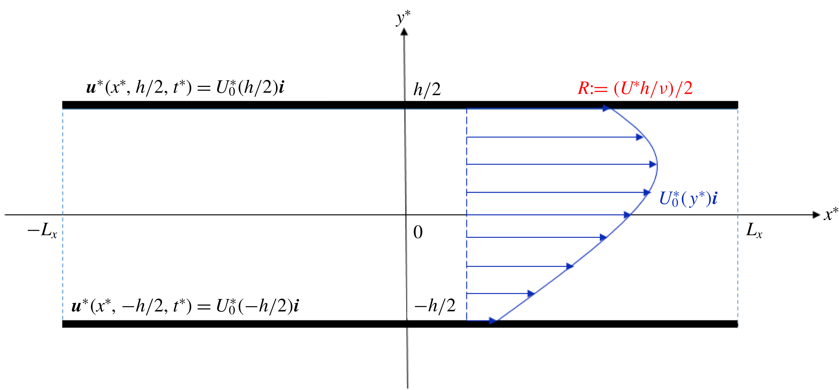
We consider an arbitrary non-zero strictly parallel base steady state of the form
 $\boldsymbol{u}_{0}^{\ast }:=U_{0}^{\ast }(\,y^{\ast })\boldsymbol{i}$
and denote
 $$\begin{eqnarray}U^{\ast }:=\max _{y^{\ast }\in [-h/2,h/2]}|U_{0}^{\ast }(\,y^{\ast })|.\end{eqnarray}$$
The flow velocities at the walls are the following:
 $$\begin{eqnarray}\boldsymbol{u}^{\ast }\left(x^{\ast },\pm \frac{h}{2},t^{\ast }\right)=U_{0}^{\ast }\left(\pm \frac{h}{2}\right)\boldsymbol{i},\end{eqnarray}$$
as illustrated in figure 1.
The dimensional flow system with boundary conditions, in which
 $U_{0}^{\ast }(\,y^{\ast })\boldsymbol{i}$
is an arbitrary base steady state that satisfies (2.1).

We introduce the following dimensionless quantities, in which
 $R$
is the Reynolds number:
 $$\begin{eqnarray}\boldsymbol{u}=\left(\begin{array}{@{}c@{}}u\\ v\end{array}\right):=\frac{1}{U^{\ast }}\boldsymbol{u}^{\ast },\quad \left(\begin{array}{@{}c@{}}x\\ y\end{array}\right):=\frac{2}{h}\left(\begin{array}{@{}c@{}}x^{\ast }\\ y^{\ast }\end{array}\right)\!,\quad t:=\frac{2U^{\ast }}{h}t^{\ast },\quad p:=\frac{p^{\ast }}{U^{\ast 2}},\quad R:=\frac{U^{\ast }h}{2\unicode[STIX]{x1D708}}.\end{eqnarray}$$
Substituting (2.4) into (2.1) we obtain the non-dimensionalized equations
 $$\begin{eqnarray}\left.\begin{array}{@{}c@{}}\displaystyle \frac{\unicode[STIX]{x2202}\boldsymbol{u}}{\unicode[STIX]{x2202}t}+\boldsymbol{u}\boldsymbol{\cdot }\unicode[STIX]{x1D735}\boldsymbol{u}+\unicode[STIX]{x1D735}p=\frac{1}{R}\unicode[STIX]{x1D6FB}^{2}\boldsymbol{u},\\ \unicode[STIX]{x1D735}\boldsymbol{\cdot }\boldsymbol{u}=0.\end{array}\right\}\end{eqnarray}$$
Let
 $L:=2L_{x}/h$
and let
 $U_{0}:=U_{0}^{\ast }/U^{\ast }$
; note that we have
 $|U_{0}(\,y)|\leqslant 1$
for
 $y\in [-1,1]$
. The periodic domain is
 $\unicode[STIX]{x1D6FA}:=[-L,L]\times [-1,1]$
, and
 $\boldsymbol{u}$
is imposed with the rigid-wall boundary condition
 $$\begin{eqnarray}\boldsymbol{u}(x,\pm 1,t)=\left(\begin{array}{@{}c@{}}U_{0}(\pm 1)\\ 0\end{array}\right).\end{eqnarray}$$
Let
 $p_{0}$
be the pressure field corresponding to the base steady state
 $U_{0}(\,y)\boldsymbol{i}$
. It is evident from (2.5) that
 $$\begin{eqnarray}\frac{\unicode[STIX]{x2202}p_{0}}{\unicode[STIX]{x2202}x}=\frac{1}{R}U_{0}^{\prime \prime }(\,y),\quad \frac{\unicode[STIX]{x2202}p_{0}}{\unicode[STIX]{x2202}y}=0.\end{eqnarray}$$
Thus we have
 $$\begin{eqnarray}p_{0}^{\prime \prime }(x)=0=U_{0}^{\prime \prime \prime }(\,y).\end{eqnarray}$$
It implies that
 $U_{0}(\,y)$
is in general a quadratic function, among which
 $U_{0}(\,y)=1-y^{2}$
is viscous planar Poiseuille flow. We restrict our attention to cases where
 $U_{0}^{\prime \prime }(\,y)$
does not change its sign for every
 $y\in (-1,1)$
, namely non-inflectional flows. Without loss of generality, we assume that
 $U_{0}^{\prime \prime }<0$
throughout this study, noting that all results presented henceforth are also valid for the category of flows with
 $U_{0}^{\prime \prime }>0$
. In particular, viscous planar Couette flow has
 $U_{0}(\,y)=y,$
hence it is outside the scope of our study. However, as we shall see, Theorem 3.3 is also applicable to viscous planar Couette flow.
Suppose the following decomposition for a solution
 $\boldsymbol{u}$
of (2.5):
 $$\begin{eqnarray}\boldsymbol{u}=\left(\begin{array}{@{}c@{}}U_{0}(\,y)\\ 0\end{array}\right)+\left(\begin{array}{@{}c@{}}\widetilde{u}(x,y,t)\\ \widetilde{v}(x,y,t)\end{array}\right),\quad p=p_{0}(x)+\widetilde{p}(x,y,t).\end{eqnarray}$$
In accordance with (2.6), the wall boundary conditions on the perturbed fields are
 $$\begin{eqnarray}\left.\left(\begin{array}{@{}c@{}}\widetilde{u}\\ \widetilde{v}\end{array}\right)\right|_{y=\pm 1}=\left(\begin{array}{@{}c@{}}0\\ 0\end{array}\right)\end{eqnarray}$$
together with streamwise periodicity.
For a vorticity form of (2.5), we introduce a stream function
 $\unicode[STIX]{x1D713}(x,y)$
such that
 $u=\unicode[STIX]{x2202}\unicode[STIX]{x1D713}/\unicode[STIX]{x2202}y$
and
 $v=-\unicode[STIX]{x2202}\unicode[STIX]{x1D713}/\unicode[STIX]{x2202}x$
; the corresponding vorticity is
 $\unicode[STIX]{x1D714}:=(\unicode[STIX]{x2202}v/\unicode[STIX]{x2202}x)-(\unicode[STIX]{x2202}u/\unicode[STIX]{x2202}y)=-\unicode[STIX]{x1D6FB}^{2}\unicode[STIX]{x1D713}$
. The vorticity formulation of (2.5) is hence
 $$\begin{eqnarray}\frac{\unicode[STIX]{x2202}\unicode[STIX]{x1D714}}{\unicode[STIX]{x2202}t}+\{\unicode[STIX]{x1D713},\unicode[STIX]{x1D714}\}=\frac{1}{R}\unicode[STIX]{x1D6FB}^{2}\unicode[STIX]{x1D714},\end{eqnarray}$$
in which
 $\{\unicode[STIX]{x1D713},\unicode[STIX]{x1D714}\}:=(\unicode[STIX]{x2202}\unicode[STIX]{x1D713}/\unicode[STIX]{x2202}y)(\unicode[STIX]{x2202}\unicode[STIX]{x1D714}/\unicode[STIX]{x2202}x)-(\unicode[STIX]{x2202}\unicode[STIX]{x1D713}/\unicode[STIX]{x2202}x)(\unicode[STIX]{x2202}\unicode[STIX]{x1D714}/\unicode[STIX]{x2202}y)$
.
Let
 $\unicode[STIX]{x1D713}_{0}$
be the stream function associated with the base flow
 $U_{0}\boldsymbol{i}$
and let
 $\unicode[STIX]{x1D714}_{0}:=-U_{0}^{\prime }=-\unicode[STIX]{x1D713}_{0}^{\prime \prime }$
. Suppose a decomposition for a solution
 $(\unicode[STIX]{x1D713},\unicode[STIX]{x1D714})$
of (2.11) to be
 $\unicode[STIX]{x1D713}=\unicode[STIX]{x1D713}_{0}(\,y)+\widetilde{\unicode[STIX]{x1D713}}(x,y,t)$
and
 $\unicode[STIX]{x1D714}=\unicode[STIX]{x1D714}_{0}(\,y)+\widetilde{\unicode[STIX]{x1D714}}(x,y,t)$
. We enforce streamwise periodicity on
 $\widetilde{\unicode[STIX]{x1D713}}$
. Also, the following boundary conditions on
 $\widetilde{\unicode[STIX]{x1D713}}$
are consistent with (2.10):
 $$\begin{eqnarray}\widetilde{\unicode[STIX]{x1D713}}|_{y=\pm 1}=0,\quad \left.\frac{\unicode[STIX]{x2202}\widetilde{\unicode[STIX]{x1D713}}}{\unicode[STIX]{x2202}y}\right|_{y=\pm 1}=0.\end{eqnarray}$$
Remark.
Note that the wall boundary condition (2.10) is directly inherited from the rigid-wall condition (2.6). From now on, we shall refer to the term ‘no-slip’ wall boundary condition as being the one defined by (2.10). Also, as we shall demonstrate, our major results in the forms of Theorems 3.2 and 3.3 are both valid under more general wall boundary conditions including but not limited to the no-slip wall boundary condition.
3 Linear and global nonlinear stability of viscous planar shear flows
3.1 Viscous extension of Arnold’s inviscid theory to strictly parallel shear flows
In this section, we extend the nonlinear stability theory of Arnold (Reference Arnold1965) on inviscid planar shear flows to viscous planar shear flows subject to two-dimensional disturbances under the no-slip wall boundary condition. As a reminder, note that for the scope of our study on non-inflectional shear flows, we assume without loss of generality that
 $\unicode[STIX]{x1D714}_{0}^{\prime }=-U_{0}^{\prime \prime }>0$
throughout this work.
Denoting the total kinetic energy of a flow field
 $\boldsymbol{u}$
as
 ${\mathcal{E}}:=\frac{1}{2}\int _{\unicode[STIX]{x1D6FA}}\boldsymbol{u}\boldsymbol{\cdot }\boldsymbol{u}\,\text{d}\unicode[STIX]{x1D6FA}$
, the kinetic energy of a base steady state
 $U_{0}\boldsymbol{i}$
is thus
 ${\mathcal{E}}_{0}:=\frac{1}{2}\int _{\unicode[STIX]{x1D6FA}}U_{0}^{2}\,\text{d}\unicode[STIX]{x1D6FA}$
. Let
 $\widetilde{{\mathcal{E}}}:={\mathcal{E}}-{\mathcal{E}}_{0}$
. We define an associated Casimir function to be
 ${\mathcal{C}}_{s}:=\int _{\unicode[STIX]{x1D6FA}}F(\unicode[STIX]{x1D714})\,\text{d}\unicode[STIX]{x1D6FA}$
, where
 $F$
is an arbitrary smooth function. In particular, let
 ${\mathcal{C}}_{s0}:=\int _{\unicode[STIX]{x1D6FA}}F(\unicode[STIX]{x1D714}_{0})\,\text{d}\unicode[STIX]{x1D6FA}$
and
 $\widetilde{{\mathcal{C}}_{s}}:={\mathcal{C}}_{s}-{\mathcal{C}}_{s0}$
.
Following the approach used in Arnold’s study on inviscid shear flows, we need to choose a suitable function
 $F$
that relates
 ${\mathcal{E}}+{\mathcal{C}}_{s}$
to the perturbation fields. Based on the definition of
 $\widetilde{{\mathcal{E}}}$
and the Taylor expansion
 $$\begin{eqnarray}F(\unicode[STIX]{x1D714}_{0}+\widetilde{\unicode[STIX]{x1D714}})=F(\unicode[STIX]{x1D714}_{0})+F^{\prime }(\unicode[STIX]{x1D714}_{0})\widetilde{\unicode[STIX]{x1D714}}+F^{\prime \prime }(\unicode[STIX]{x1D714}_{0}+\unicode[STIX]{x1D702}\widetilde{\unicode[STIX]{x1D714}})\frac{\widetilde{\unicode[STIX]{x1D714}}^{2}}{2},\quad \text{for some}~\unicode[STIX]{x1D702}\in (0,1),\end{eqnarray}$$
we choose
 $F$
to be the function that satisfies the following condition for eliminating the first-order terms in
 $\widetilde{{\mathcal{E}}}+\widetilde{{\mathcal{C}}_{s}}$
:
 $$\begin{eqnarray}U_{0}+F^{\prime \prime }(\unicode[STIX]{x1D714}_{0})\unicode[STIX]{x1D714}_{0}^{\prime }=0,\end{eqnarray}$$
from which we obtain
 $$\begin{eqnarray}\widetilde{{\mathcal{E}}}+\widetilde{{\mathcal{C}}_{s}}=\int _{\unicode[STIX]{x1D6FA}}\frac{1}{2}\widetilde{u}^{2}+\frac{1}{2}\widetilde{v}^{2}+F^{\prime \prime }(\unicode[STIX]{x1D714}_{0}+\unicode[STIX]{x1D702}\widetilde{\unicode[STIX]{x1D714}})\frac{\widetilde{\unicode[STIX]{x1D714}}^{2}}{2}\,\text{d}\unicode[STIX]{x1D6FA}.\end{eqnarray}$$
For the purpose of a conclusive stability analysis, the quadratic form (3.3) needs to be positive definite. This is guaranteed if
 $F^{\prime \prime }$
is a positive-valued function, a requirement that may be fulfilled by the introduction of an appropriate velocity shift to
 $U_{0}$
, as described below.
We introduce a constant velocity shift
 $\overline{U}$
that is to be added to the base steady state’s streamwise velocity profile
 $U_{0}$
, with the observation that
 $\unicode[STIX]{x1D714}_{0}$
as well as all perturbation fields are preserved under such a shift. As such, it enables us to modify (3.2) to be
 $$\begin{eqnarray}U_{0}+\overline{U}+F^{\prime \prime }(\unicode[STIX]{x1D714}_{0})\unicode[STIX]{x1D714}_{0}^{\prime }=0,\end{eqnarray}$$
from which we obtain
 $$\begin{eqnarray}F^{\prime \prime }(\unicode[STIX]{x1D714}_{0})=-\frac{U_{0}(\,y)+\overline{U}}{\unicode[STIX]{x1D714}_{0}^{\prime }}.\end{eqnarray}$$
The positivity of
 $F^{\prime \prime }$
can hence be guaranteed by selecting a sufficiently negative constant shift
 $\overline{U}$
.
Besides the goal of matching for the fixed sign condition on
 $F^{\prime \prime }$
, the inclusion of
 $\overline{U}$
in
 $F^{\prime \prime }(\unicode[STIX]{x1D714}_{0})$
reveals the fact that
 $F^{\prime \prime }(\unicode[STIX]{x1D714}_{0})$
has a freedom due to an arbitrary constant shift. This is built upon the idea of a travelling coordinate system that is moving with a constant velocity relative to the original (stationary) coordinate system. We will base our arguments in § 3.2 on this fact.
Up to this stage, to continue our viscous extension of Arnold’s inviscid theory, we need to ensure also that all first-order terms of the temporal rate of change of
 $\widetilde{{\mathcal{E}}}+\widetilde{{\mathcal{C}}_{s}}$
cancel each other out under the same
 $F$
chosen according to (3.2). Indeed, such a cancellation is ensured by (3.2) too as shown by the following result (see appendix A for a derivation).
Theorem 3.1 (The viscous Arnold’s identity).
The following identity is valid for a strictly parallel viscous planar non-inflectional shear flow
 $U_{0}(\,y)\boldsymbol{i}$
under global nonlinear dynamics enforced by the no-slip wall boundary condition (2.10):
 $$\begin{eqnarray}\frac{1}{2}\frac{\text{d}}{\text{d}t}\int _{\unicode[STIX]{x1D6FA}}[\widetilde{u}^{2}+\widetilde{v}^{2}+F^{\prime \prime }(\unicode[STIX]{x1D714}_{0}+\unicode[STIX]{x1D702}\widetilde{\unicode[STIX]{x1D714}})\widetilde{\unicode[STIX]{x1D714}}^{2}]\,\text{d}\unicode[STIX]{x1D6FA}=-\frac{1}{R}\int _{\unicode[STIX]{x1D6FA}}|\unicode[STIX]{x1D735}\widetilde{u}|^{2}+|\unicode[STIX]{x1D735}\widetilde{v}|^{2}\,\text{d}\unicode[STIX]{x1D6FA}+\frac{1}{R}h(\widetilde{\unicode[STIX]{x1D714}},\unicode[STIX]{x1D709}),\end{eqnarray}$$
where
 $F$
is a function that obeys (3.5) for a sufficiently negative constant
 $\overline{U}$
such that
 $F^{\prime \prime }>0$
,
 $h(\widetilde{\unicode[STIX]{x1D714}},\unicode[STIX]{x1D709})$
is defined as follows:
 $$\begin{eqnarray}\displaystyle h(\widetilde{\unicode[STIX]{x1D714}},\unicode[STIX]{x1D709}) & := & \displaystyle \frac{1}{2}\int _{-L}^{L}\left[F^{\prime \prime \prime }(\unicode[STIX]{x1D714}_{0}+\unicode[STIX]{x1D709}\widetilde{\unicode[STIX]{x1D714}})\widetilde{\unicode[STIX]{x1D714}}^{2}\left(\unicode[STIX]{x1D714}_{0}^{\prime }+\unicode[STIX]{x1D709}\frac{\unicode[STIX]{x2202}\widetilde{\unicode[STIX]{x1D714}}}{\unicode[STIX]{x2202}y}\right)+2F^{\prime \prime }(\unicode[STIX]{x1D714}_{0}+\unicode[STIX]{x1D709}\widetilde{\unicode[STIX]{x1D714}})\widetilde{\unicode[STIX]{x1D714}}\frac{\unicode[STIX]{x2202}\widetilde{\unicode[STIX]{x1D714}}}{\unicode[STIX]{x2202}y}\right]_{y=-1}^{y=1}\text{d}x\nonumber\\ \displaystyle & & \displaystyle -\,\frac{1}{2}\int _{\unicode[STIX]{x1D6FA}}\left\{F^{\prime \prime \prime \prime }(\unicode[STIX]{x1D714}_{0}+\unicode[STIX]{x1D709}\widetilde{\unicode[STIX]{x1D714}})\widetilde{\unicode[STIX]{x1D714}}^{2}\left[\left(\unicode[STIX]{x1D709}\frac{\unicode[STIX]{x2202}\widetilde{\unicode[STIX]{x1D714}}}{\unicode[STIX]{x2202}x}\right)^{2}+\left(\unicode[STIX]{x1D714}_{0}^{\prime }+\unicode[STIX]{x1D709}\frac{\unicode[STIX]{x2202}\widetilde{\unicode[STIX]{x1D714}}}{\unicode[STIX]{x2202}y}\right)^{2}\right]\right.\nonumber\\ \displaystyle & & \displaystyle +\,4F^{\prime \prime \prime }(\unicode[STIX]{x1D714}_{0}+\unicode[STIX]{x1D709}\widetilde{\unicode[STIX]{x1D714}})\widetilde{\unicode[STIX]{x1D714}}\left[\unicode[STIX]{x1D709}\left(\frac{\unicode[STIX]{x2202}\widetilde{\unicode[STIX]{x1D714}}}{\unicode[STIX]{x2202}x}\right)^{2}+\left(\unicode[STIX]{x1D714}_{0}^{\prime }+\unicode[STIX]{x1D709}\frac{\unicode[STIX]{x2202}\widetilde{\unicode[STIX]{x1D714}}}{\unicode[STIX]{x2202}y}\right)\frac{\unicode[STIX]{x2202}\widetilde{\unicode[STIX]{x1D714}}}{\unicode[STIX]{x2202}y}\right]\nonumber\\ \displaystyle & & \displaystyle +\!\left.2F^{\prime \prime }(\unicode[STIX]{x1D714}_{0}+\unicode[STIX]{x1D709}\widetilde{\unicode[STIX]{x1D714}})|\unicode[STIX]{x1D735}\widetilde{\unicode[STIX]{x1D714}}|^{2}\vphantom{\left[\left(\unicode[STIX]{x1D714}_{0}^{\prime }+\unicode[STIX]{x1D709}\frac{\unicode[STIX]{x2202}\widetilde{\unicode[STIX]{x1D714}}}{\unicode[STIX]{x2202}y}\right)^{2}\right]}\right\}\text{d}\unicode[STIX]{x1D6FA},\end{eqnarray}$$
and
 $\unicode[STIX]{x1D702}(x,y,t),\unicode[STIX]{x1D709}(x,y,t)$
are two functions that depend upon
 $\widetilde{\unicode[STIX]{x1D714}}$
with range
 $(0,1)$
.
We have so far extended Arnold’s nonlinear stability theory of inviscid parallel shear flows to viscous parallel shear flows. The basic physics revealed by Arnold’s inviscid theory indicates that there is no physical mechanism which is capable of supporting the growth of the perturbation’s energy and vorticity, as shown by Arnold’s function on the left-hand side of (3.6). The above result demonstrates that the same holds true for viscous shear flows, namely all the terms related to the inviscid mechanism cancel each other out perfectly and the remaining terms are explicitly viscous. Theorem 3.1 is new and it serves as a basis for a number of results presented in subsequent sections.
3.2 An alternative path to the enstrophy identity by Synge (Reference Synge1938)
Let us reduce the complexity of the remainder term
 $h(\widetilde{\unicode[STIX]{x1D714}},\unicode[STIX]{x1D709})$
in Theorem 3.1 for now by considering its linearized form, with those disturbance terms that are higher than the second-order removed. Therefrom, we obtain the following:
 $$\begin{eqnarray}\displaystyle & & \displaystyle \frac{1}{2}\frac{\text{d}}{\text{d}t}\int _{\unicode[STIX]{x1D6FA}}\left[\widetilde{u}^{2}+\widetilde{v}^{2}+F^{\prime \prime }(\unicode[STIX]{x1D714}_{0})\widetilde{\unicode[STIX]{x1D714}}^{2}\right]\text{d}\unicode[STIX]{x1D6FA}=-\frac{1}{R}\int _{\unicode[STIX]{x1D6FA}}|\unicode[STIX]{x1D735}\widetilde{u}|^{2}+|\unicode[STIX]{x1D735}\widetilde{v}|^{2}\,\text{d}\unicode[STIX]{x1D6FA}\nonumber\\ \displaystyle & & \displaystyle \quad +\frac{1}{2R}\int _{-L}^{L}\left[F^{\prime \prime \prime }(\unicode[STIX]{x1D714}_{0})\unicode[STIX]{x1D714}_{0}^{\prime }\widetilde{\unicode[STIX]{x1D714}}^{2}+2F^{\prime \prime }(\unicode[STIX]{x1D714}_{0})\widetilde{\unicode[STIX]{x1D714}}\frac{\unicode[STIX]{x2202}\widetilde{\unicode[STIX]{x1D714}}}{\unicode[STIX]{x2202}y}\right]_{y=-1}^{y=1}\text{d}x\nonumber\\ \displaystyle & & \displaystyle \quad -\,\frac{1}{2R}\int _{\unicode[STIX]{x1D6FA}}\left\{F^{\prime \prime \prime \prime }(\unicode[STIX]{x1D714}_{0})\unicode[STIX]{x1D714}_{0}^{\prime 2}\widetilde{\unicode[STIX]{x1D714}}^{2}+4F^{\prime \prime \prime }(\unicode[STIX]{x1D714}_{0})\unicode[STIX]{x1D714}_{0}^{\prime }\widetilde{\unicode[STIX]{x1D714}}\frac{\unicode[STIX]{x2202}\widetilde{\unicode[STIX]{x1D714}}}{\unicode[STIX]{x2202}y}+2F^{\prime \prime }(\unicode[STIX]{x1D714}_{0})|\unicode[STIX]{x1D735}\widetilde{\unicode[STIX]{x1D714}}|^{2}\right\}\text{d}\unicode[STIX]{x1D6FA}.\end{eqnarray}$$
For further simplification of (3.8), we elaborate the observation made through (3.5) that
 $F^{\prime \prime }(\unicode[STIX]{x1D714}_{0})$
has a freedom due to an arbitrary constant shift
 $\overline{U}$
, together with the fact that
 $\unicode[STIX]{x1D714}_{0}^{\prime }$
is a positive constant due to the strict parallelism assumption on
 $U_{0}$
as enforced by (2.8).
Specifically, as we observed through (3.5),
 $F^{\prime \prime }(\unicode[STIX]{x1D714}_{0})$
has a freedom due to an arbitrary constant shift
 $\overline{U}$
. Differentiating both sides of (3.5) with respect to
 $y$
, with the observation that
 $\unicode[STIX]{x1D714}_{0}^{\prime }$
is a constant, we have
 $$\begin{eqnarray}F^{\prime \prime \prime }(\unicode[STIX]{x1D714}_{0})=\frac{\unicode[STIX]{x1D714}_{0}}{\unicode[STIX]{x1D714}_{0}^{\prime 2}},\quad F^{\prime \prime \prime \prime }(\unicode[STIX]{x1D714}_{0})=\frac{1}{\unicode[STIX]{x1D714}_{0}^{\prime 2}}.\end{eqnarray}$$
Substituting (3.5) and (3.9) into (3.8), and dividing both sides of the resulting identiy by
 $-\overline{U}$
we obtain
 $$\begin{eqnarray}\displaystyle & & \displaystyle \frac{1}{2}\frac{\text{d}}{\text{d}t}\int _{\unicode[STIX]{x1D6FA}}\left[-\frac{\widetilde{u}^{2}+\widetilde{v}^{2}}{\overline{U}}+\frac{U_{0}(\,y)+\overline{U}}{\unicode[STIX]{x1D714}_{0}^{\prime }(\,y)\overline{U}}\widetilde{\unicode[STIX]{x1D714}}^{2}\right]\text{d}\unicode[STIX]{x1D6FA}=\frac{1}{R}\int _{\unicode[STIX]{x1D6FA}}\frac{|\unicode[STIX]{x1D735}\widetilde{u}|^{2}+|\unicode[STIX]{x1D735}\widetilde{v}|^{2}}{\overline{U}}\,\text{d}\unicode[STIX]{x1D6FA}\nonumber\\ \displaystyle & & \displaystyle \quad +\,\frac{1}{2R}\int _{-L}^{L}\left[-\frac{\unicode[STIX]{x1D714}_{0}(\,y)}{\unicode[STIX]{x1D714}_{0}^{\prime }(\,y)\overline{U}}\widetilde{\unicode[STIX]{x1D714}}^{2}+2\frac{U_{0}(\,y)+\overline{U}}{\unicode[STIX]{x1D714}_{0}^{\prime }(\,y)\overline{U}}\widetilde{\unicode[STIX]{x1D714}}\frac{\unicode[STIX]{x2202}\widetilde{\unicode[STIX]{x1D714}}}{\unicode[STIX]{x2202}y}\right]_{y=-1}^{y=1}\text{d}x\nonumber\\ \displaystyle & & \displaystyle \quad -\,\frac{1}{2R}\int _{\unicode[STIX]{x1D6FA}}\left\{-\frac{\widetilde{\unicode[STIX]{x1D714}}^{2}}{\overline{U}}-4\frac{\unicode[STIX]{x1D714}_{0}(\,y)}{\unicode[STIX]{x1D714}_{0}^{\prime }(\,y)\overline{U}}\widetilde{\unicode[STIX]{x1D714}}\frac{\unicode[STIX]{x2202}\widetilde{\unicode[STIX]{x1D714}}}{\unicode[STIX]{x2202}y}+2\frac{U_{0}(\,y)+\overline{U}}{\unicode[STIX]{x1D714}_{0}^{\prime }(\,y)\overline{U}}|\unicode[STIX]{x1D735}\widetilde{\unicode[STIX]{x1D714}}|^{2}\right\}\text{d}\unicode[STIX]{x1D6FA}.\end{eqnarray}$$
Taking the limit as
 $\overline{U}\rightarrow -\infty$
in (3.10) and then dividing out the constant common weight factor
 $1/\unicode[STIX]{x1D714}_{0}^{\prime }$
on both sides of the resulting equality leads to the following identity:
 $$\begin{eqnarray}\frac{1}{2}\frac{\text{d}}{\text{d}t}\int _{\unicode[STIX]{x1D6FA}}\widetilde{\unicode[STIX]{x1D714}}^{2}\,\text{d}\unicode[STIX]{x1D6FA}=\frac{1}{R}\int _{-L}^{L}\left[\widetilde{\unicode[STIX]{x1D714}}\frac{\unicode[STIX]{x2202}\widetilde{\unicode[STIX]{x1D714}}}{\unicode[STIX]{x2202}y}\right]_{y=-1}^{y=1}\text{d}x-\frac{1}{R}\int _{\unicode[STIX]{x1D6FA}}|\unicode[STIX]{x1D735}\widetilde{\unicode[STIX]{x1D714}}|^{2}\,\text{d}\unicode[STIX]{x1D6FA},\end{eqnarray}$$
where
 $\widetilde{\unicode[STIX]{x1D714}}$
is determined by the linear dynamics under the no-slip wall boundary condition (2.10).
Identity (3.11) was first discovered by Synge (Reference Synge1938) within the framework of the classical normal-mode analysis in which perturbations are restricted to exponential growth/decay modes. Fraternale et al. (Reference Fraternale, Domenicale, Staffilani and Tordella2018) recently extended Synge’s result to include general infinitesimal disturbances, and obtained (3.11) explicitly. Our alternative derivation presented above establishes a natural connection between the viscous Arnold’s identity and (3.11). Moreover, our alternative derivation signals the potential of using the viscous Arnold’s identity to find new identities that quantify the perturbation’s enstrophy. Regarding such potential as a strategy gives rise to much of the work presented in §§ 3.3 and 3.4.
The quantity
 $\int _{\unicode[STIX]{x1D6FA}}\widetilde{\unicode[STIX]{x1D714}}^{2}\,\text{d}\unicode[STIX]{x1D6FA}$
is commonly referred to as the perturbation’s enstrophy over the domain
 $\unicode[STIX]{x1D6FA}$
. It is worth mentioning that there is rather limited study in literature that aims to explore the physical mechanism of shear flow stability from the perspective of enstrophy (Fraternale et al.
Reference Fraternale, Domenicale, Staffilani and Tordella2018).
An evident observation that can be made immediately based on (3.11) is that the perturbation’s enstrophy can only be produced at the walls, and it dissipates inside the flow domain. However, one cannot draw any further conclusion based on (3.11) alone about the production/dissipation of the perturbation’s enstrophy. With the aid of numerical computation, we will address this question in § 4.1 in the context of planar Poiseuille flow.
We have restricted our attention so far to strictly parallel shear flows under the no-slip wall boundary condition. In the next two sections, we will relax the parallelism assumption and/or relax the no-slip wall boundary condition to arrive at two additional novel results of this study. As we shall see, both of the forthcoming results have their roots in Theorem 3.1.
3.3 A weighted disturbance’s enstrophy identity for non-parallel shear flows
As we observed in the derivation procedure of (3.11), we needed to divide out the constant common weight factor
 $1/\unicode[STIX]{x1D714}_{0}^{\prime }$
on both sides of the resulting equality to finally obtain (3.11). Apparently, the constant weight factor
 $1/\unicode[STIX]{x1D714}_{0}^{\prime }$
that originally appeared on both sides of (3.11) played no practical role. However, it suggests a weighted enstrophy identity that might be valid for a broader category of shear flows which are not strictly parallel. Note that such a weight factor corresponding to a non-parallel shear flow is no longer a constant.
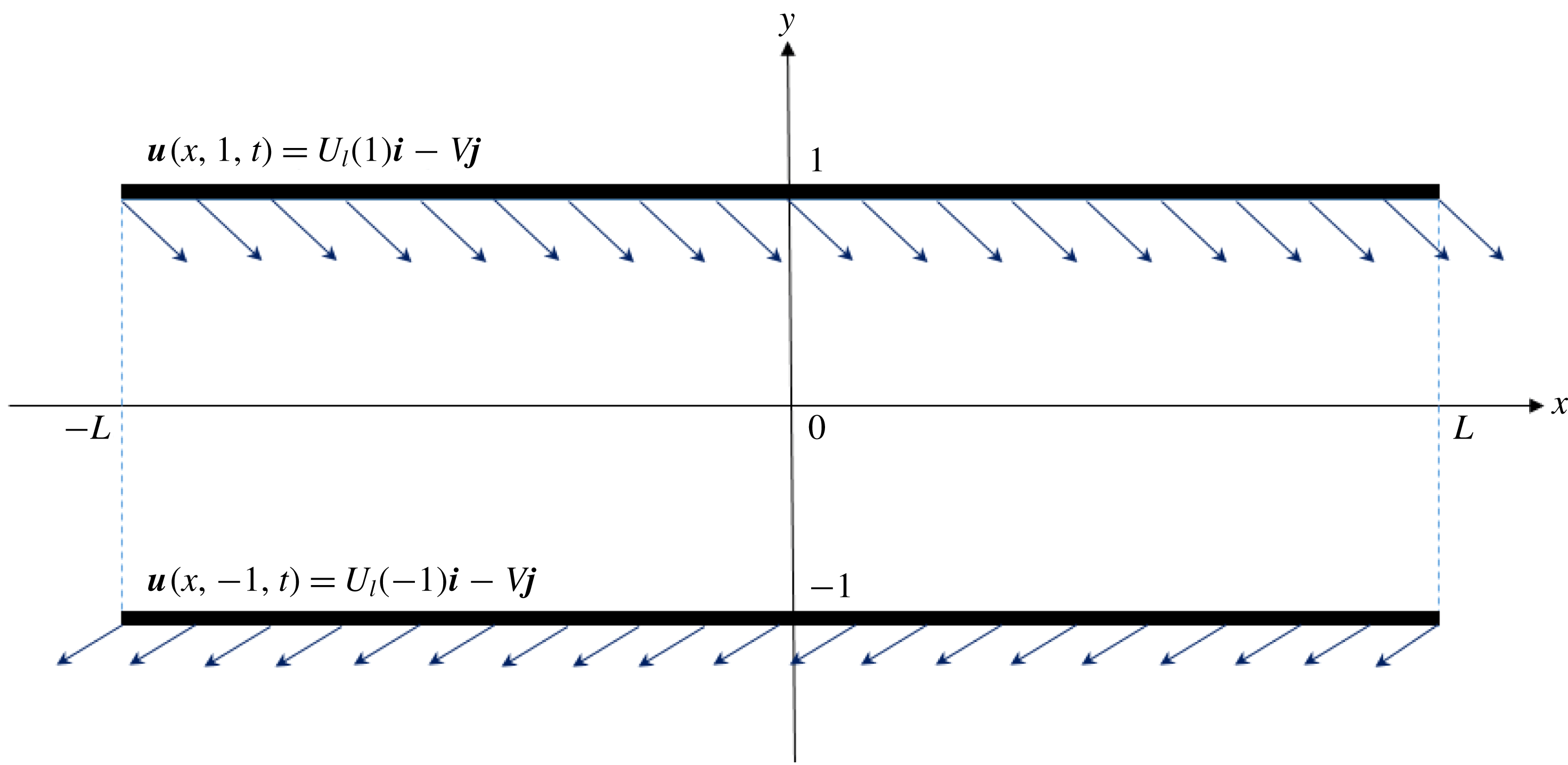
For a streamwise translation-invariant shear flow that is not strictly parallel, such as a shear layer subject to uniform injection and suction of fluid through its walls, its streamwise velocity profile is in general non-inflectional. A sketch of the boundaries and wall boundary conditions for a flow of this kind is illustrated in figure 2. We present the following weighted perturbation’s enstrophy identity for such flows, which is inspired by the viscous Arnold’s identity (3.6) and (3.7), see appendix B for a direct derivation.
Sketch of the boundaries and wall boundary conditions for a streamwise translation-invariant non-parallel shear flow with uniform boundary injection and suction imposed. The streamwise velocity component is
 $U_{l}(\,y)$
, and the constant rate of injection (through the top wall) and suction (through the bottom wall) are both
 $-V$
.

Theorem 3.2 (A weighted perturbation’s enstrophy identity).
Let
 $U_{l}(\,y)\boldsymbol{i}-V\boldsymbol{j}$
be a steady-state velocity field of a viscous shear flow that fulfils (2.5), where
 $V$
is a constant. Suppose that at each wall either of the following two categories of boundary conditions is imposed:
(i)
 $\widetilde{v}=0$
and another arbitrarily prescribed condition on a perturbation field;
(ii)
$\widetilde{u}=0$
and another arbitrarily prescribed condition on a perturbation field.


Denote its vorticity by
 $\unicode[STIX]{x1D714}_{l}:=-U_{l}^{\prime }$
, assuming that
 $\unicode[STIX]{x1D714}_{l}^{\prime }\neq 0$
for
 $y\in (0,1)$
. We have
 $$\begin{eqnarray}\frac{1}{2}\frac{\text{d}}{\text{d}t}\int _{\unicode[STIX]{x1D6FA}}\frac{1}{\unicode[STIX]{x1D714}_{l}^{\prime }}\widetilde{\unicode[STIX]{x1D714}}^{2}\,\text{d}\unicode[STIX]{x1D6FA}=\frac{1}{R}\int _{-L}^{L}\left[\frac{1}{\unicode[STIX]{x1D714}_{l}^{\prime }}\widetilde{\unicode[STIX]{x1D714}}\frac{\unicode[STIX]{x2202}\widetilde{\unicode[STIX]{x1D714}}}{\unicode[STIX]{x2202}y}\right]_{y=-1}^{y=1}\text{d}x-\frac{1}{R}\int _{\unicode[STIX]{x1D6FA}}\frac{1}{\unicode[STIX]{x1D714}_{l}^{\prime }}|\unicode[STIX]{x1D735}\widetilde{\unicode[STIX]{x1D714}}|^{2}\,\text{d}\unicode[STIX]{x1D6FA},\end{eqnarray}$$
in which the perturbation’s vorticity
 $\widetilde{\unicode[STIX]{x1D714}}$
is determined by linear dynamics.
Theorem 3.2 provides us with a novel weighted identity for streamwise translation-invariant shear flows. We present the following flow example taken from Doering, Spiegel & Worthing (Reference Doering, Spiegel and Worthing2000) for illustrating an application of Theorem 3.2.
Example 3.1. Viscous planar Couette flow with injection and suction. Consider planar Couette flow with
 $U_{0}(\,y)=y$
. After a constant injection and suction rate
 $-V$
through the walls is imposed, its original linear streamwise velocity profile would then be disturbed, and a base steady state of the new flow system is of the form
 $U_{l}(\,y)\boldsymbol{i}-V\boldsymbol{j}$
, with
 $$\begin{eqnarray}U_{l}(\,y):=\frac{2-2\exp [-RV(\,y+1)]}{1-\exp (-2RV)}-1.\end{eqnarray}$$
Note that
 $U_{l}(\,y)\rightarrow U_{0}(\,y)=y$
when
 $V\rightarrow 0$
. The corresponding weight function is
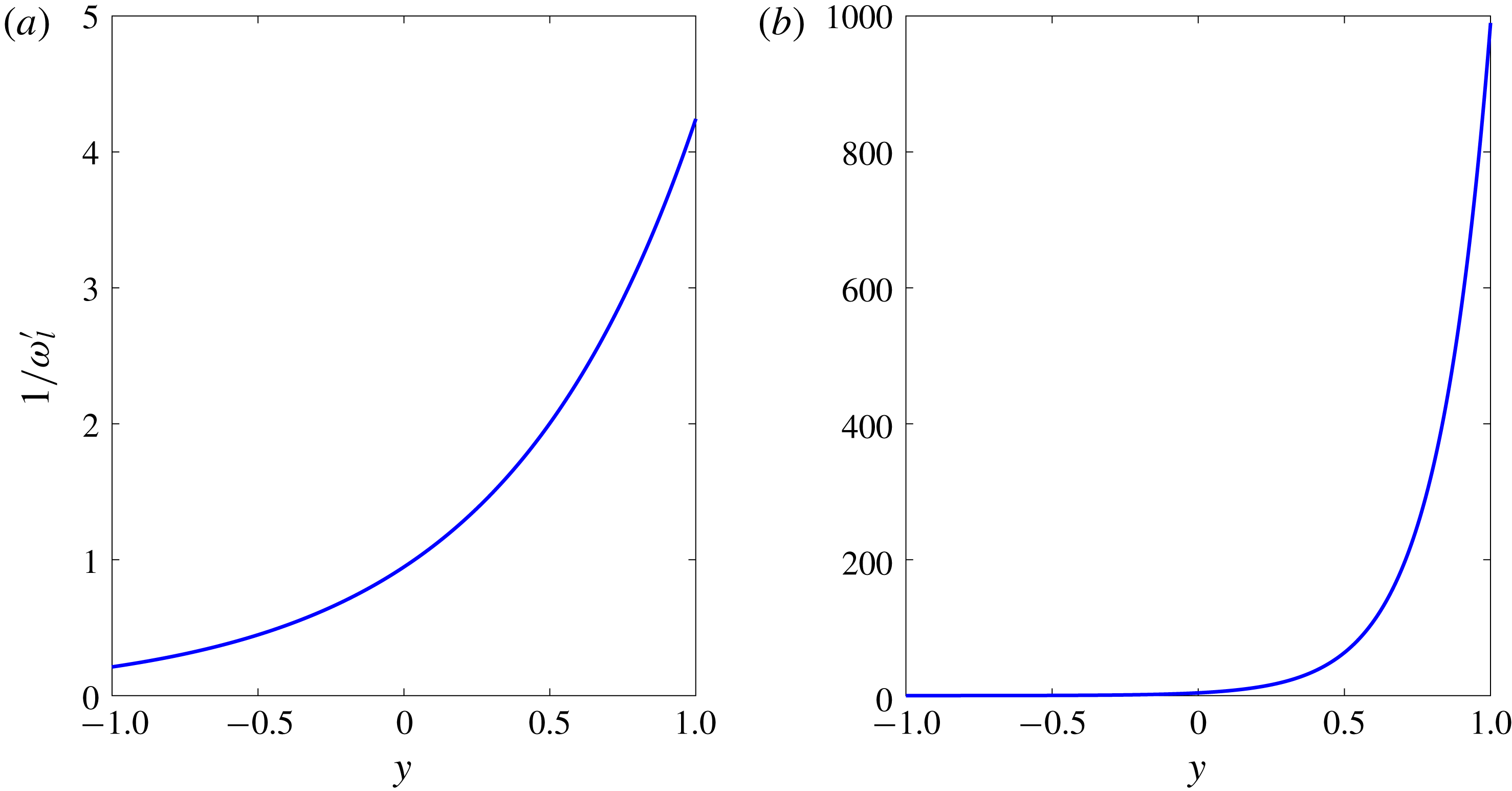
 $$\begin{eqnarray}\frac{1}{\unicode[STIX]{x1D714}_{l}^{\prime }(\,y)}=-\frac{1}{U_{l}^{\prime \prime }(\,y)}=\frac{1-\exp (-2RV)}{2R^{2}V^{2}}\exp [RV(\,y+1)].\end{eqnarray}$$
Plots of the weight function
 $1/\unicode[STIX]{x1D714}_{l}^{\prime }$
for viscous planar Couette flow with wall boundary injection and suction at
 $R=10^{6}$
and (a)
 $V=1.5\times 10^{-6}$
, (b)
 $V=5.5\times 10^{-6}$
.

Plots of the weight function at
 $R=10^{6}$
with
 $V=1.5\times 10^{-6}$
and
 $V=5.5\times 10^{-6}$
are shown in figures 3(a) and 3(b), respectively. The weights in both cases exhibit relatively large magnitudes in a vicinity of the upper wall, whereas their values at the lower wall are relatively negligible. The presence of the weight function reveals a significant fact, that the upper wall plays a much more dominant role than the lower in terms of their influence on the stability of the flow. This is especially clear in the case
 $V=5.5\times 10^{-6}$
, in which the magnitude of the weight function reaches an exceedingly high magnitude of nearly
 $O(10^{3})$
at the upper wall, whereas it remains of
 $O(1)$
at the lower wall.
3.4 Imposing wall boundary conditions on (3.11) under global nonlinear dynamics
Let us take a step back to our study on strictly parallel non-inflectional shear flows. With the observation that
 $\unicode[STIX]{x1D714}_{0}^{\prime }$
is a non-zero constant, applying the aforementioned procedure in § 3.2 used to derive (3.11) under linear dynamics to the fully nonlinear viscous Arnold’s identity (3.6) and (3.7) brings one to exactly the same identity as (3.11). Therefore, equation (3.11) also holds for global nonlinear dynamics under the no-slip wall boundary condition. This is a direct consequence of the global nonlinear nature of the viscous Arnold’s identity.
In fact, as noted in the work by Fraternale et al. (Reference Fraternale, Domenicale, Staffilani and Tordella2018) (see also appendix C of Tsinober Reference Tsinober2001), the temporal rate of change of the perturbation’s enstrophy quantified by (3.11) is independent of the disturbance’s amplitude. Thus, the perturbation’s dynamics is governed by linear mechanisms only. Physically, this evidence is related to the lack of vortex stretching in two dimensions. Fraternale et al. (Reference Fraternale, Domenicale, Staffilani and Tordella2018) adopted this evidence to justify the usage of linearized equation (3.11) for seeking improved bounds (in terms of the Reynolds number) on the global nonlinear stability of planar Couette flow and planar Poiseuille flow.
Taking the above evidence as inspiration, we rigorously examined the validity of (3.11) for strictly parallel shear flows under global nonlinear dynamics imposed with two categories of wall boundary conditions, and we obtained the following result (see appendix C for a derivation).
Theorem 3.3. Let
 $\widetilde{\unicode[STIX]{x1D714}}$
be the perturbation’s vorticity of a strictly parallel viscous planar shear flow
 $U_{0}(\,y)\boldsymbol{i}$
(
 $\unicode[STIX]{x1D714}_{0}^{\prime }(\,y)$
is a constant). Suppose that at each wall either of the following two categories of boundary conditions is imposed:
(i)
$\widetilde{v}=0$
and another arbitrarily prescribed condition on a perturbation field;(ii)
$\widetilde{u}=0$
and
$\widetilde{\unicode[STIX]{x1D714}}=0$
.


The temporal evolution of the perturbation’s enstrophy is then still governed by (3.11) under global nonlinear dynamics.
The above result presents two categories of wall boundary conditions that include, but are not limited to, the no-slip wall boundary condition (2.10). The first category of boundary conditions require that
 $\widetilde{v}=0$
at the walls. It hence provides one with the freedom to impose an additional wall boundary condition on a disturbance field to make the problem well-posed. Such freedom in the choice of another arbitrary wall boundary condition gives rise to the potential of controlling finite-amplitude perturbation fields at the walls.
The second category of wall conditions are compatible with the vorticity flow equations (2.11). Note that since
 $\widetilde{u}$
is prescribed at the walls, the other wall condition on
 $\widetilde{\unicode[STIX]{x1D714}}$
may be matched through controls on
 $\widetilde{v}$
at the walls. Note also that the application of (3.11) to this case implies immediately the global nonlinear stability of the base flow, and it leads to an upper bound for the decay rate of the disturbance’s enstrophy. We elaborate this through the following example.
Example 3.2. Consider the viscous planar Poiseuille flow
 $(1-y^{2})\boldsymbol{i}$
with its no-slip wall boundary condition
 $$\begin{eqnarray}\left.\left(\begin{array}{@{}c@{}}u\\ v\end{array}\right)\right|_{y=\pm 1}=\left(\begin{array}{@{}c@{}}0\\ 0\end{array}\right)\end{eqnarray}$$
replaced by
 $$\begin{eqnarray}\left.\left(\begin{array}{@{}c@{}}u\\ \unicode[STIX]{x1D714}\end{array}\right)\right|_{y=\pm 1}=\left(\begin{array}{@{}c@{}}0\\ \pm 2\end{array}\right)\quad \text{or}\quad \left.\left(\begin{array}{@{}c@{}}v\\ \unicode[STIX]{x1D714}\end{array}\right)\right|_{y=\pm 1}=\left(\begin{array}{@{}c@{}}0\\ \pm 2\end{array}\right).\end{eqnarray}$$
Note that
 $U_{0}(\,y)\boldsymbol{i}$
remains the base steady state under the new wall boundary conditions (3.16), because
 $\unicode[STIX]{x1D714}_{0}(\,y)=-U_{0}^{\prime }(\,y)$
.
Since the values of
 $\unicode[STIX]{x1D714}$
are prescribed to be those of
 $\unicode[STIX]{x1D714}_{0}$
at
 $y=\pm 1$
, it implies that
 $\widetilde{\unicode[STIX]{x1D714}}=0$
at the walls. Application of Theorem 3.3 into this case leads to the deduction that
 $$\begin{eqnarray}\frac{1}{2}\frac{\text{d}}{\text{d}t}\int _{\unicode[STIX]{x1D6FA}}\widetilde{\unicode[STIX]{x1D714}}^{2}\,\text{d}\unicode[STIX]{x1D6FA}=-\frac{1}{R}\int _{\unicode[STIX]{x1D6FA}}|\unicode[STIX]{x1D735}\widetilde{\unicode[STIX]{x1D714}}|^{2}\,\text{d}\unicode[STIX]{x1D6FA}<0,\quad \text{for}~\widetilde{\unicode[STIX]{x1D714}}\neq 0.\end{eqnarray}$$
Equation (3.17) implies that under the wall boundary condition (3.16), any given initial finite-amplitude perturbation of the viscous planar Poiseuille flow must decay with respect to time. For an estimation of the decay rate, we introduce the following Poincaré inequality that is compatible with the streamwise periodic condition on
 $\widetilde{\unicode[STIX]{x1D714}}$
and
 $\widetilde{\unicode[STIX]{x1D714}}=0$
at the walls (Adams & Fournier Reference Adams and Fournier2003):
 $$\begin{eqnarray}\int _{\unicode[STIX]{x1D6FA}}\widetilde{\unicode[STIX]{x1D714}}^{2}\,\text{d}\unicode[STIX]{x1D6FA}\leqslant M\int _{\unicode[STIX]{x1D6FA}}|\unicode[STIX]{x1D735}\widetilde{\unicode[STIX]{x1D714}}|^{2}\,\text{d}\unicode[STIX]{x1D6FA},\end{eqnarray}$$
where
 $M$
is a positive constant depending upon the domain
 $\unicode[STIX]{x1D6FA}$
. To be precise, the constant
 $M$
is determined by the Rayleigh quotient
 $$\begin{eqnarray}M:=\left[\min _{\widetilde{\unicode[STIX]{x1D714}}}{\displaystyle \frac{\displaystyle \int _{\unicode[STIX]{x1D6FA}}|\unicode[STIX]{x1D735}\widetilde{\unicode[STIX]{x1D714}}|^{2}\,\text{d}\unicode[STIX]{x1D6FA}}{\displaystyle \int _{\unicode[STIX]{x1D6FA}}\widetilde{\unicode[STIX]{x1D714}}^{2}\,\text{d}\unicode[STIX]{x1D6FA}}}\right]^{-1},\end{eqnarray}$$
in which the minimization process is taken over all perturbation fields
 $\widetilde{\unicode[STIX]{x1D714}}$
that are admissible with the boundary conditions. By using (3.18), we find an upper bound for the right-hand side of (3.17) to be
 $$\begin{eqnarray}\frac{\text{d}\widetilde{\mathscr{W}}}{\text{d}t}\leqslant -\frac{2}{MR}\widetilde{\mathscr{W}},\end{eqnarray}$$
where
 $\widetilde{\mathscr{W}}(t):=\int _{\unicode[STIX]{x1D6FA}}[\widetilde{\unicode[STIX]{x1D714}}(x,y,t)]^{2}\,\text{d}\unicode[STIX]{x1D6FA}$
. It yields the following analytical estimation of the upper bound for the decay of the perturbation’s enstrophy
 $\widetilde{\mathscr{W}}$
:
 $$\begin{eqnarray}\widetilde{\mathscr{W}}(t)\leqslant \widetilde{\mathscr{W}}(0)\text{e}^{-2t/(M_{}R)},\quad \text{for all times}~t\geqslant 0.\end{eqnarray}$$
We have therefore established the global nonlinear stability for the flow.
The wall condition
 $(\widetilde{v},\unicode[STIX]{x2202}\widetilde{u}/\unicode[STIX]{x2202}y)=(0,0)$
(i.e.
 $\widetilde{\unicode[STIX]{x1D714}}=0$
) is commonly referred to as the free-slip condition. Waleffe & Kerswell (Reference Waleffe and Kerswell2011) reviewed and studied the role of wall boundary conditions in the stability of strictly parallel shear flows and found that the flows are linearly stable under the free-slip condition.
We would like to remark that the disturbance’s vorticity
 $\widetilde{\unicode[STIX]{x1D714}}$
at the walls is generally unknown for other wall boundary conditions, in particular for the no-slip wall condition. Thus, additional constraints on the disturbance fields are in general necessary to enable an estimate of the boundary term in (3.11). Fraternale et al. (Reference Fraternale, Domenicale, Staffilani and Tordella2018) conducted a study on viscous planar Poiseuille flow and planar Couette flow with the no-slip wall condition imposed for both flows, through the incorporation of a variational constraint, and improved marginal stability bounds were concluded for these flows.
An implementation of the proposed boundary conditions in Theorem 3.3 may lead to effective flow control methodologies. We shall present a control scheme in § 4.2 that transitions the wall settings from the no-slip condition to the free-slip condition.
4 Preliminary interpretation of linear instability/stability and wall boundary vorticity control for viscous planar Poiseuille flow
In the next two sections, we investigate distributions of the perturbation’s enstrophy at/between the walls within the classical normal modal framework. The investigation includes a variety of flow parameters and wall conditions, aimed at acquiring a more quantitative understanding of the production/dissipation mechanisms of the perturbation’s enstrophy. Viscous planar Poiseuille flow is selected to be the base state for our investigation. The no-slip wall condition is imposed throughout § 4.1, followed by a flow control scheme that transitions the no-slip condition to the free-slip condition in § 4.2.
4.1 Interpretation of linear instability/stability under the no-slip wall condition
For a classical normal-mode analysis, we propose perturbations to be of the following form:
 $$\begin{eqnarray}\left(\begin{array}{@{}c@{}}\widetilde{\unicode[STIX]{x1D713}}\\ \widetilde{u}\\ \widetilde{v}\\ \widetilde{\unicode[STIX]{x1D714}}\end{array}\right)=\left(\begin{array}{@{}c@{}}\unicode[STIX]{x1D719}(\,y)\\ \widehat{u}(\,y)\\ \widehat{v}(\,y)\\ \widehat{\unicode[STIX]{x1D714}}(\,y)\end{array}\right)\exp [\text{i}\unicode[STIX]{x1D6FC}(x-ct)],\quad \text{with}\left(\begin{array}{@{}c@{}}\widehat{u}\\ \widehat{v}\\ \widehat{\unicode[STIX]{x1D714}}\end{array}\right)=\left(\begin{array}{@{}c@{}}\unicode[STIX]{x1D719}^{\prime }\\ -\text{i}\unicode[STIX]{x1D6FC}\unicode[STIX]{x1D719}\\ \unicode[STIX]{x1D6FC}^{2}\unicode[STIX]{x1D719}-\unicode[STIX]{x1D719}^{\prime \prime }\end{array}\right),\end{eqnarray}$$
in which
 $\unicode[STIX]{x1D6FC}$
denotes the positive spatial wavenumber of the perturbations, and
 $c$
denotes the complex phase velocity (
 $c:=c_{r}+\text{i}c_{i}$
,
 $\text{i}^{2}=-1$
).
Substituting (4.1) into the linearized equation (B 1) with
 $V\rightarrow 0$
and
 $U_{l}$
replaced by
 $U_{0}$
we obtain the standard Orr–Sommerfeld stability equation
 $$\begin{eqnarray}(\text{i}\unicode[STIX]{x1D6FC}R)^{-1}(\mathscr{D}^{2}-\unicode[STIX]{x1D6FC}^{2})^{2}\unicode[STIX]{x1D719}=(U_{0}-c)(\mathscr{D}^{2}-\unicode[STIX]{x1D6FC}^{2})\unicode[STIX]{x1D719}-U_{0}^{\prime \prime }\unicode[STIX]{x1D719},\end{eqnarray}$$
in which
 $\mathscr{D}:=\text{d}/\text{d}y$
. In this section, we impose (4.2) with the no-slip wall boundary condition
 $$\begin{eqnarray}\widehat{u}(\pm 1)=0=\widehat{v}(\pm 1).\end{eqnarray}$$
The growth rate of the perturbations is hence computed from (3.11) to be
 $$\begin{eqnarray}c_{i}=\left.\frac{1}{\unicode[STIX]{x1D6FC}R}\left(\int _{-L}^{L}\left[\text{Re}(\widetilde{\unicode[STIX]{x1D714}})\frac{\unicode[STIX]{x2202}\,\text{Re}(\widetilde{\unicode[STIX]{x1D714}})}{\unicode[STIX]{x2202}y}\right]_{y=-1}^{y=1}\text{d}x-\int _{\unicode[STIX]{x1D6FA}}|\unicode[STIX]{x1D735}\text{Re}(\widetilde{\unicode[STIX]{x1D714}})|^{2}\,\text{d}\unicode[STIX]{x1D6FA}\right)\right/\!\!\int _{\unicode[STIX]{x1D6FA}}\text{Re}(\widetilde{\unicode[STIX]{x1D714}})^{2}\,\text{d}\unicode[STIX]{x1D6FA},\end{eqnarray}$$
where
 $\text{Re}(\widetilde{\unicode[STIX]{x1D714}})$
stands for the real-valued part of
 $\widetilde{\unicode[STIX]{x1D714}}$
.
By setting
 $L=\unicode[STIX]{x03C0}/\unicode[STIX]{x1D6FC}$
and substituting the normal-mode decomposition (4.1) into (4.4), we obtain the following expression for the growth rate:
 $$\begin{eqnarray}\displaystyle c_{i} & = & \displaystyle \frac{1}{2\unicode[STIX]{x1D6FC}R}\frac{\left[{\displaystyle \frac{\text{d}}{\text{d}y}}|\widehat{\unicode[STIX]{x1D714}}|^{2}\right]_{y=-1}^{y=1}}{\displaystyle \int _{-1}^{1}|\widehat{\unicode[STIX]{x1D714}}|^{2}\,\text{d}y}-\frac{1}{\unicode[STIX]{x1D6FC}R}\frac{\displaystyle \int _{-1}^{1}|\widehat{\unicode[STIX]{x1D714}}^{\prime }|^{2}+\unicode[STIX]{x1D6FC}^{2}|\widehat{\unicode[STIX]{x1D714}}|^{2}\,\text{d}y}{\displaystyle \int _{-1}^{1}|\widehat{\unicode[STIX]{x1D714}}|^{2}\,\text{d}y}\end{eqnarray}$$
 $$\begin{eqnarray}\displaystyle & =: & \displaystyle [B_{\unicode[STIX]{x1D714}}(\,y)]_{y=-1}^{y=1}-\int _{-1}^{1}I_{\unicode[STIX]{x1D714}}(\,y)\,\text{d}y\end{eqnarray}$$
 $$\begin{eqnarray}\displaystyle & =: & \displaystyle p_{B}-p_{I}.\end{eqnarray}$$
In addition, the Reynolds–Orr kinetic energy equation (see (1.11) on p. 9 of Schmid & Henningson Reference Schmid and Henningson2001) imposed under (4.3) gives rise to the following:
 $$\begin{eqnarray}\displaystyle c_{i} & = & \displaystyle -\frac{1}{\unicode[STIX]{x1D6FC}}\frac{\displaystyle \int _{\unicode[STIX]{x1D6FA}}2y\text{Re}(\widetilde{u})\text{Re}(\widetilde{v})\,\text{d}\unicode[STIX]{x1D6FA}}{\displaystyle \int _{\unicode[STIX]{x1D6FA}}\text{Re}(\widetilde{u})^{2}+\text{Re}(\widetilde{v})^{2}\,\text{d}\unicode[STIX]{x1D6FA}}-\frac{1}{\unicode[STIX]{x1D6FC}R}\frac{\displaystyle \int _{\unicode[STIX]{x1D6FA}}|\unicode[STIX]{x1D735}\text{Re}(\widetilde{u})|^{2}+|\unicode[STIX]{x1D735}\text{Re}(\widetilde{v})|^{2}\,\text{d}\unicode[STIX]{x1D6FA}}{\displaystyle \int _{\unicode[STIX]{x1D6FA}}\text{Re}(\widetilde{u})^{2}+\text{Re}(\widetilde{v})^{2}\,\text{d}\unicode[STIX]{x1D6FA}}\end{eqnarray}$$
 $$\begin{eqnarray}\displaystyle & = & \displaystyle -\frac{1}{\unicode[STIX]{x1D6FC}}\frac{\displaystyle \int _{-1}^{1}y(\widehat{u}\overline{\widehat{v}}+\overline{\widehat{u}}\widehat{v})\,\text{d}y}{\displaystyle \int _{-1}^{1}|\widehat{u}|^{2}+|\widehat{v}|^{2}\,\text{d}y}-\frac{1}{\unicode[STIX]{x1D6FC}R}\frac{\displaystyle \int _{-1}^{1}|\widehat{u}^{\prime }|^{2}+|\widehat{v}^{\prime }|^{2}+\unicode[STIX]{x1D6FC}^{2}(|\widehat{u}|^{2}+|\widehat{v}|^{2})\,\text{d}y}{\displaystyle \int _{-1}^{1}|\widehat{u}|^{2}+|\widehat{v}|^{2}\,\text{d}y}\end{eqnarray}$$
 $$\begin{eqnarray}\displaystyle & =: & \displaystyle \int _{-1}^{1}S_{RO}(\,y)\,\text{d}y-\int _{-1}^{1}D_{RO}(\,y)\,\text{d}y\end{eqnarray}$$
 $$\begin{eqnarray}\displaystyle & =: & \displaystyle S-D.\end{eqnarray}$$
Observe that
 $p_{I}>0$
and
 $D>0$
in all circumstances. Thus,
 $p_{B}$
and
 $S$
are the only constituents of
 $c_{i}$
that may contribute to instability in a flow. Noticing that
 $B_{\unicode[STIX]{x1D714}}$
is an odd function over
 $y\in [-1,1]$
, while functions
 $I_{\unicode[STIX]{x1D714}}$
,
 $S_{RO}$
and
 $D_{RO}$
are all even. It is thus sufficient to restrict our attention to the range
 $y\in [0,1]$
when we display these functions. However, we refer the physical quantities to the ones with respect to
 $y\in [-1,1]$
.
We set
 $U_{0}(\,y)=1-y^{2}$
in (4.2), which is solved numerically by using the standard Chebyshev collocation technique (Boyd Reference Boyd2000) in the spanwise direction under the no-slip wall boundary condition (4.3). We started with input parameters
 $\unicode[STIX]{x1D6FC}=1$
and
 $R=10\,000$
, and the first 50 largest growth rates are validated by the corresponding results computed by Orszag (Reference Orszag1971). The following discussions are based on two pre-selected modes, with the first being unstable and the second being stable. Related plots are presented in figures 4 and 6, respectively.
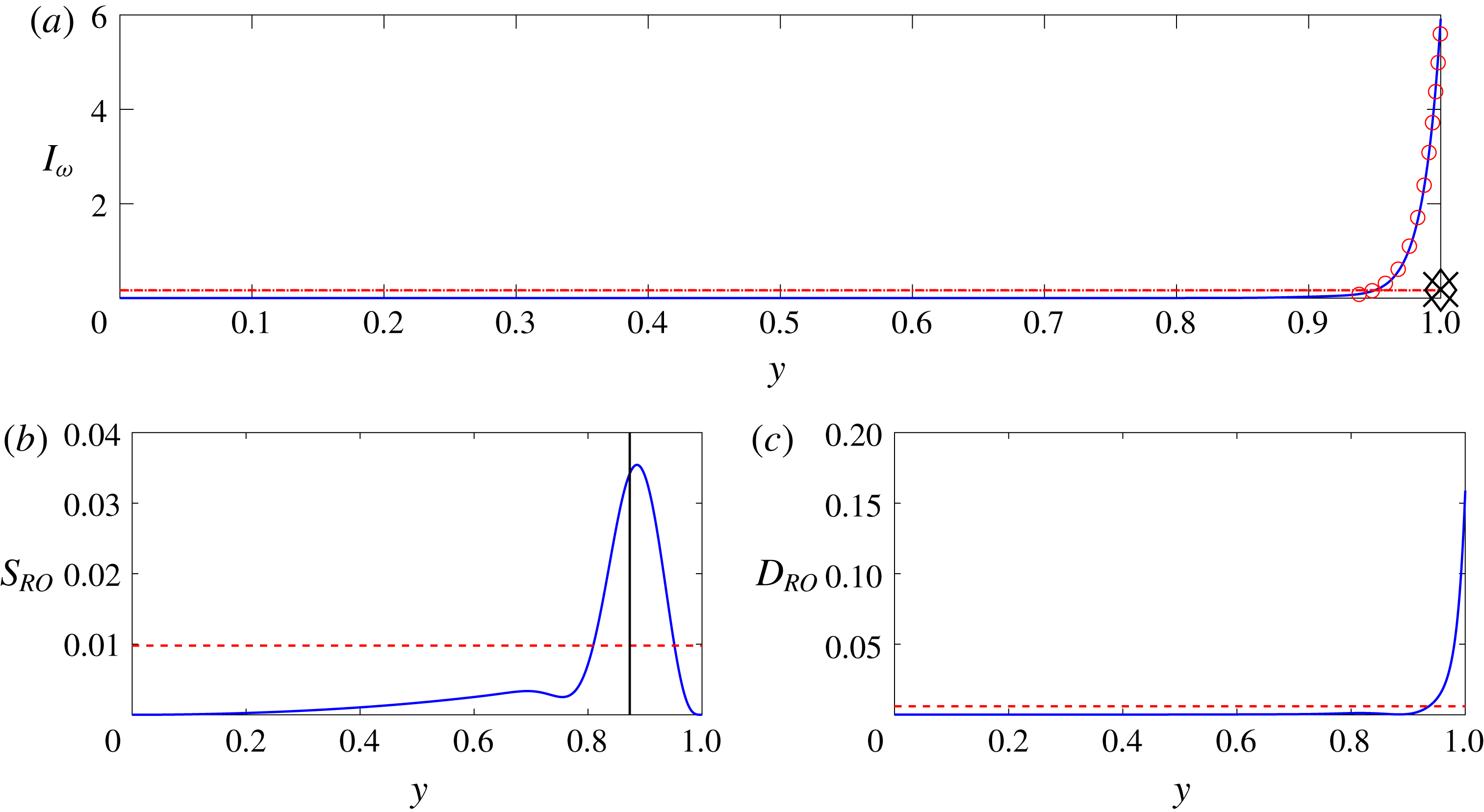
Production and damping of the perturbation’s enstrophy and kinetic energy for the unstable mode of viscous planar Poiseuille flow under
 $\unicode[STIX]{x1D6FC}=1$
,
 $R=10^{4}$
with
 $c=0.2375+0.0037i$
: (a) the solid curve represents the vorticity damping function
 $I_{\unicode[STIX]{x1D714}}$
over
 $0\leqslant y\leqslant 1$
, the dashed horizontal line represents the integral of
 $I_{\unicode[STIX]{x1D714}}$
over
 $-1\leqslant y\leqslant 1$
, which is equal to
 $p_{I}=0.1657$
, and the diamond at
 $y=1$
stands for the vorticity production quantity
 $p_{B}=0.1694$
. In addition, the circles represent
 $I_{\unicode[STIX]{x1D714}_{bl}}$
due to the boundary layer solution (4.8) in a vicinity of
 $y=1$
, the dotted horizontal line represents the vorticity damping resultant near
 $y=\pm 1$
, namely
 $p_{I}^{\ast }=0.1640$
, and the cross label at
 $y=1$
stands for the vorticity production quantity due to wall boundary layers near
 $y=\pm 1$
, namely
 $p_{B_{bl}}=0.1820$
; (b) the solid curve represents the Reynolds stress function
 $S_{RO}(\,y)$
over
 $0\leqslant y\leqslant 1$
, the dashed horizontal line represents the integral of
 $S_{RO}$
over
 $-1\leqslant y\leqslant 1$
, which is equal to
 $S=0.0098$
, and the solid vertical line stands for the critical point
 $y_{c}=\sqrt{1-c_{r}}=0.8732$
; (c) the solid curve represents the kinetic energy damping function
 $D_{RO}(\,y)$
over
 $0\leqslant y\leqslant 1$
, the dashed horizontal line represents the integral of
 $D_{RO}$
over
 $-1\leqslant y\leqslant 1$
, which is equal to
 $D=0.0061$
.

The unique unstable mode has associated
 $c=0.2375+0.0037i$
. As shown in figure 4(a), the vorticity production term
 $B_{\unicode[STIX]{x1D714}}$
at the walls gives rise to
 $p_{B}=0.1694$
(the diamond label). Also, the damping of the vorticity is primarily sustained in a neighbourhood of
 $y=\pm 1$
, with an accumulated value
 $p_{I}=0.1657$
(the dashed line). The overall contribution of the perturbation’s vorticity is measured by
 $c_{i}=p_{B}-p_{I}=0.0037$
, which is only a small portion of
 $p_{B}$
. Specifically, we find that
 $c_{i}/p_{B}\approx 2.18\,\%$
.
Identity (4.5a
) and figure 4(a) suggest an interconnection between values of
 $p_{B}$
and
 $p_{I}$
for this unstable mode. That is,
 $p_{B}$
is strongly related to the gradient of the perturbation’s vorticity across the walls, which in turn quantifies the steepness of the vorticity damping function
 $I_{\unicode[STIX]{x1D714}}$
(the solid curve) in a vicinity of
 $y=\pm 1$
, and hence it affects the area under the
 $I_{\unicode[STIX]{x1D714}}$
curve near the walls, namely the value of
 $p_{I}$
. Such interconnection between
 $p_{B}$
and
 $p_{I}$
near the wall boundaries explains the small difference in their magnitudes. Moreover, it implies that the wall boundary layer effect had played a dominant role in sustaining the growth of the mode.
To validate our hypothesis regarding the wall boundary layer effect, we define
 $$\begin{eqnarray}p_{I}^{\ast }:=\int _{\pm [0.9,1]}I_{\unicode[STIX]{x1D714}}(\,y)\,\text{d}y.\end{eqnarray}$$
Also, we adopt the following wall boundary layer solution that holds for a vicinity of
 $y=\pm 1$
(see (27.5) on p. 167 of Drazin & Reid Reference Drazin and Reid2004):
 $$\begin{eqnarray}\unicode[STIX]{x1D719}_{bl}(\,y)\sim \exp \left[(\pm y-1)\sqrt{\unicode[STIX]{x1D6FC}Rc}\text{e}^{-\unicode[STIX]{x03C0}\text{i}/4}\right],\quad y\sim \pm 1\end{eqnarray}$$
and denote its associated quantities by the aforementioned symbols with a subscript
 $bl$
.
The
 $I_{\unicode[STIX]{x1D714}_{bl}}$
function is shown in figure 4(a) as circles over
 $y\in [0.9,1]$
, from which we observe an evident agreement between
 $I_{\unicode[STIX]{x1D714}}$
and
 $I_{\unicode[STIX]{x1D714}_{bl}}$
. Moreover, the value
 $p_{I}^{\ast }=0.1640$
(the dotted line) is close to the value
 $p_{I}=0.1657$
(the dashed line), and the value
 $p_{B_{bl}}=0.1820$
(the cross label) is close to the value
 $p_{B}=0.1694$
(the diamond label). The growth of the mode is thus predominantly sustained by the wall boundary layer.
Figure 4(b) represents the contribution to the growth rate due to the Reynolds stress function
 $S_{RO}$
that appears in (4.6c
). It exhibits two contrasting features in comparison to the vorticity-based quantity
 $B_{\unicode[STIX]{x1D714}}$
. First, the shape of the
 $S_{RO}$
function indicates that the production of the perturbation’s kinetic energy is spread out over the entire range of the fluid domain, with its peak value reached slightly to the right of the critical layer
 $y_{c}=\sqrt{1-c_{r}}=0.8732$
(the solid vertical line). This observation was also made by Drazin (see Drazin & Reid Reference Drazin and Reid2004, p. 223). Secondly, there is zero energy production at the wall boundary. The overall energy production is quantified by the area under the
 $S_{RO}$
curve, which is
 $S=0.0098$
(the dashed line). On the other hand, as shown by figure 4(c), the energy damping function
 $D_{RO}$
demonstrates a similar trend to that of the vorticity damping function
 $I_{\unicode[STIX]{x1D714}}$
, with an integrated value
 $D=0.0061$
(the dashed line).
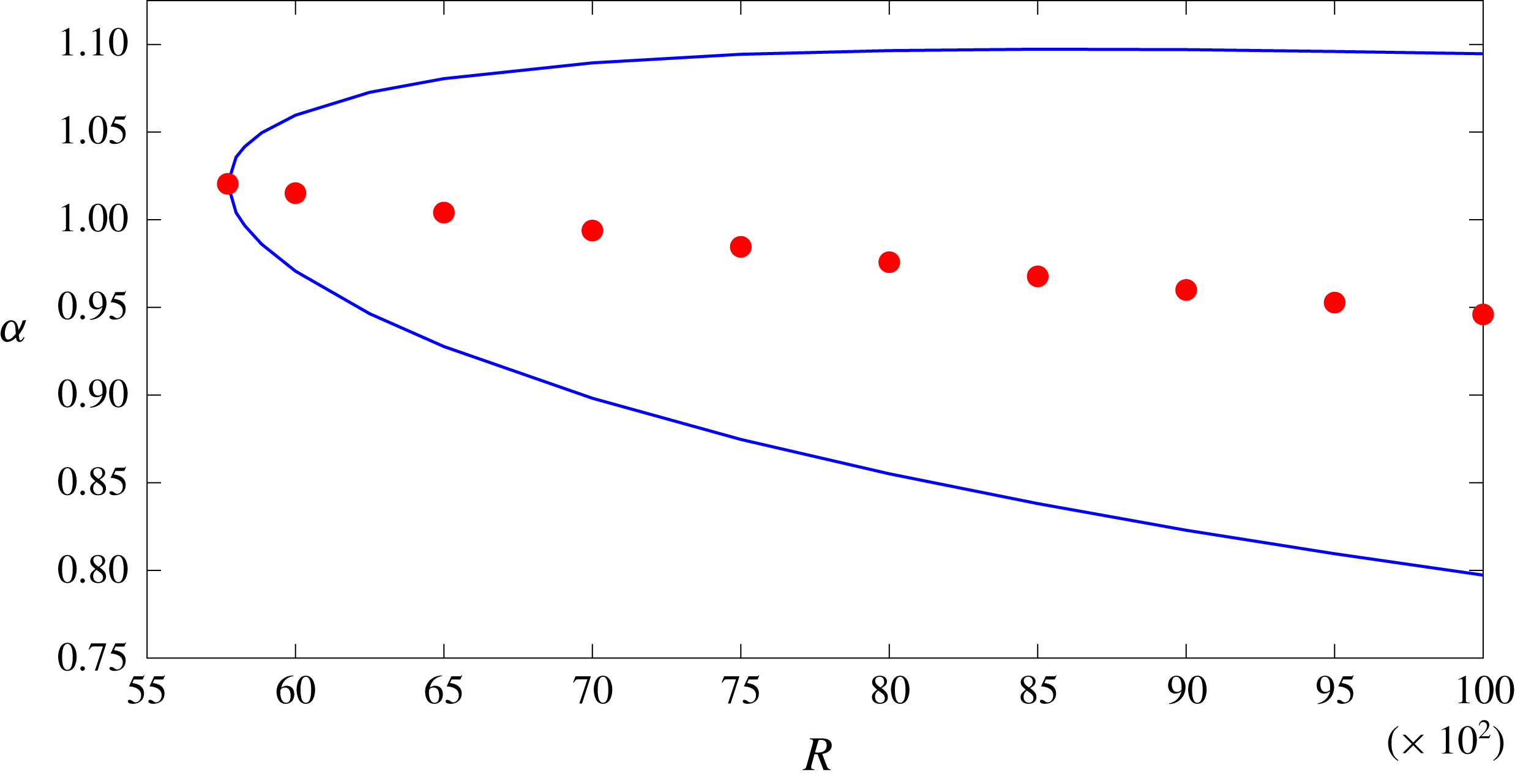
As a validation of the observations made above for an unstable mode, we selected ten further unstable modes with
 $R$
ranges from 5772 (the critical Reynolds number corresponding to the onset of linear instability) to 10 000. These modes are located halfway along the stability boundaries in the
 $(\unicode[STIX]{x1D6FC},R)$
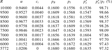
plane, as shown by the dots in figure 5. The stability parameters associated with these modes are presented in table 1.
The marginal linear stability boundary (the solid curve) of planar Poiseuille flow. The region enclosed by the stability boundary consists of unstable modes. Stability parameters associated with the pre-selected modes (solid dots) are presented in table 1.

Stability parameters of pre-seleced unstable modes shown in figure 5.

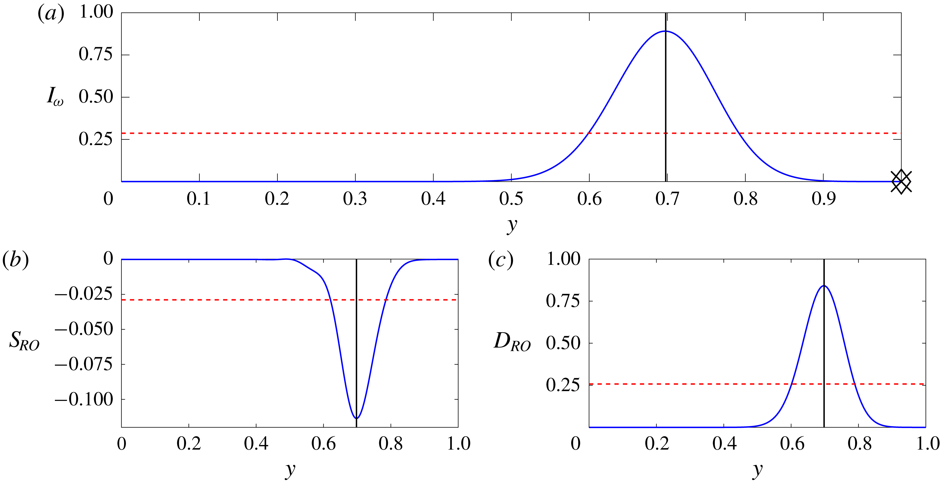
To demonstrate the stability mechanism for this flow, we consider another symmetric (even) mode under the same set of parameters but with
 $c=0.5129-0.2866i$
. The corresponding plots are shown in figure 6, with the critical point
 $y_{c}=0.6979$
shown as a solid vertical line in each plot. It is evident that the Reynolds stress
 $S_{RO}$
and the energy damping function
 $D_{RO}$
are both almost symmetrically distributed about the critical point, as is the vorticity damping function
 $I_{\unicode[STIX]{x1D714}}$
. The corresponding integrated quantities are
 $p_{I}=0.2866$
,
 $S=-0.0289$
and
 $D=0.2578$
, respectively (dashed lines).
Production and damping of the perturbation’s enstrophy and kinetic energy for the stable symmetric mode of viscous planar Poiseuille flow under
 $\unicode[STIX]{x1D6FC}=1$
,
 $R=10^{4}$
with
 $c=0.5129-0.2866i$
. In all plots, the solid vertical line stands for the critical point
 $y_{c}=0.6979$
: (a) the solid curve represents the vorticity damping function
 $I_{\unicode[STIX]{x1D714}}$
over
 $0\leqslant y\leqslant 1$
, the dashed horizontal line represents the integral of
 $I_{\unicode[STIX]{x1D714}}$
over
 $-1\leqslant y\leqslant 1$
, which is equal to
 $p_{I}=0.2866$
, the diamond at
 $y=1$
stands for the vorticity production quantity
 $p_{B}=-1.014\times 10^{-7}$
, and the cross label at
 $y=1$
stands for the vorticity production quantity due to wall boundary layers, namely
 $p_{B_{bl}}=-1.109\times 10^{-7}$
; (b) the solid curve represents the Reynolds stress function
 $S_{RO}$
over
 $0\leqslant y\leqslant 1$
, the dashed horizontal line represents the integral of
 $S_{RO}$
over
 $-1\leqslant y\leqslant 1$
, namely
 $S=-0.0289$
; (c) the solid curve represents the kinetic energy damping function
 $D_{RO}(\,y)$
over
 $0\leqslant y\leqslant 1$
, the dashed horizontal line represents the integral of
 $D_{RO}$
over
 $-1\leqslant y\leqslant 1$
, namely
 $D=0.2578$
.

The vorticity production quantities of this mode are
 $p_{B}=-1.014\times 10^{-7}$
(the diamond label) and
 $p_{B_{bl}}=-1.109\times 10^{-7}$
(the cross label), which are both negligible; hence it exhibits little vorticity production at the walls. Also, the vorticity damping function
 $I_{\unicode[STIX]{x1D714}}$
is accumulated over the subinterval
 $[0.48,0.9]$
, outside which the value of
 $I_{\unicode[STIX]{x1D714}}$
is relatively negligible. This indicates that there is also little damping of the perturbation’s vorticity in a vicinity of
 $y=\pm 1$
. These phenomena are consistent with the aforementioned interconnection between
 $p_{B}$
and the portion of
 $p_{I}$
near the walls.
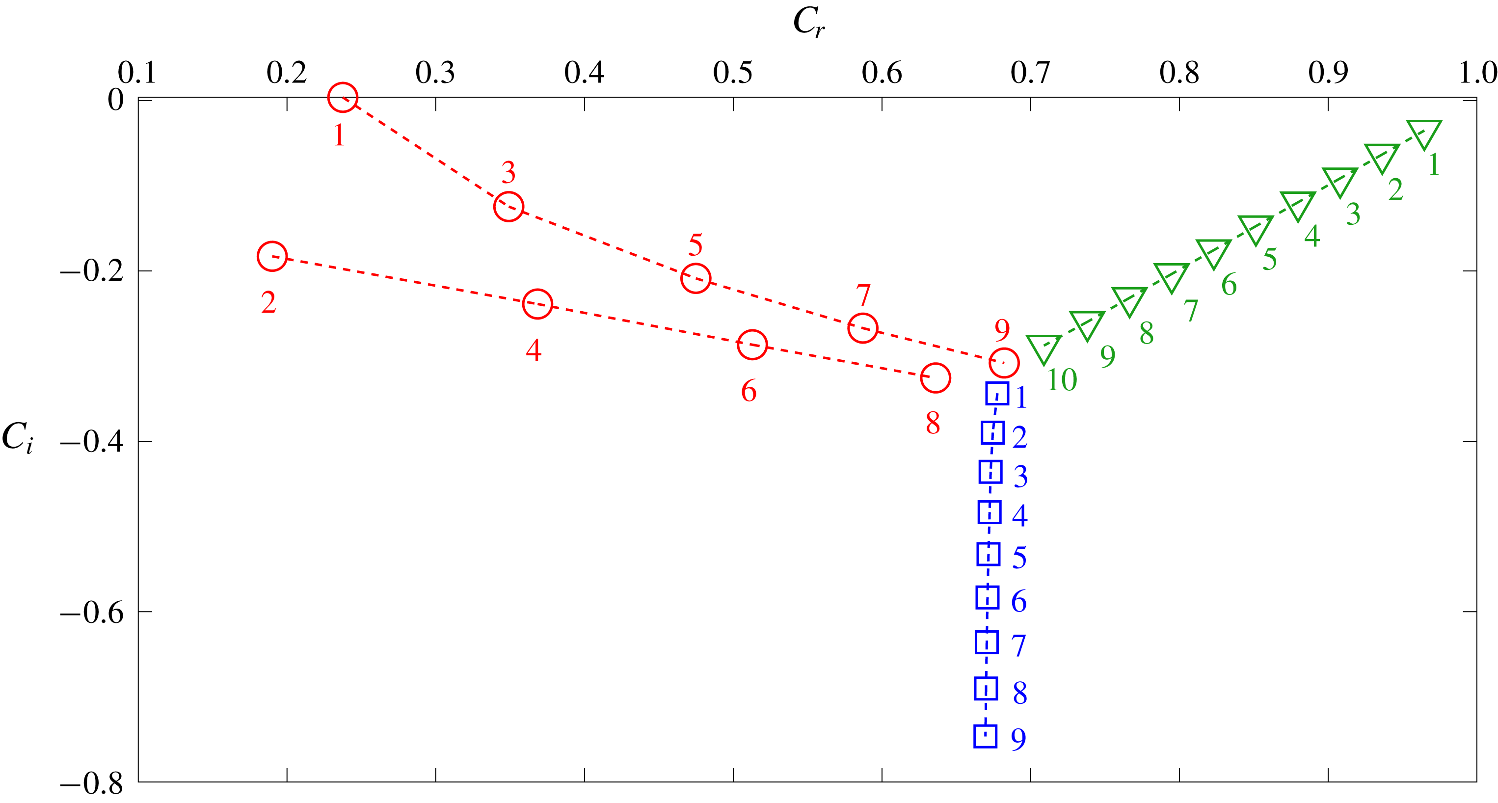
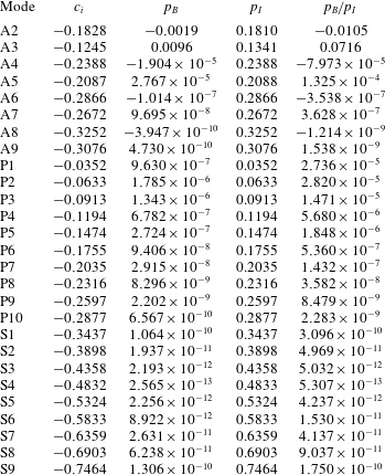
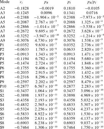
Similar observations have been made by other authors through carefully examining other stable symmetric modes under the prescribed parameters. See a summary of these modes in figure 7 and table 2. Specifically, we observe in those stable modes that the damping of vorticity is accumulated in a neighbourhood of their corresponding critical points away from the boundary layers, and there is considerably less vorticity production at the walls. These are different from the observations made for the boundary layer dominant case, where production and damping of vorticity are both sustained with similar magnitudes within the boundary layer. In other words, from the perspective of vorticity, a sufficiently strong wall boundary layer effect is necessary for the onset of instability.
The distribution of eigenvalues of symmetric modes for viscous planar Poiseuille flow at
 $\unicode[STIX]{x1D6FC}=1$
and
 $R=10\,000$
. The circles, wedges and squares stand for modes of the A family, P family and S family, respectively (notation adopted by Mack (Reference Mack1976)). Stability parameters associated with the stable modes are presented in table 2.

Stability parameters of the symmetric stable modes summarized in figure 7.
Remark.
The above study on shear flow stability was based on (3.11) established under the no-slip wall boundary condition. This preliminary study provides a different view from the one based on the classical Reynolds–Orr kinetic energy equation. In particular, the current approach has its root in the vorticity motion of the flow. As was remarked by Küchemann (Reference Küchemann1965), vortices are ‘the sinews and muscles of fluid motions’. Indeed, by pursuing the ‘sinews’, one would be able to ascribe precisely the unique production source of the perturbation’s enstrophy to the walls, over which the flow is ‘rubbed’ due to the enforced no-slip wall boundary condition.
It is evident that the internal flow always makes a direct contribution to the perturbation’s enstrophy only as a damping constituent, which was quantified by the term
 $-p_{I}$
in (4.5c
). Specifically, the critical layer is a primary source of damping of the perturbation’s enstrophy at high Reynolds numbers. The relatively large magnitude of the damping source at high Reynolds numbers is a consequence of the singularity that forms at the critical layer in the inviscid limit of the flow.
In summary, the current study shows a natural interconnection between viscous and inviscid flow stability mechanisms for non-inflectional shear flows. The viscous and inviscid stability mechanisms are hence two sides of the same coin. Also, formulations based on enstrophy and kinetic energy reveal different faces of the same physical reality – they enrich and complement each other.
4.2 A control scheme for the wall boundary’s vorticity for viscous planar Poiseuille flow
Recall from Example 3.2 that the wall condition
 $(\widetilde{u},\widetilde{\unicode[STIX]{x1D714}})=(0,0)$
would imply global nonlinear stability for the base planar Poiseuille flow. It is also clear that the same is true for the free-slip wall condition, namely
 $(\widetilde{v},\widetilde{\unicode[STIX]{x1D714}})=(0,0)$
.
We propose the following wall boundary control scheme, in which
 $l_{s}\in [0,1]$
is the control parameter:
 $$\begin{eqnarray}\left.\begin{array}{@{}c@{}}\widehat{v}(\pm 1)=0,\\ (1-l_{s})\widehat{u}(\pm 1)\mp l_{s}\widehat{\unicode[STIX]{x1D714}}(\pm 1)=0.\end{array}\right\}\end{eqnarray}$$
This control scheme can be regarded as an extension (or a relaxation) of the free-slip wall condition
 $(\widetilde{v},\widetilde{\unicode[STIX]{x1D714}})=(0,0)$
that corresponds to the special case when
 $l_{s}=1$
. On the other hand, the case with
 $l_{s}=0$
corresponds to the uncontrolled unstable base flow under the no-slip wall condition. The control scheme is aimed at seeking an intermediate value of the control parameter for which the base Poiseuille flow under the wall conditions (4.9) becomes stable. Note that for each
 $l_{s}$
, the vorticity wall condition in (4.9) can be realized by matching the velocity
 $\widetilde{u}(x,\pm 1,t)$
(e.g. through an actuator in engineering practice) according to the instantly measured
 $\unicode[STIX]{x2202}\widetilde{u}/\unicode[STIX]{x2202}y$
(
 $=-\widetilde{\unicode[STIX]{x1D714}}$
).
To further understand the qualitative behaviour of the control scheme, we conduct a linear stability analysis of the base Poiseuille flow under wall conditions (4.9).
Note that in accordance with Theorem 3.2 (in the limit as
 $V\rightarrow 0$
) or Theorem 3.3, the vorticity-based identity (4.5a
) is still valid under the proposed wall boundary conditions due to
 $\widetilde{v}=0$
at the walls, but the Reynolds–Orr kinetic energy equation (4.6a
) is not valid for
 $l_{s}\neq 0$
.
As a test for the above wall vorticity control scheme, we consider the viscous planar Poiseuille flow studied in § 4.1 with
 $\unicode[STIX]{x1D6FC}=1$
,
 $R=10\,000$
. Equation (4.2) imposed under (4.9) is numerically solved for
 $0\leqslant l_{s}\leqslant 1$
by using the standard Chebyshev collocation method (Boyd Reference Boyd2000). Note that we are looking for the mode corresponding to the largest growth rate for each
 $l_{s}$
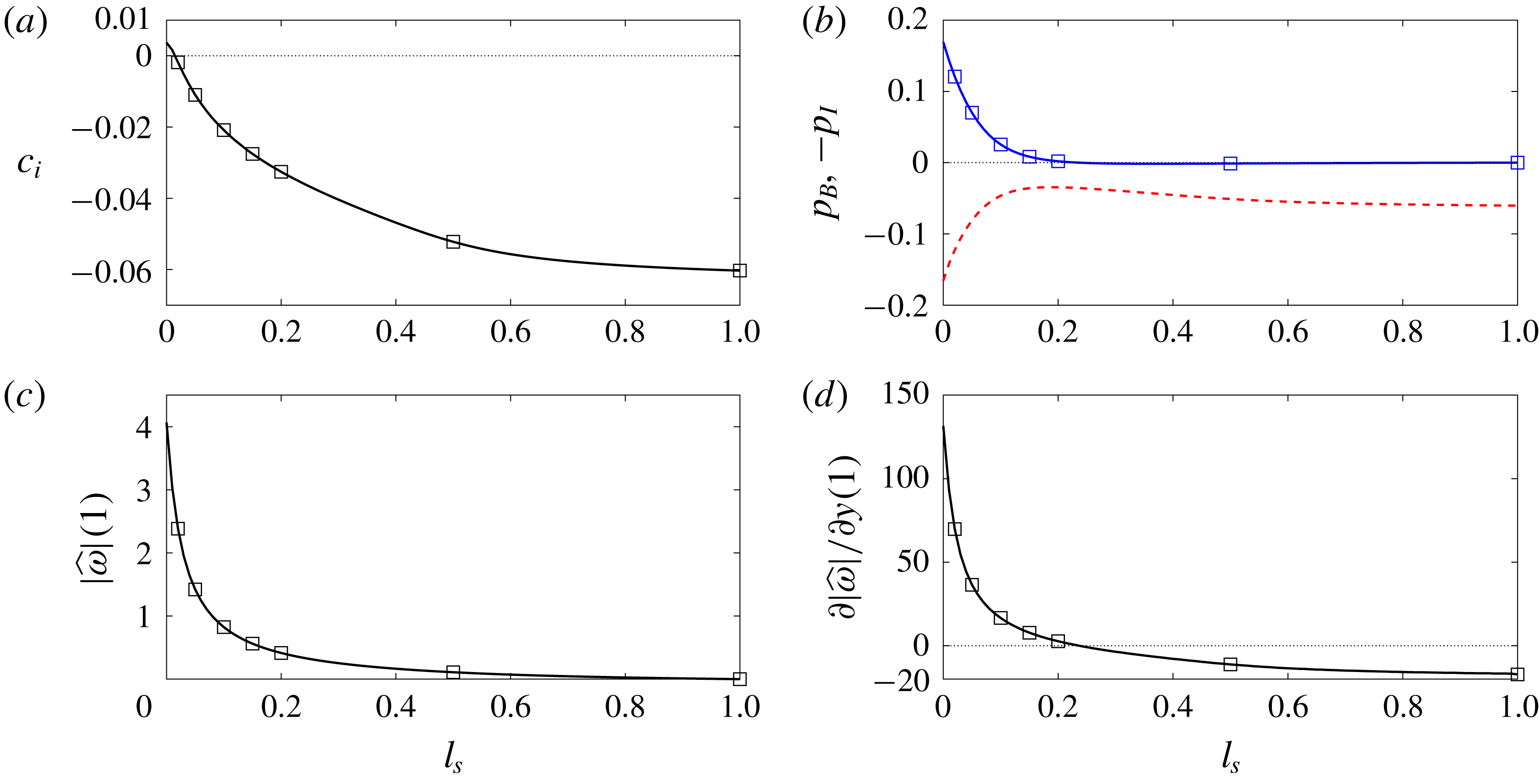
. Results are summarized in figure 8. Figure 8(a) shows that the growth rate
 $c_{i}$
(the solid curve) monotonically decreases as
 $l_{s}$
increases and the flow is stabilized at
 $l_{s}=1.481\,\%$
. Such a rapid decreasing trend of
 $c_{i}$
with respect to
 $l_{s}$
indicates that the stability of the flow is sensitive to the proposed control scheme. Besides, the successively added vorticity component in (4.9), namely
 $\mp l_{s}\widehat{\unicode[STIX]{x1D714}}^{\prime \prime }(\pm 1)$
, would always shift the flow into a more stable state.
The largest growth rate
 $c_{i}$
and its constituents as functions of the control parameter
 $l_{s}$
for viscous planar Poiseuille flow at
 $\unicode[STIX]{x1D6FC}=1$
,
 $R=10^{4}$
. Pre-selected points for further display are marked by squares, and the horizontal dotted lines are the zero reference lines: (a) growth rate
 $c_{i}$
as a function of
 $l_{s}$
; (b) the two constituents
 $p_{B}$
(solid curve) and
 $-p_{I}$
(dashed curve) as functions of
 $l_{s}$
based on (4.5a
); (c) the modulus of
 $\widehat{\unicode[STIX]{x1D714}}$
at
 $y=1$
as a function of
 $l_{s}$
; (d) the normal derivative of
 $|\widehat{\unicode[STIX]{x1D714}}|$
at
 $y=1$
as a function of
 $l_{s}$
.

To further illustrate the change in flow stability with respect to the control parameter, we present in figure 8(b) the constituents
 $p_{B}$
and
 $p_{I}$
of the growth rate as a function of
 $l_{s}$
. Clearly, the constituent
 $p_{B}$
(the solid curve) strictly decreases over
 $0\leqslant l_{s}\leqslant 20\,\%$
, with zero reached at about
 $l_{s}=20\,\%$
; thereafter it remains approximately a constant that is slightly below zero until
 $l_{s}$
reaches 100 %. Moreover, figure 8(c,d) indicates that the decrease in the wall boundary’s vorticity would also lead to a decrease in its normal derivative across the walls. However, it is evident that the magnitude of
 $\widehat{\unicode[STIX]{x1D714}}(1)$
is always much less than that of
 $(\unicode[STIX]{x2202}\widehat{\unicode[STIX]{x1D714}}/\unicode[STIX]{x2202}y)(1)$
at each given
 $l_{s}$
. Thus, the test suggests that the instability of the flow is primarily restrained by the amount of perturbation’s vorticity at the walls, namely
 $\widehat{\unicode[STIX]{x1D714}}(\pm 1)$
itself, but not its normal derivative across the walls.
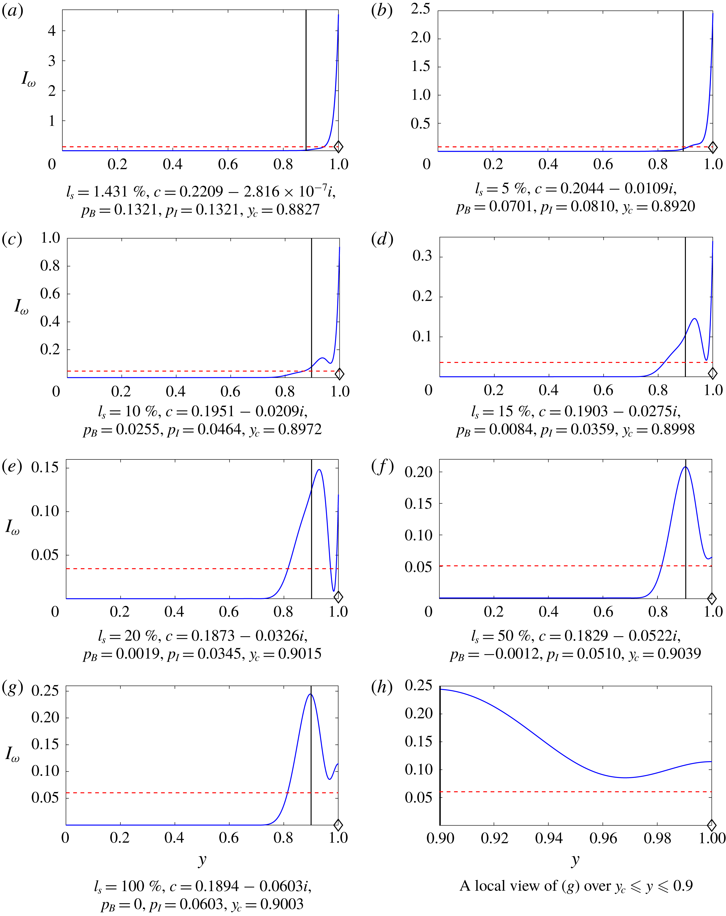
Figure 9 displays the vorticity damping functions
 $I_{\unicode[STIX]{x1D714}}$
corresponding to a set of pre-selected
 $l_{s}$
. The plots reveal two subregions in
 $0\leqslant y\leqslant 1$
over which
 $I_{\unicode[STIX]{x1D714}}$
takes significantly non-zero values. Specifically, they are the inner bump region that has a peak value which is slightly beyond the critical point
 $y=y_{c}$
, and an outer region which is adjacent to the inner region, that culminates at
 $y=1$
.
Controlled cases for viscous planar Poiseuille flow under
 $\unicode[STIX]{x1D6FC}=1$
,
 $R=10^{4}$
with pre-selected control parameters
 $l_{s}$
: the solid curve in each subfigure represents the vorticity damping function
 $I_{\unicode[STIX]{x1D714}}(\,y)$
, the dashed horizontal line represents the value of
 $p_{I}$
, the diamond at
 $y=1$
stands for the value of
 $p_{B}$
and the vertical line stands for the critical point
 $y=y_{c}$
.

As one may observe from the plots in figure 9,
 $I_{\unicode[STIX]{x1D714}}^{\prime }(1)$
and
 $p_{B}$
both decrease as
 $l_{s}$
increases. In particular, for the case
 $l_{s}=1$
, we see from figure 9(h) that
 $I_{\unicode[STIX]{x1D714}}^{\prime }(1)=0$
. This validates the interconnection between
 $p_{B}$
and the steepness of
 $I_{\unicode[STIX]{x1D714}}$
at the walls, which was concluded in § 4.1. In addition, the inner region bulges as
 $l_{s}$
increases, with its peak value gradually exceeding
 $I_{\unicode[STIX]{x1D714}}(1)$
as
 $l_{s}$
approaches 20 %, after which the inner region significantly ‘overwhelms’ the outer region in terms of its contribution to
 $I_{\unicode[STIX]{x1D714}}$
. The overwhelming of the outer region by the inner is reflected through the plot of
 $-p_{I}$
versus
 $l_{s}$
in figure 8(b) (the dashed curve), in which we observe an initial decrease in
 $p_{I}$
due to the rapid decrease in the steepness of
 $I_{\unicode[STIX]{x1D714}}$
at
 $y=1$
, that lasts over
 $0<l_{s}<20\,\%$
, while
 $p_{I}$
increases thereafter due to accelerated bulging of the inner region and diminishing of the outer region.
These observations validate the conclusions drawn based on the study of the uncontrolled flow in § 4.1, that the presence of a steep outer region of
 $I_{\unicode[STIX]{x1D714}}$
is necessary for the production of perturbation’s enstrophy, and hence it promotes instability of the flow. On the other hand, the presence of
 $I_{\unicode[STIX]{x1D714}}$
with a significantly bulged inner region and a relatively diminished outer region indicates a much more stabilized flow.
5 Summary and conclusions
A viscous extension of Arnold’s theory to planar non-inflectional shear flows was developed. The extension in the form of the viscous Arnold’s identity (Theorem 3.1) complements Arnold’s stability theory on inviscid shear flows subject to arbitrary two-dimensional perturbations. The viscous Arnold’s identity contains viscous terms only. It led to a number of perturbation’s enstrophy identities that are valid for a variety of flow motions under various wall boundary conditions.
As a first application of our viscous Arnold’s identity, we found an alternative derivation of the classical perturbation’s enstrophy identity under linear dynamics that was established earlier by Synge (Reference Synge1938) and Fraternale et al. (Reference Fraternale, Domenicale, Staffilani and Tordella2018). The enstrophy identity consists of a boundary component at the walls and a damping component in the fluid bulk, with the presence of viscosity in both components being a feature that is consistent with the viscous Arnold’s identity.
We have established a new weighted perturbation’s enstrophy identity in the form of Theorem 3.2 based on the viscous Arnold’s identity, which is valid for non-inflectional streamwise translation-invariant base laminar states under linear dynamics. The weighted identity holds under two classes of relaxed wall boundary conditions.
We showed that the perturbation’s enstrophy identity for strictly parallel base states is preserved under global nonlinear dynamics. This is a direct consequence of the fully nonlinear viscous Arnold’s identity. Furthermore, we examined the validity of the perturbation’s enstrophy identity under more general wall boundary conditions than the no-slip condition. The results are summarized as Theorem 3.3.
As a case study, the enstrophy identity under global nonlinear dynamics imposed with the free-slip (zero disturbance’s vorticity) wall condition was applied to viscous planar Poiseuille flow, thereby unconditional global stability for the flow was rigorously deduced. The corresponding decay rate of a vorticity disturbance was estimated through Example 3.2. The case study illustrates a novel stabilization mechanism that inhibits the growth of any two-dimensional disturbance, and implementation of the mechanism may lead to effective flow control methodologies.
To explore the physical mechanisms of linear instability/stability from the perspective of enstrophy, we carried out a preliminary study in § 4 for viscous planar Poiseuille flow. Distributions of disturbance’s enstrophy at/between the walls were investigated within the classical normal modal framework. We found that the critical layer is always a direct source of damping in disturbance’s enstrophy for all the cases computed.
We observed a subtle interaction between a critical layer and its adjacent boundary layer, which determines the stability nature of the flow. We remark that the underlying inviscid mechanism also plays a role in the interaction between the two layers, although it is not explicitly included the viscous enstrophy identity.
As an implementation of the relaxed wall conditions imposed for the enstrophy identity, we proposed a control scheme for the wall boundary’s vorticity disturbance. The control scheme transitions the wall settings from the no-slip condition to the free-slip condition. The linearly unstable viscous planar Poiseuille flow originally imposed under the no-slip wall condition becomes stabilized after addition of about 2 % of the free-slip wall effect.
It should be remarked that the current study is limited to two-dimensional disturbances. On the other hand, it is well known that flow three-dimensionality can develop in two-dimensional boundary layers relatively fast (see Kachanov Reference Kachanov1994). Thus, a three-dimensional disturbance may cause a linearly stable (against two-dimensional disturbances) laminar boundary layer to undergo an intricate transition into a turbulent state. The effectiveness of the control method proposed in the current study, therefore, must be re-assessed in future studies for cases where three-dimensional disturbances arise.
Appendix A. Derivation of Theorem 3.1
The total kinetic energy of a flow is
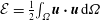 ${\mathcal{E}}=\frac{1}{2}\int _{\unicode[STIX]{x1D6FA}}\boldsymbol{u}\boldsymbol{\cdot }\boldsymbol{u}\,\text{d}\unicode[STIX]{x1D6FA}$
. In accordance with (2.5), we have the following identity:
 $$\begin{eqnarray}\displaystyle & & \displaystyle \frac{\text{d}{\mathcal{E}}}{\text{d}t}+\frac{1}{2}\int _{\unicode[STIX]{x2202}\unicode[STIX]{x1D6FA}}|\boldsymbol{u}|^{2}\boldsymbol{u}\boldsymbol{\cdot }\text{d}\boldsymbol{S}+\int _{\unicode[STIX]{x2202}\unicode[STIX]{x1D6FA}}p\boldsymbol{u}\boldsymbol{\cdot }\text{d}\boldsymbol{S}\nonumber\\ \displaystyle & & \displaystyle \quad =\frac{1}{R}\left(\int _{\unicode[STIX]{x2202}\unicode[STIX]{x1D6FA}}u\unicode[STIX]{x1D735}u\boldsymbol{\cdot }\text{d}\boldsymbol{S}+\int _{\unicode[STIX]{x2202}\unicode[STIX]{x1D6FA}}v\unicode[STIX]{x1D735}v\boldsymbol{\cdot }\text{d}\boldsymbol{S}-\int _{\unicode[STIX]{x1D6FA}}|\unicode[STIX]{x1D735}\boldsymbol{u}|^{2}\,\text{d}\unicode[STIX]{x1D6FA}\right).\end{eqnarray}$$
Recall that
 ${\mathcal{E}}_{0}=\frac{1}{2}\int _{\unicode[STIX]{x1D6FA}}U_{0}^{2}\,\text{d}\unicode[STIX]{x1D6FA}$
and
 $\widetilde{{\mathcal{E}}}={\mathcal{E}}-{\mathcal{E}}_{0}$
. Substituting (2.9) into (A 1), and using (2.8), (2.10), (2.12) together with streamwise periodicity we obtain the following:
 $$\begin{eqnarray}\displaystyle \frac{\text{d}\widetilde{{\mathcal{E}}}}{\text{d}t} & = & \displaystyle \frac{\text{d}{\mathcal{E}}}{\text{d}t}-\frac{\text{d}{\mathcal{E}}_{0}}{\text{d}t}\nonumber\\ \displaystyle & = & \displaystyle -\int _{-1}^{1}[p_{0}(L)-p_{0}(-L)]\widetilde{u}(L,y)\,\text{d}y-\int _{\unicode[STIX]{x1D6FA}}U_{0}\frac{\unicode[STIX]{x2202}\widetilde{p}}{\unicode[STIX]{x2202}x}\,\text{d}\unicode[STIX]{x1D6FA}\nonumber\\ \displaystyle & & \displaystyle +\,\frac{1}{R}\int _{-L}^{L}\left[U_{0}(1)\frac{\unicode[STIX]{x2202}\widetilde{u}}{\unicode[STIX]{x2202}y}(x,1)-U_{0}(-1)\frac{\unicode[STIX]{x2202}\widetilde{u}}{\unicode[STIX]{x2202}y}(x,-1)\right]\text{d}x\nonumber\\ \displaystyle & & \displaystyle -\,\frac{1}{R}\int _{\unicode[STIX]{x1D6FA}}|\unicode[STIX]{x1D735}\widetilde{u}|^{2}+|\unicode[STIX]{x1D735}\widetilde{v}|^{2}+2U_{0}^{\prime }\frac{\unicode[STIX]{x2202}\widetilde{u}}{\unicode[STIX]{x2202}y}\,\text{d}\unicode[STIX]{x1D6FA}\nonumber\\ \displaystyle & = & \displaystyle -\int _{\unicode[STIX]{x1D6FA}}U_{0}\frac{\unicode[STIX]{x2202}\widetilde{p}}{\unicode[STIX]{x2202}x}\,\text{d}\unicode[STIX]{x1D6FA}+\frac{1}{R}\int _{\unicode[STIX]{x1D6FA}}U_{0}\frac{\unicode[STIX]{x2202}^{2}\widetilde{u}}{\unicode[STIX]{x2202}y^{2}}+U_{0}^{\prime }\frac{\unicode[STIX]{x2202}\widetilde{u}}{\unicode[STIX]{x2202}y}\,\text{d}\unicode[STIX]{x1D6FA}-\frac{1}{R}\int _{\unicode[STIX]{x1D6FA}}|\unicode[STIX]{x1D735}\widetilde{u}|^{2}+|\unicode[STIX]{x1D735}\widetilde{v}|^{2}+2U_{0}^{\prime }\frac{\unicode[STIX]{x2202}\widetilde{u}}{\unicode[STIX]{x2202}y}\,\text{d}\unicode[STIX]{x1D6FA}\nonumber\\ \displaystyle & = & \displaystyle -\int _{\unicode[STIX]{x1D6FA}}U_{0}\frac{\unicode[STIX]{x2202}\widetilde{p}}{\unicode[STIX]{x2202}x}\,\text{d}\unicode[STIX]{x1D6FA}+\frac{1}{R}\int _{\unicode[STIX]{x1D6FA}}U_{0}\frac{\unicode[STIX]{x2202}^{2}\widetilde{u}}{\unicode[STIX]{x2202}y^{2}}\,\text{d}\unicode[STIX]{x1D6FA}+\frac{1}{R}\int _{\unicode[STIX]{x1D6FA}}U_{0}^{\prime \prime }\widetilde{u}\,\text{d}\unicode[STIX]{x1D6FA}-\frac{1}{R}\int _{\unicode[STIX]{x1D6FA}}|\unicode[STIX]{x1D735}\widetilde{u}|^{2}+|\unicode[STIX]{x1D735}\widetilde{v}|^{2}\,\text{d}\unicode[STIX]{x1D6FA}\nonumber\\ \displaystyle & = & \displaystyle -\int _{\unicode[STIX]{x1D6FA}}U_{0}\frac{\unicode[STIX]{x2202}\widetilde{p}}{\unicode[STIX]{x2202}x}\,\text{d}\unicode[STIX]{x1D6FA}+\frac{1}{R}\int _{\unicode[STIX]{x1D6FA}}U_{0}\frac{\unicode[STIX]{x2202}^{2}\widetilde{u}}{\unicode[STIX]{x2202}y^{2}}\,\text{d}\unicode[STIX]{x1D6FA}-\frac{1}{R}\int _{\unicode[STIX]{x1D6FA}}|\unicode[STIX]{x1D735}\widetilde{u}|^{2}+|\unicode[STIX]{x1D735}\widetilde{v}|^{2}\,\text{d}\unicode[STIX]{x1D6FA},\end{eqnarray}$$
in which we have used the fact that
 $\int _{\unicode[STIX]{x1D6FA}}\widetilde{u}\,\text{d}\unicode[STIX]{x1D6FA}=\int _{\unicode[STIX]{x1D6FA}}(\unicode[STIX]{x2202}\widetilde{\unicode[STIX]{x1D713}}/\unicode[STIX]{x2202}y)\,\text{d}\unicode[STIX]{x1D6FA}=\int _{-L}^{L}[\widetilde{\unicode[STIX]{x1D713}}]_{y=-1}^{y=1}\,\text{d}x=0$
.
The associated Casimir function was defined to be
 ${\mathcal{C}}_{s}=\int _{\unicode[STIX]{x1D6FA}}F(\unicode[STIX]{x1D714})\,\text{d}\unicode[STIX]{x1D6FA}$
. Recall that
 ${\mathcal{C}}_{s0}=\int _{\unicode[STIX]{x1D6FA}}F(\unicode[STIX]{x1D714}_{0})\,\text{d}\unicode[STIX]{x1D6FA}$
and
 $\widetilde{{\mathcal{C}}}_{s}={\mathcal{C}}_{s}-{\mathcal{C}}_{s0}$
. In accordance with (2.11), the streamwise periodicity of
 $\unicode[STIX]{x1D713}$
and
 $\unicode[STIX]{x1D714}$
, and the conditions
 $v|_{y=\pm 1}=-\unicode[STIX]{x2202}\unicode[STIX]{x1D713}/\unicode[STIX]{x2202}x|_{y=\pm 1}=0$
, we arrive at the following identity:
 $$\begin{eqnarray}\displaystyle \frac{\text{d}{\mathcal{C}}_{s}}{\text{d}t} & = & \displaystyle \frac{1}{R}\left[\int _{\unicode[STIX]{x2202}\unicode[STIX]{x1D6FA}}F^{\prime }(\unicode[STIX]{x1D714})\unicode[STIX]{x1D735}\unicode[STIX]{x1D714}\boldsymbol{\cdot }\text{d}\boldsymbol{S}-\int _{\unicode[STIX]{x1D6FA}}\unicode[STIX]{x1D735}F^{\prime }(\unicode[STIX]{x1D714})\boldsymbol{\cdot }\unicode[STIX]{x1D735}\unicode[STIX]{x1D714}\,\text{d}\unicode[STIX]{x1D6FA}\right]\nonumber\\ \displaystyle & & \displaystyle -\int _{\unicode[STIX]{x1D6FA}}F^{\prime }(\unicode[STIX]{x1D714})\frac{\unicode[STIX]{x2202}\unicode[STIX]{x1D713}}{\unicode[STIX]{x2202}y}\frac{\unicode[STIX]{x2202}\unicode[STIX]{x1D714}}{\unicode[STIX]{x2202}x}\,\text{d}\unicode[STIX]{x1D6FA}+\int _{\unicode[STIX]{x1D6FA}}F^{\prime }(\unicode[STIX]{x1D714})\frac{\unicode[STIX]{x2202}\unicode[STIX]{x1D713}}{\unicode[STIX]{x2202}x}\frac{\unicode[STIX]{x2202}\unicode[STIX]{x1D714}}{\unicode[STIX]{x2202}y}\,\text{d}\unicode[STIX]{x1D6FA}\nonumber\\ \displaystyle & = & \displaystyle \frac{1}{R}\int _{-L}^{L}\left[F^{\prime }(\unicode[STIX]{x1D714})\frac{\unicode[STIX]{x2202}\unicode[STIX]{x1D714}}{\unicode[STIX]{x2202}y}\right]_{y=-1}^{y=1}\text{d}x-\frac{1}{R}\int _{\unicode[STIX]{x1D6FA}}F^{\prime \prime }(\unicode[STIX]{x1D714})|\unicode[STIX]{x1D735}\unicode[STIX]{x1D714}|^{2}\,\text{d}\unicode[STIX]{x1D6FA}\nonumber\\ \displaystyle & & \displaystyle -\int _{-1}^{1}\left[F(\unicode[STIX]{x1D714})\frac{\unicode[STIX]{x2202}\unicode[STIX]{x1D713}}{\unicode[STIX]{x2202}y}\right]_{x=-L}^{x=L}\text{d}y+\int _{-L}^{L}\left[F(\unicode[STIX]{x1D714})\frac{\unicode[STIX]{x2202}\unicode[STIX]{x1D713}}{\unicode[STIX]{x2202}x}\right]_{y=-1}^{y=1}\text{d}x\nonumber\\ \displaystyle & = & \displaystyle \frac{1}{R}\int _{-L}^{L}\left[F^{\prime }(\unicode[STIX]{x1D714})\frac{\unicode[STIX]{x2202}\unicode[STIX]{x1D714}}{\unicode[STIX]{x2202}y}\right]_{y=-1}^{y=1}\text{d}x-\frac{1}{R}\int _{\unicode[STIX]{x1D6FA}}F^{\prime \prime }(\unicode[STIX]{x1D714})|\unicode[STIX]{x1D735}\unicode[STIX]{x1D714}|^{2}\,\text{d}\unicode[STIX]{x1D6FA}.\end{eqnarray}$$
Recall that
 $\unicode[STIX]{x1D714}=\unicode[STIX]{x1D714}_{0}+\widetilde{\unicode[STIX]{x1D714}}$
. In order to re-express (A 3) in terms of
 $\unicode[STIX]{x1D714}_{0}$
and
 $\widetilde{\unicode[STIX]{x1D714}}$
with the first- and the second-order terms explicitly shown, we proceed with the following auxiliary function
 $g$
in
 $s\in \mathbb{R}$
, regarding
 $\unicode[STIX]{x1D714}_{0}$
and
 $\widetilde{\unicode[STIX]{x1D714}}$
as constant terms therein:
 $$\begin{eqnarray}g(s):=\frac{1}{R}\int _{-L}^{L}\left[F^{\prime }(\unicode[STIX]{x1D714}_{0}+s\widetilde{\unicode[STIX]{x1D714}})\frac{\unicode[STIX]{x2202}(\unicode[STIX]{x1D714}_{0}+s\widetilde{\unicode[STIX]{x1D714}})}{\unicode[STIX]{x2202}y}\right]_{y=-1}^{y=1}\text{d}x-\frac{1}{R}\int _{\unicode[STIX]{x1D6FA}}F^{\prime \prime }(\unicode[STIX]{x1D714}_{0}+s\widetilde{\unicode[STIX]{x1D714}})|\unicode[STIX]{x1D735}(\unicode[STIX]{x1D714}_{0}+s\widetilde{\unicode[STIX]{x1D714}})|^{2}\,\text{d}\unicode[STIX]{x1D6FA}.\end{eqnarray}$$
It is evident that
 $g(1)=\text{d}{\mathcal{C}}_{s}/\text{d}t$
and
 $g(0)=\text{d}{\mathcal{C}}_{s0}/\text{d}t$
.
Direct computation leads to the following derivatives of
 $g$
:
 $$\begin{eqnarray}\displaystyle g^{\prime }(s) & = & \displaystyle \frac{1}{R}\int _{-L}^{L}\left[F^{\prime \prime }(\unicode[STIX]{x1D714}_{0}+s\widetilde{\unicode[STIX]{x1D714}})\widetilde{\unicode[STIX]{x1D714}}\left(\unicode[STIX]{x1D714}_{0}^{\prime }+s\frac{\unicode[STIX]{x2202}\widetilde{\unicode[STIX]{x1D714}}}{\unicode[STIX]{x2202}y}\right)+F^{\prime }(\unicode[STIX]{x1D714}_{0}+s\widetilde{\unicode[STIX]{x1D714}})\frac{\unicode[STIX]{x2202}\widetilde{\unicode[STIX]{x1D714}}}{\unicode[STIX]{x2202}y}\right]_{y=-1}^{y=1}\text{d}x\nonumber\\ \displaystyle & & \displaystyle -\,\frac{1}{R}\int _{\unicode[STIX]{x1D6FA}}F^{\prime \prime \prime }(\unicode[STIX]{x1D714}_{0}+s\widetilde{\unicode[STIX]{x1D714}})\widetilde{\unicode[STIX]{x1D714}}\left[\left(s\frac{\unicode[STIX]{x2202}\widetilde{\unicode[STIX]{x1D714}}}{\unicode[STIX]{x2202}x}\right)^{2}+\left(\unicode[STIX]{x1D714}_{0}^{\prime }+s\frac{\unicode[STIX]{x2202}\widetilde{\unicode[STIX]{x1D714}}}{\unicode[STIX]{x2202}y}\right)^{2}\right]\text{d}\unicode[STIX]{x1D6FA}\nonumber\\ \displaystyle & & \displaystyle -\,\frac{1}{R}\int _{\unicode[STIX]{x1D6FA}}F^{\prime \prime }(\unicode[STIX]{x1D714}_{0}+s\widetilde{\unicode[STIX]{x1D714}})\left[2s\left(\frac{\unicode[STIX]{x2202}\widetilde{\unicode[STIX]{x1D714}}}{\unicode[STIX]{x2202}x}\right)^{2}+2\left(\unicode[STIX]{x1D714}_{0}^{\prime }+s\frac{\unicode[STIX]{x2202}\widetilde{\unicode[STIX]{x1D714}}}{\unicode[STIX]{x2202}y}\right)\frac{\unicode[STIX]{x2202}\widetilde{\unicode[STIX]{x1D714}}}{\unicode[STIX]{x2202}y}\right]\text{d}\unicode[STIX]{x1D6FA},\end{eqnarray}$$
 $$\begin{eqnarray}\displaystyle g^{\prime \prime }(s) & = & \displaystyle \frac{1}{R}\int _{-L}^{L}\left[F^{\prime \prime \prime }(\unicode[STIX]{x1D714}_{0}+s\widetilde{\unicode[STIX]{x1D714}})\widetilde{\unicode[STIX]{x1D714}}^{2}\left(\unicode[STIX]{x1D714}_{0}^{\prime }+s\frac{\unicode[STIX]{x2202}\widetilde{\unicode[STIX]{x1D714}}}{\unicode[STIX]{x2202}y}\right)+2F^{\prime \prime }(\unicode[STIX]{x1D714}_{0}+s\widetilde{\unicode[STIX]{x1D714}})\widetilde{\unicode[STIX]{x1D714}}\frac{\unicode[STIX]{x2202}\widetilde{\unicode[STIX]{x1D714}}}{\unicode[STIX]{x2202}y}\right]_{y=-1}^{y=1}\text{d}x\nonumber\\ \displaystyle & & \displaystyle -\,\frac{1}{R}\int _{\unicode[STIX]{x1D6FA}}F^{\prime \prime \prime \prime }(\unicode[STIX]{x1D714}_{0}+s\widetilde{\unicode[STIX]{x1D714}})\widetilde{\unicode[STIX]{x1D714}}^{2}\left[\left(s\frac{\unicode[STIX]{x2202}\widetilde{\unicode[STIX]{x1D714}}}{\unicode[STIX]{x2202}x}\right)^{2}+\left(\unicode[STIX]{x1D714}_{0}^{\prime }+s\frac{\unicode[STIX]{x2202}\widetilde{\unicode[STIX]{x1D714}}}{\unicode[STIX]{x2202}y}\right)^{2}\right]\text{d}\unicode[STIX]{x1D6FA}\nonumber\\ \displaystyle & & \displaystyle -\,\frac{4}{R}\int _{\unicode[STIX]{x1D6FA}}F^{\prime \prime \prime }(\unicode[STIX]{x1D714}_{0}+s\widetilde{\unicode[STIX]{x1D714}})\widetilde{\unicode[STIX]{x1D714}}\left[s\left(\frac{\unicode[STIX]{x2202}\widetilde{\unicode[STIX]{x1D714}}}{\unicode[STIX]{x2202}x}\right)^{2}+\left(\unicode[STIX]{x1D714}_{0}^{\prime }+s\frac{\unicode[STIX]{x2202}\widetilde{\unicode[STIX]{x1D714}}}{\unicode[STIX]{x2202}y}\right)\frac{\unicode[STIX]{x2202}\widetilde{\unicode[STIX]{x1D714}}}{\unicode[STIX]{x2202}y}\right]\text{d}\unicode[STIX]{x1D6FA}\nonumber\\ \displaystyle & & \displaystyle -\,\frac{2}{R}\int _{\unicode[STIX]{x1D6FA}}F^{\prime \prime }(\unicode[STIX]{x1D714}_{0}+s\widetilde{\unicode[STIX]{x1D714}})|\unicode[STIX]{x1D735}\widetilde{\unicode[STIX]{x1D714}}|^{2}\,\text{d}\unicode[STIX]{x1D6FA}.\end{eqnarray}$$
Taylor’s expansion of
 $g$
up to the second order centred at
 $s=s_{0}$
with increment
 $\unicode[STIX]{x0394}s$
reads
 $$\begin{eqnarray}g(s_{0}+\unicode[STIX]{x0394}s)=g(s_{0})+g^{\prime }(s_{0})\unicode[STIX]{x0394}s+{\textstyle \frac{1}{2}}g^{\prime \prime }(\unicode[STIX]{x1D709})\unicode[STIX]{x0394}s^{2},\end{eqnarray}$$
where
 $\unicode[STIX]{x1D709}\in (s_{0},s_{0}+\unicode[STIX]{x0394}s)$
is a constant. In particular, set
 $s_{0}=0$
and
 $\unicode[STIX]{x0394}s=1$
in (A 7) to obtain
 $$\begin{eqnarray}\frac{\text{d}\widetilde{{\mathcal{C}}_{s}}}{\text{d}t}=g(1)-g(0)=g^{\prime }(0)+\frac{1}{2}g^{\prime \prime }(\unicode[STIX]{x1D709}).\end{eqnarray}$$
Substituting (A 5) into (A 8) with
 $s=0$
, using integration by parts and the relationship
 $\widetilde{\unicode[STIX]{x1D714}}=(\unicode[STIX]{x2202}\widetilde{v}/\unicode[STIX]{x2202}x)-(\unicode[STIX]{x2202}\widetilde{u}/\unicode[STIX]{x2202}y)$
we obtain
 $$\begin{eqnarray}\displaystyle \frac{\text{d}\widetilde{{\mathcal{C}}_{s}}}{\text{d}t} & = & \displaystyle \frac{1}{R}\int _{-L}^{L}\left[F^{\prime \prime }(\unicode[STIX]{x1D714}_{0})\unicode[STIX]{x1D714}_{0}^{\prime }\widetilde{\unicode[STIX]{x1D714}}+F^{\prime }(\unicode[STIX]{x1D714}_{0})\frac{\unicode[STIX]{x2202}\widetilde{\unicode[STIX]{x1D714}}}{\unicode[STIX]{x2202}y}\right]_{y=-1}^{y=1}\text{d}x\nonumber\\ \displaystyle & & \displaystyle -\,\frac{1}{R}\int _{\unicode[STIX]{x1D6FA}}F^{\prime \prime \prime }(\unicode[STIX]{x1D714}_{0})\unicode[STIX]{x1D714}_{0}^{\prime 2}\widetilde{\unicode[STIX]{x1D714}}+2F^{\prime \prime }(\unicode[STIX]{x1D714}_{0})\unicode[STIX]{x1D714}_{0}^{\prime }\frac{\unicode[STIX]{x2202}\widetilde{\unicode[STIX]{x1D714}}}{\unicode[STIX]{x2202}y}\,\text{d}\unicode[STIX]{x1D6FA}+\frac{1}{2}g^{\prime \prime }(\unicode[STIX]{x1D709})\nonumber\\ \displaystyle & = & \displaystyle \frac{1}{R}\int _{\unicode[STIX]{x1D6FA}}F^{\prime \prime \prime }(\unicode[STIX]{x1D714}_{0})\unicode[STIX]{x1D714}_{0}^{\prime 2}\widetilde{\unicode[STIX]{x1D714}}+F^{\prime \prime }(\unicode[STIX]{x1D714}_{0})\unicode[STIX]{x1D714}_{0}^{\prime \prime }\widetilde{\unicode[STIX]{x1D714}}+F^{\prime \prime }(\unicode[STIX]{x1D714}_{0})\unicode[STIX]{x1D714}_{0}^{\prime }\frac{\unicode[STIX]{x2202}\widetilde{\unicode[STIX]{x1D714}}}{\unicode[STIX]{x2202}y}\,\text{d}\unicode[STIX]{x1D6FA}\nonumber\\ \displaystyle & & \displaystyle +\,\frac{1}{R}\int _{\unicode[STIX]{x1D6FA}}F^{\prime \prime }(\unicode[STIX]{x1D714}_{0})\unicode[STIX]{x1D714}_{0}^{\prime }\frac{\unicode[STIX]{x2202}\widetilde{\unicode[STIX]{x1D714}}}{\unicode[STIX]{x2202}y}+F^{\prime }(\unicode[STIX]{x1D714}_{0})\frac{\unicode[STIX]{x2202}^{2}\widetilde{\unicode[STIX]{x1D714}}}{\unicode[STIX]{x2202}y^{2}}\,\text{d}\unicode[STIX]{x1D6FA}\nonumber\\ \displaystyle & & \displaystyle -\,\frac{1}{R}\int _{\unicode[STIX]{x1D6FA}}F^{\prime \prime \prime }(\unicode[STIX]{x1D714}_{0})\unicode[STIX]{x1D714}_{0}^{\prime 2}\widetilde{\unicode[STIX]{x1D714}}+2F^{\prime \prime }(\unicode[STIX]{x1D714}_{0})\unicode[STIX]{x1D714}_{0}^{\prime }\frac{\unicode[STIX]{x2202}\widetilde{\unicode[STIX]{x1D714}}}{\unicode[STIX]{x2202}y}\,\text{d}\unicode[STIX]{x1D6FA}+\frac{1}{2}g^{\prime \prime }(\unicode[STIX]{x1D709})\nonumber\\ \displaystyle & = & \displaystyle \frac{1}{R}\int _{\unicode[STIX]{x1D6FA}}F^{\prime }(\unicode[STIX]{x1D714}_{0})\frac{\unicode[STIX]{x2202}^{2}\widetilde{\unicode[STIX]{x1D714}}}{\unicode[STIX]{x2202}y^{2}}\,\text{d}\unicode[STIX]{x1D6FA}+\frac{1}{2}g^{\prime \prime }(\unicode[STIX]{x1D709})\nonumber\\ \displaystyle & = & \displaystyle -\frac{1}{R}\int _{\unicode[STIX]{x1D6FA}}F^{\prime }(\unicode[STIX]{x1D714}_{0})\frac{\unicode[STIX]{x2202}^{3}\widetilde{u}}{\unicode[STIX]{x2202}y^{3}}\,\text{d}\unicode[STIX]{x1D6FA}+\frac{1}{2}g^{\prime \prime }(\unicode[STIX]{x1D709})\nonumber\\ \displaystyle & = & \displaystyle -\frac{1}{R}\int _{-L}^{L}\left[F^{\prime }(\unicode[STIX]{x1D714}_{0})\frac{\unicode[STIX]{x2202}^{2}\widetilde{u}}{\unicode[STIX]{x2202}y^{2}}\right]_{y=-1}^{y=1}\text{d}x+\frac{1}{R}\int _{\unicode[STIX]{x1D6FA}}F^{\prime \prime }(\unicode[STIX]{x1D714}_{0})\unicode[STIX]{x1D714}_{0}^{\prime }\frac{\unicode[STIX]{x2202}^{2}\widetilde{u}}{\unicode[STIX]{x2202}y^{2}}\,\text{d}\unicode[STIX]{x1D6FA}+\frac{1}{2}g^{\prime \prime }(\unicode[STIX]{x1D709})\nonumber\\ \displaystyle & = & \displaystyle -\int _{-L}^{L}\left[F^{\prime }(\unicode[STIX]{x1D714}_{0})\frac{\unicode[STIX]{x2202}\widetilde{p}}{\unicode[STIX]{x2202}x}\right]_{y=-1}^{y=1}\text{d}x+\frac{1}{R}\int _{\unicode[STIX]{x1D6FA}}F^{\prime \prime }(\unicode[STIX]{x1D714}_{0})\unicode[STIX]{x1D714}_{0}^{\prime }\frac{\unicode[STIX]{x2202}^{2}\widetilde{u}}{\unicode[STIX]{x2202}y^{2}}\,\text{d}\unicode[STIX]{x1D6FA}+\frac{1}{2}g^{\prime \prime }(\unicode[STIX]{x1D709})\nonumber\\ \displaystyle & = & \displaystyle -\int _{\unicode[STIX]{x1D6FA}}F^{\prime \prime }(\unicode[STIX]{x1D714}_{0})\unicode[STIX]{x1D714}_{0}^{\prime }\frac{\unicode[STIX]{x2202}\widetilde{p}}{\unicode[STIX]{x2202}x}+F^{\prime }(\unicode[STIX]{x1D714}_{0})\frac{\unicode[STIX]{x2202}^{2}\widetilde{p}}{\unicode[STIX]{x2202}x\unicode[STIX]{x2202}y}\,\text{d}\unicode[STIX]{x1D6FA}+\frac{1}{R}\int _{\unicode[STIX]{x1D6FA}}F^{\prime \prime }(\unicode[STIX]{x1D714}_{0})\unicode[STIX]{x1D714}_{0}^{\prime }\frac{\unicode[STIX]{x2202}^{2}\widetilde{u}}{\unicode[STIX]{x2202}y^{2}}\,\text{d}\unicode[STIX]{x1D6FA}+\frac{1}{2}g^{\prime \prime }(\unicode[STIX]{x1D709})\nonumber\\ \displaystyle & = & \displaystyle -\int _{\unicode[STIX]{x1D6FA}}F^{\prime \prime }(\unicode[STIX]{x1D714}_{0})\unicode[STIX]{x1D714}_{0}^{\prime }\frac{\unicode[STIX]{x2202}\widetilde{p}}{\unicode[STIX]{x2202}x}\,\text{d}\unicode[STIX]{x1D6FA}+\frac{1}{R}\int _{\unicode[STIX]{x1D6FA}}F^{\prime \prime }(\unicode[STIX]{x1D714}_{0})\unicode[STIX]{x1D714}_{0}^{\prime }\frac{\unicode[STIX]{x2202}^{2}\widetilde{u}}{\unicode[STIX]{x2202}y^{2}}+\frac{1}{2}g^{\prime \prime }(\unicode[STIX]{x1D709}).\end{eqnarray}$$
Notice that the fact that
 $\unicode[STIX]{x1D714}_{0}^{\prime \prime }=0$
and the following equation had been applied:
 $$\begin{eqnarray}\frac{1}{R}\frac{\unicode[STIX]{x2202}^{2}\widetilde{u}}{\unicode[STIX]{x2202}y^{2}}(x,\pm 1)=\frac{\unicode[STIX]{x2202}\widetilde{p}}{\unicode[STIX]{x2202}x}(x,\pm 1),\end{eqnarray}$$
which holds due to (2.5) and the no-slip wall boundary condition
 $\widetilde{u}=\widetilde{v}=0$
.
Moreover, the higher-order remainder in (A 9) is evaluated based on (A 6) to be
 $$\begin{eqnarray}\displaystyle \frac{1}{R}h(\widetilde{\unicode[STIX]{x1D714}},\unicode[STIX]{x1D709}) & := & \displaystyle \frac{1}{2}g^{\prime \prime }(\unicode[STIX]{x1D709})\nonumber\\ \displaystyle & = & \displaystyle \frac{1}{2R}\int _{-L}^{L}\left[F^{\prime \prime \prime }(\unicode[STIX]{x1D714}_{0}+\unicode[STIX]{x1D709}\widetilde{\unicode[STIX]{x1D714}})\widetilde{\unicode[STIX]{x1D714}}^{2}\left(\unicode[STIX]{x1D714}_{0}^{\prime }+\unicode[STIX]{x1D709}\frac{\unicode[STIX]{x2202}\widetilde{\unicode[STIX]{x1D714}}}{\unicode[STIX]{x2202}y}\right)+2F^{\prime \prime }(\unicode[STIX]{x1D714}_{0}+\unicode[STIX]{x1D709}\widetilde{\unicode[STIX]{x1D714}})\widetilde{\unicode[STIX]{x1D714}}\frac{\unicode[STIX]{x2202}\widetilde{\unicode[STIX]{x1D714}}}{\unicode[STIX]{x2202}y}\right]_{y=-1}^{y=1}\text{d}x\nonumber\\ \displaystyle & & \displaystyle -\,\frac{1}{2R}\int _{\unicode[STIX]{x1D6FA}}\left\{F^{\prime \prime \prime \prime }(\unicode[STIX]{x1D714}_{0}+\unicode[STIX]{x1D709}\widetilde{\unicode[STIX]{x1D714}})\widetilde{\unicode[STIX]{x1D714}}^{2}\left[\left(\unicode[STIX]{x1D709}\frac{\unicode[STIX]{x2202}\widetilde{\unicode[STIX]{x1D714}}}{\unicode[STIX]{x2202}x}\right)^{2}+\left(\unicode[STIX]{x1D714}_{0}^{\prime }+\unicode[STIX]{x1D709}\frac{\unicode[STIX]{x2202}\widetilde{\unicode[STIX]{x1D714}}}{\unicode[STIX]{x2202}y}\right)^{2}\right]\right.\nonumber\\ \displaystyle & & \displaystyle +\,4F^{\prime \prime \prime }(\unicode[STIX]{x1D714}_{0}+\unicode[STIX]{x1D709}\widetilde{\unicode[STIX]{x1D714}})\widetilde{\unicode[STIX]{x1D714}}\left[\unicode[STIX]{x1D709}\left(\frac{\unicode[STIX]{x2202}\widetilde{\unicode[STIX]{x1D714}}}{\unicode[STIX]{x2202}x}\right)^{2}+\left(\unicode[STIX]{x1D714}_{0}^{\prime }+\unicode[STIX]{x1D709}\frac{\unicode[STIX]{x2202}\widetilde{\unicode[STIX]{x1D714}}}{\unicode[STIX]{x2202}y}\right)\frac{\unicode[STIX]{x2202}\widetilde{\unicode[STIX]{x1D714}}}{\unicode[STIX]{x2202}y}\right]\nonumber\\ \displaystyle & & \displaystyle +\left.2F^{\prime \prime }(\unicode[STIX]{x1D714}_{0}+\unicode[STIX]{x1D709}\widetilde{\unicode[STIX]{x1D714}})|\unicode[STIX]{x1D735}\widetilde{\unicode[STIX]{x1D714}}|^{2}\vphantom{\left[\left(\unicode[STIX]{x1D714}_{0}^{\prime }+\unicode[STIX]{x1D709}\frac{\unicode[STIX]{x2202}\widetilde{\unicode[STIX]{x1D714}}}{\unicode[STIX]{x2202}y}\right)^{2}\right]}\right\}\text{d}\unicode[STIX]{x1D6FA}.\end{eqnarray}$$
As the final step of the derivations, we need to validate that first-order terms in (A 2) and (A 9) cancel each other out upon being summed together under the function
 $F$
defined by (3.2), but this is evidently true.
Therefore, the summation of (A 2) and (A 9) consists of perturbation terms of at least second order, which is the right-hand side of (3.6), while the temporal derivative of (3.3) is the left-hand side of (3.6).
Appendix B. Derivation of Theorem 3.2
Recall that
 $u=\unicode[STIX]{x2202}\unicode[STIX]{x1D713}/\unicode[STIX]{x2202}y$
and
 $v=-\unicode[STIX]{x2202}\unicode[STIX]{x1D713}/\unicode[STIX]{x2202}x$
. Linearizing (2.11) about the base steady state
 $U_{l}(\,y)\boldsymbol{i}-V\boldsymbol{j}$
we obtain
 $$\begin{eqnarray}\frac{\unicode[STIX]{x2202}\widetilde{\unicode[STIX]{x1D714}}}{\unicode[STIX]{x2202}t}+U_{l}(\,y)\frac{\unicode[STIX]{x2202}\widetilde{\unicode[STIX]{x1D714}}}{\unicode[STIX]{x2202}x}-V\frac{\unicode[STIX]{x2202}\widetilde{\unicode[STIX]{x1D714}}}{\unicode[STIX]{x2202}y}+\unicode[STIX]{x1D714}_{l}^{\prime }(\,y)\widetilde{v}=\frac{1}{R}\unicode[STIX]{x1D6FB}^{2}\widetilde{\unicode[STIX]{x1D714}}\end{eqnarray}$$
subject to either
 $\widetilde{u}=0$
or
 $\widetilde{v}=0$
at the walls (as we shall see, following derivations rely on only one of these wall boundary conditions).
Multiplying both sides of (B 1) by
 $\widetilde{\unicode[STIX]{x1D714}}/\unicode[STIX]{x1D714}_{l}^{\prime }$
, then integrating that over
 $\unicode[STIX]{x1D6FA}$
we obtain
 $$\begin{eqnarray}\frac{1}{2}\frac{\text{d}}{\text{d}t}\int _{\unicode[STIX]{x1D6FA}}\frac{\widetilde{\unicode[STIX]{x1D714}}^{2}}{\unicode[STIX]{x1D714}_{l}^{\prime }}\,\text{d}\unicode[STIX]{x1D6FA}+\frac{1}{2}\int _{\unicode[STIX]{x1D6FA}}\frac{U_{l}}{\unicode[STIX]{x1D714}_{l}^{\prime }}\frac{\unicode[STIX]{x2202}(\widetilde{\unicode[STIX]{x1D714}}^{2})}{\unicode[STIX]{x2202}x}\,\text{d}\unicode[STIX]{x1D6FA}-V\int _{\unicode[STIX]{x1D6FA}}\frac{\widetilde{\unicode[STIX]{x1D714}}}{\unicode[STIX]{x1D714}_{l}^{\prime }}\frac{\unicode[STIX]{x2202}\widetilde{\unicode[STIX]{x1D714}}}{\unicode[STIX]{x2202}y}\,\text{d}\unicode[STIX]{x1D6FA}+\int _{\unicode[STIX]{x1D6FA}}\widetilde{v}\widetilde{\unicode[STIX]{x1D714}}\,\text{d}\unicode[STIX]{x1D6FA}=\frac{1}{R}\int _{\unicode[STIX]{x1D6FA}}\frac{\widetilde{\unicode[STIX]{x1D714}}}{\unicode[STIX]{x1D714}_{l}^{\prime }}\unicode[STIX]{x1D6FB}^{2}\widetilde{\unicode[STIX]{x1D714}}\,\text{d}\unicode[STIX]{x1D6FA}.\end{eqnarray}$$
Observe that the second integral on the left-hand side of (B 2) vanishes due to the streamwise periodic condition on
 $\widetilde{\unicode[STIX]{x1D714}}$
. Also, we have
 $$\begin{eqnarray}\displaystyle \int _{\unicode[STIX]{x1D6FA}}\widetilde{v}\widetilde{\unicode[STIX]{x1D714}}\,\text{d}\unicode[STIX]{x1D6FA} & = & \displaystyle \int _{\unicode[STIX]{x1D6FA}}\widetilde{v}\left(\frac{\unicode[STIX]{x2202}\widetilde{v}}{\unicode[STIX]{x2202}x}-\frac{\unicode[STIX]{x2202}\widetilde{u}}{\unicode[STIX]{x2202}y}\right)\text{d}\unicode[STIX]{x1D6FA}\nonumber\\ \displaystyle & = & \displaystyle \frac{1}{2}\int _{\unicode[STIX]{x1D6FA}}\frac{\unicode[STIX]{x2202}(\widetilde{v}^{2})}{\unicode[STIX]{x2202}x}\,\text{d}\unicode[STIX]{x1D6FA}+\int _{\unicode[STIX]{x1D6FA}}\frac{\unicode[STIX]{x2202}\widetilde{v}}{\unicode[STIX]{x2202}y}\widetilde{u}\,\text{d}\unicode[STIX]{x1D6FA}\nonumber\\ \displaystyle & = & \displaystyle \frac{1}{2}\int _{\unicode[STIX]{x1D6FA}}\frac{\unicode[STIX]{x2202}(\widetilde{v}^{2})}{\unicode[STIX]{x2202}x}\,\text{d}\unicode[STIX]{x1D6FA}-\int _{\unicode[STIX]{x1D6FA}}\frac{\unicode[STIX]{x2202}\widetilde{u}}{\unicode[STIX]{x2202}x}\widetilde{u}\,\text{d}\unicode[STIX]{x1D6FA}\nonumber\\ \displaystyle & = & \displaystyle \frac{1}{2}\int _{\unicode[STIX]{x1D6FA}}\frac{\unicode[STIX]{x2202}(\widetilde{v}^{2})}{\unicode[STIX]{x2202}x}\,\text{d}\unicode[STIX]{x1D6FA}-\frac{1}{2}\int _{\unicode[STIX]{x1D6FA}}\frac{\unicode[STIX]{x2202}(\widetilde{u}^{2})}{\unicode[STIX]{x2202}x}\,\text{d}\unicode[STIX]{x1D6FA}\nonumber\\ \displaystyle & = & \displaystyle 0,\end{eqnarray}$$
in which we have applied integration by parts to the second line that relies on either
 $\widetilde{u}=0$
or
 $\widetilde{v}=0$
at the walls. The third line of (B 3) is due to the continuity equation, and streamwise periodicity is applied to the fourth line for deducing the cancellation.
Moreover, the right-hand side of (B 2) reads
 $$\begin{eqnarray}\frac{1}{R}\int _{\unicode[STIX]{x1D6FA}}\frac{\widetilde{\unicode[STIX]{x1D714}}}{\unicode[STIX]{x1D714}_{l}^{\prime }}\unicode[STIX]{x1D6FB}^{2}\widetilde{\unicode[STIX]{x1D714}}\,\text{d}\unicode[STIX]{x1D6FA}=\frac{1}{R}\int _{-L}^{L}\left[\frac{\widetilde{\unicode[STIX]{x1D714}}}{\unicode[STIX]{x1D714}_{l}^{\prime }}\frac{\unicode[STIX]{x2202}\widetilde{\unicode[STIX]{x1D714}}}{\unicode[STIX]{x2202}y}\right]_{y=-1}^{y=1}\text{d}x-\frac{1}{R}\int _{\unicode[STIX]{x1D6FA}}\frac{|\unicode[STIX]{x1D735}\widetilde{\unicode[STIX]{x1D714}}|^{2}}{\unicode[STIX]{x1D714}_{l}^{\prime }}\,\text{d}\unicode[STIX]{x1D6FA}+\frac{1}{R}\int _{\unicode[STIX]{x1D6FA}}\frac{\unicode[STIX]{x1D714}_{l}^{\prime \prime }}{\unicode[STIX]{x1D714}_{l}^{\prime 2}}\widetilde{\unicode[STIX]{x1D714}}\frac{\unicode[STIX]{x2202}\widetilde{\unicode[STIX]{x1D714}}}{\unicode[STIX]{x2202}y}\,\text{d}\unicode[STIX]{x1D6FA}.\end{eqnarray}$$
Identity (B 2), thereby, reduces to the following:
 $$\begin{eqnarray}\displaystyle \frac{1}{2}\frac{\text{d}}{\text{d}t}\int _{\unicode[STIX]{x1D6FA}}\frac{\widetilde{\unicode[STIX]{x1D714}}^{2}}{\unicode[STIX]{x1D714}_{l}^{\prime }}~\text{d}\unicode[STIX]{x1D6FA} & = & \displaystyle \frac{1}{R}\int _{-L}^{L}\left[\frac{\widetilde{\unicode[STIX]{x1D714}}}{\unicode[STIX]{x1D714}_{l}^{\prime }}\frac{\unicode[STIX]{x2202}\widetilde{\unicode[STIX]{x1D714}}}{\unicode[STIX]{x2202}y}\right]_{y=-1}^{y=1}\text{d}x-\frac{1}{R}\int _{\unicode[STIX]{x1D6FA}}\frac{|\unicode[STIX]{x1D735}\widetilde{\unicode[STIX]{x1D714}}|^{2}}{\unicode[STIX]{x1D714}_{l}^{\prime }}\,\text{d}\unicode[STIX]{x1D6FA}\nonumber\\ \displaystyle & & \displaystyle +\,\frac{1}{R}\int _{\unicode[STIX]{x1D6FA}}\frac{\unicode[STIX]{x1D714}_{l}^{\prime \prime }}{\unicode[STIX]{x1D714}_{l}^{\prime 2}}\widetilde{\unicode[STIX]{x1D714}}\frac{\unicode[STIX]{x2202}\widetilde{\unicode[STIX]{x1D714}}}{\unicode[STIX]{x2202}y}\,\text{d}\unicode[STIX]{x1D6FA}+V\int _{\unicode[STIX]{x1D6FA}}\frac{\widetilde{\unicode[STIX]{x1D714}}}{\unicode[STIX]{x1D714}_{l}^{\prime }}\frac{\unicode[STIX]{x2202}\widetilde{\unicode[STIX]{x1D714}}}{\unicode[STIX]{x2202}y}\,\text{d}\unicode[STIX]{x1D6FA},\end{eqnarray}$$
and the second line of (B 5) reads
 $$\begin{eqnarray}\displaystyle \frac{1}{R}\int _{\unicode[STIX]{x1D6FA}}\frac{\unicode[STIX]{x1D714}_{l}^{\prime \prime }}{\unicode[STIX]{x1D714}_{l}^{\prime 2}}\widetilde{\unicode[STIX]{x1D714}}\frac{\unicode[STIX]{x2202}\widetilde{\unicode[STIX]{x1D714}}}{\unicode[STIX]{x2202}y}\,\text{d}\unicode[STIX]{x1D6FA}+V\int _{\unicode[STIX]{x1D6FA}}\frac{\widetilde{\unicode[STIX]{x1D714}}}{\unicode[STIX]{x1D714}_{l}^{\prime }}\frac{\unicode[STIX]{x2202}\widetilde{\unicode[STIX]{x1D714}}}{\unicode[STIX]{x2202}y}\,\text{d}\unicode[STIX]{x1D6FA} & = & \displaystyle \int _{\unicode[STIX]{x1D6FA}}\frac{1}{\unicode[STIX]{x1D714}_{l}^{\prime 2}}\left(\frac{1}{R}\unicode[STIX]{x1D6FB}^{2}\unicode[STIX]{x1D714}_{l}+V\unicode[STIX]{x1D714}_{l}^{\prime }\right)\widetilde{\unicode[STIX]{x1D714}}\frac{\unicode[STIX]{x2202}\widetilde{\unicode[STIX]{x1D714}}}{\unicode[STIX]{x2202}y}\,\text{d}\unicode[STIX]{x1D6FA}\nonumber\\ \displaystyle & = & \displaystyle 0\end{eqnarray}$$
due to (2.11) expressed with respect to the base steady state
 $U_{l}(\,y)\boldsymbol{i}-V\boldsymbol{j}$
.
Appendix C. Derivation of Theorem 3.3
Substituting
 $\unicode[STIX]{x1D713}=\unicode[STIX]{x1D713}_{0}(\,y)+\widetilde{\unicode[STIX]{x1D713}}$
,
 $\unicode[STIX]{x1D714}=\unicode[STIX]{x1D714}_{0}(\,y)+\widetilde{\unicode[STIX]{x1D714}}$
into (2.11), then integrating that over
 $\unicode[STIX]{x1D6FA}$
we obtain the following:
 $$\begin{eqnarray}\displaystyle \frac{1}{2}\frac{\text{d}}{\text{d}t}\int _{\unicode[STIX]{x1D6FA}}\widetilde{\unicode[STIX]{x1D714}}^{2}\,\text{d}\unicode[STIX]{x1D6FA} & = & \displaystyle \int _{\unicode[STIX]{x1D6FA}}\widetilde{\unicode[STIX]{x1D714}}\frac{\unicode[STIX]{x2202}\widetilde{\unicode[STIX]{x1D714}}}{\unicode[STIX]{x2202}t}\,\text{d}\unicode[STIX]{x1D6FA}=-\int _{\unicode[STIX]{x1D6FA}}\widetilde{\unicode[STIX]{x1D714}}\{\unicode[STIX]{x1D713},\unicode[STIX]{x1D714}\}\,\text{d}\unicode[STIX]{x1D6FA}+\frac{1}{R}\int _{\unicode[STIX]{x1D6FA}}\widetilde{\unicode[STIX]{x1D714}}\unicode[STIX]{x1D6FB}^{2}\unicode[STIX]{x1D714}\,\text{d}\unicode[STIX]{x1D6FA}\nonumber\\ \displaystyle & = & \displaystyle -\int _{\unicode[STIX]{x1D6FA}}\widetilde{\unicode[STIX]{x1D714}}[\{\unicode[STIX]{x1D713}_{0},\widetilde{\unicode[STIX]{x1D714}}\}+\{\widetilde{\unicode[STIX]{x1D713}},\unicode[STIX]{x1D714}_{0}\}+\{\widetilde{\unicode[STIX]{x1D713}},\widetilde{\unicode[STIX]{x1D714}}\}]\,\text{d}\unicode[STIX]{x1D6FA}+\frac{1}{R}\int _{\unicode[STIX]{x1D6FA}}\widetilde{\unicode[STIX]{x1D714}}\unicode[STIX]{x1D6FB}^{2}\widetilde{\unicode[STIX]{x1D714}}\,\text{d}\unicode[STIX]{x1D6FA}.\qquad\end{eqnarray}$$
The first integral on the right-hand side of (C 1) is non-viscous, and it is equal to zero as demonstrated termwise below as follows:
 $$\begin{eqnarray}\int _{\unicode[STIX]{x1D6FA}}\widetilde{\unicode[STIX]{x1D714}}\{\unicode[STIX]{x1D713}_{0},\widetilde{\unicode[STIX]{x1D714}}\}\,\text{d}\unicode[STIX]{x1D6FA}=\int _{\unicode[STIX]{x1D6FA}}\widetilde{\unicode[STIX]{x1D714}}U_{0}(\,y)\frac{\unicode[STIX]{x2202}\widetilde{\unicode[STIX]{x1D714}}}{\unicode[STIX]{x2202}x}\,\text{d}\unicode[STIX]{x1D6FA}=\frac{1}{2}\int _{\unicode[STIX]{x1D6FA}}U_{0}(\,y)\frac{\unicode[STIX]{x2202}(\widetilde{\unicode[STIX]{x1D714}}^{2})}{\unicode[STIX]{x2202}x}\,\text{d}\unicode[STIX]{x1D6FA}=0,\end{eqnarray}$$
in which we have applied integration by parts and streamwise periodicity;
 $$\begin{eqnarray}\int _{\unicode[STIX]{x1D6FA}}\widetilde{\unicode[STIX]{x1D714}}\{\widetilde{\unicode[STIX]{x1D713}},\unicode[STIX]{x1D714}_{0}\}\,\text{d}\unicode[STIX]{x1D6FA}=-\unicode[STIX]{x1D714}_{0}^{\prime }\int _{\unicode[STIX]{x1D6FA}}\widetilde{\unicode[STIX]{x1D714}}\widetilde{v}\,\text{d}\unicode[STIX]{x1D6FA}=0,\end{eqnarray}$$
in which we have used the fact that
 $\unicode[STIX]{x1D714}_{0}^{\prime }$
is a constant number and we have applied (B 3) under either
 $\widetilde{u}=0$
or
 $\widetilde{v}=0$
at the walls;
 $$\begin{eqnarray}\displaystyle \int _{\unicode[STIX]{x1D6FA}}\widetilde{\unicode[STIX]{x1D714}}\{\widetilde{\unicode[STIX]{x1D713}},\widetilde{\unicode[STIX]{x1D714}}\}\,\text{d}\unicode[STIX]{x1D6FA} & = & \displaystyle \int _{\unicode[STIX]{x1D6FA}}\widetilde{\unicode[STIX]{x1D714}}\left(\widetilde{v}\frac{\unicode[STIX]{x2202}\widetilde{\unicode[STIX]{x1D714}}}{\unicode[STIX]{x2202}y}+\widetilde{u}\frac{\unicode[STIX]{x2202}\widetilde{\unicode[STIX]{x1D714}}}{\unicode[STIX]{x2202}x}\right)\text{d}\unicode[STIX]{x1D6FA}\nonumber\\ \displaystyle & = & \displaystyle -\frac{1}{2}\int _{\unicode[STIX]{x1D6FA}}\left(\frac{\unicode[STIX]{x2202}\widetilde{v}}{\unicode[STIX]{x2202}y}+\frac{\unicode[STIX]{x2202}\widetilde{u}}{\unicode[STIX]{x2202}x}\right)\unicode[STIX]{x1D714}^{2}\,\text{d}\unicode[STIX]{x1D6FA}\nonumber\\ \displaystyle & & \displaystyle +\,\frac{1}{2}\int _{-L}^{L}[\widetilde{v}\widetilde{\unicode[STIX]{x1D714}}^{2}]_{y=-1}^{y=1}\,\text{d}x+\frac{1}{2}\int _{-1}^{1}[\widetilde{u}\widetilde{\unicode[STIX]{x1D714}}^{2}]_{x=-L}^{x=L}\,\text{d}y\nonumber\\ \displaystyle & = & \displaystyle 0,\end{eqnarray}$$
in which we have applied the continuity equation, streamwise periodicity and either
 $\widetilde{v}=0$
or
 $\widetilde{\unicode[STIX]{x1D714}}=0$
at the walls. Equation (C 4) reveals a hidden relationship between
 $\widetilde{\unicode[STIX]{x1D714}}$
and
 $\widetilde{\unicode[STIX]{x1D713}}$
, namely that
 $\widetilde{\unicode[STIX]{x1D714}}$
is always orthogonal to
 $\{\widetilde{\unicode[STIX]{x1D713}},\widetilde{\unicode[STIX]{x1D714}}\}$
with respect to the integral over
 $\unicode[STIX]{x1D6FA}$
.
Moreover, applying integration by parts to the viscous term on the right-hand side of (C 1) we deduce the following (note that its right-hand side is of the same form as (3.11)):
 $$\begin{eqnarray}\frac{1}{R}\int _{\unicode[STIX]{x1D6FA}}\widetilde{\unicode[STIX]{x1D714}}\unicode[STIX]{x1D6FB}^{2}\widetilde{\unicode[STIX]{x1D714}}\,\text{d}\unicode[STIX]{x1D6FA}=\frac{1}{R}\int _{-L}^{L}\left[\widetilde{\unicode[STIX]{x1D714}}\frac{\unicode[STIX]{x2202}\widetilde{\unicode[STIX]{x1D714}}}{\unicode[STIX]{x2202}y}\right]_{y=-1}^{y=1}\text{d}x-\frac{1}{R}\int _{\unicode[STIX]{x1D6FA}}|\unicode[STIX]{x1D735}\widetilde{\unicode[STIX]{x1D714}}|^{2}\,\text{d}\unicode[STIX]{x1D6FA}.\end{eqnarray}$$
The above calculations are valid for any profile
 $U_{0}(\,y)$
with
 $\unicode[STIX]{x1D714}_{0}=-U_{0}^{\prime }$
being a constant function, which includes planar Couette flow (its
 $U_{0}(\,y)=y$
) as a degenerate case.