


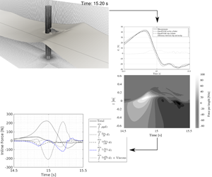


1 Introduction
Nonlinear loads from steep waves are important for a safe design of offshore substructures. Higher harmonic load components can induce a ringing response and have received strong attention during the last three decades. Another phenomenon, related to force histories of highly nonlinear waves, is the secondary load cycle, which manifests itself by an additional peak in the inline force history close to the following force minimum. The secondary load cycle has sometimes been linked to ringing, see for example Chaplin, Rainey & Yemm (Reference Chaplin, Rainey and Yemm1997), although higher harmonic forces are inherently present independently of whether a distinct secondary load cycle is present.
Several explanations have been suggested as the reason for the appearance of the secondary load cycle. However, there is not an agreement about the physical process which drives the secondary load cycle. The goal of the present paper is to study the cause of the secondary load cycle and the physical process behind it.
Grue, Bjørshol & Strand (Reference Grue, Bjørshol and Strand1994) were the first to report the existence of what was initially called a secondary oscillation in the force recordings. They characterized the starting time, period and amplitude of the oscillation in detail. They also reported that these oscillations occur approximately a quarter of the wave period after the main peak in the loading and has a period of as long as  $15\,\%$ of the wave period, with 11 % of the peak-to-peak amplitude of the total force. Grue et al. (Reference Grue, Bjørshol and Strand1994) argued that the experiments and the force recordings indicate the importance of the particle velocity under the wave crest and presence of the surface waves (which they related to the effect due to the gravity) in the problem. Hence, they suggested the Froude number,
 $Fr=u/\sqrt{gD}$, as a defining non-dimensional parameter where
 $u$ is the particle velocity below the crest,
 $g$ is the gravitational acceleration and
 $D$ is the cylinder diameter. A criterion,
 $Fr>0.4$, was suggested for the appearance of the secondary load cycle. They attributed the local phenomenon to a suction region one cylinder diameter below the still water level. The authors suggested that resonance between the free surface and the cylinder body may occur, which creates this suction and ultimately the secondary oscillation. Besides, the authors suggested that since the secondary oscillation happens a quarter of the wave period after the main peak of the inline force (force in the mean wave propagation direction,
 $F_{x}$), the marine substructure might experience a build-up of resonant responses.
Chaplin et al. (Reference Chaplin, Rainey and Yemm1997) conducted a set of experiments for the response of a single vertical cylinder in the inertia regime in steep non-breaking waves including discussions on the secondary load cycle. They used spring supports to adjust the stiffness of the cylinder, to place its natural frequencies in the range from 3 to 11 times the dominant wave frequency. The experiments were performed with three different cylinder diameters. It was found that the secondary load cycle has a significant effect on the response of the structures with natural frequencies close to the frequency of the secondary load cycle. The magnitude and period of the cycle were comparable to the results from Grue et al. (Reference Grue, Bjørshol and Strand1994), with a magnitude between 8 %–12 % of the total force range for the smallest and largest diameter cylinder, respectively, and a period of 15 % of the main force cycle period. They suggested that the secondary load cycle only appears significant when  $Fr>0.6$. They further suggested that
 $Fr$ is neither the sole influential parameter on the magnitude of the secondary load cycle nor the most important one. Instead, they proposed that the wave steepness is more influential in the magnitude of the secondary load cycle and for the largest waves the secondary load cycle magnitude decreases with increasing steepness while it is proportional to the cylinder diameter. They suggested that there is a direct relationship between the cubed diameter and the magnitude of the secondary load cycle. Further, the importance of the secondary load cycle in the ringing of the response cylinder was discussed.
Later on, Grue (Reference Grue2002) extended the analysis by more measurements and while he reported the same approximations for the relative magnitude and period of the secondary load cycle as in the initial investigation (Grue et al. Reference Grue, Bjørshol and Strand1994), he mentioned that appearance of the secondary load cycle depends on both cylinder diameter and the wave amplitude relative to the wavelength. He reported that the secondary load cycle occurs when the wavelength is larger than approximately 10 times the cylinder diameter. Grue (Reference Grue2002) stated that the secondary load cycle does not happen in the laboratory when the scale is too small and explained this phenomenon by the presence of flow separation. Grue & Huseby (Reference Grue and Huseby2002) investigated in more detail the effects of scale factor. They concluded that in the small scale, the secondary load cycle happens when the wave slope,  $k\unicode[STIX]{x1D702}_{m}$, exceeds 0.3 and for wavelength ratio,
 $kR$, smaller than 0.33 where
 $k$ is the wavenumber,
 $\unicode[STIX]{x1D702}_{m}$ is the crest height and
 $R$ is the cylinder radius. In the moderate scale, the secondary load cycle is more visible for waves with smaller slopes. The difference between the experiments in small and moderate scale was explained by the effect of flow separation. According to this work the secondary load cycle gives an important contribution to build-up of resonant body responses for a natural frequency of the structure approximately four times the local wave frequency.
Rainey (Reference Rainey2007) associated the secondary load cycle with the violent motion of the water surface. A cavity bubble is formed behind the cylinder which then collapses to give the secondary load cycle. He reported no connection between the secondary load cycle and the third harmonic of the wave frequency.
Paulsen et al. (Reference Paulsen, Bredmose, Bingham and Jacobsen2014b) investigated the secondary load cycle by computation of the interaction of regular stream function theory waves and a vertical circular cylinder. They concluded that for the analysed cases, the secondary load cycle was associated with force components at frequencies above the fifth and sixth harmonic of the fundamental wave frequency. It was also found that the magnitude of the secondary load cycle increases for decreasing values of  $kR$ in agreement with the observations of Grue (Reference Grue2002). The magnitude and period of the secondary load cycle were shown to depend largely on
 $H/H_{max}$ and to a lesser extent to
 $kh$ for the analysed cases where
 $H$ is the wave height,
 $H_{max}$ is the limiting wave height for a regular wave and
 $h$ is the water depth. They also stated by visual observation and a simplified analytical model that the secondary load cycle was caused by the free surface which drives a return flow from the back of the cylinder after the passage of the wave crest. A distinct vortex pair at the downstream side of the cylinder was shown to appear during the presence of a secondary load cycle. A simple potential flow model was used, to deduce that the force contribution from the secondary load cycle may be caused by the upstream propagating flow towards the front side of the cylinder and the associated downstream vortex pair.
In line with Rainey (Reference Rainey2007), Jose et al. (Reference Jose, Choi, Erik, Giljarhus and Gudmestad2017) explained the creation of the secondary load cycle by the blockage of the flow by the cylinder being filled by the diffracted waves, when they meet at the downstream side, and the resulting hump of water piled up at the back of the cylinder. This hump of water would create high pressure which would act in the opposite direction to that of the flow and exert a negative force on the back of the cylinder. Jose et al. (Reference Jose, Choi, Erik, Giljarhus and Gudmestad2017) also stated that correct turbulence modelling would contribute to an accurate estimation of the secondary load cycle. They did not, however, explain the reason for the importance of the turbulence in the characteristics of the secondary load cycle.
Kristiansen & Faltinsen (Reference Kristiansen and Faltinsen2017) suggested that the flow separation (governed by Keulegan–Carpenter number  $KC$) results in the local rear run-up. They conclude that the local rear run-up leads to the secondary load cycle, since it gives rise to the fourth and the fifth harmonics while reducing the third harmonic.
Riise et al. (Reference Riise, Grue, Jensen and Johannessen2018) investigated 2166 individual waves and separated the harmonics larger than 3.5 $\unicode[STIX]{x1D714}_{TT}$ from the force time series, where
 $\unicode[STIX]{x1D714}_{TT}$ is the trough-to-trough angular frequency of the wave. Regression methods were used to investigate the effect of
 $KC$, governing flow separation and
 $Fr$, free surface gravity wave effects, on the magnitude of the secondary load cycle. They concluded that both parameters are important while the best correlation was found between the secondary load cycle magnitude and an improved version of
 $Fr$. This may be explained through the initial definitions of
 $Fr$ and
 $KC$ in this study, which leads to
 $Fr=KC\sqrt{kD}/2\unicode[STIX]{x03C0}$ at deep water, such that
 $Fr$ offers an alternative, but not independent, ordering of the conventional properties
 $KC$ and
 $kD$ in the full parameter space. They showed a limiting threshold of
 $KC\approx 4{-}5$ or
 $Fr\approx 0.3{-}0.4$ which indicates a change in the physical mechanisms that govern the high-frequency force.
Other authors (Ghadirian, Bredmose & Dixen Reference Ghadirian, Bredmose and Dixen2016; Ghadirian, Bredmose & Schløer Reference Ghadirian, Bredmose and Schløer2017) have reported the presence of the secondary load cycles in laboratory measurements and computations without explaining the source of the phenomenon. From the literature review, it is observed that although the secondary load cycle is clearly a result of the wave–structure interaction and often linked to the flow at the back side of the cylinder, no precise account of the detailed flow mechanics causing it has been provided. The main goal of the present paper is to investigate the physical process in which the secondary load cycle is created. Experimental and numerical results of a focused wave group in one sea state are extensively used and analysed to separate the flow in different terms and identify the source of the secondary load cycle.
In § 2 the experimental set-up and the model are described. The models used and the numerical schemes with modified turbulence models implemented in OpenFOAM are defined. To increase the trust in the model, an extensive validation study for a set of basic cases is performed and presented in § 3. The cases include single-phase steady and oscillating flow around a cylinder which are close to the flow regimes of the investigated focused wave group. Afterwards, in § 4, the numerical results are validated in terms of free surface elevation, inline force and local pressure against measurements. Section 5 includes a detailed investigation of the flow by dividing the flow into horizontal disks and by calculating the pressure contribution from separate terms of the vertical Navier–Stokes equation. The role of the structural boundary layer and the force contribution from the vortices at the back of the cylinder is investigated in § 6 by comparison to a force computation with slip boundary conditions on the cylinder. Concluding remarks and suggested future work are presented in § 7.
2 Methodology
2.1 Experiments
The experiments were conducted at DHI Denmark in scale 1 : 50 as part of the DeRisk project (Bredmose et al. Reference Bredmose, Dixen, Ghadirian, Larsen, Schløer, Andersen, Wang, Bingham, Lindberg and Christensen2016). The shallow water wave basin used was 35 m long and 25 m wide. The investigated focused wave group was generated using a Joint North Sea Wave Project (JONSWAP) spectrum with laboratory-scale significant wave height of 0.15 m and peak period of 2.12 s at a water depth of 0.66 m. These conditions correspond to a 10 year return period climate in typical North Sea conditions close to the German Bight. The chosen wave height for the focused wave group (Tromans, Anatruk & Hagemeijer Reference Tromans, Anatruk and Hagemeijer1991) was 1.86 times the significant wave height,  $H_{s}$, of this sea state with no inclusion of directional spreading. Although the whole wave group was generated in the laboratory and numerically, only the results of the main wave in the focused wave group are shown in the present paper. The monopile was equipped with two force transducers, one at the top and one at the bottom of the cylinder with a laboratory scale diameter of 0.14 m. Based on the peak frequency wavenumber, these conditions are equivalent to
 $kh=0.85$ and
 $kR=0.09$.
Five pressure sensors were installed on the front side of the cylinder facing the wave-makers. The test was repeated eight times and the used measurements are ensemble-averaged over the eight repetitions. Linear wave generation theory (Dean & Dalrymple Reference Dean and Dalrymple1991) was used to calculate the piston type wave-maker position signals in the laboratory.
Reflection analysis was performed on the measured free surface elevation based on the work of Goda & Suzuki (Reference Goda and Suzuki1976) and Bredmose et al. (Reference Bredmose, Hunt-Raby, Jayaratne and Bullock2010) and less than 5 % reflection was observed from the artificial beach in the studied test.
Several methods were used to estimate  $KC$ and
 $Re$ values in the focused wave group defined as
 $$\begin{eqnarray}\displaystyle & \displaystyle KC=\frac{U_{m}}{f_{p}D}, & \displaystyle\end{eqnarray}$$
 $$\begin{eqnarray}\displaystyle & \displaystyle Re=\frac{U_{m}D}{\unicode[STIX]{x1D708}}. & \displaystyle\end{eqnarray}$$
Here  $U_{m}$ is either the maximum or the standard deviation of the horizontal velocity of the flow,
 $D$ is the diameter of the cylinder,
 $f_{p}$ is the peak frequency of the wave spectrum and
 $\unicode[STIX]{x1D708}$ is the kinematic viscosity of the fluid. The calculated non-dimensional numbers depend on choosing maximum or standard deviation of the velocity and the depth at which the velocity is sampled. In the experiments, the velocity was not measured. However, using the fully nonlinear potential flow solver OceanWave3D (Engsig-Karup, Bingham & Lindberg Reference Engsig-Karup, Bingham and Lindberg2009), the velocity time series at any height was calculated. Following Sumer & Fredsøe (Reference Sumer and Fredsøe2006),
 $KC$ and
 $Re$ were calculated using the standard deviation of the velocity at the still water level and were equal to 6 and
 $1\times 10^{4}$, respectively. Choosing the maximum velocity value at the maximum crest height (Yang & Rockwell Reference Yang and Rockwell2002) leads to a
 $KC$ value of 18 and a
 $Re$ value of
 $1.7\times 10^{5}$ and at the half-depth (Yang & Rockwell Reference Yang and Rockwell2002) leads to
 $KC$ and
 $Re$ values of
 $6.4$ and
 $5.8\times 10^{4}$, respectively. The calculation of the
 $KC$ and
 $Re$ is important for recognition of the flow regime around the cylinder.
2.2 The numerical model
The coupled solver OceanWave3D–Waves2Foam (Paulsen Reference Paulsen2013; Paulsen, Bredmose & Bingham Reference Paulsen, Bredmose and Bingham2014a) was used to reproduce the experiment. Waves2Foam is an extension to the InterFoam solver of OpenFOAM (Weller et al. Reference Weller, Tabor, Jasak and Fureby1998) which uses relaxation zones to induce incident gravity waves (Jacobsen, Fuhrman & Fredsøe Reference Jacobsen, Fuhrman and Fredsøe2012) in the domain. InterFoam uses a volume of fluid (known as VOF) method to treat the free surface flow (Hirt & Nichols Reference Hirt and Nichols1981). It solves the continuity equation and the momentum conservation equations
 $$\begin{eqnarray}\displaystyle & \displaystyle \frac{\unicode[STIX]{x2202}u_{i}}{\unicode[STIX]{x2202}x_{i}}=0, & \displaystyle\end{eqnarray}$$
 $$\begin{eqnarray}\displaystyle & \displaystyle \frac{\unicode[STIX]{x2202}\unicode[STIX]{x1D70C}u_{i}}{\unicode[STIX]{x2202}t}+u_{j}\frac{\unicode[STIX]{x2202}\unicode[STIX]{x1D70C}u_{i}}{\unicode[STIX]{x2202}x_{j}}=-\frac{\unicode[STIX]{x2202}p^{\ast }}{\unicode[STIX]{x2202}x_{i}}-g_{j}x_{j}\frac{\unicode[STIX]{x2202}\unicode[STIX]{x1D70C}}{\unicode[STIX]{x2202}x_{i}}+\frac{\unicode[STIX]{x2202}}{\unicode[STIX]{x2202}x_{j}}(2\unicode[STIX]{x1D707}_{eff}\unicode[STIX]{x1D61A}_{ij})+\unicode[STIX]{x1D70E}_{T}\unicode[STIX]{x1D705}\frac{\unicode[STIX]{x2202}\unicode[STIX]{x1D6FC}}{\unicode[STIX]{x2202}x_{i}}, & \displaystyle\end{eqnarray}$$
 $$\begin{eqnarray}\displaystyle & \displaystyle \unicode[STIX]{x1D61A}_{ij}=\frac{1}{2}\left(\frac{\unicode[STIX]{x2202}u_{i}}{\unicode[STIX]{x2202}x_{j}}+\frac{\unicode[STIX]{x2202}u_{j}}{\unicode[STIX]{x2202}x_{i}}\right), & \displaystyle\end{eqnarray}$$
where  $u_{i}$ are the velocity components,
 $x_{i}$ are the coordinates,
 $\unicode[STIX]{x1D70C}$ is the local fluid density,
 $p^{\ast }$ is the pressure minus the hydrostatic potential
 $\unicode[STIX]{x1D70C}g_{j}x_{j}$,
 $g_{j}$ is the gravitational acceleration,
 $\unicode[STIX]{x1D707}_{eff}$ is the local effective viscosity and
 $\unicode[STIX]{x1D61A}_{ij}$ is the mean strain rate tensor. The effective viscosity,
 $\unicode[STIX]{x1D707}_{eff}$, is calculated as
 $\unicode[STIX]{x1D707}_{eff}=\unicode[STIX]{x1D707}+\unicode[STIX]{x1D707}_{t}$, where
 $\unicode[STIX]{x1D707}$ is the local dynamic viscosity and
 $\unicode[STIX]{x1D707}_{t}$ is the turbulent viscosity (Menter, Kuntz & Langtry Reference Menter, Kuntz and Langtry2003). The turbulent viscosity was set to zero for the computations with a slip boundary condition on the cylinder wall. The viscosity of the fluid, however, was considered in all of the computations. The fluid fraction is denoted by
 $\unicode[STIX]{x1D6FC}$ which can take values between 0 and 1 for full air and water occupation of the cells, respectively. Local fluid properties are calculated by linear weighting between the water and air properties, e.g.
 $\unicode[STIX]{x1D6F7}=\unicode[STIX]{x1D6FC}\unicode[STIX]{x1D6F7}_{water}+(1-\unicode[STIX]{x1D6FC})\unicode[STIX]{x1D6F7}_{air}$, where
 $\unicode[STIX]{x1D6F7}$ represents any needed fluid property. Hence,
 $\unicode[STIX]{x1D707}_{eff}=\unicode[STIX]{x1D6FC}\unicode[STIX]{x1D707}_{water}+(1-\unicode[STIX]{x1D6FC})\unicode[STIX]{x1D707}_{air}+\unicode[STIX]{x1D707}_{t}$ in each cell. The last term in (2.4) takes the surface tension,
 $\unicode[STIX]{x1D70E}_{T}$, into account by considering the surface curvature,
 $\unicode[STIX]{x1D705}$, in the border of the two phases where the gradient of
 $\unicode[STIX]{x1D6FC}$ is non-zero. In our calculations, this term is ignored.
The transport equation of  $\unicode[STIX]{x1D6FC}$ is
 $$\begin{eqnarray}\frac{\unicode[STIX]{x2202}\unicode[STIX]{x1D6FC}}{\unicode[STIX]{x2202}t}+\frac{\unicode[STIX]{x2202}\unicode[STIX]{x1D6FC}u_{j}}{\unicode[STIX]{x2202}x_{j}}+\frac{\unicode[STIX]{x2202}}{\unicode[STIX]{x2202}x_{j}}(\unicode[STIX]{x1D6FC}(1-\unicode[STIX]{x1D6FC})u_{j}^{r})=0,\end{eqnarray}$$
where  $u_{j}^{r}$ has the unit of velocity and is in the normal direction to the air–water interface. The last term compresses the region where
 $\unicode[STIX]{x1D6FC}$ is between 0 and 1. More information on the performance of this term can be found in Deshpande, Anumolu & Trujillo (Reference Deshpande, Anumolu and Trujillo2012).
To reproduce the measurements, the wave paddle signal was created from the first-order wave generation similarly to the experiments (Dean & Dalrymple Reference Dean and Dalrymple1991) and the velocity of the paddles was used as a flux boundary condition in the nonlinear potential flow solver OceanWave3D (Engsig-Karup et al. Reference Engsig-Karup, Bingham and Lindberg2009). This method of generation is linearly consistent with the piston wave generation in the laboratory. Differences at higher orders are expected because no piston or boundary movement is included in the model. However, good consistency with experiments using this approach has been presented in earlier work (Paulsen et al. Reference Paulsen, Bredmose and Bingham2014a) and as part of DeRisk project (Bredmose et al. Reference Bredmose, Dixen, Ghadirian, Larsen, Schløer, Andersen, Wang, Bingham, Lindberg and Christensen2016; Ghadirian et al. Reference Ghadirian, Bredmose and Dixen2016, Reference Ghadirian, Bredmose and Schløer2017). A top view of the computational domains is shown in figure 1. The embedded OpenFOAM domain was driven with waves generated in OceanWave3D through a relaxation zone (Jacobsen et al. Reference Jacobsen, Fuhrman and Fredsøe2012).
Schematic drawing of the numerical domains including the potential flow fully nonlinear solver OceanWave3D domain and the Navier–Stokes solver OpenFOAM domain.

Convergence tests were performed to verify that all the significant waves in the sea state, even with the highest frequency, were resolved. From these studies, it was observed that in the OceanWave3D domain a discretization by  $501\times 1\times 15$ cells with constant time step
 $\unicode[STIX]{x1D6FF}t=0.01~\text{s}$ was numerically converged more than 99 % meaning that the results would change less than 1 % by refining the mesh. The OceanWave3D results were mapped inside the OpenFOAM domain in each time step in a 3 m long relaxations zone. The OpenFOAM mesh with
 $\text{d}x=0.02~\text{m}$ and with a cell aspect ratios close to one showed less than 1 % change in the free surface elevation and inline force results when the mesh resolution was doubled in all directions. Nevertheless, for better resolution of the vortices around the cylinder, the finest mesh was used with
 $\text{d}x=0.01~\text{m}$ and
 $24\times 10^{6}$ cells.
For turbulence modelling, the  $k\unicode[STIX]{x1D714}$–SST model implemented in OpenFOAM was used. The implementation is based on Menter et al. (Reference Menter, Kuntz and Langtry2003) without the density in the transport equations in OpenFOAM which was added following the work of Brown et al. (Reference Brown, Magar, Greaves and Conley2014) and Devolder, Rauwoens & Troch (Reference Devolder, Rauwoens and Troch2017). The resulting equations are
 $$\begin{eqnarray}\displaystyle & \displaystyle \frac{\unicode[STIX]{x2202}\unicode[STIX]{x1D70C}k}{\unicode[STIX]{x2202}t}+\frac{\unicode[STIX]{x2202}\unicode[STIX]{x1D70C}u_{j}k}{\unicode[STIX]{x2202}x_{j}}-\frac{\unicode[STIX]{x2202}}{\unicode[STIX]{x2202}x_{j}}\left(\unicode[STIX]{x1D6E4}_{k}\frac{\unicode[STIX]{x2202}k}{\unicode[STIX]{x2202}x_{j}}\right)=\unicode[STIX]{x1D70C}P_{k}-\unicode[STIX]{x1D6FD}^{\ast }\unicode[STIX]{x1D70C}\unicode[STIX]{x1D714}k, & \displaystyle\end{eqnarray}$$
 $$\begin{eqnarray}\displaystyle & \displaystyle \frac{\unicode[STIX]{x2202}\unicode[STIX]{x1D70C}\unicode[STIX]{x1D714}}{\unicode[STIX]{x2202}t}+\frac{\unicode[STIX]{x2202}\unicode[STIX]{x1D70C}u_{j}\unicode[STIX]{x1D714}}{\unicode[STIX]{x2202}x_{j}}-\frac{\unicode[STIX]{x2202}}{\unicode[STIX]{x2202}x_{j}}\left(\unicode[STIX]{x1D6E4}_{\unicode[STIX]{x1D714}}\frac{\unicode[STIX]{x2202}\unicode[STIX]{x1D714}}{\unicode[STIX]{x2202}x_{j}}\right)=\unicode[STIX]{x1D70C}\frac{\unicode[STIX]{x1D6FE}}{\unicode[STIX]{x1D708}_{t}}G-\unicode[STIX]{x1D6FD}\unicode[STIX]{x1D70C}\unicode[STIX]{x1D714}^{2}+\unicode[STIX]{x1D70C}2(1-F_{1})\frac{\unicode[STIX]{x1D70E}_{\unicode[STIX]{x1D714}2}}{\unicode[STIX]{x1D714}}\frac{\unicode[STIX]{x2202}k}{\unicode[STIX]{x2202}x_{j}}\frac{\unicode[STIX]{x2202}\unicode[STIX]{x1D714}}{\unicode[STIX]{x2202}x_{j}},\quad & \displaystyle\end{eqnarray}$$
where
 $$\begin{eqnarray}\unicode[STIX]{x1D6E4}_{k}=\unicode[STIX]{x1D707}+\unicode[STIX]{x1D707}_{t}\unicode[STIX]{x1D70E}_{k},\quad \unicode[STIX]{x1D6E4}_{\unicode[STIX]{x1D714}}=\unicode[STIX]{x1D707}+\unicode[STIX]{x1D707}_{t}\unicode[STIX]{x1D70E}_{\unicode[STIX]{x1D714}},\end{eqnarray}$$
 $$\begin{eqnarray}G=\unicode[STIX]{x1D708}_{t}\unicode[STIX]{x1D70F}_{ij}\frac{\unicode[STIX]{x2202}u_{i}}{\unicode[STIX]{x2202}x_{j}},\quad P_{k}=\min (G;c_{1}\unicode[STIX]{x1D6FD}^{\ast }k\unicode[STIX]{x1D714}),\end{eqnarray}$$
 $$\begin{eqnarray}\unicode[STIX]{x1D707}_{t}=\unicode[STIX]{x1D70C}\frac{a_{1}k}{\max (a_{1}\unicode[STIX]{x1D714};S\cdot F_{2})}.\end{eqnarray}$$
The constants,  $\unicode[STIX]{x1D70E}_{k}$,
 $\unicode[STIX]{x1D70E}_{\unicode[STIX]{x1D714}}$,
 $\unicode[STIX]{x1D6FD}$ and
 $\unicode[STIX]{x1D6FE}$ are chosen and computed according to Brown et al. (Reference Brown, Magar, Greaves and Conley2014) among others. The resulting
 $k$ and
 $\unicode[STIX]{x1D714}$ from solving (2.7) and (2.8) are used to calculate
 $\unicode[STIX]{x1D707}_{t}$, required in (2.4).
The convergence tests were performed to find the optimum combination of Courant number and the discretization schemes based on the work by Eltard, Fuhrman & Roenby (Reference Eltard, Fuhrman and Roenby2017). A summary of the model set-up is presented in table 2 in Appendix. The upwind scheme was used for the divergence term of the turbulence quantities  $k$ and
 $\unicode[STIX]{x1D714}$.
The coupling of the pressure and velocity equations was done by the PIMPLE solver, which is a combination of two algorithms: the semi-implicit method for pressure-linked equations (known as SIMPLE) and the pressure-implicit split operator (PISO). While ‘smoothsolver’ was used for  $\unicode[STIX]{x1D6FC}$,
 $k$ and
 $\unicode[STIX]{x1D714}$ linear equations, the pressure equation was solved by the generalized geometric–algebraic multi-grid (known as GAMG) and the velocity by the preconditioned bi-conjugate gradient (known as PBiCG) with diagonal incomplete-LU (known as DILU) pre-conditioner (Greenshields Reference Greenshields2015). It was observed that the most consistent results to the measured free surface elevation were obtained when the number of outer corrections in the PIMPLE solver was set to one, which practically makes this solver the PISO solver. It was checked that the residuals were below
 $10^{-3}$ in all the computations to make sure the results are converged in each time step.
The boundary conditions of the domain are shown in table 3 in Appendix. The boundary conditions on the sea bed and the sidewalls were of type zeroGradient for all quantities. The boundary condition of the velocity on the cylinder wall was defined as fixed zero in this table. However, computations with slip boundary condition on the cylinder were also performed to compare its effect. The length of the domain was defined by the wavelength and the fact that the relaxation zones in the OpenFOAM domain should be at least as long as the longest wave mapped in the domain (Jacobsen et al. Reference Jacobsen, Fuhrman and Fredsøe2012; Jacobsen Reference Jacobsen2017). However, since the focused wave group contains very long waves in the spectrum of the sea state a reflection analysis was performed to find the shortest relaxation zone length for which reflected waves are smaller than 5 %. In addition, it was observed that the quality of propagation of the waves depends drastically on the aspect ratio of the cells around the free surface. The aspect ratio should be as close to 1 as possible and even an aspect ratio of 2 diminishes the performance of the solver (Jacobsen Reference Jacobsen2011; Paulsen Reference Paulsen2013; Eltard et al. Reference Eltard, Fuhrman and Roenby2017). This limitation in the aspect ratio limited the ability of resolving the boundary layer at the cylinder wall. It was also observed that refining the mesh in the radial direction around the cylinder introduced artificial waves around the cylinder which affects the inline force time series on the cylinder. Hence using a uniform mesh in the domain with a wall function on the cylinder wall was found to be the most viable solution.
3 Model validation against basic flows
The numerical set-up with the same discretization as described in the previous section was validated against cases of channel flow and steady and oscillating single-phase flow around a cylinder.
The simplest validation case was to investigate if the model is capable of capturing the law of the wall of a steady channel flow over a smooth wall. In figure 2(a) the validity of the model is shown in comparison to theory from von Kármán (Reference von Kármán1931).
The theoretical equations used in figure 2(a) are given by
 $$\begin{eqnarray}\frac{\overline{u}}{U_{f}}=\left\{\begin{array}{@{}ll@{}}y^{+}, & y^{+}<5,\\ 2.5\ln y^{+}+5, & 30<y^{+}<500.\end{array}\right.\end{eqnarray}$$
Here  $y^{+}=yU_{f}/\unicode[STIX]{x1D708}$ is the non-dimensional wall distance,
 $U_{f}$ is the friction velocity,
 $\unicode[STIX]{x1D708}$ is the kinematic viscosity,
 $\overline{u}$ is the average velocity and
 $y$ is the normal distance from the wall. The viscous sublayer, buffer layer and log-law region are resolved and predicted very well in the inner layer of the flow.
The validity of the model in comparison with the measurements conducted by Jensen, Sumer & Fredsøe (Reference Jensen, Sumer and Fredsøe1989) in the calculation of the friction coefficient in the wave boundary layer over a smooth wall is shown in figure 2(b). Two sets of computations were performed to validate the model with and without using the wall function. The first set of the computations, carried out for a range of  $Re$ values from
 $8.5\times 10^{3}$ to
 $1.6\times 10^{6}$, resolved the boundary layer with
 $y^{+}$ values smaller than 1 in the first cell for all cases. The results of this group are consistent with the measurements except in the transition region,
 $1.5\times 10^{5}<Re<7\times 10^{5}$. It should be noted that the behaviour of the flow in this region is in general associated with some scatter for the friction coefficient since different experiments also obtain different friction coefficients (Jensen et al. Reference Jensen, Sumer and Fredsøe1989; Fredsøe et al. Reference Fredsøe, Sumer, Kozakiewicz, Chua and Deigaard2003). The second group of simulations was for a larger range of
 $Re$ values with
 $y^{+}$ values larger than 30 next to the wall. The results for this group for
 $Re$ values larger than
 $1\times 10^{5}$ are also consistent with the experiments.
(a) The law of the wall. The solid black line shows the model results while the dashed lines show the theory from (3.1). (b) Wave boundary layer.

To validate the model in flows around bluff bodies, cases of steady flow around a cylinder with different  $Re$ values were simulated and the drag coefficient (
 $C_{d}$) and Strouhal number (
 $St$) were compared with experimental results represented in Sumer & Fredsøe (Reference Sumer and Fredsøe2006) and computational results from Rosetti, Vaz & Fujarra (Reference Rosetti, Vaz and Fujarra2012), Stringer, Zang & Hillis (Reference Stringer, Zang and Hillis2014) and Ye & Wan (Reference Ye and Wan2017). Here
 $St=fD/u$ where
 $f$ is the vortex shedding frequency,
 $D$ is the cylinder diameter and
 $u$ is the flow velocity. It is shown in figure 3 that the results obtained using the current model and set-up can give among the most consistent results with the measurements up to
 $Re$ of
 $1\times 10^{5}$. However, the results for
 $Re=1\times 10^{6}$, in the super critical region, are not as consistent with the measurements. The inconsistency in this range is expected since the Reynolds-averaged Navier–Stokes simulations do not usually capture the correct behaviour of the flow above the subcritical regime (Rosetti et al. Reference Rosetti, Vaz and Fujarra2012; Stringer et al. Reference Stringer, Zang and Hillis2014; Ye & Wan Reference Ye and Wan2017). For the cases of the present paper,
 $Re$ is below
 $1.7\times 10^{5}$. The solver is therefore considered sufficiently accurate for the flow regimes studied.
(a) Drag coefficient as a function of  $Re$ for a steady flow around the cylinder. (b) Here
 $St$ as a function of
 $Re$ for a steady flow around cylinder. Results from three studies (Rosetti et al. Reference Rosetti, Vaz and Fujarra2012; Stringer et al. Reference Stringer, Zang and Hillis2014; Ye & Wan Reference Ye and Wan2017) are included for comparison. The background plot shows the experiments represented in Sumer & Fredsøe (Reference Sumer and Fredsøe2006).

The next validation case is 2-D oscillatory flow around a circular cylinder. In figure 4 the drag and inertia coefficients for three Reynolds and  $KC$ values corresponding to the free surface flow at the crest, still water level and in half-depth of 0.33 m are shown. In these computations the wall function was used on the cylinder wall and the boundary layer was not resolved. From figure 4(a) it is observed that the inertia coefficient is over-predicted less than 3 % in all cases with
 $KC$ values of 6, 12 and 18. For the drag coefficient there is an under-prediction of less than 14 % as shown in figure 4(b). In general a good agreement between the simulation results and the measurements is shown.
Drag and inertia coefficients of oscillating flow around the cylinder with three Reynolds and  $KC$ covering the flow regimes of the free surface flow at three heights. (a) Inertia coefficient. (b) Drag coefficient. The background plot shows the experiments represented in Sumer & Fredsøe (Reference Sumer and Fredsøe2006).

(a) Inline force time series. (b) Free surface elevation. (c) Run-up from the OpenFOAM simulations.

Wave-induced pressure at five different heights on the front side of the cylinder.

4 Validation of the model results with experiments
We now turn to the recomputation of the ensemble-averaged focused wave group. In figure 5(a) the ensemble-averaged measured time series of inline force is presented. The standard deviation between the eight repetitions of the inline force and free surface elevations is shown with the grey area around the mean value curves. However, because of high repeatability, the deviation areas are hardly visible in this panel. It is observed that the maximum inline force happens at 14.8 s, hereafter referred to as the first peak. The horizontal axes are limited to the event of interest, the secondary load cycle. Six time instances from 15 s to 15.5 s, every 0.1 s, are also shown in this panel with dotted lines for clarity. Two local minima are observed in the force time series at 15.1 s and 15.32 s with a maximum in-between which hereafter are referred to as the first dip, the second dip and the second peak. The simulation results of inline force are presented in the same panel (figure 5a). The OpenFOAM results are in good agreement with the measurements. OpenFOAM also shows a good reproduction of the secondary load cycle phenomenon.
The free surface elevation at the monopile centre (measured five diameters away from the cylinder) is shown in figure 5(b). The measured time series is maximum at 14.92 s which indicates a phase shift between the inline force and the free surface elevation which is in agreement with the known characteristics of an inertia-dominant flow. The free surface elevation is also presented in figure 5(b) and shows a good agreement with the measurements. However, the measured wave is slightly more symmetric than the computations. Since the wave paddles in the computations were only linearly consistent with the experiments these minor differences are expected.
In figure 5(c) the run-up on the front and back side of the cylinder and the difference between them is shown from the OpenFOAM results. In addition, a free shoot and fall trajectory from the maximum run-up on both sides is presented. The water on the front side is thrown up at 14.85 s with only gravity imposing a force on it. Hence its trajectory is similar to the free shoot trajectory. After 15 s the run-up water falls faster than free fall. On the back side the run-up water is moved up and down slower than free shoot and fall peaking at 15.1 s. The difference in the run-up on the front and the back side is a simple representation of the possible hydrostatic force contributions to the force history from the front and back flows. From the curve though, a different time scale than the secondary load cycle is visible. The secondary load cycle can thus not be explained by hydrostatic effects related to the run-up and down flows at the front and back side.
The wave-induced pressure time series measured at five heights of 0.16 m, 0.12 m, 0.08 m,  $-0.14~\text{m}$ and
 $-0.18~\text{m}$ from the still water level in the experiments are shown in figure 6. The measurement heights are presented above each panel. The wave-induced pressure is calculated as
 $$\begin{eqnarray}p_{wave}=\left\{\begin{array}{@{}ll@{}}p_{total}+\unicode[STIX]{x1D70C}gz, & z<0,\\ p_{total}, & z\geqslant 0,\end{array}\right.\end{eqnarray}$$
which represents the pressure added to the gauge pressure in calm water conditions.
From figure 6 we can see that the pressure sensors that are always wet show positive and negative wave-induced pressure similar to a sine wave, but the pressure sensors that are above the still water level and are sometimes dry show non-zero values only when wet during the run-up time on the front side. It is worth mentioning that the maximum wave-induced pressure measured at 12 cm above the still water level is smaller than the ones measured at higher and lower heights. Small oscillations in the pressures above still water level are seen just after they become dry. This is likely to be a spurious feature of the pressure sensor or due to aeration effects.
In the same figure, wave-induced pressures from computations with slip and no-slip boundary condition on the cylinder are shown. The differences between the two calculations are very small and the agreement between the results and the measurements is generally good. The main differences are a small offset for the lower transducers, some amplitude difference for the upper transducers and lower maximum pressure at 12 cm than at 16 cm. These are very likely related to slight differences in the waves that are reproduced in the computations. The absence of surface tension in the numerical set-up may also have an effect on the run-up height and the resulting pressures.
Even with these observed differences, we note that the temporal variation of the pressures is very well reproduced. Given further the good match of the inline force and free surface elevation, we regard the numerical results to be a sufficiently accurate reproduction of the physical wave–structure interaction to warrant further detailed analysis of the secondary load cycle and the associated flow.
Snapshots of the free surface: (a) at the time of the wave crest passing the back side of the cylinder, (b) when the water column is fully formed behind the cylinder (maximum run-up behind the cylinder), (c) at the beginning of the secondary load cycle (collapse of the water column), (d) at the time of the local minimum of the secondary load cycle, (e) at the end of the secondary load cycle, (f) after the end of the secondary load cycle.

5 Detailed investigations
In figure 7 the free surface of the flow is shown for the six time instants marked with dotted lines in figure 5(a). In figure 7(a), at 15.0 s, the run-up on the front side is maximum. The wave crest is just on the back side of the cylinder. A distinct water column (mound) has already been formed at the back side. In figure 7(b), at 15.1 s, the run-up on the back side starts to fall down. This is the same time when the first dip occurs in the inline force time series. The water column is extending in length from the back of the cylinder until the wave crest which is 1.5 diameters behind the cylinder.
At 15.2 s, figure 7(c), when also the second peak occurs, the water column still distinctly exists. Even though the run-up on the back side has decreased, the free surface elevation of the outer wave flow has decreased so much that the relative height of the water column is larger than before. The water column width at the base of the water column has spread. In figure 7(d), at 15.3 s, when the second dip occurs, there is a backward water flow towards the front of the cylinder. The height of the water column has drastically decreased. At 15.4 s, figure 7(e), two water jets created from the initial collapse of the water column have reached the front side. Two further side waves from the collapse of the water column have started to spread towards the outer flow. In figure 7(f), time 15.5 s, the remaining part of the water column is disappearing. Also, the created second pair of waves from the collapse of the water column have started to disappear. Some surface disturbance can still be seen around the cylinder.
We now turn to a more detailed investigation of the flow and forces associated with the secondary load cycle. The vertical distribution of the inline force time series is first visualized and then detailed into contributions from the front and back sides to isolate the secondary load cycle. Afterwards, we divide the pressure on the cylinder into different terms of the vertical momentum equation. Because we have all the variables in the numerical domain and around the cylinder, we can recompute the different terms. It should be mentioned that all the results presented in this section are analyses of the computations and not the measurements. However, since the validity of the model is demonstrated in the previous section, we regard the results extendable to the details of the physical flow.
To explain the flow in more detail a few terms for describing the physical events related to vertical run-up and run-down flows are given. A throw-up event is defined as shooting the water upwards in the form of a water jet. The most intuitive example of a throw-up event is when the steep wave hits the cylinder (or a flat vertical wall) and shoots a water jet upwards. The pressure effect of the throw-up event is associated with positive acceleration of the water particles in the vertical direction (i.e.  $\unicode[STIX]{x2202}\unicode[STIX]{x1D70C}u_{z}/\unicode[STIX]{x2202}t\gg 0$). A suction event on the back side of the cylinder is related to the decreasing acceleration of the water column when the water below has been moved away because of the incident wave kinematics. This suction event is associated with
 $\unicode[STIX]{x2202}\unicode[STIX]{x1D70C}u_{z}/\unicode[STIX]{x2202}t\ll 0$. A wash-down event occurs when there is a high-velocity flow on the cylinder wall and it is associated with the
 $u_{z}\unicode[STIX]{x2202}\unicode[STIX]{x1D70C}u_{z}/\unicode[STIX]{x2202}z$ term. Finally, a catch pressure effect is observed when lower layers of the fluid decelerate the falling fluid above them and it occurs when
 $\unicode[STIX]{x2202}\unicode[STIX]{x1D70C}u_{z}/\unicode[STIX]{x2202}t>0$ and
 $u_{z}<0$. Wash-down and catching usually occur simultaneously with wash-down possibly leading the process.
5.1 Vertical distribution of inline force
The inline force is plotted in a contour plot with the axis of time and height on the cylinder measured from the still water level ( $z$-axis of the coordinate system) in figure 8. The plot is obtained by integration of the computational pressure on the cylinder wall in the azimuth direction. At 15.1 s, a minimum force appears to be caused by a local low-force event close to the still water level followed by a higher force event at 15.2 s that propagates from above. Finally, the second force minimum at 15.32 s is related to another local low-force event which extends down to 1.5 times the diameter. Hence, in this figure, it is observed that the secondary load cycle is visible in the heights closer to the still water level from 15.1 s to 15.4 s and its effect extends to 1.5 diameters below the still water level (figure 8).
Contour plot of inline force per length as a function of height and time. Integrating in height leads to the total inline force time series. The white dashed lines indicate the time instants 15.1 s, 15.2 s and 15.32 s, the first local minimum, the local maximum and the second local minimum of the secondary load cycle, respectively.

5.2 Azimuthal and vertical distribution of inline force
The front side and the back side inline force per unit length of the cylinder are separately shown in figure 9 for the various vertical positions where the secondary load cycle effect was distinctly visible. The total force per unit height is shown in the blue curve while the front side force per unit height is shown in black dashed-dot lines and the back side force per unit height is shown in the black dashed line. The force per length from the back side is multiplied by minus one so that visual comparison with the front side is easier. In these panels, an event resembling the secondary load cycle can be observed in the same time period as in the total inline force time series. From  $z=0.04~\text{m}$ to
 $z=-0.05~\text{m}$ the secondary load cycle correlates to a cycle of decrease and increase from 15.2 s to 15.4 s in the absolute value of the inline force on the back side. Similar behaviour is observed from
 $z=-0.09~\text{m}$ to
 $z=-0.21~\text{m}$ with a smaller cycle until at
 $z=-0.28~\text{m}$ where it has almost completely disappeared. The front side force time series shows an abrupt decrease at around 15.15 s to 15.30 s from
 $z=0.04~\text{m}$ to
 $z=-0.09~\text{m}$ at the same time as the second peak in the total force per length at the same height. Hence, the first dip and the subsequent peak in the total inline force time series cannot be related to a distinct event at either front or back. The second dip occurs when the water from the front side is washed down and a sudden stop of force decrease occurs on the back side.
Separated front side, back side and total forces per unit height.

5.3 Detailed study by the vertical momentum equation
To understand the nature of the secondary load cycle more closely, the vertical momentum conservation equation is used to separate the local pressure contribution from each term. Equation (2.4) can be rewritten in cylindrical coordinates with total pressure,  $p$, instead of
 $p^{\ast }$ to be used easily around the cylinder
 $$\begin{eqnarray}\frac{\unicode[STIX]{x2202}\unicode[STIX]{x1D70C}u_{z}}{\unicode[STIX]{x2202}t}+u_{r}\frac{\unicode[STIX]{x2202}\unicode[STIX]{x1D70C}u_{z}}{\unicode[STIX]{x2202}r}+\frac{u_{\unicode[STIX]{x1D703}}}{r}\frac{\unicode[STIX]{x2202}\unicode[STIX]{x1D70C}u_{z}}{\unicode[STIX]{x2202}\unicode[STIX]{x1D703}}+u_{z}\frac{\unicode[STIX]{x2202}\unicode[STIX]{x1D70C}u_{z}}{\unicode[STIX]{x2202}z}=-\frac{\unicode[STIX]{x2202}p}{\unicode[STIX]{x2202}z}+g_{z}z+\text{viscous terms}.\end{eqnarray}$$
The surface tension term in (2.4) has been dismissed since it was not included in our computations. The vertical momentum equation has the benefit that it separates the hydrostatic terms from the other terms. The values from the OpenFOAM domain in Cartesian coordinates were transferred into the cylindrical coordinates for these analyses. In figure 10 the cylindrical coordinate system and the cells around the cylinder are shown as from above.
The cylindrical coordinates and the cells around the cylinder, shown as from above. The cylinder is facing the waves at  $\unicode[STIX]{x1D703}=\unicode[STIX]{x03C0}$.

The polar momentum equation can be rewritten to separate the sources of pressure
 $$\begin{eqnarray}\displaystyle p(z) & = & \displaystyle \int _{z}^{atm}(\unicode[STIX]{x1D70C}g)\,\text{d}z\nonumber\\ \displaystyle & & \displaystyle +\,\int _{z}^{atm}\left(\underbrace{\displaystyle \frac{\unicode[STIX]{x2202}\unicode[STIX]{x1D70C}u_{z}}{\unicode[STIX]{x2202}t}+\frac{u_{\unicode[STIX]{x1D703}}}{r}\frac{\unicode[STIX]{x2202}\unicode[STIX]{x1D70C}u_{z}}{\unicode[STIX]{x2202}\unicode[STIX]{x1D703}}+u_{z}\frac{\unicode[STIX]{x2202}\unicode[STIX]{x1D70C}u_{z}}{\unicode[STIX]{x2202}z}+u_{r}\frac{\unicode[STIX]{x2202}\unicode[STIX]{x1D70C}u_{z}}{\unicode[STIX]{x2202}r}}_{\displaystyle \frac{\text{D}\unicode[STIX]{x1D70C}u_{z}}{\text{D}t}}+\text{viscous terms}\right)\text{d}z.\qquad\end{eqnarray}$$
To calculate the pressure contribution from the terms on the right-hand side of (5.2) we started from the top of the domain  $atm$ (atmosphere) where the pressure was close to zero. Hence the effect of the forces from the air on the cylinder were negligible which is expected considering the ratio of the density between water and air. The total pressure on the left-hand side is known from the computational results. The pressure contribution from
 $u_{r}(\unicode[STIX]{x2202}\unicode[STIX]{x1D70C}u_{z}/\unicode[STIX]{x2202}r)$ plus the viscous terms were thus calculated from the difference between the total pressure and the other calculated terms on the right-hand side. This process was repeated for 170 azimuth angles to get the pressure distribution around the cylinder from each term. The calculated total force from the cell centre pressure values was calculated and was found identical to the face value results. Therefore, it was justified to use the pressure and velocity component values from the cell centres closest to the cylinder wall for the analysis.
The inline force resulting from each term of (5.2) is shown in figure 11. It can be seen that the time series from the term  $\unicode[STIX]{x2202}\unicode[STIX]{x1D70C}u_{z}/\unicode[STIX]{x2202}t$ peaks at 15.2 s similar to the secondary load cycle. The hydrostatic force time series has a minimum at around 15.26 s which is close to the second dip of the secondary load cycle. However, since from figure 9 it is clear that the forces should be investigated more locally, a side and height divided analysis of these results is next carried out.
The forces originated from different terms of the Navier–Stokes equation in the vertical direction in cylindrical coordinate system.

In figures 12 and 13, the force per unit height contour plots for the major subterms of (5.2) are visualized. Each row is assigned to either the total pressure or one subterm. From left to right, each column is attributed to the contribution from both sides, front side and back side, respectively. In all the contour plots, the time instants 15.10 s, 15.20 s and 15.32 s are marked for reference to the secondary load cycle with vertical dashed lines. The contours of force per metre height from the total pressure are shown in the first row of figure 12. Figure 12(a) is the same contour plot as presented in figure 8. Figure 12(b) visualizes the force per length on the front side of the cylinder and shows some small local phenomena by increased proximity of contour lines at the same period as the secondary load cycle. At around 15.15 s the front side force begins to decrease faster. The differences in the rate of change in this contour plot can be judged from the proximity of the contour lines. Figure 12(c) shows the forces only on the back side of the cylinder where a local cycle can be seen in the contour lines from 15.15 s to 15.35 s. The local cycle can be seen in the contour lines down to 1.5 diameters from just above the still-water level.
The second row includes plots of forces from the hydrostatic pressure term  $\int _{z}^{atm}(\unicode[STIX]{x1D70C}g)\,\text{d}z$ in (5.2). In figure 12(d), the total hydrostatic force per unit height is shown. It is observed that due to the integrated effect of the run-up around the cylinder the hydrostatic force is positive until 15.1 s. Afterwards, since the integrated run-up on the front side is smaller than on the back side, the inline force per unit length becomes negative. The hydrostatic force on the front side maximizes at 15.0 s as shown in figure 12(e). Also, an increase in the hydrostatic pressure is observed after 15.32 s. This is probably best explained by the fact that the water from the collapsed water column travels towards the front side of the cylinder because of the lower elevation of the water surface on the front side at this time. At 15.3 s the water from the water columns arrives at the front side so the free surface elevation increases and so the hydrostatic force increases at this point. This can also be seen in figure 7(d) and figure 7(e) in which the water jets are observed to travel around the cylinder towards the front side of the cylinder. In figure 12(f), the hydrostatic force per unit height from the back side is shown. The hydrostatic force on the back side reaches its minimum at 15.1 s when the run-up is maximum. This contributes to the first dip of the secondary load cycle.
In the third row, the force per length is shown, originated from the summation of the non-hydrostatic terms. An extended negative force can be observed from 15.2 s to 15.3 s close to the free surface in figure 12(h) which has added a tongue to the dome-shaped contours just above the still water level. In figure 12(i), an extended positive force can be seen around the still-water level maximizing at 15.2 s. The positive force occurs right at the second peak and is thus well in phase with the positive force peak of the secondary load cycle. Further, from inspection of figure 7, this moment is associated with a rapid decrease of water level below the water column at the back of the cylinder. Hence, to investigate the sources of the non-hydrostatic forces further, the term  $\text{D}\unicode[STIX]{x1D70C}u_{z}/\text{D}t$ is divided into subterms.
Force per metre separated for hydrostatic and non-hydrostatic terms in the vertical direction Navier–Stokes equation.

Force per metre  $\unicode[STIX]{x2202}\unicode[STIX]{x1D70C}u_{z}/\unicode[STIX]{x2202}t$,
 $(u_{\unicode[STIX]{x1D703}}/r)(\unicode[STIX]{x2202}\unicode[STIX]{x1D70C}u_{z}/\unicode[STIX]{x2202}\unicode[STIX]{x1D703})$ and
 $u_{z}(\unicode[STIX]{x2202}\unicode[STIX]{x1D70C}u_{z}/\unicode[STIX]{x2202}z)$ terms.

Pressure contours from total, non-hydrostatic and hydrostatic sources at times 15.20 s (a–c) and 15.25 s (d–f).

The force per length contour plots of the first three subterms of  $\text{D}\unicode[STIX]{x1D70C}u_{z}/\text{D}t$ are shown in figure 13. In figure 13(b), the contribution of
 $\unicode[STIX]{x2202}\unicode[STIX]{x1D70C}u_{z}/\unicode[STIX]{x2202}t$ on the front side, a positive force can be associated with the water jet created close to the free surface from the main wave reaching the front side from 14.7 s to 15.0 s (throw-up effect). Also, another region of large inline force can be seen after the run-up on the front side has started to fall from 15.05 s to 15.32 s. The large inline force on the front side is closely correlated to the positive catch-pressure of the lower layers of water. On the back side, two regions of local forces can be seen. The first positive region of inline force per length is observed from around 15.10 s to 15.25 s and since it is a positive force on the back side it should be caused by suction on this side. Linked to the rapid down-fall of the water level below the back-side water column, we deduce that the suction is caused by the removal of water below the water column base, because of the change of direction of the particles in the incident wave, which should be filled by the water column. The second local inline force on the back side starts from 15.2 s and continues until 15.35 s below the free surface. Since this local force is negative there should be relatively high pressure on the back side which is associated with the catch pressure of the water on the back side.
The second row of panels shows the force contributions from the term  $(u_{\unicode[STIX]{x1D703}}/r)(\unicode[STIX]{x2202}\unicode[STIX]{x1D70C}u_{z}/\unicode[STIX]{x2202}\unicode[STIX]{x1D703})$ on both sides. From these panels, the scale of this term is much smaller than the other terms and does not contribute significantly to the total local forces on the cylinder. In the third row of panels the force contributions from the term
 $u_{z}\unicode[STIX]{x2202}\unicode[STIX]{x1D70C}u_{z}/\unicode[STIX]{x2202}z$ is presented. In the front side, the most significant contribution is from the wash-down effect which happens slightly before the catch effect. On the front side, where the water is thrown up high, the wash-down effect is larger in magnitude than the catch effect. The wash-down effect starts at around 15 s and continues until 15.32 in two almost separate bands similar to the catch pressure effect. Its effect on the force time series can be seen in figure 9 in depths 0.04 m to
 $-0.09~\text{m}$ with the sudden decrease at around 15.2 s. In figure 13(i), the forces on the back side are shown where two local forces are recognizable from 15.05 s until 15.35 s. These two local effects are also associated with the wash-down effect of the water falling or pulled down on the back side of the cylinder. For the secondary load cycle, although the wash-down, catch and hydrostatic pressures on both sides play roles, the most important contribution is from the suction on the back side of the cylinder.
Snapshots of the total, hydrostatic and non-hydrostatic pressures on the cylinder are plotted in figure 14 for the time instants of 15.20 s and 15.25 s. In figure 14(b), the suction region can be distinctly observed in the base of the water column on the back side of the cylinder. The suction effect is maximum at around 15.2 s according to figure 12(i), figure 13(c) and all non-hydrostatic pressure contour plots. In figure 14, low pressure bands can be observed on the front side of the cylinder around the free surface which correlates to the wash-down effect of the water on this side. From figure 14(e), and other snapshots not presented here for brevity, the wash-down effect on the front side continues its effect as a negative force until 15.32. The hydrostatic pressure contour plots show that from 15.2 s to 15.25 s the hydrostatic pressure has decreased more on the front side than on the back side which is consistent with the results shown in the integrated force time series of the hydrostatic forces in figure 11. In summary, the secondary load cycle is associated with non-hydrostatic effects and is mainly caused by suction at the back side of the cylinder. This is in line with the suggestion of Grue et al. (Reference Grue, Bjørshol and Strand1994). The detailed analysis further shows that the suction arises when the water level decreases rapidly while the water column has only just begun its downward acceleration after its maximum run-up.
6 The effect of no-slip boundary condition on the cylinder wall
While the present results with the inclusion of turbulence and the wall boundary layer provide good reproduction of the secondary load cycle, we note that previous work with slip condition and no turbulence modelling have shown similarly good reproductions. Paulsen et al. (Reference Paulsen, Bredmose, Bingham and Jacobsen2014b) presented such results where they observed vortices at the back side of the cylinder and linked them to the creation of the secondary load cycle. It is thus relevant to investigate the role of the boundary layer for the creation of the secondary load cycle and to discuss the origin of the vortices in the slip cases.
To investigate these matters, additional computations with slip boundary condition on the cylinder wall and neglecting the turbulent viscosity,  $\unicode[STIX]{x1D708}_{t}$, were made. In both sets of results, a kinematic fluid viscosity of
 $\unicode[STIX]{x1D708}_{fluid}=1.0\times 10^{-6}~\text{m}^{2}~\text{s}^{-1}$ was used which would allow dissipation of the flow and the vorticity similar to the real case. In figure 15, the measured inline force time series is plotted for the slip and no-slip results along with their difference. The time series from the no-slip solution is slightly closer to the measurements and from the peak of the force and throughout the secondary load cycle, the force for the slip condition is consistently smaller than for the no-slip condition. Nevertheless, the secondary load cycles in the two solutions show remarkable agreement with approximately identical durations and magnitudes. These results suggest that the secondary load cycle is only slightly affected by the cylinder boundary layer.
Comparison of the inline force in the computations with no-slip boundary condition and with slip boundary condition on the cylinder.

Appearance of vortices around the cylinder with passage of steep waves in diffraction zone at  $z=-0.10~\text{m}$. Vorticity is shown with filled contours. (a,c,e,g) Slip, (b,d,f,h) no-slip.

Integrated magnitude of the vorticity in a plane at  $z=-0.15~\text{m}$ below the still water level close to the cylinder for different mesh resolutions and boundary conditions (slip versus no-slip) on the cylinder wall.

The investigation of the formation of vortices is shown in figure 16. In this figure, contour plots of the vorticity just after the outer flow reversal around the cylinder are shown at  $z=-0.10~\text{m}$. Panels (a,c,e,g) show the results from the slip case and panels (b,d,f,h) show the results of the no-slip case. For the slip results, vorticity is formed from approximately 14.75 s, in the vicinity of the cylinder wall, mainly from
 $\unicode[STIX]{x1D703}=90^{\circ }$ to the back side of the cylinder. The vorticity is advected to the back side of the cylinder where a vortex pair is formed at
 $t=14.95~\text{s}$. This process is remarkably similar to that of the no-slip results. Here the vorticity is produced along the full circumference of the cylinder from approximately 14.65 s when the outer flow direction becomes positive. The vorticity is advected to the back side of the cylinder and a vortex pair emerges at
 $t=14.95~\text{s}$. From the plots in figure 16 it seems that even though the process of the vortex generation does not largely depend on the boundary condition on the cylinder in these cases, the magnitude and the extent of the vortices depend on it and are larger in the no-slip case.
We note here, though, that although the slip condition may be associated with the potential flow, the full computational flow is not inviscid. Our computations for the slip boundary condition cases are solutions of the Navier–Stokes equations with an effective kinematic viscosity from the fluid and further contribution from truncation errors in the numerical schemes ( $\unicode[STIX]{x1D708}_{effective}=\unicode[STIX]{x1D708}_{fluid}+\unicode[STIX]{x1D708}_{numerical}$).
To examine the influence of the vortices downstream of the cylinder on the creation of the secondary load cycle, a bulk vorticity measure was defined as the integrated vorticity in a plane. This method helps to visualize the time scales of the vortices relative to that of the secondary load cycle. We chose a vertical plane at  $z=-0.15~\text{m}$, which is well below the lowest position of the free surface, and still within the vertical extent of the secondary load cycle (see figure 8). The bulk vorticity measure is defined as
 $$\begin{eqnarray}\unicode[STIX]{x1D6FA}=\int _{A}|\unicode[STIX]{x1D74E}|\,\text{d}A,\end{eqnarray}$$
where  $A$ denotes the area from
 $x=7.1~\text{m}$ and
 $y=1.9~\text{m}$ to
 $x=7.5~\text{m}$ and
 $y=2.0~\text{m}$. The cylinder centre is located at
 $x=7.3~\text{m}$ and
 $y=2.0~\text{m}$. Also, a closer study by mesh refinement was performed to investigate the effect of the mesh on the magnitude of vorticity close to the cylinder.
In figure 17,  $\unicode[STIX]{x1D6FA}$ is shown for mesh resolutions of 3, 8 and
 $24\times 10^{6}$ cells for both slip and no-slip conditions. The overall magnitude of the vorticity is larger in the no-slip results due to the contribution from the wall boundary layer. Both solutions show a general increase in vorticity as expected. However, the time scale of the changes in both slip and no-slip results are larger than the time scale of the secondary load cycle. This observation indicates that the vortices cannot cause the secondary load cycle. In addition, from figure 17, the mesh resolution is seen to have only a minor effect on the results, which might mean that the vortices at the rear side of the cylinder are not created from the numerical errors that are mesh dependent. For the no-slip condition, the vorticity level increases with resolution, which is consistent with a reduced magnitude of the numerical viscosity and thus reduced dissipation. The same trend is not seen for the slip results. The difference in the no-slip results at 15.35 s for the finest grid is caused by the proximity of the free surface at this time.
Further, in figure 18, snapshots of the vorticity magnitude in a plane at  $z=-0.05~\text{m}$ for slip computations with the three mesh resolutions are shown. These panels show that the magnitude increases to a larger maximum level and the eddies are more concentrated for the finer meshes. This is consistent with an increased numerical dissipation for the coarser grids. The inline force time series for different mesh resolutions for slip and no-slip computations are further shown in figure 19. In the slip cases, there are small differences around the peak of the time series. In the no-slip cases, the mesh-induced differences are smaller around peak time. In both cases, the secondary load cycle is broadly similar across the grids. This is further detailed in table 1, where the normalized secondary load cycle amplitude (range of the secondary load cycle divided by the range of the total inline force time series) is presented. The normalized amplitudes are identical or very close between the different mesh resolutions. However, the normalized amplitude is larger for the no-slip cases.
Snapshots of the vorticity magnitude in a plane at  $z=-0.05$ m for slip boundary condition with three different mesh resolutions.

Inline force time series for different mesh resolutions for slip and no-slip computations.

The amplitude of secondary load cycle normalized by the total amplitude of the inline force.

From figure 19, and detailed investigation of the computations, one can conclude that the vortices do not contribute largely to the secondary load cycle creation or to its amplitude and that the vortices downstream of the cylinder are not strongly influenced by the mesh resolution. However, the reason for the creation of the vortices behind the cylinder is still unknown. In general, such vortices are created because of flow separation. In the cases with slip boundary conditions on the cylinder, one expects to have no separation. Detailed investigations were conducted to investigate if the presence of sharp corners in the meshes could explain the observed production of vorticity along the cylinder wall. Although no such mesh-created sharp corners were visible, this remains a plausible source for the observed initial vorticity. Overall, we observed that the vorticity generation and location of the separation point are to a large extent mesh-independent. This observation may suggest that the separation is governed by the outer flow. For inviscid flow around the cylinder, where no separation occurs, the fluid travels against an adverse pressure gradient from  $\unicode[STIX]{x1D703}=\unicode[STIX]{x03C0}/2$. In the present flow conditions, the outer pressure gradient of the wave motion acts to decelerate the flow further at the time of separation. This can thus help to cause separation. Still, viscosity is needed to enable separation which probably comes partly from the numerical errors, and partly from the fluid viscosity and can contribute to further vorticity production in the outer flow after the initial flow separation. The grid-independence of the separation point may be linked to the classical concept of flow regimes, defined by the outer flow and the magnitude of viscosity. Similar to the weak dependence of separation point to Reynolds number for classical subcritical flow past a cylinder, a change in numerical viscosity through an altered mesh resolution was not found to influence the flow regime strongly in the present case.
7 Summary and discussion
The secondary load cycle for a focused wave group passing a vertical circular cylinder has been investigated experimentally and numerically. The experiment consisted of eight repeats of a focused wave group in the parameter range typical for offshore wind turbine storm conditions. The wave chosen was a 3 hour New Wave for a 10 year return period climate in typical North Sea conditions close to the German Bight. A two-phase numerical model was set up to reproduce the experiment. The model was validated with a satisfactory agreement for cases of turbulent flow over a wall, oscillatory boundary layer, steady flow around a cylinder and oscillatory flow around a cylinder. The latter flow was validated for  $Re=\{5.8\times 10^{4},9\times 10^{4},1.7\times 10^{5}\}$ and
 $KC=\{6,12,18\}$ which is representative for the experimental flow conditions of the focused wave group.
Afterwards, a detailed study of the secondary load cycle was performed using the validated model. By comparison of the run-up and run-down time series at the front and back of the cylinder, it was found that the time scales of these flows are too long to explain the load cycle through hydrostatic effects. Next, by inspection of the inline force distribution, we found that the secondary load cycle is associated with local phenomena affecting the cylinder in a region from just above the still water level and 1.5 diameters down. Further division into the contributions from the front and back side reveals that the secondary load cycle is correlated with short period cycles in the time series from both the front side and back side.
For further investigation, the forces from hydrostatic and non-hydrostatic terms of the vertical momentum equation were calculated and it was observed that the secondary load cycle is mostly correlated with forces from the non-hydrostatic term. More precisely, the main cause of the secondary load cycle is a suction pressure which occurs just after the maximum run-up of the water column at the back of the cylinder. At this time the free surface elevation of the outer wave flow falls rapidly. The needed downward acceleration of the water column generates the suction pressure at the root of the column which constitutes the local peak of the secondary load cycle. The first dip, preceding this peak, is enhanced by the hydrostatic pressure of the water column during its maximum height, while the second dip is enhanced by wash-down effects on the front side and the total hydrostatic pressure from both sides.
Further observations during the flow include:
(i) A throw-up pressure at 14.85 s on the front side which contributes to the peak of the total inline force at the same time.
(ii) Free-fall conditions for the run-up at the front side. At 15.0 s this run-up is maximum. However, since the water is thrown up freely, the hydrostatic pressure is cancelled out by the acceleration term
 $\unicode[STIX]{x2202}\unicode[STIX]{x1D70C}u_{z}/\unicode[STIX]{x2202}t$.
(iii) Fall down at 15.2 s on the front side with faster velocity than free fall. This leads to a low-pressure region, created just below the free surface.
(iv) A similar wash-down pressure at 15.32 s on the back side is observed.

In the last section, emphasis was given to the effect of the wall boundary layer on the vortex formation behind the cylinder and the secondary load cycle. While vortices occur for computations with both slip and no-slip boundary conditions, we found that the time scale of vortex formation is too slow to explain the secondary load cycle. Further, although differences between the two results could be observed, the secondary load cycle appears to be similar for both slip and no-slip results. The occurrence of flow separation for slip case was investigated and attributed to grid effects and numerical viscosity in combination with the pressure gradient of the outer flow. No strong mesh-dependence was found.
An aspect not covered in the study is possible scale-effects relative to full-scale. At the small-scale in the laboratory, surface tension may act to damp the local run-up and to keep the mound flow more coherent than in full-scale. Also the presence of small air bubbles from previous breaking and run-up or wash-down can make the free surface less uniform at larger scale. The suction effect, however, is caused by the total flow which will scale according to the Froude law. We thus expect that the main flow is largely scalable and that the qualitative conclusions of the investigation will apply also at full-scale.
The study demonstrates the strength of combined experimental–numerical investigations, where further and even very local details can be obtained from the model after careful reproduction of a physical test. While the secondary load cycle has been known for more than two decades and has often been associated with the flow at the cylinder back, the present investigation provides an accurate description of its cause.
Acknowledgements
This work was funded by the Innovation Fund Denmark and other partners as part of DeRisk project with grant number 4106-00038B. This support is gratefully acknowledged by the authors. M. Dixen, DHI Denmark, is thanked for access to the experimental data. B. Eltard, DTU Mechanical Engineering, is thanked for discussions on the OpenFOAM computations.
Declaration of interests
The authors report no conflict of interest.
Appendix. Detailed model information for reproduction purposes
The numerical discretization schemes used in the computations.

The boundary conditions.



