2. Set-up

We study the 2-D Navier–Stokes equation for an incompressible velocity field $\boldsymbol {u}\equiv (u,v)$,

(2.1a,b)\begin{equation} \partial_t \boldsymbol{u} +\boldsymbol{u}\boldsymbol{\cdot} \boldsymbol{\nabla} \boldsymbol{u} ={-}\boldsymbol{\nabla} p + \boldsymbol{f} - \nu_n (-\nabla^2)^n \boldsymbol{u} - \beta |\boldsymbol{u}|^2 \boldsymbol{u},\quad \boldsymbol{\nabla} \boldsymbol{\cdot} \boldsymbol{u} = 0 , \end{equation}

in the domain $D=[0,2{\rm \pi} ]^2$ with periodic boundary conditions, with pressure $p$, hyperviscosity $\nu _n$ of order $n$ ($n=4$ in most runs), damping coefficient $\beta >0$ and forcing

(2.2)\begin{equation} \boldsymbol{f}= \gamma \boldsymbol{\mathcal{L}} [\boldsymbol{u}] + (1-\gamma)\boldsymbol{f}_\epsilon. \end{equation}

Here $\gamma \in [0,1]$, and $\boldsymbol{\mathcal {L}}[\boldsymbol {u}]$ is a linear operator with Fourier transform

(2.3) \begin{equation} \widehat{\mathcal{\boldsymbol L}[\boldsymbol{u}]}(\boldsymbol{k}) = \nu_* k^2 \hat{\boldsymbol{u}}(\boldsymbol{k}),\quad \nu_*>0, \end{equation}

for wavenumbers $\boldsymbol {k}$ in the annulus $k=|\boldsymbol {k}| \in [k_1,k_2]$, and $\widehat {\mathcal{\boldsymbol L}[\boldsymbol {u}]}(\boldsymbol {k})=0$ otherwise. This linear term is associated with a maximum growth rate $\sigma \equiv \nu _* k_2^2$ with $\nu _*$ chosen such that the ratio $r=\gamma \sigma /(\nu _n k_2^{2n})$ between forcing and dissipation at the most strongly forced scale $k_2$ varies from $r=0$ to $r\gg 1$ as $\gamma$ increases from $0$ to $1$. The second term in (2.2) involves the solenoidal zero-mean white stochastic force $\boldsymbol {f}_\epsilon (\boldsymbol {x},t)$ with random phases acting on a thin shell of wavenumbers centred on $k=k_2$ (we also performed runs with $\boldsymbol {f}_\epsilon$ acting on all scales in $[k_1,k_2]$, and found no qualitative differences in the resulting flow). Thus the mean power injected by $\boldsymbol {f}_\epsilon$ is fixed, $\overline {\boldsymbol {u}\boldsymbol {\cdot } \boldsymbol {f}_\epsilon } =\epsilon$, where $\overline {({\cdot })}$ is the ensemble average. Random forcing is often used in numerical studies of 2-D turbulence, e.g. Chan, Mitra & Brandenburg (Reference Chan, Mitra and Brandenburg2012), although time-independent forcing has also been used, e.g. Tsang & Young (Reference Tsang and Young2009). The choice (2.2) allows us to transition continuously from random forcing to a wavenumber-localised instability. A similar superposition of random and deterministic forcing was used by Jiménez & Guegan (Reference Jiménez and Guegan2007) who maintained a fixed injection rate, while we consider a true instability, injecting energy at a rate proportional to the forcing-scale velocity. In a related study of an active fluid model with a negative viscosity forcing like that in (2.3), Linkmann et al. (Reference Linkmann, Boffetta, Marchetti and Eckhardt2019) observed a large-scale condensate when a large viscosity is imposed on all scales below the forcing scale. This assumption results in low to moderate Reynolds numbers, a regime more amenable to study (Bos, Laadhari & Agoua Reference Bos, Laadhari and Agoua2020). Here, we employ hyperviscosity, a well-established numerical device for reducing finite-viscosity effects at moderate resolution (Borue & Orszag Reference Borue and Orszag1995), and focus instead on the high-Reynolds-number regime of instability-forced flow. This procedure ensures that our DNS are well resolved even for the large injection rates of energy and enstrophy at large $\gamma$. Nonlinear dissipation as in (2.1a,b) is commonly used in hydrodynamic models of Toner-Tu type (Toner & Tu Reference Toner and Tu1995) and is needed here to saturate the linear instability.

We use the pseudospectral Geophysical High-Order Suite for Turbulence (GHOST) (Mininni et al. Reference Mininni, Rosenberg, Reddy and Pouquet2011) to perform DNS of the system (2.1a,b) using a fourth-order Runge–Kutta scheme in time. Our runs consist of four sets, summarised in table 1. Set A consists of runs with small-amplitude, random initial conditions. The runs in set B were initialised with a large-scale condensate obtained in set A for purely random forcing ($\gamma =0$). In set C we initialise with a vortex gas, again from set A (at $\gamma =0.9$), and vary $\beta$. In all the runs described below we use $512^2$ resolution to be able to simulate the system for long times; $1024^2$ runs with regular viscosity ($n=1$) were also performed (set D), and are qualitatively similar to the hyperviscous runs, although they can only reach shorter times. We record the energy $E=\langle \boldsymbol {u}^2 \rangle$, the enstrophy $\varOmega = \langle \omega ^2\rangle$, with vorticity $\omega \equiv \partial _x v - \partial _y u$ and spatial average $\langle {\cdot } \rangle$, the energy spectrum

(2.4)\begin{equation} E(k) = \sum_{\boldsymbol{q}:k- {1}/{2}\leq|\boldsymbol{q}|< k+{1}/{2}} |\hat{\boldsymbol{u}}(\boldsymbol{q})|^2, \end{equation}

and the spectral energy and enstrophy fluxes through wavenumber shell $k$

(2.5a,b)\begin{equation} \varPi_E(k) = \left\langle \boldsymbol{u}^<_k \boldsymbol{\cdot}(\boldsymbol{u}\boldsymbol{\cdot}\boldsymbol{\nabla} \boldsymbol{u}) \right \rangle,\quad \varPi_\varOmega(k) = \left\langle \omega^<_k (\boldsymbol{u}\boldsymbol{\cdot} \boldsymbol{\nabla} \omega)\right\rangle , \end{equation}

cf. Frisch (Reference Frisch1995), (2.52), where $({\cdot })^<_k$ is defined as $f^<_k(\boldsymbol {x}) = \sum _{\boldsymbol {q}:|\boldsymbol {q}|\leq k} \hat {f}(\boldsymbol {q}) \exp ({\rm i}\boldsymbol {q}\boldsymbol {\cdot } \boldsymbol {x})$.

Table 1.

Summary of runs. Sets A–C: $512^2$ resolution, hyperviscosity $\nu _4=10^{-14}$, $\nu _*=0.002$ and set D: $1024^2$ resolution, $\nu _1=0.0011$, $\nu _*=10\nu _1$. For all runs, we take $k_1=33$, $k_2=40$, giving Reynolds numbers $Re_{n} = U_{rms} L_{I}^{2n-(2/3)}/\nu _n$ with $U_{rms}=\sqrt {\sum _k E(k)}$ and integral scale $L_I = \sum _k 2{\rm \pi} k^{-1}E(k)/ \sum _k E(k)$. Reynolds numbers are given at late times.

3. Overview of the results

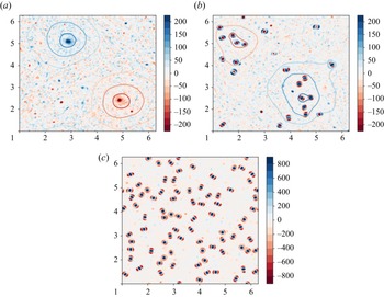
Figure 1 shows snapshots of typical solutions at different $\gamma$ obtained by integrating from small-amplitude random initial conditions. At $\gamma =0$ (random forcing) a large-scale condensate forms. At $\gamma =0.35$ a large-scale circulation persists, as indicated by the streamfunction, but small tripolar vortices with positive and negative cores appear, concentrating within the large-scale vortices of the corresponding sign. We stress that the large-scale vortices evolve in time, constantly changing their position and shape. 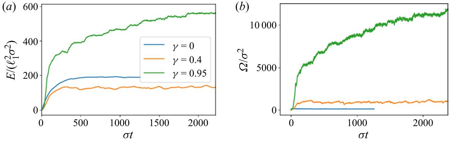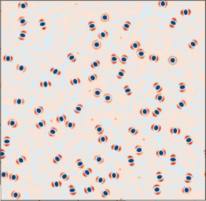At $\gamma =1$ a state of broken symmetry is present, with a large number of same sign vortices. We call this state a (shielded) vortex gas. In our runs with regular viscosity, we observed the same phenomenology as in figure 1. In figure 2, we show the time evolution of energy and enstrophy for each of the three observed regimes. When a condensate is present, energy and enstrophy saturate quickly, but continue to grow in the case of the vortex gas. This case is discussed in much greater detail in § 5.

Figure 1.

Visualisations of the vorticity field, with contour lines showing the streamfunction (a,b only). (a) Large-scale condensate state at $\gamma =0$. (b) Mixed state, with SVs clustering in large-scale vortices at $\gamma =0.35$. (c) Dilute gas of SVs at $\gamma =1$. Note the different colour scale used in (c).

Figure 2.

Time series of non-dimensionalised energy $E$ and enstrophy $\varOmega$ for a condensate state ($\gamma =0$), a mixed state ($\gamma =0.4$) and SV gas ($\gamma =0.95$). For the former two cases, a steady state is reached quickly, while in the vortex gas, energy and enstrophy grow slowly.

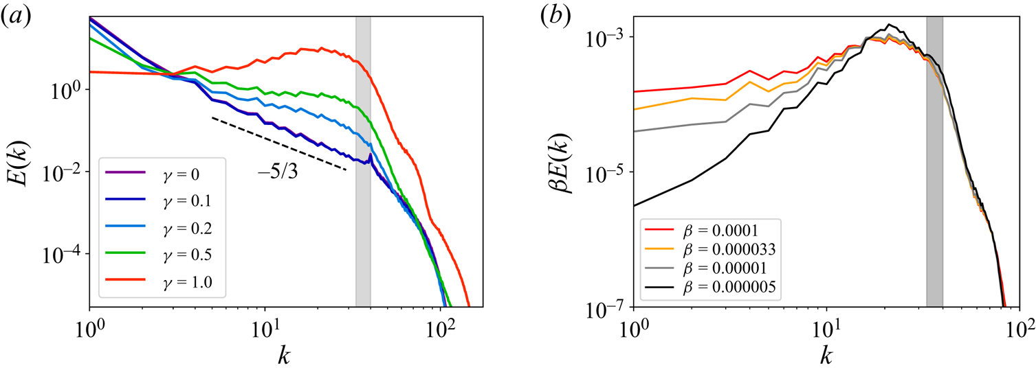
The spectra associated with states at different $\gamma$ are shown in figure 3(a). At $\gamma =0$ and $\gamma =0.1$, there is a $-5/3$ power-law range at scales larger than the forcing, and a build-up of energy at $k=1$, i.e. a condensate. As $\gamma$ increases through $0.2$, the energy in the large scales decreases and that in the near-forcing scales increases, marking the appearance of SVs. The condensate is weaker but persists at $\gamma =0.5$, while the near-forcing-scale energy grows. Finally, at $\gamma =1$ the spectrum no longer peaks at the largest scales, but rather at scales comparable to twice the forcing scale $\ell _1\equiv 2{\rm \pi} /k_1$. The spectral bumps seen at high $k$ are likely related to harmonics of the main peak. Figure 3(b) shows the spectrum in the vortex gas state ($\gamma =0.9$) at different values of the damping coefficient $\beta$, rescaled by $\beta$. At the forcing scales and below, the rescaled curves collapse. At smaller $k$, as $\beta$ decreases, the peak near $2\ell _1$ becomes more pronounced, and the portion of energy in large scales falls, due to larger vortex amplitudes at smaller $\beta$.

Figure 3.

Energy spectra $E(k)$ at late times, averaged over the last 500 snapshots. The grey bar indicates the forcing range $[k_1, k_2]$. Dashed line indicates a $-5/3$ power law. (a) Spectra for different $\gamma$ from set A. The same colour scale used here for different $\gamma$ is used subsequently in figures 4, 5, 8. (b) Spectra for different $\beta$ ($\gamma =0.9$, set C), scaled by $\beta$.

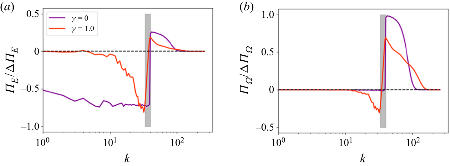
Figure 4 shows the energy and enstrophy fluxes at $\gamma =0$ (random forcing) and $\gamma =1$ (vortex gas). The negative (i.e. inverse) energy flux in the vortex gas state is suppressed at scales larger than approximately $2\ell _1$. A small forward energy flux feeds the remaining finite dissipation at small scales. The forward enstrophy flux for random forcing remains so in the vortex gas although a small inverse enstrophy flux is also present, reaching to around $k_1/2$. We stress that residual fluxes at $\gamma =1$ are strongly scale-dependent, indicating absence of self-similar cascade, in contrast to the $\gamma =0$ case where fluxes are reasonably constant. The suppression of nonlinear transfers by coherent vortices is reminiscent of that in decaying 2-D turbulence (McWilliams Reference McWilliams1984). In our case, there are two competing time scales, however: the instability growth rate at which energy is injected into the forcing scales, and the rate at which energy is transferred out of the forcing scales by nonlinearity. If energy is injected too rapidly for nonlinear transfer to remove it, it builds up near the forcing scales, and coherent vortices form, further suppressing nonlinear fluxes. In the absence of any cascade mechanism, nonlinear damping is required to saturate the build-up of near-forcing-scale energy.

Figure 4.

(a) Energy flux $\varPi _E$ and (b) enstrophy flux $\varPi _\varOmega$, rescaled by ${\rm \Delta} \varPi _i = \max _{k}(\varPi _i)-\min _k(\varPi _i)$, $i=E,\varOmega$, averaged over 500 time steps at late times, for $\gamma =0$ (random forcing), and $\gamma =1$ (vortex gas). Unrescaled fluxes in the gas are significantly greater than at $\gamma =0$ and fluxes are strongly scale-dependent: $\varPi _E$ is suppressed at large scales, while $\varPi _\varOmega$ is forward, with a weak local inverse transfer. Shaded region indicates forcing.

4. Vorticity statistics and radial profiles

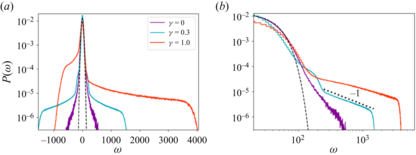
The spectra and fluxes of inviscid invariants are useful tools for analysing turbulence but have two shortcomings. First, spectral studies discard phase information and in particular vortex signs. Second, in the presence of coherent structures, such studies do not provide us with the corresponding physical space picture. To address these points, we begin by considering the statistics of the signed vorticity. Figure 5 shows the probability density function (PDF) of vorticity, $P(\omega )$, for three different values of $\gamma$ from set A, generated from over 800 snapshots. At $\gamma =0$ (random forcing) the central region of the PDF near $\omega =0$ is close to a Gaussian, but there are heavy tails at larger $|\omega |$. This is consistent with the results of Pasquero & Falkovich (Reference Pasquero and Falkovich2002). For $\gamma =0.3$, the SVs that are present manifest themselves in the form of significantly longer heavy tails in the PDF, but the PDF remains approximately symmetric. At $\gamma =1$, the amplitude of the SVs extends to larger $|\omega |$ due to stronger driving, and a pronounced skewness in the PDF develops, reflecting the broken symmetry. 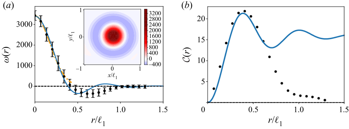The log–log plot in figure 5 shows that the heavy tails are of power-law form with exponent close to $-1$. Power-law tailed PDFs can correspond to rare events in time or in space. Here, they represent the spatial localisation of vorticity inside SVs, which are coherent over long times. Figure 6(a) shows the radial vorticity profile within the SVs, computed in the vortex gas. The profile is averaged over many vortices with arbitrary orientation, resulting in an effective azimuthal average. A nearly Gaussian core is surrounded by a shield of opposite-sign vorticity, with $|\omega |=0$ at $r\approx 2{\rm \pi} /k_1\equiv \ell _1$, i.e. the largest forcing scale. In addition to the Gaussian profile, we also compare the vorticity profile to the theoretical result of Jiménez (Reference Jiménez1994) for hyperviscous vortices, which also predicts a sign change in vorticity with radius, not unlike what we observe here. However, figure 5(b) shows that the circulation $\mathcal {C}$ associated with the vortices in our DNS vanishes beyond $r\geq \ell _1$. Since $\mathcal {C}=2{\rm \pi} \int _0^r \omega (r) r\,{\rm d} r = \int _{\mathcal {C}(r)} \boldsymbol {u}\boldsymbol {\cdot } {\rm d}\mathcal {\ell }$, the vanishing of $\mathcal {C}(r)$ indicates that the vortices do not generate a velocity outside this radius, and that they are thus well shielded. In contrast, the hyperviscous vortices of Jiménez (Reference Jiménez1994) are not shielded since their circulation tends to a non-zero constant as $r$ increases. For a Gaussian profile $\omega (r)$, the near circular symmetry of the core $P(\omega )\,{\rm d}\omega \propto 2{\rm \pi} r \,{\rm d} r$ implies, in approximate agreement with figure 5,

(4.1)\begin{equation} P(\omega) \propto 2{\rm \pi} r(\omega)/({\rm d}\omega(r)/{\rm d} r)|_{r=r(\omega)} \propto \omega^{{-}1}. \end{equation}

We have also computed the radial vorticity profile in SVs for the runs in set D, with regular viscosity (hyperviscous exponent $n=1$) and find qualitatively the same fully shielded profiles, with the vortex size set by $\ell _1$ as in the hyperviscous runs. This indicates that the shielding is not an artefact of hyperviscosity, but rather an intrinsic result of the nonlinear dynamics.

Figure 5.

(a) Lin–log plot of the vorticity PDF sampled over all spatial points, aggregated over 800 snapshots, for three different values of $\gamma$ from set A. The dashed curve centred on $\omega =0$ is a Gaussian fit. (b) Same quantities in a log–log plot. The tails have power-law form: the thick dashed line shows a power law with exponent $-1$.

Figure 6.

(a) Circles: average SV profile at $\gamma =0.9$ (set A). Approximately Gaussian core (orange dash-dot line, Gaussian fit; blue solid line, hyperviscous prediction from Jiménez (Reference Jiménez1994) with hyperviscosity exponent $n=4$ as used here) surrounded by an opposite-signed shield. Radial extent is set by $\ell _1\equiv 2{\rm \pi} /k_1$. Inset: population average over many tripolar vortices with arbitrary orientations. (b) Circulation $\mathcal {C}(r) = 2{\rm \pi} \int _0^r \omega (r') r' \,{\rm d} r'$ for an average SV (black circles) becomes vanishingly small beyond $r\gtrsim \ell _1$, indicating vanishing azimuthal velocity and no long-range interactions. Blue solid line, as in (a).

5. Spontaneous symmetry breaking and vortex census

As mentioned, SVs of one core sign appear in the flow at late times, provided the instability growth rate is large enough. Rotating turbulence also displays cyclone–anticyclone asymmetry (Bartello, Métais & Lesieur Reference Bartello, Métais and Lesieur1994) but this asymmetry is the result of forced symmetry breaking. 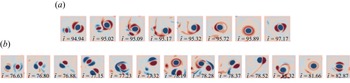Here, the flow maintains approximate symmetry in $\omega$ as it develops from unbiased small-amplitude initial conditions, but if $\gamma$ is large enough, this transient leads to a symmetry-broken phase where one or other sign dominates. To understand the physical space processes enabling symmetry breaking, we highlight in figure 7 two examples of typical interactions in this phase between opposite-signed SVs (for $\gamma =0.9$). In figure 7(a), a stronger vortex encounters a weaker one. The latter is stripped of its shield, undergoes shearing, and merges with the shield of the stronger vortex. A circular shield forms ($\tilde {t}=95.89$), which then breaks up into a tripolar one ($\tilde {t}=97.17$) as seen in experiments (Kloosterziel & Van Heijst Reference Kloosterziel and Van Heijst1991). The interaction described above is part of the symmetry-breaking process: from random small-amplitude initial conditions emerges a sea of vortices of both signs. Statistically, the populations are equal, but due to fluctuations, some vortices are stronger than their nearby opposite-signed counterparts. The interaction then eliminates the weaker vortices near stronger ones, and thus leads to a population imbalance. Asymmetric interactions are more likely at large $\gamma$, due to larger differences in the strength of vortices born at different times.

Figure 7.

(a) Absorption of a weak SV into the shield of a stronger one of opposite sign. (b) Life cycle of a dipole born from two colliding SVs of similar strength. In both cases $\gamma =0.9$. Time is given in terms of $\tilde {t}=\sigma t$. Colours show vorticity (blue positive, red negative).

The above scenario presumes an asymmetry between interacting vortices. Figure 7(b) shows a typical scenario ensuing when the vortices have comparable amplitudes: both vortices are stripped of their shields, forming a propagating dipole pair, cf. Jiménez (Reference Jiménez2020). At $\tilde {t}=77.15$, the dipole encounters a SV with a negative core, and the resulting collision strengthens the negative vortex, leading to an asymmetric dipole at $\tilde {t}=77.32$ whose curved trajectory results in a collision with a SV with a positive core at $\tilde {t}=78.19$. The result is again an asymmetric dipole, but this time with a dominant positive vortex. Note that after each collision the dominant component is determined by the core of the target vortex. In a subsequent interaction the dipole shears out the subdominant vortex into a shield around the positive core, finally becoming tripolar. The process of dipole formation, collisions and return to a single SV does not a priori favour either vortex sign. However, due to the asymmetric interaction described earlier, vortices of one sign may become more numerous. Thus, dipoles are more likely to collide with vortices of the dominant sign, thereby reinforcing their dominance.

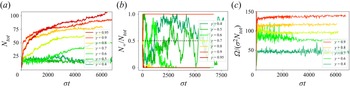
To track the vortex population, we perform a census. For this we exploit the fact that saturated SVs differ only weakly in strength, cf. figure 1. We thus filter the vorticity field, setting to zero any values with magnitude below a threshold of 75 % of the maximum vorticity magnitude (we verified that the result is insensitive to the precise choice of this threshold). Finally, we apply a maximum filter at the scale of vortex cores to determine the position of all vortices at a given instant. Figure 8 shows the total number of vortices $N_{tot}$ and the fraction of positive vortices vs time for different $\gamma$.

Figure 8.

Vortex census data obtained as described in the text. (a) Total number of vortices $N_{tot}$ vs. time for different $\gamma$. (b) Fraction of $+$ vortices vs time. (c) Enstrophy per vortex.

Figure 8(a) shows that for $\gamma <0.6$, the number of vortices fluctuates around $N_{tot}\approx 20$, and does not show any increasing trend. The flow field for these runs resembles that in figure 1(b). There the positive/negative vortices are physically separated, since they cluster inside large-scale vortices of the same sign. For all runs at $\gamma \geq 0.6$, however, $N_{tot}$ increases with time. The larger $\gamma$, i.e. the larger the growth rate, the more rapid is this increase. Despite the long integration time of $\sigma t\lesssim O(10^4)$, $N_{tot}$ continues to slowly drift. The moderate resolution allows us to discern this slow trend. The increase is due to random nucleation events occurring in the sea of turbulence between vortices, which requires a vortex seed to mature without being disrupted by shear. This is likely why $N_{tot}$ rises faster at larger $\gamma$: vortices reach large amplitudes more rapidly and are harder to disrupt.

Figure 8(b) shows the fraction of vortices with positive core vs time for different $\gamma$. At $\gamma <0.6$, this quantity fluctuates between $0$ and $1$, without converging to any particular value. At $\gamma =0.6$, a long transient, $\sigma t\sim 3000$, leads to a state of only negative vortices. At larger $\gamma$, the elimination of vortices with one sign is more rapid, but the emergent dominant sign is random. We quantify this transition by the enstrophy $\varOmega$ defined earlier. The enstrophy per vortex saturates quickly, and subsequently remains constant in time and increases with $\gamma$ (see figure 8c). There is a striking separation between the fast saturation in the amplitude of individual vortices, and the slow nucleation of new vortices.

6. Multistability

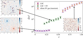
Figure 9 summarises the transitions between the different states shown in figure 1, as a function of $\gamma$, in terms of the late-time enstrophy $\bar {\varOmega }$. At small $\gamma \leq 0.30$, the large-scale condensate (LSC) state exists, without any coherent SVs. For $\gamma < 0.2$, the LSC states form spontaneously from small initial conditions (set A). At $0.2\leq \gamma \leq 0.3$, LSC states are stable when the flow is initialised in an LSC state (set B), but the system does not spontaneously form an LSC from small initial conditions. For $0.2\leq \gamma \leq 0.55$, one observes an LSC with coherent vortices of both signs, as shown in figure 1(b). Over the range $0.2\leq \gamma \leq 0.3$, there is bistability between LSC states with and without SVs. For yet larger growth rates $\gamma \geq 0.6$, a state of broken symmetry forms from all initial conditions investigated. As described in the previous section, in this regime the number of vortices $N_{tot}$ steadily grows and figure 9 therefore shows the enstrophy at the end of each simulation. We expect that $N_{tot}$ will keep growing until a high-density, potentially crystalline, state is reached. A detailed study of this saturation process and of the final steady state requires very long simulations, and merits a separate study.

Figure 9.

Summary of states at different $\gamma$ in terms of the mean enstrophy (error bars indicate standard deviation). For $\gamma \leq 0.3$, a large-scale condensate (LSC) is observed. The LSC states at $0.2,0.25,0.3$ are from set $B$. Mixed states, where an LSC coexists with SVs of both signs, are seen for $0.2\leq \gamma \leq 0.55$. Symmetry breaking occurs for $\gamma \geq 0.6$.

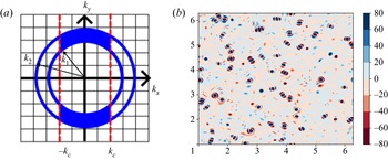
Given the rich state space shown in figure 9, one may ask to what extent the results described here are specific to the choice of forcing we employed. To address this, we first tested different widths of the forcing range by varying $k_1,k_2$. For a given domain size, when $k_1$ is close to $k_2$, the discrete Fourier grid generates an underlying anisotropy. The dynamics in this limit are not very relevant physically, since they originate in the numerical discretisation alone. When the wavenumber shell is widened, this anisotropy disappears. In this regime, we always observe SVs, provided the instability forcing is sufficiently strong. This remains so when the dispersion relation (2.3) is modified to a top-hat profile. In addition, we considered anisotropic forcing, illustrated in figure 11, obtained by truncating the annulus $k_1\leq |\boldsymbol {k}|\leq k_2$ of instability-forced wavenumbers $\boldsymbol {k}=(k_x,k_y)$ by requiring that $k_x$ be below some cutoff wavenumber $k_c$ chosen such that $k_c< k_1$, and observed both SVs and symmetry breaking for all values of $k_c$ that we considered. 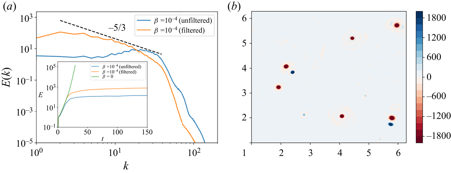We also repeated the runs in set $A$ with a modified random forcing $\boldsymbol {f}_\epsilon$ acting on the same scales $[k_1,k_2]$ as the instability (instead of a thin shell centred on $k_2$) and observed the same transitions as shown in figure 9 at approximately the same $\gamma$. We conclude that our qualitative results are robust to changes in the details of the forcing. In addition to varying the forcing, one can also investigate the impact of nonlinear dissipation in our model. The dissipation acts on all scales, but the forcing is spectrally localised. To test whether this is relevant, we performed DNS where the nonlinear dissipation is filtered in Fourier space so it only acts on the forcing scales $[k_1,k_2]$. In this case, we find that the inverse energy cascade is no longer suppressed, as evidenced by the energy spectrum shown in figure 10. Figure 10(b) shows the corresponding vorticity field. Shielded vortices appear at early times, but the shields are subsequently lost, and do not suppress the inverse cascade. This experiment tells us that nonlinear dissipation that acts on all scales larger than the forcing scale is crucial for suppressing the inverse cascade, by dissipating energy efficiently and keeping it from reaching large scales. However, the suppression of the inverse cascade remains spontaneous, since an inverse cascade persists for random forcing, and only disappears for strong instability-type forcing. We mention, finally, that multistability occurs in quasi-2-D turbulence (Favier, Guervilly & Knobloch Reference Favier, Guervilly and Knobloch2019; van Kan, Nemoto & Alexakis Reference van Kan, Nemoto and Alexakis2019) and beyond (Ravelet et al. Reference Ravelet, Marié, Chiffaudel and Daviaud2004) although we observed no spontaneous transitions between different branches.

Figure 10.

(a) Spectra for nonlinear damping $\beta |\boldsymbol {u}|^2 \boldsymbol {u}$ either full or filtered in Fourier space to be non-zero only within the forcing range. (b) Vorticity field at long time for the filtered case. Inverse energy transfer occurs when nonlinear dissipation is filtered, but is suppressed otherwise, indicating that the damping plays an important role in the suppression.