2. EDGEWORTH EXPANSIONS UNDER INEQUALITY RESTRICTIONS

Suppose that

are the unknown parameters that are subject to some inequality constraints. We write the constraints as

for some p ≤ n, where the functions g_j(.) are known. In vector notation we can write g(θ) ≥ 0. There may also be strict inequality restrictions and equality restrictions, but we shall not separately formalize these for notational simplicity. Each restriction g_j implies a subset Θ_j of

, and collectively the parameter space becomes Θ = ∩_j=1^pΘ_j. A leading example is where θ_j ≥ 0, j = 1,…,p, in which case

. Other examples such as

are more complicated but fall under the general case laid out previously.

We suppose that there is an objective function l_T(θ) that depends on the data. Maximization of l_T(θ) over the (restricted) parameter space yields the estimator θ* = (θ₁*,θ₂*,…,θ_n*) that we analyze here. Let

be the unrestricted estimator that maximizes l_T(θ) over

. The estimator objective function can be the log-likelihood, the quasi log-likelihood, a least squares criterion function, a generalized method of moments (GMM) objective function, a minimum distance objective function, an objective function that depends on finite- or infinite-dimensional preliminary estimators, etc. (for more details, see Andrews, 1999). By definition, the extremum estimators θ*,

satisfy

Our approach to solving the inequality constrained optimization problem is to look at all the subcases where one or more of the restrictions are binding; see Otten and Bams (2001). Suppose that g_j1(θ) = 0,…,g_jr(θ) = 0 for some r and some {j₁,…,j_r}; then we have a standard equality constrained optimization problem

which can be solved by standard methods. We search over all such subcases and then find the parameter value that satisfies all inequality restrictions and that maximizes the criterion. In general there are (2^p − 1) possible restricted problems to consider, which means that we can get

possible estimators subject to binding restrictions. Then the estimator over the set Θ, denoted θ* = (θ₁*,θ₂*,…,θ_n*), is whichever of

satisfies the estimation criterion (the objective function is optimized) and the restrictions. There is a natural specific to general strategy that should be adopted here: start with the unrestricted problem; if the solution value satisfies all the inequality restrictions then stop. Then look at each of the r = 1 subproblems and check whether any of their solution values satisfies all the inequality restrictions. If at least one does, then one can stop and take whichever solution value maximizes l_T(θ). One proceeds through r = 1,…,p until a solution is found.

, i.e., θ* = g(Z_T) for some g. Therefore, if the distribution of Z_T is known or can be approximated by some signed measure and if the mapping g is well behaved, then the distribution of θ* or an approximation to it can be obtained by some manipulations. We will deal with cases where both of these conditions are met.

An important ingredient in our approximation is going to be the approximation to the distribution of Z_T. Consider a general vector

of standardized estimators that is asymptotically normal with variance matrix Ω and satisfies a joint Edgeworth expansion. Suppose that the first three mixed cumulants of Z_T satisfy

for arrays of constants {c_i}_i=1^d, {c_ij}_i,j=1^d, {c_ijk}_i,j,k=1^d. Then for any Borel set B,

where

The quantities H_i(y) and H_ijk(y) are the multivariate Hermite polynomials of first and third degree. See Taniguchi and Kakizawa (2000, p. 170) and Barndorff-Nielsen and Cox (1989, p. 174).³

In some special cases the calculations involved simplify considerably. Specifically, when the restrictions are “nested” one can dispense with the likelihood functions in Z_T. Suppose that for each r = 1,…,p there is only one case; then one does not need to know the likelihood function value to conclude which value to take as there is a natural ordering just based on r. A trivial example is when there is only one restriction, such as the ARCH(1) process, but the GARCH(1,1) model is also of this type. In Section 3 we discuss these two examples in detail.

3. EXAMPLES

3.1. ARCH(1) Process

Suppose that

where ε_t is independent and identically distributed (i.i.d.) with mean zero and variance one, and let

be the unknown parameters. We suppose that θ₁ > 0 and θ₃ ≥ 0 (nonnegativity constraint).

⁴

The case of weak stationarity where θ₃ ≤ 1 can be treated identically.

The constraint that θ₁ > 0 precludes the possibility that θ₁ = 0 and so can never be binding. Let

be the restricted parameter space. Let

be the unrestricted QMLE, i.e., the maximizer over

of the quasi log-likelihood. Let

be the maximizer subject to the binding restriction that θ₃ = 0. Then the maximizer over the set Θ, denoted θ*, is whichever of

makes the likelihood bigger and satisfies the restrictions. This is a nested case because

, and so all that is required is to check whether

satisfies the restrictions. Thus θ* is a mixture of the two parameters

These equations represent the inequality restricted estimator θ* in terms of two equality restricted estimators

. Thus the joint distribution of

determines the distribution of θ*. In particular, by the law of total probability (conditioning on the event

and its complement),

To approximate Pr[θ₃* ≤ x] we only need the marginal Edgeworth expansion for the estimator

, and this calculation is standard; see Linton (1997).

⁵

This approximation can be justified by the results of Götze and Hipp (1983) under conditions on the parameters that ensure that the process is stationary and strong mixing with geometric decay.

If θ is in the strict interior of the parameter space the probabilities like

increase exponentially to one, and the standard expansion applies to Pr[θ₁* ≤ x]. But when, e.g., θ₃ = 0 this probability converges at a more modest pace to one-half. That expansion is no longer valid, and we must compute the more complicated expression given in (8). Therefore, in general to approximate Pr[θ₁* ≤ x] we need to approximate

and

, which require the joint asymptotic expansions of

and of

. The calculations involved in obtaining the joint asymptotic expansion are quite similar to those for the marginal expansions and are discussed further in the Appendix.

Suppose that we have approximations Ψ_Tj, j = 0,1,2 (as described in (5)), such that

Then let Ψ_T3*(x) = Ψ_T0(x) and

for x ≥ 0 and Ψ_T1*(x),Ψ_T3*(x) = 0 otherwise. It follows that Ψ_Tj*(x) are valid approximations to Pr[θ_j* ≤ x] in the sense that

This is true for all values of θ including the boundary ones.

To compute the approximate bias or skewness one can use and integrate the approximating measure. For example, an approximation to the bias of θ₁* is given by

; see Section 3.2.

To apply this general formula one just has to take different vectors Z_T and Borel sets B in (5). To compute Pr[θ₁* ≤ x] we need to apply (5) to the cases

and

. We also need to compute the probabilities

using the univariate Edgeworth expansion.

3.2. GARCH(1,1)

Suppose that

where ε_t is i.i.d. with mean zero and variance one. Let

be the unknown parameters where θ₁ > 0 and θ₂ ≥ 0, θ₃ ≥ 0 (but if θ₂ = 0, then θ₃ = 0). Because of this last qualification this is a nested case, and the restrictions are (we ignore the restriction that θ₁ > 0)

This is exactly the situation described in Jensen and Rahbek (2004a, 2004b), where the authors need the parameters to be positive. Let

be the unrestricted QMLE (other estimators may be analyzed using the same methodology), i.e., the maximizer over

of the quasi log-likelihood. Let

be the maximizer subject to the binding restriction that θ₂ = 0 and let

be the maximizer subject to the binding restrictions that θ₂ = 0 and θ₃ = 0. Then the maximizer over the set Θ, denoted θ*, is whichever of

makes the likelihood bigger and satisfies the restrictions. Clearly,

, and so it amounts to just checking first whether

satisfies the restrictions, if not then checking whether

satisfies the remaining restrictions, etc. Thus θ* is a mixture of the three parameters. In fact

A consequence of (11)–(13) is that

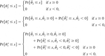
We apply the same methodology as in the ARCH case.

4. INFERENCE AND BIAS CORRECTION

The preceding approximate distributions can be used when the parameters θ are known, say, under a null hypothesis. We now discuss how our expansions can be used for inference. The main issue here is that our distributional approximations are discontinuous in the parameters, e.g., Ψ_T3*(x;θ) is not (uniformly) continuous in θ. This is of no consequence if the parameters are known, but when the parameters are unknown this complicates matters. For example, the natural estimator of the distribution

does not well approximate Ψ_Tj*(x;θ) when θ is on the boundary of the parameter space. This is why the standard inference methods do not apply. It follows that the obvious bias correction methods also do not work as usual. We argue that by using an alternative estimator of θ in Ψ_Tj*(x;θ) one can obtain consistency. We focus on the bias correction issue for simplicity and present the main ideas for the case of the parameter θ₃ in the ARCH model.

From (5), the density of

is approximately (to o(T⁻¹))

where ω is the asymptotic variance of

, whereas h₃,h₃₃₃ are the one order higher Hermite polynomials corresponding to H₃,H₃₃₃; see Rothenberg (1984, (3.3)). Actually, h₃(x) = 1 and h₃₃₃(x) = x³ − 3x. Therefore,

This approximation is valid to order T⁻¹, and the left-hand side is interpreted as an asymptotic moment because the actual moment may not exist. See Srinivasan (1970) for related discussion. We next specialize this general formula in the two cases.

When θ₃ = 0, we have

because

. When θ₃ > 0

Thus when θ₃ > 0 the bias is of order T⁻¹, whereas when θ₃ = 0, the bias is larger and of order T^−1/2 with a second-order term of order T⁻¹.

To use this for bias correction one should replace the bias b_T(θ) by the estimated bias

where ω* = ω(θ*), c₃* = c₃(θ*), and c₃₃₃* = c₃₃₃(θ*). Unfortunately, this does not work when the parameter is on the boundary; specifically,

converges to a random limit in that case (because

has a nondegenerate limiting distribution). Instead we shall follow Andrews (2000) and work with a modified estimator that avoids this problem.

and define

Then define the estimated bias b_T(θ**) as in (15). It can be shown that

for all θ₃ ≥ 0. The reason for this is that when θ₃ = 0,

for any r > 0 because

. Therefore

and similarly for the other terms. When θ₃ > 0, b_T(θ) = O(T⁻¹), and the estimated version b_T(θ**) is of smaller order in probability. It follows that the additive and two alternative multiplicative bias corrected estimators θ_abc* = θ* − b_T(θ**), θ_mbc1* = θ*/(1 + b_T(θ**)/θ*), and θ_mbc2* = θ* exp(−b_T(θ**)/θ*) (where 0/0 = 0) have bias of order o(T⁻¹). The exponential bias corrected estimator may be preferred because it is always nonnegative, whereas the additive bias corrected estimator can be negative and hence violates the restrictions we seek to impose.

The generalization of the bias correction mechanism to the multidimensional case implies retrieving the bias function b_T(.) from (5) and again using a modified estimator to apply in (16). For example, in the GARCH(1,1) case where we impose the positiveness constraint in all the parameters and again using the notation of Section 3, we define the bias correction using the shrinkage estimates:

,

, and

.

In conclusion, we have shown how to correct the constrained estimator for bias, first and second order. Our method is based on analytical calculations and use of the shrinkage estimator θ**. An alternative would be the bootstrap methods proposed in Andrews (2000). Our approach works also for distributional approximation, so that Ψ_Tj*(x;θ**) approximates Ψ_Tj*(x;θ) to the required order uniformly over x. Note however that as in Andrews (2000) the result (16) is a pointwise result and does not extend to uniformity, e.g., to the sequence of true parameters converging to zero.

5. SIMULATIONS

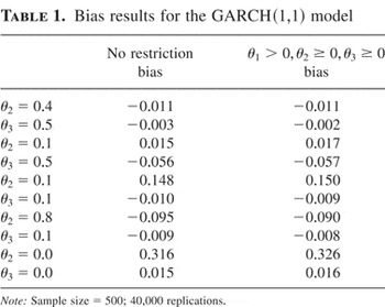
We now present simulation results to analyze the consequences of imposing restrictions in the GARCH(1,1) model and later also in the ARCH(1) model. Table 1 shows the results for 40,000 replications with a sample size of 500 observations, and it shows the bias of the estimates both when we restrict and when we do not restrict the parameter space to be in the positive region in the GARCH(1,1) model; ε_t ∼ N(0,1). We show the bias results without and with the positiveness restrictions when estimating by QML for the (θ₂,θ₃) parameter values equal to (0.4,0.5), (0.1,0.5), (0.1,0.1), (0.8,0.1), (0.0,0.0). The biases are free of the value of θ₁, which has been set to 0.81 in all simulations.

value is large, while

is small, and so it is important that the researcher be aware that mainly this situation is the one that is very likely to generate relatively large biases. The biases are especially large when both θ₂ and θ₃ are small. The restriction of positiveness slightly increases the bias in general, although less than happens for the ARCH(1) model (as we will see in the next section). The results clearly justify that, both when restrictions are imposed and when they are not, the estimates need a bias correction mechanism in practice. When the true parameter value is on the boundary, the bias increases significantly mainly for

.

Bias results for the GARCH(1,1) model

If we are only interested in correcting the first-order bias, e.g., if the restriction is the positiveness of the parameter space, the first-order bias term (in a standardized case) is simply given by E(max(Z,0)) for Z ∼ N(0,1) (according to the theory of Andrews, 1999), whereas if the restriction is to impose that the parameter space is less than 1, then the first-order bias is given by E(min(Z,1)) for Z ∼ N(0,1). However, to consider the second-order bias, we need to apply the theory developed in Section 2 to the GARCH(1,1) and the ARCH(1) models. This is done in the Appendix.

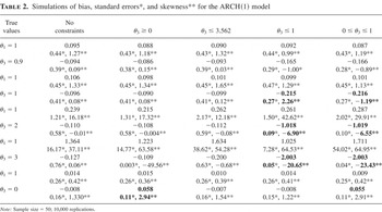
We present in Table 2 simulation results to find out about the consequences of imposing restrictions in the estimation of an ARCH(1) model. Table 2 presents results for the bias; with an asterisk, we also provide the standard errors of the estimators, and with a double asterisk we show the skewness. We present the results in five different scenarios: when we do not restrict the estimator, constraining θ₃ ≥ 0, constraining θ₃ ≤ 3.562 (strict-stationarity condition in the ARCH(1) model), constraining θ₃ ≤ 1 (weak stationarity), and 0 ≤ θ₃ ≤ 1. We show the results for different combinations of true values: (θ₁,θ₃) = (1,0.9), (θ₁,θ₃) = (1,1), (θ₁,θ₃) = (1,2), (θ₁,θ₃) = (1,3), and (θ₁,θ₃) = (1,0). In this way we analyze the behavior of the ARCH(1) model in both the stationary and nonstationary regions (see Jensen and Rahbek, 2004a, 2004b, where they prove that the QMLE is still consistent and asymptotically normal in the nonstationary area) and also when a restriction is binding or not.

Simulations of bias, standard errors*, and skewness** for the ARCH(1) model

If the true parameter value is 0.9, the fact of having a bias of −0.17 (when we constrain 0 ≤ θ₃ ≤ 1) is an important problem (when the researcher estimates with that constraint in practice), and therefore, to bias correct is quite relevant. In the same way, when θ₃ = 2, to impose the weak stationarity constraint wrongly can have very important consequences. It is true that under restrictions, the standard error is reduced (as is shown in Table 2), although we have to judge that together with the fact that the bias in the restricted estimator is amazingly large. In summary, restrictions can affect significantly the estimates in this context. We also show in bold the behavior of the skewness, the standard errors, and the biases when the restrictions are binding. In Table 2, we show that the biases can increase very significantly: e.g., when the true θ₃ = 1 and we impose the constraint of 0 ≤ θ₃ ≤ 1, the bias reaches the value −0.216 (it is a bias of around 20% of the true parameter value). Also, the skewness increases very significantly when the true parameter touches the boundary of the restriction. Finally, we also show how the variance of the θ₁ estimator increases significantly when restrictions are imposed in the estimation of θ₃ and when we are in the nonstationary area.

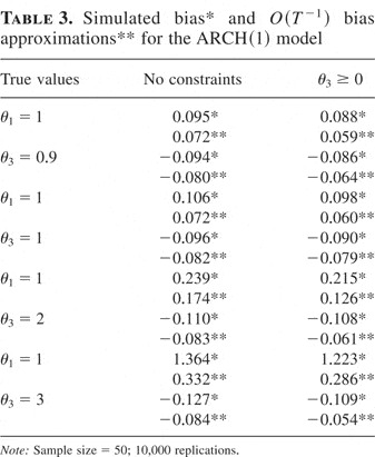
Now that we know from Tables 1 and 2 how the restrictions can affect the bias, standard error, and skewness of the estimators, we want to find out how our theory is able to correct for the problem. In Table 3, we show the simulated second-order bias of the estimator with one asterisk, and with a double asterisk we show the value that our theory predicts and that should match the second- order bias of the estimator. Note that for the bias of

and

we use the expressions of the bias given in the Appendix in equation (A.2). Because the bias expressions in the ARCH(1) model involve summations from 1 up to the sample size, we follow the recommendation in Iglesias and Phillips (2005), where it is shown that if we truncate those summations in 8, they already provide a very good approximation of the true bias. Our theory explains and predicts the movement of the true second-order bias, and it accounts for an important portion of its amount (see Table 3) mainly for

. We consider again the estimates under no constraints and with the positiveness constraint under (θ₁,θ₃) parameter values equal to (1,0.9), (1,1), (1,2), (1,3). We show that it is especially interesting how when the true value of θ₃ = 1, without the bias correction mechanism (because of the heavy downward bias of −0.09) we would conclude that the disturbance is weakly stationary, whereas in fact it contains a unit root. That means that using only asymptotic theory can have dangerous consequences in the interpretation of the estimates in some circumstances.

Simulated bias* and O(T−1) bias approximations** for the ARCH(1) model

Finally, in Table 4 we show the simulated first-order bias of the estimator (what the theory of Andrews, 1999, predicts) and the total bias when the parameter is on a boundary. The design of the experiment includes the (θ₁,θ₃) parameter values equal to (1,0), (1,1). We find that for some restrictions, the Andrews (1999) theory provides a very good approximation (when the restriction is θ₃ ≥ 0), whereas for another restriction (for imposing weak stationarity such that θ₃ ≤ 1), the first-order approximation again in a standardized case (coming from E(min(Z,1)) where Z ∼ N(0,1)) is not very accurate, and higher order refinements are very advisable. We also show the total simulated skewness and the first-order approximation for the skewness that the Andrews (1999) theory would predict. The skewness term comes in the first case of Table 4 from the term E[(max(Z,0) − E(max(Z,0)))³]; and for the second restriction from E[(min(Z,1) − E(min(Z,1)))³]. We see that the first-order asymptotic theory for the skewness does not offer a good approximation in the case of the first restriction or for the second one.

First-order bias, total simulated bias*, first-order skewness**, and total simulated skewness*** for the ARCH(1) model

5.1. Inference and Bias Correction

We proceed now to show in practice how our procedure of Section 4 corrects the constrained estimator for bias, first and second order. As we have pointed out, our method is based on analytical calculations and use of the shrinkage estimator θ**. We consider the setting of an ARCH(1) process in (6), with a sample size of 50 observations and 10,000 replications; ε_t ∼ N(0,1). We show the results of our uncorrected and bias corrected estimators using robust estimates in terms of median and interquartile range (because the approximations are valid in probability). We also consider two restrictions that the applied researcher may consider in practice: (1) a positiveness constraint and (2) a constraint to impose a finite unconditional variance.

If we are in a setting where θ₁ = 1 and θ₃ = 0, and we estimate subject to the constraint

then the uncorrected estimator θ₃* has a bias (see Table 2) of 0.058 and a standard error of 0.111. Therefore, we consider a shrinkage estimator, θ₃**, that we use for bias correction of θ₃*:

where, for η_T, we have used a rate of T^−1/4 and scaled by the square root of the variance of the unrestricted estimator. Therefore, following our methodology in Section 4, we construct three types of bias corrected estimators of θ₃*: θ_3,abc*, θ_3,mbc1*, and θ_3,mbc2*.

We repeated the same experiment with the second constraint where now θ₁ = θ₃ = 1 and

The bias and standard error of θ₃* (see Table 2) are −0.215 and 0.269, respectively. We construct again a shrinkage estimator of the type

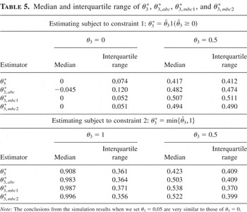
and we obtain the three bias corrected estimators. Table 5 shows the median and interquartile range of θ₃* (the uncorrected estimator) and the three bias corrected estimators under the two constraints. We can observe how under constraint 1, the additive bias corrected estimator can reach negative values and therefore it distorts its median and interquartile range in relation to the uncorrected estimator θ₃*. Out of the three bias corrected estimators, θ_3,mbc2* is the one that offers the best interquartile range at the same time that is median unbiased. The estimator θ_3,mbc2* is clearly preferred to the uncorrected estimator θ₃*. Under constraint 2, the three bias corrected estimators are median unbiased, whereas the uncorrected estimator θ₃* is not. Again, θ_3,mbc2* is clearly the preferred estimator in terms of median and interquartile range. Therefore, from our simulations, we advise using θ_mbc2* in practice.

Median and interquartile range of θ3*, θ3,abc*, θ3,mbc1*, and θ3,mbc2*

To find out about the behavior of our procedure when the true parameter is outside the boundary, we have run simulations when the true θ₁ = 1 and θ₃ = 0.5. Under the positiveness constraint, θ₃* presents a negative bias of −0.053 and a standard error of 0.294. When we check the performance of our bias corrected estimators, again θ_3,mbc2* is the estimator that presents the best median, even though it increases the interquartile range a bit in relation to θ₃*. Finally, when we check the performance when θ₃ = 0.5 under the second of the constraints, the bias of θ₃* is −0.074 with a standard error of 0.288. Again, our bias corrected estimators offer an important improvement in the median, with θ_3,mbc2* being the one that presents both the best median and interquartile range. Therefore, overall, from our simulations, we advise again using θ_mbc2* in practice.