2.1. Heating elements on the triple-deck scale

We consider a supersonic boundary layer flow past a semi-infinite flat plate, on which an array of streamwise-elongated and spanwise-periodic heating elements is deployed, as is shown figure 1. The elements are centred at a distance $L$ from the leading edge. First we introduce the dimensionless variables

(2.1)\begin{equation} \left.\begin{gathered} (x,y,z)=(x^*,y^*,z^*)/L,\quad (u,v,w)=(u^*,v^*,w^*)/U_\infty, \\ p=(p^*-p_\infty)/(\rho_\infty U_\infty ^2),\quad \rho=\rho ^*/\rho_\infty,\quad T=T^*/T_\infty,\quad \mu=\mu ^*/\mu_\infty, \end{gathered}\right\} \end{equation}

where $(x,y,z)$ are Cartesian coordinates with the origin located at the centre of the elements, $(u,v,w)$ are the corresponding velocities, $p$, $\rho$, $T$ and $\mu$ denote the pressure, density, temperature and dynamic viscosity coefficient, respectively. We use an asterisk to indicate dimensional quantities and $\infty$ the quantities in the free stream. The Reynolds number ${\textit {Re}}$ and Mach number $M_\infty$ are defined as

(2.2a,b)\begin{equation} {\textit{Re}}=\rho_\infty U_\infty L/\mu_\infty,\quad M_\infty=U_\infty/a_\infty, \end{equation}

with $a_\infty$ being the speed of sound in the free stream. It is assumed that ${\textit {Re}}\gg 1$ in order to present the asymptotic descriptions of the heating-induced streaky flow and its viscous instability. The focus will be on $1< M_\infty <4.5$, in which the first mode plays a dominant role in transition.

Figure 1.

Schematics of a streaky flow induced by an array of spanwise-periodic surface heating elements. The contours show the surface temperature distribution, where $x^*$ and $z^*$ represent the streamwise and spanwise coordinates, $\lambda _z^*$ and $d^*$ denote the spanwise wavelength and streamwise extent of the heating elements, and $U_\infty$ the free-stream velocity.

We begin with a standard triple-deck structure whose streamwise and spanwise length scales are of $O({\textit {Re}}^{-3/8}L)$. The asymptotic description of the flow induced by such a form of heating was presented by Lipatov (Reference Lipatov2006). It is convenient to use the rescaled coordinates

(2.3a,b)\begin{equation} \{X,Z\} = \epsilon^{{-}3}\{x,z\},\quad \{y_1,y_2,y_3\} = \{\epsilon^{{-}3}y,\epsilon^{{-}4}y,\epsilon^{{-}5}y\},\quad \epsilon=Re^{{-}1/8}, \end{equation}

where $y_1$, $y_2$ and $y_3$ are the local coordinates in the upper, main and lower decks, respectively. We assume that the wall temperature is varied by $O(1)$ through heating. The induced velocity field near the surface is of $O(\epsilon )$. Specifically, in the lower deck where $y_3=O(1)$, the dependent variables have the expansions (Lipatov Reference Lipatov2006)

(2.4a,b)\begin{gather} \{u,w\} = \epsilon \{u_3,w_3\}+O(\epsilon^2),\quad v = \epsilon^3v_3+O(\epsilon^4), \end{gather}

(2.5a,b)\begin{gather}p = \epsilon^2p_3+O(\epsilon^3),\quad \{\rho,T,\mu\} = \{\rho_3,T_3,\mu_3\}+O(\epsilon). \end{gather}

Substitution into the Navier–Stokes (NS) equations leads to the governing equations of the lower deck,

(2.6)\begin{gather} \frac{\partial \left(\rho_3u_3\right)}{\partial X}+ \frac{\partial \left(\rho_3 v_3\right)}{\partial y_3}+ \frac{\partial \left(\rho_3 w_3\right)}{\partial Z}=0, \end{gather}

(2.7)\begin{gather}\rho_3\left(u_3\frac{\partial u_3}{\partial X}+v_3\frac{\partial u_3}{\partial y_3}+w_3 \frac{\partial u_3}{\partial Z}\right)={-}\frac{\partial p_3}{\partial X}+ \frac{\partial}{\partial y_3}\left(\mu_3 \frac{\partial u_3}{\partial y_3}\right), \end{gather}

(2.8)\begin{gather}\rho_3\left(u_3\frac{\partial w_3}{\partial X}+v_3\frac{\partial w_3}{\partial y_3}+w_3 \frac{\partial w_3}{\partial Z}\right)={-}\frac{\partial p_3}{\partial Z}+ \frac{\partial}{\partial y_3}\left(\mu_3 \frac{\partial w_3}{\partial y_3}\right), \end{gather}

(2.9)\begin{gather}\rho_3\left(u_3\frac{\partial T_3}{\partial X}+v_3\frac{\partial T_3}{\partial y_3}+w_3 \frac{\partial T_3}{\partial Z}\right)=\frac{\partial}{\partial y_3} \left(\mu_3 \frac{\partial T_3}{\partial y_3}\right), \end{gather}

with the $y$-momentum equation giving $\partial p_3/\partial y_3=0$ and the state equation $\rho _3T_3=1$, where we assume that the specific heat capacities are constant and the Prandtl number $Pr$ is unity. The matching and boundary conditions of the above system are

(2.10a,b)\begin{gather} u_3\to \lambda_By_3,\quad w_3\to 0,\quad T_3\to T_B(0)\quad \text{as}\ X\to -\infty; \end{gather}

(2.11a,b)\begin{gather}u_3=v_3=w_3=0,\ T_3=T_w(X,Z)\quad \text{at}\ y_3=0; \end{gather}

(2.12a–c)\begin{gather}u_3\to \lambda_B(A(X,Z)+y_3),\quad w_3\to \frac{D(X,Z)}{\lambda_By_3\rho_B(0)},\quad T_3\to T_B(0) \quad \text{as}\ y_3\to \infty, \end{gather}

among which (2.10a,b) represents the matching with the unperturbed state upstream (and serves as the leading-order initial condition when elongated heating arrays are considered later). In (2.10a,b)–(2.12a–c), $\lambda _B=0.3321T_B^{-1}(0)$ is the wall shear of the compressible Blasius flow, $T_B(y_2)$ and $\rho _B(y_2)$ are the corresponding temperature and density profiles, of which $T_B(y_2)$ is related to the velocity profile $u_B(y_2)$ via $T_B=1+(\gamma -1)M_\infty ^2(1-u_B^2)/2$ under the assumption that the unperturbed wall temperature takes the adiabatic value with $\gamma$ denoting the ratio of the specific heat capacities. These unperturbed flow quantities are evaluated at $x=0$, the ‘centre’ of the heating elements (and at $y_2=0$ if the argument is set to zero). The function $T_w(X,Z)$ represents the wall temperature imposed by the heating elements. The unknown functions $D(X,Z)$ and $A(X,Z)$ are introduced with $D$ satisfying $\partial D/\partial X=-\partial P/\partial Z$ and $A$ being the displacement function.

In the main deck, where $y_2=O(1)$, we express the dependent variables as

(2.13a,b)\begin{gather} u = u_B+\epsilon u_2+O(\epsilon^2),\quad \{v,w\} =\epsilon^2\{v_2,w_2\}+O(\epsilon^3), \end{gather}

(2.14a,b)\begin{gather}p = \epsilon^2p_2+O(\epsilon^3),\quad \{\rho,T\} = \{\rho_B,T_B\} +\epsilon\{\rho_2,T _2\}+O(\epsilon^2). \end{gather}

Substitution of the above expansions into the NS equations leads to the equations governing the main-deck disturbance, and their leading-order solution can be found as

(2.15a–c)\begin{gather} u_{2}=A(X,Z)\frac{\mathrm{d}u_B}{\mathrm{d}y_2},\quad v_{2}={-}\frac{\partial A(X,Z)}{\partial X}u_B,\quad w_{2}=\frac{D(X,Z)}{u_B\rho_B}, \end{gather}

(2.16a,b)\begin{gather}p_2=P(X,Z),\quad T_{2}=A(X,Z)\frac{\mathrm{d}T_B}{\mathrm{d}y_2}, \end{gather}

where the function $P(X,Z)$ is introduced to denote the pressure in the lower deck, i.e. $p_3=P(X,Z)$, which is independent of the transverse coordinate. The main deck plays a passive role of conveying the displacement effect produced in the lower deck to the upper deck.

In the upper deck, where $y_1=O(1)$, the displacement-induced pressure can be expanded as $p=\epsilon ^2p_1+O(\epsilon ^3)$, where $p_1$ is governed by

(2.17)$$\begin{gather} \left(M_\infty^2-1\right)\frac{\partial ^2 p_1}{\partial X^2}- \frac{\partial ^2 p_1}{\partial y_1^2}-\frac{\partial ^2 p_1}{\partial Z^2}=0, \end{gather}$$

and subjected to the matching and boundary conditions

(2.18a–c)\begin{equation} \left.\frac{\partial p_1}{\partial y_1}\right|_{y_1=0}= \frac{\partial^2A}{\partial X^2}, \quad p_1|_{y_1=0}= P(X,Z),\quad p_1|_{y_1\to\infty}\to0. \end{equation}

The solution to the boundary-value problem (2.17)–(2.18a–c) leads to the so-called pressure-displacement relation.

2.2. Streaky flow induced by streamwise-elongated heating elements

Surface heating with both streamwise and spanwise lengths on the triple-deck scale is of interest, but its impact on stability must be accounted for by an extension of the local scattering approach (Wu & Dong Reference Wu and Dong2016), which is computationally expensive. We now consider elongated heating elements whose spanwise length scale remains unchanged but the streamwise length scale $d^*$ is stretched to $O(\epsilon ^3\epsilon _x^{-1})L$, where $\epsilon _x\ll 1$ is the aspect ratio, i.e. the ratio of the spanwise spacing and streamwise extent of the heating elements. This is a departing point from the previous work (Koroteev & Lipatov Reference Koroteev and Lipatov2009, Reference Koroteev and Lipatov2012). The order of magnitude of $\rho _3$, $T_3$ and $\mu _3$ remains $O(1)$. A simplified structure arises after appropriate balances. We first introduce the rescaled independent and dependent variables,

(2.19)\begin{gather} \{\bar{X},\bar{y}_3,\bar{A}\}=\{\epsilon_xX,\epsilon_yy_3,\epsilon_aA\}, \end{gather}

(2.20)\begin{gather}\{\bar{u}_3,\bar{v}_3,\bar{w}_3,\bar{p}_3\}=\{\epsilon_uu_3, \epsilon_vv_3,\epsilon_ww_3,\epsilon_pp_3\}, \end{gather}

where rescaling factors $\epsilon _y$, $\epsilon _u$, $\epsilon _v$, $\epsilon _w$, $\epsilon _p$ and $\epsilon _a$ are to be found. In the lower deck, all three terms in the continuity equation (2.6) balance, and the inertial and viscous terms balance in momentum equations (2.7) and (2.8). The terms in the matching condition (2.12a) balance. Meanwhile, the matching condition (2.18a) holds. These balances lead to six relations,

(2.21a–d)\begin{equation} \frac{\epsilon_x}{\epsilon_u}= \frac{\epsilon_y}{\epsilon_v}= \frac{1}{\epsilon_w},\quad \frac{\epsilon_x}{\epsilon_u}= \epsilon_y^2,\quad \epsilon_u= \epsilon_y = \epsilon_a, \quad \frac{1}{\epsilon_p}= \frac{\epsilon_x^2}{\epsilon_a},\end{equation}

from which the six rescaling factors are expressed in terms of $\epsilon _x$,

(2.22)\begin{equation} \{\epsilon_y, \epsilon_u, \epsilon_v, \epsilon_w, \epsilon_p, \epsilon_a\}= \{\epsilon_x^{1/3}, \epsilon_x^{1/3}, \epsilon_x^{{-}1/3},\epsilon_x^{{-}2/3},\epsilon_x^{{-}5/3},\epsilon_x^{1/3}\}.\end{equation}

Substitution of (2.19)–(2.20) with (2.22) into (2.6)–(2.9) leads to the equations governing the lower-deck flow,

(2.23)\begin{gather} \frac{\partial \left(\rho_3\bar{u}_3\right)}{\partial \bar{X}}+ \frac{\partial \left(\rho _3 \bar{v}_3\right)}{\partial \bar{y}_3}+ \frac{\partial \left(\rho _3 \bar{w}_3\right)}{\partial Z}=0, \end{gather}

(2.24)\begin{gather}\rho_3\left(\bar{u}_3\frac{\partial \bar{u}_3}{\partial \bar{X}}+\bar{v}_3\frac{\partial \bar{u}_3}{\partial \bar{y}_3}+\bar{w}_3\frac{\partial \bar{u}_3}{\partial Z}\right)=\frac{\partial}{\partial \bar{y}_3}\left(\mu_3 \frac{\partial \bar{u}_3}{\partial \bar{y}_3}\right), \end{gather}

(2.25)\begin{gather}\rho_3\left(\bar{u}_3\frac{\partial \bar{w}_3}{\partial \bar{X}}+\bar{v}_3\frac{\partial \bar{w}_3}{\partial \bar{y}_3}+\bar{w}_3\frac{\partial \bar{w}_3}{\partial Z}\right)=\frac{\partial}{\partial \bar{y}_3}\left(\mu_3 \frac{\partial \bar{w}_3}{\partial \bar{y}_3}\right), \end{gather}

(2.26)\begin{gather}\rho_3\left(\bar{u}_3\frac{\partial T_3}{\partial \bar{X}}+\bar{v}_3\frac{\partial T_3}{\partial \bar{y}_3}+\bar{w}_3\frac{\partial T_3}{\partial Z}\right)=\frac{\partial}{\partial \bar{y}_3}\left(\mu_3 \frac{\partial T_3}{\partial \bar{y}_3}\right), \end{gather}

(2.27a,b)\begin{gather}\frac{\partial \bar{p}_3}{\partial \bar{y}_3}=0,\quad \rho_3T_3=1, \end{gather}

and the boundary and matching conditions (2.10a,b)–(2.12a–c) take on the rescaled form

(2.28a–c)\begin{gather} \bar{u}_3\to \lambda_B\bar{y}_3,\quad \bar{w}_3\to0,\quad T_3\to T_{B}(0)\quad \text{as}\ \bar{X}\to -\infty; \end{gather}

(2.29a,b)\begin{gather}\bar{u}_3=\bar{v}_3=\bar{w}_3=0,\quad T_3=T_w(\bar{X},Z)\quad \text{on}\ \bar{y}_3=0; \end{gather}

(2.30a–c)\begin{gather}\bar{u}_3\to \lambda_B(\bar{y}_3+\bar{A}),\quad \bar{w}_3\to0,\quad T_3\to T_{B}(0)\quad \text{as}\ \bar{y}_3\to\infty. \end{gather}

In the upper deck, the pressure is rescaled as $\bar {p}_1=\epsilon _x^{-5/3}p_1$. Since the streamwise derivative of the pressure is relatively small, the governing equation (2.17) reduces to

(2.31)\begin{equation} \frac{\partial^2 \bar{p}_1}{\partial y_1^2}+\frac{\partial^2 \bar{p}_1}{\partial Z^2}=0, \end{equation}

with the matching conditions (2.18a–c) remaining unchanged.

2.3. Solutions of the lower deck

We first consider the boundary-value problem for $\bar {w}_3$ consisting of the $z$-momentum equation (2.25) together with the vanishing initial and boundary conditions of $\bar {w}_3$ in (2.28a–c)–(2.30a–c). Based on this system, an analogy (or equivalence) may be drawn between $\bar {w}_3$ and a passive scalar that is advected and undergoes diffusion. The homogeneous upstream and boundary conditions imply that no scalar is introduced to the flow field, and it follows that $\bar {w}_3\equiv 0$. Alternatively and more mathematically, according to the weak maximum principle of parabolic partial differential equations (Renardy & Rogers Reference Renardy and Rogers2006), the spanwise velocity $\bar {w}_3$ is identically zero. Therefore, the elongated-element induced streaky flow can, despite its three-dimensional nature, be calculated in a quasi-two-dimensional manner. This is a simple but useful result as it allows for simplification of the computations. However, a numerical approach still has to be taken for a general viscosity law.

When Chapman's viscosity law is adopted, for which $\mu _3=CT_3$ with $C=1$ for the non-dimensionalisation adopted, and after employing the Dorodnitsyn–Howarth transformation and the associated substitution of the transverse velocity (cf. Aljohani & Gajjar Reference Aljohani and Gajjar2017b),

(2.32a,b)\begin{equation} \bar{Y}_3(\bar{X},\bar{y}_3,Z)=\int_0^{\bar{y}_3}\rho_3(\bar{X},y,Z)\,\mathrm{d} y,\quad \rho_3\bar{v}_3=\bar{V}_3(\bar{X},\bar{Y}_3,Z)-\bar{u}_3\left.\frac{\partial \bar{Y}_3}{\partial \bar{X}}\right|_{\bar{y}_3}, \end{equation}

the fully nonlinear equations (2.23)–(2.26) simplify to

(2.33a–c)\begin{equation} \frac{\partial\bar{u}_3}{\partial \bar{X}}+\frac{\partial \bar{V}_3}{\partial \bar{Y}_3}=0,\quad \bar{u}_3\frac{\partial \bar{u}_3}{\partial \bar{X}}+\bar{V}_3 \frac{\partial \bar{u}_3}{\partial \bar{Y}_3}=\frac{\partial^2 \bar{u}_3}{\partial \bar{Y}_3^2},\quad \bar{u}_3\frac{\partial T_3}{\partial \bar{X}}+\bar{V}_3\frac{\partial T_3}{\partial \bar{Y}_3}= \frac{\partial^2 T_3}{\partial \bar{Y}_3^2}, \end{equation}

which are the same as in the incompressible case. A seemingly trivial solution to (2.33a,b) satisfying both the matching and boundary conditions (2.28a–c)–(2.30a–c) is found as

(2.34a–c)\begin{equation} \bar{u}_3=\frac{\lambda_B}{\rho_B(0)}\bar{Y}_3,\quad \bar{V}_3=0,\quad \bar{A}=\frac{1}{\rho_B(0)}\int_0^\infty[\rho_3-\rho_B(0)]\,\mathrm{d}y.\end{equation}

Therefore, the temperature equation (2.33c) simplifies to a linear diffusion equation and can be solved by a marching method first. With the temperature field known, the velocity field can be obtained using (2.34a–c). Indeed (2.34a–c) is the appropriate solution with the similarity variable $\bar {Y}_3$ containing both the streamwise and wall-normal coordinates through (2.32a). It is rather remarkable that the solution to the fully nonlinear equations (2.23)–(2.26) for the induced three-dimensional flow can be constructed in such a simple procedure; this observation has not been made before to the best of our knowledge.

The lower-deck solutions $u_3$ and $T_3$, and main-deck solutions $u_2$ and $T_2$, are only valid in their respective regions. A composite solution that is valid in both decks can be constructed by using the additive composition (Van Dyke Reference Van Dyke1975). On noting the scalings in (2.4a,b)–(2.5a,b), (2.13a,b)–(2.14a,b) and (2.19)–(2.20) with (2.22) the composite solution for the streamwise velocity and the temperature can be expressed as

(2.35)\begin{gather} u^c=\underbrace{\epsilon\epsilon_x^{{-}1/3}\bar{u}_3(\bar{X}, \bar{y}_3,Z)}_{{lower\text{-}deck solution}}+ \underbrace{u_B(y_2)+\epsilon\epsilon_x^{{-}1/3}\bar{A}(\bar{X},Z)u'_B(y_2)}_{{main\text{-}deck solution}} -\underbrace{\epsilon\epsilon_x^{{-}1/3}\lambda_B(\bar{y}_3+\bar{A} (\bar{X},Z))}_{{common\ part}}, \end{gather}

(2.36)\begin{gather}T^c=\underbrace{T_3(\bar{X},\bar{y}_3,Z)}_ {{lower\text{-}deck\ solution}} +\underbrace{T_B(y_2)}_{{main\text{-}deck solution}} -\underbrace{T_B(0)}_{{common\ part}}. \end{gather}

Numerical calculations of $u^c$ and $T^c$ are performed for the three-dimensional flow induced by a surface temperature distribution of the variable separation form,

(2.37)\begin{equation} T_w(\bar{X},Z) = T_B(0)+hf(\bar{X})S(Z),\end{equation}

where $h$ measures the heating level, $f(\bar {X})$ is taken to be Gaussian distribution and $S(Z)$ has a Fourier series representation,

(2.38a,b)\begin{equation} f(\bar{X}) = \exp(-(\bar{X}/d)^2),\quad S(Z) = \sum_{n=0}^{+\infty} s_n\cos(n\beta Z),\end{equation}

where $d$ is the rescaled length measuring the streamwise extent, and $\beta$ the spanwise wavenumber, of the heating elements. For simplicity, in our calculations we take $s_1=1$ and $s_n=0$ for all $n\neq 1$, i.e.

(2.39)\begin{equation} S(Z)=\cos(\beta Z). \end{equation}

Other parameter values are: $M_\infty =3$, $\gamma =1.4$ (in air), $d=0.5$, $\beta =2{\rm \pi}$ and $h=1$, which corresponds to heating with the maximum surface temperature variation being the same as the free-stream temperature, or $36\,\%$ of the unperturbed adiabatic surface temperature since $T_B(0)=2.8$. We take $\epsilon =0.2$ (which corresponds to a typical Reynolds number ${\textit {Re}}\approx 5\times 10^5$) and $\epsilon _x=0.06$ as in Kátai & Wu (Reference Kátai and Wu2020), where these values are pertinent to the experiment of Downs & Fransson (Reference Downs and Fransson2014). Figure 2 shows in the $y_2$–$Z$ plane the contours of the composite streamwise velocity and temperature, $u^c$ and $T^c$, and their deviation from the Blasius flow, $u^c-u_B$ and $T^c-T_B$, at four different streamwise locations. The form of streaks can be observed in both the velocity and temperature deviations. High-temperature low-speed streaks arise at the centreline of the heating ($Z=0$), along with low-temperature high-speed streaks at $Z=\pm 0.5$. While the temperature field $T^c$ exhibits obvious three dimensionality, the velocity $u^c$ as shown in the figure varies weakly in the spanwise direction. This is due to the fact that in the main layer the heating-induced spanwise-varying velocity is much smaller than, and, hence, masked by, the Blasius flow. The former is comparable with the latter only in the region closer to the wall. A zoomed view of this part of the flow is displayed in figure 3, and a significant spanwise variation is observed for $-0.5\leq \bar {X}\leq 0.5$, and indeed $u^c \approx \epsilon \epsilon _x^{-1/3}\lambda _u(\bar {X},Z)\bar {y}_3$ as expected, where $\lambda _u$ represents the rescaled wall shear of the streaky flow.

Figure 2.

(a,c,e,g) Contours of the composite temperature $T^c$ (dotted lines) and its deviation from the Blasius flow, $T^c-T_B$ (solid and dashed lines); (b,d,f,h) contours of the composite streamwise velocity $u^c$ (dotted lines) and its deviation from the Blasius flow, $u^c-u_B$ (solid and dashed lines). Results are shown for (a,b) $\bar {X}=-0.5$; (c,d) $\bar {X}=0$; (e,f) $\bar {X}=0.5$; (g,h) $\bar {X}=1$. Parameters: $\epsilon =0.2$, $\epsilon _x=0.06$.

Figure 3.

A zoomed near-wall view of the flow shown in figure 2. Results are shown for (a,b) $\bar {X}=-0.5$; (c,d) $\bar {X}=0$; (e,f) $\bar {X}=0.5$; (g,h) $\bar {X}=1$. Black lines: $T^c$ (a,c,e,g) and $u^c$ (b,d,f,h); red lines: $\epsilon \epsilon _x^{-1/3}\lambda _u\bar {y}_3$.

As the flow depends on both the transverse and spanwise coordinates, the instability is in general of a bi-global type (Theofilis Reference Theofilis2011). However, our concern is with the lower-branch viscous instability, which will later be shown to be controlled by the wall shear $\lambda _u$ and wall temperature $T_w$ only. Interestingly, the wall shear $\lambda _u$ has the analytical expression

(2.40)\begin{equation} \lambda_u(\bar{X},Z)=\left.\frac{\partial \bar{u}_3}{\partial \bar{y}_3}\right|_{\bar{y}_3=0}= \lambda_B\frac{\rho_3 (\bar{X},0,Z)}{\rho_B(0)}=\lambda_B\frac{T_B(0)}{T_w(\bar{X},Z)}, \end{equation}

which can be calculated without solving for the flow field in the boundary layer. The constant $\lambda _B$ will be set to unity on the understanding that the dependence on it is accounted for by the rescaling as in Smith (Reference Smith1989).

3.1. Main deck

In the main deck, the perturbed flow field can be expanded as

(3.1)\begin{gather} \{u,v,w\}=\{u_{2b},\epsilon^2\epsilon_x^{2/3}v_{2b},\epsilon^2\epsilon_x^{2/3}w_{2b}\}+ \epsilon\epsilon_d\{\hat{u}_2,\epsilon\hat{v}_2,\epsilon \hat{w}_2\}E, \end{gather}

(3.2)\begin{gather}\{p,\rho,T\}=\{\epsilon^2\epsilon_x^{5/3}p_{2b},\rho_{2b},T_{2b}\}+\epsilon\epsilon_d\{\epsilon \hat{p}_2,\hat{\rho}_2,\hat{T}_2\}E, \end{gather}

where the quantities with a subscript $b$ signify those of the base flow, the second terms represent a normal-mode disturbance, in which $\epsilon _d\ll 1$ denotes its amplitude and $E=\exp {[\textrm {i}(\alpha X-\omega \hat {t})]}$ with $\alpha$ and $\omega$ being of $O(1)$. For spatial stability, $\omega$ is real denoting the frequency and $\alpha =\alpha _r+\textrm {i}\alpha _i$ is complex with $\alpha _r$ being the wavenumber and $(-\alpha _i)$ the growth rate. The relative orders of magnitude of the velocity, pressure and density (temperature) of the disturbance, as indicated by (3.1)–(3.2), are the same as those for the viscous first mode (Smith Reference Smith1989). This is because the present instability retains the spatial and temporal scales of the latter, while the heating-induced mean-flow distortion amounts to a small correction to the Blasius flow. Substituting (3.1)–(3.2) into the NS equations and solving the resultant equations, we obtain the leading-order solution,

(3.3a–c)\begin{gather} \hat{u}_2=A_1\frac{\partial u_{2b}}{\partial y_2},\quad \hat{v}_2={-}\text{i}\alpha A_1u_{2b},\quad \hat{w}_2={-}\frac{1}{\text{i}\alpha \rho_{2b}u_{2b}} \frac{\partial \hat{p}_2}{\partial Z}, \end{gather}

(3.4a,b)\begin{gather}\hat{p}_2=\hat{p}_2(Z),\quad \hat{T}_2=A_1\frac{\partial T_{2b}}{\partial y_2}, \end{gather}

where $A_1(Z)$ is introduced as the displacement function.

3.2. Lower deck

In the lower deck, the flow field, consisting of the streaky boundary layer flow and the modal disturbance, expands as

(3.5)\begin{gather} \{u,v,w\}=\epsilon\{\epsilon_x^{{-}1/3}u_{3b},\epsilon^2\epsilon_x^{1/3}v_{3b},\epsilon_x^{2/3}w_{3b}\} +\epsilon\epsilon_d\{\hat{u}_3, \epsilon^2\hat{v}_3, \hat{w}_3\}E, \end{gather}

(3.6)\begin{gather}\{p,\rho,T,\mu\}=\{\epsilon^2\epsilon_x^{5/3}p_{3b},\rho_{3b},T_{3b},\mu_{3b}\}+\epsilon_d \{\epsilon^2\hat{p}_3,\hat{\rho}_3,\hat{T}_3,\hat{\mu}_3\}E. \end{gather}

Since the lower deck for the streaky base flow is much thicker than that for instability modes, we approximate the base-flow quantities by their Taylor expansions about the wall,

(3.7a,b)\begin{equation} \{u_{3b}, v_{3b}, w_{3b}\} \approx \epsilon_x^{1/3}\{\lambda_u, \epsilon_x^{1/3}\lambda_v y_3, \lambda_w\}y_3,\quad \{T_{3b},\rho_{3b},\mu_{3b}\}\approx \{T_w,\rho_w,\mu_w\}, \end{equation}

where $\lambda _u$ is given by (2.40), $\lambda _w={\partial w_{3b}}/{\partial \bar {y}_3}|_{\bar {y}_3=0}$, $\lambda _v=-\frac {1}{2}(\lambda _{u,\bar {X}}+\lambda _{w,Z})$, $T_w=T_w(\bar {X},Z)$, $\rho _w=1/T_w$ and $\mu _w=\mu (T_w)$.

Attention should be paid to the asymptotic scalings of the modal disturbance in (3.5)–(3.7a,b). Its velocity components and pressure have the same scalings as for the viscous first mode (Smith Reference Smith1989) as a result of the shared characteristic frequency and wavelength. However, due to the presence of the $O(1)$ heating-induced spanwise varying temperature $T_{3b}$, the spanwise advection induces a temperature disturbance that is greater than the velocity fluctuation by a factor of $\epsilon ^{-1}$. This is deduced by considering the key balance in the energy equation as follows. Let the temperature disturbance be denoted by $\tilde T$. The unsteady term $\partial \tilde {T}/\partial t=$ $O(\epsilon ^{-2} \tilde T)$ while the spanwise advection $w\partial T_{3b}/\partial z=O(\epsilon \epsilon _d\cdot \epsilon ^{-3})$, and so the balance of the two suggests that $\tilde T =O(\epsilon _d)$. The associated density disturbance of the same order-of-magnitude would then appear at the leading-order expansion of the continuity equation. Substituting (3.5)–(3.7a,b) into the NS equations, we obtain the equations governing the lower-deck normal-mode disturbance,

(3.8)\begin{gather} -\text{i}\omega\hat{\rho}_3+\rho_w\left(\text{i}\alpha \hat{u}_3+\frac{\partial \hat{v}_3}{\partial y_3}+ \frac{\partial \hat{w}_3}{\partial Z}\right)+\text{i}\alpha\lambda_u y_3\hat{\rho}_3 +\frac{\partial \rho_w}{\partial Z}\hat{w}_3=0, \end{gather}

(3.9)\begin{gather}\rho_w\left(-\text{i}\omega \hat{u}_3+\text{i}\alpha \lambda_u y_3 \hat{u}_3+\lambda_u\hat{v}_3+\lambda_{u Z}y_3\hat{w}_3\right)={-}\text{i}\alpha \hat{p}_3+\mu_w \frac{\partial^2 \hat{u}_3}{\partial y_3^2}+ \lambda_u\frac{\partial \hat{\mu}_3}{\partial y_3}, \end{gather}

(3.10a,b)\begin{gather}\frac{\partial \hat{p}_3}{\partial y_3}=0,\quad \rho_w\left(-\text{i}\omega \hat{w}_3+\text{i}\alpha \lambda_u y_3 \hat{w}_3\right)={-}\frac{\partial \hat{p}_3}{\partial Z}+\mu_w \frac{\partial^2 \hat{w}_3}{\partial y_3^2}, \end{gather}

(3.11)\begin{gather}\rho_w\left(-\text{i}\omega \hat{T}_3+\text{i}\alpha \lambda_u y_3 \hat{T}_3+\frac{\partial T_{w}}{\partial Z}\hat{w}_3\right)= \mu_w \frac{\partial^2 \hat{T}_3}{\partial y_3^2}, \end{gather}

while the expansion of Chapman's viscosity law yields

(3.12)\begin{equation} \hat\mu_3 =\frac{\partial\mu}{\partial\bar{y}_3}(0)\hat{T}_3 =\hat{T}_3. \end{equation}

It is worth pointing out that (3.8)–(3.11) remain valid for a general viscosity law, but (3.12) would be different. The present instability exhibits two significantly distinct features from those of usual T-S or first Mack modes (Smith Reference Smith1979b, Reference Smith1989). The temperature/density fluctuation is of $O(\epsilon _d)$, much stronger than the $O(\epsilon \epsilon _d)$ velocity fluctuation. As a result, the temperature/density and velocity fields are coupled, i.e. the disturbance in the lower deck is fully compressible as opposed to the incompressible dynamics of first Mack modes. Instability with such an asymptotic structure does not appear to have been identified before. Governed by partial differential equations, the instability is of a bi-global nature. Interestingly and remarkably, the system can be reduced to a one-dimensional eigenvalue problem in the spanwise direction, which amounts to a substantial simplification (cf. Kátai & Wu Reference Kátai and Wu2020). The ensuing algebra may appear rather complex. The end result is (3.21), which along with (3.25a–c) will form the eigenvalue problem. Readers uninterested in the derivation may go directly to (3.21).

The lower-deck velocities and temperature can, despite being coupled, be solved in terms of the pressure by following earlier papers (Smith Reference Smith1979a; Walton & Patel Reference Walton and Patel1998; Kátai & Wu Reference Kátai and Wu2020). In order to simplify (3.8)–(3.11), we first introduce the rescaled variable

(3.13a,b)\begin{equation} \zeta=\left(\text{i} \alpha\lambda_u\rho_w/\mu_w\right)^{1/3}y_3+\zeta_0,\quad \zeta_0={-}\left( \text{i} \alpha\lambda_u\rho_w/\mu_w\right)^{1/3}\omega/(\alpha \lambda_u).\end{equation}

The $z$-momentum equation (3.10a,b) is then reduced to an inhomogeneous Airy equation. The solution for $\hat {w}_3$, which satisfies the vanishing boundary and matching conditions, is found as

(3.14)\begin{equation} \hat{w}_3=\frac{\rm \pi}{\mu_w}\left(\frac{\mu_w}{\text{i}\alpha \lambda_u \rho_w}\right)^{2/3} \frac{\partial \hat{p}_3}{\partial Z}\left(\frac{\text{Gi}(\zeta_0)}{\mbox{Ai}(\zeta_0)}\mbox{Ai}(\zeta)-\text{Gi} (\zeta)\right),\end{equation}

where $\mbox {Ai}(\zeta )$ and $\textrm {Gi}(\zeta )$ denote the Airy and Scorer functions, respectively. With $\hat {w}_3$ found, the temperature equation (3.11) amounts to an inhomogeneous Airy equation as well, and the solution subject to vanishing matching and boundary conditions is obtained as

(3.15)\begin{equation} \hat{T}_3={-}\frac{\hat{T}^*_3(\zeta_0)}{\mbox{Ai}(\zeta_0)}\mbox{Ai}(\zeta) +\hat{T}^*_3(\zeta),\end{equation}

where

(3.16)\begin{equation} \hat{T}^*_3(\zeta)=\frac{\rm \pi}{\text{i}\alpha\lambda_u\mu_w} \left(\frac{\mu_w}{\text{i}\alpha \lambda_u \rho_w}\right)^{1/3} \frac{\partial \hat{p}_3}{\partial Z}\frac{\partial T_w}{\partial Z} \left(\frac{\text{Gi}(\zeta_0)}{\mbox{Ai}(\zeta_0)} \mbox{Ai}'(\zeta)-\text{Gi}'(\zeta)\right), \end{equation}

with the prime representing the derivative with respect to $\zeta$.

Differentiating (3.9) with respect to $y_3$ followed by using the continuity and energy equations (3.8) and (3.11), to eliminate $\hat {p}_3$, $\hat {v}_3$ and $\hat {T}_3$, (3.9) simplifies to

(3.17)\begin{equation} \frac{\partial^3 \hat{u}_3}{\partial \zeta^3}-\zeta\frac{\partial \hat{u}_3}{\partial \zeta}= \frac{\lambda_{u Z}}{\text{i}\alpha\lambda_u}\hat{w}_3+\frac{\lambda_{u Z}}{\text{i}\alpha\lambda_u} \left(\zeta-\zeta_0\right)\frac{\partial \hat{w}_3}{\partial \zeta}-\frac{1}{\text{i}\alpha} \frac{\partial \hat{w}_3}{\partial Z},\end{equation}

on which the boundary and matching conditions are imposed as

(3.18a,b)\begin{gather} \hat{u}_3|_{\zeta=\zeta_0}=0,\quad \left.\frac{\partial^2 \hat{u}_3}{\partial \zeta^2}\right|_{\zeta=\zeta_0}= \left(\frac{\mu_w}{\text{i}\alpha \lambda_u \rho_w}\right)^{2/3} \frac{\text{i}\alpha \hat{p}_3}{\mu_w}-\left(\frac{\mu_w}{\text{i}\alpha \lambda_u \rho_w}\right)^{1/3} \frac{\lambda_u}{\mu_w}\left.\frac{\partial \hat{T}_3}{\partial \zeta}\right|_{\zeta=\zeta_0}, \end{gather}

(3.19)\begin{gather}\hat{u}_3|_{\zeta \to \infty}=A_1\lambda_u. \end{gather}

With $\hat {w}_3$ and $\hat {T}_3$ given by (3.14)–(3.15), the solution to (3.17)–(3.19) is found as

(3.20)\begin{equation} \hat{u}_3=\phi_1\int_{\zeta_0}^{\zeta}\mbox{Ai}(t)\,{\rm d} t+ \phi_2\mbox{Ai}(\zeta)+\phi_3\text{Gi}(\zeta)+\phi_4\zeta\mbox{Ai}'(\zeta) +\phi_5\zeta\text{Gi}'(\zeta)-\phi_6,\end{equation}

where the expressions of $\phi _1$-$\phi _6$ are given in Appendix A. Inserting (3.20) into (3.19), we obtain the equation for $\hat {p}_3$,

(3.21)\begin{equation} \frac{\partial^2 \hat{p}_3}{\partial Z^2}-\mathcal{R}(Z) \frac{\partial \hat{p}_3}{\partial Z}-\alpha^2\hat{p}_3=\mathcal{Q}(Z)A_1,\end{equation}

which is an ordinary differential equation with respect to the spanwise variable $Z$. The functions $\mathcal {R}(Z)$ and $\mathcal {Q}(Z)$ have the expressions,

(3.22)\begin{equation} \left.\begin{gathered} \mathcal{R}(Z) = \left(\frac{1}{4}\frac{\mu_{wZ}}{\mu_w}- \frac{1}{4}\frac{\rho_{wZ}}{\rho_w}+\frac{1}{2} \frac{\lambda_{uZ}}{\lambda_u}\right)\frac{\zeta_0}{\mbox{Ai}(\zeta_0)} \left(\zeta_0\kappa(\zeta_0)+\mbox{Ai}'(\zeta_0)\right) \\ \quad +\left(\frac{1}{4}\frac{\mu_{wZ}}{\mu_w}+\frac{3}{4}\frac{\rho_{wZ}}{\rho_w}+ \frac{3}{2}\frac{\lambda_{uZ}}{\lambda_u}\right)+ \left(1+\frac{\mbox{Ai}'(\zeta_0)}{\mbox{Ai}^2(\zeta_0)}\kappa(\zeta_0)\right)\frac{\partial T_w}{\partial Z},\\ \mathcal{Q}(Z) = \left(\text{i}\alpha\lambda_u\right)^{5/3}\rho_w^{2/3} \mu_w^{1/3}\frac{\mbox{Ai}'(\zeta_0)}{\kappa(\zeta_0)}, \end{gathered}\right\} \end{equation}

with

(3.23)\begin{equation} \kappa(\zeta_0)=\int_{\zeta_0}^\infty\mbox{Ai}(t)\,{\rm d} t.\end{equation}

The reader is reminded that the main result (3.21) with (3.22) is derived under the assumption of Chapman's relation for viscosity. When the more accurate viscosity Sutherland's law is adopted, (3.21) can still be derived, but the expressions for $\mathcal {R}(Z)$ and $\mathcal {Q}(Z)$ would differ from (3.22).

3.3. Upper deck

Similar to the first mode (Smith Reference Smith1989), the wall-normal velocity at the outer edge of the main layer acts on the upper deck to generate a pressure perturbation, which acts in turn on the viscous lower deck. It thus suffices to consider the pressure of the modal disturbance in the upper deck, where the pressure expands as

(3.24)\begin{equation} p=\epsilon^2\epsilon_x^{5/3}\bar{p}_1+\epsilon^2\epsilon_d\hat{p}_1 E. \end{equation}

The equation governing the pressure disturbance and the matching conditions are

(3.25a–c)\begin{align} \alpha^2\left(M_\infty^2-1\right)\hat{p}_1+\frac{\partial^2 \hat{p}_1}{\partial y_1^2}+ \frac{\partial^2 \hat{p}_1}{\partial Z^2}=0,\quad \left.\frac{\partial \hat{p}_1}{\partial y_1}\right|_{y_1= 0}={-}\alpha^2A_1,\quad \hat{p}_1|_{y_1= 0}=\hat{p}_3(Z). \end{align}

The instability of the heating-induced streaky flow is governed by (3.25a–c) and (3.21). Note that the coefficients are only related to the wall shear $\lambda _u(Z)$ and wall temperature $T_w(Z)$, indicating that the instability is, to leading-order accuracy, controlled by $\lambda _u$ and $T_w$ only.

3.4. The eigenvalue problem

Since the coefficients of (3.21) are periodic functions of $Z$ with spanwise number $\beta$ (see (2.37)–(2.38a,b)), we use Floquet theory to express $\hat {p}_1$, $\hat {p}_3$ and $A_1$ in the form

(3.26)\begin{equation} \{\hat{p}_1(y_1,Z), \hat{p}_3(Z),A_1(Z)\}=\exp{(\text{i}q\beta Z)}\sum_{n={-}\infty}^\infty\{\bar{p}_n(y_1), \bar{P}_n, \bar{A}_n\}\exp{(\text{i}n\beta Z)},\end{equation}

where $q$ is the Floquet exponent, which is taken to be real-valued since the disturbance is bounded in the spanwise direction. Substitution of (3.26) into (3.25a–c$a$) yields

(3.27)\begin{equation} \frac{\partial^2 \bar{p}_n}{\partial y_1^2}-\left[(n+q)^2\beta^2-\alpha^2(M_\infty^2-1)\right]\bar{p}_n=0. \end{equation}

Let $\varLambda =(n+q)^2\beta ^2-\alpha ^2(M_\infty ^2-1)$, whose real part is denoted by $\varLambda _r$. Typically, $\alpha _r$ turns out to be significantly greater than $\alpha _i$ numerically, and so the far-field behaviour of $\bar {p}_n$ is dominated by $\varLambda _r$. The solution satisfying (3.25a–c$c$) is found as

(3.28a,b)\begin{align} \bar{p}_n=\bar{P}_n\exp(-\varLambda^{1/2}y_1)\quad \mbox{if}\ \varLambda_r>0,\quad \bar{p}_n=\bar{P}_n\exp(-\text{i}(-\varLambda)^{1/2}y_1)\quad \mbox{if}\ \varLambda_r<0; \end{align}

here we dismiss the branch that becomes exponentially large in the far field when $\varLambda _r>0$, while for $\varLambda _r<0$, the branch corresponding to a negative group velocity in the wall-normal direction is dismissed on physical grounds. Equation (3.28b) indicates that due to spanwise-periodic heating, instability modes may emit acoustic waves to the far field while attenuating slowly, the rate of which is controlled by $\alpha _i$. When the mode is neutral, the disturbance is purely oscillatory in the far field, in contrast to non-radiating first Mack modes. Substitution of (3.28a) or (3.28b) into (3.25b) yields the pressure-displacement relation

(3.29)\begin{equation} \bar{A}_n=\alpha^{{-}2}\mathcal{L}_n(\alpha)\bar{P}_n,\end{equation}

where $\mathcal {L}_n(\alpha )=\varLambda ^{1/2}$ for $\varLambda _r>0$, while $\mathcal {L}_n(\alpha )=\textrm {i}(-\varLambda )^{1/2}$ for $\varLambda _r<0$.

4.1. Dispersion relation

In order to solve the eigenvalue problem, (3.21) and (3.29), which is one dimensional in the spanwise direction, we express $\mathcal {R}(Z)$ and $\mathcal {Q}(Z)$ in (3.21) as Fourier series

(4.1a,b)\begin{equation} \mathcal{R}(Z)=\sum_{l={-}\infty}^{\infty}R_l\,{\rm e}^{\text{i}l\beta Z},\quad \mathcal{Q}(Z)=\sum_{l={-}\infty}^{\infty}Q_l\,{\rm e}^{\text{i}l\beta Z}. \end{equation}

Equating the coefficients of the respective Fourier components, we obtain an infinite-dimensional system for $\bar {P}_n$, which is truncated to $[-N,N]$ and written in the matrix form

(4.2a,b)\begin{equation} \boldsymbol{M}\bar{\boldsymbol{P}}=\boldsymbol{0},\quad \bar{\boldsymbol{P}}=(\bar{P}_{{-}N},\bar{P}_{{-}N+1}, \ldots,\bar{P}_0,\ldots,\bar{P}_N)^\text{T},\end{equation}

where $\boldsymbol {M}=\boldsymbol {M_1}(\alpha,\beta,q)+\boldsymbol {M_2}(\alpha,\beta,\omega,q, \lambda _u,T_w)$, with $\boldsymbol {M_1}$ being a diagonal matrix and $\boldsymbol {M_2}$ a full matrix,

(4.3a,b)\begin{equation} (\boldsymbol{M}_{\boldsymbol{1}})_{n,n} = \alpha^2+\beta^2(q+n)^2,\quad (\boldsymbol{M}_{\boldsymbol{2}})_{n,j} = \text{i}\beta(j+q)R_{n-j}+\alpha^{{-}2}\mathcal{L}_nQ_{n-j}. \end{equation}

For (4.2a,b) to have non-zero solutions, the determinant of matrix $\boldsymbol {M}$ must vanish, namely,

(4.4)\begin{equation} \mathcal{D}(\alpha)=\text{det}\left(\boldsymbol{M} (\alpha,\beta,\omega,q,\lambda_u,T_w)\right)=0,\end{equation}

which is the dispersion relation. In the limiting case where the heating is absent or negligible (i.e. $h=0$ in (2.37)), $\lambda _u=1$, we have $R_l=0$ $\forall l$, and $Q_l=0$ $\forall l \neq 0$. The relation (4.4) simplifies to

(4.5)\begin{equation} \mathcal{D}(\alpha)=\alpha^2\left(\alpha^2+\beta^2(q+K)^2\right)\kappa(\zeta_0) +\left(\text{i}\alpha\right)^{5/3}\rho_w^{2/3}\mu_w^{1/3} \mathcal{L}_K \mbox{Ai}'(\zeta_0) =0,\end{equation}

where $\kappa (\zeta _0)$ is given in (3.23). For any integer $K$, this is the dispersion relation for first Mack modes with spanwise wavenumber $\beta _{TS}=\beta (q+K)$ (Smith Reference Smith1989).

4.2. Growth rates

The streaky flow induced by surface temperature distribution (2.37)–(2.38a,b) with $h=1$, $d=0.5$ and $\beta =2{\rm \pi}$ was calculated in § 2 for $M_\infty =3$, and we now consider the impact of the heating on linear stability. The eigenvalue problem is solved starting from a position far upstream where the effect of heating is negligible so that the value of $\alpha$ for the first Mack mode, obtained by solving (4.5), is taken as the first guess in Muller's iteration (Muller Reference Muller1956). At subsequent streamwise locations, the convergent value of $\alpha$ for the previous location is used as an initial guess to find the root of the dispersion relation (4.4). The tolerance is taken to be $10^{-10}$. Resolution checks were performed, and it was found that the results with the Fourier series truncated at $N=7$, $15$ and $31$ exhibit no difference to the graphical precision; the relative errors between the two resolutions ($N=15$ and 7) are $O(10^{-6})$, and the relative errors between $N=15$ and $31$ reduced to be no greater than $10^{-10}$, the level of tolerance. The rapid convergence with respect to $N$ is due to the simple sinusoidal distribution of the surface temperature $T_w(Z)$ and wall shear $\lambda _u(Z)$. A larger $N$ is likely required for a more complex spanwise distribution (cf. Kátai & Wu Reference Kátai and Wu2020).

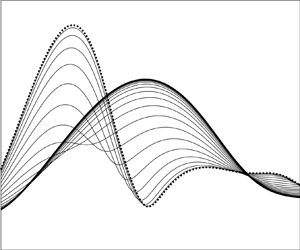
In figure 4 we show in the $\alpha$–$\omega$ plane the growth rates of instability modes with different spanwise wavenumbers for $\lambda _u(Z)$ being calculated for surface temperature distribution (2.38a,b) with (2.39). Different lines refer to different streamwise locations between $\bar {X}=-1.2$ (thick solid lines) and $\bar {X}=0$ (thick dotted lines) with an increment of $0.05$. The thick solid lines can be considered as representing the growth rates of first Mack modes. Due to the local nature of the instability problem as well as the symmetry of the wall temperature (2.37) and the wall shear (2.40), it suffices to calculate only the upstream half of the heating region. Six representative spanwise wavenumbers ($\beta _{TS}/\beta =0.2$, $0.3$, $0.4$, $0.6$, $0.7$ and $0.8$) are chosen. For weakly three-dimensional modes with $\beta _{TS}<0.5\beta$ (figures 4a–c), there is always a range of frequencies in which the growth rate $(-\alpha _i)$ of instability modes decreases monotonically from the upstream to the centre of the elements. For example, for $\beta _{TS}/\beta =0.3$, a stabilising effect occurs for $4<\omega <6$. For sufficiently low and high frequencies, the growth rate increases monotonically. Between the low and intermediate frequencies, the growth rate varies non-monotonically. However, for strongly three-dimensional modes with $\beta _{TS}>0.5\beta$, figures 4(d–f) show that the growth rate $(-\alpha _i)$ increases monotonically with $\bar {X}$ for almost all frequencies with the exception for high values in figure 4(f), and the heating elements play a broad destabilising role. Non-continuous variations of the growth rate $(-\alpha _i)$ with the frequency $\omega$ can be observed for high frequencies in figures 4(a,f). Such discontinuities will be discussed later.

Figure 4.

Growth rates vs the frequency $\omega$ at various streamwise locations $\bar {X}$ for $S(Z)=\cos (2{\rm \pi} Z)$. Thick solid lines: $\bar {X}=-1.2$; thick dotted lines: $\bar {X}=0$. Different lines in between refer to different streamwise locations with an increment of $0.05$. The red dotted lines represent the continuation of the mode to the right/left by increasing/descreasing $\omega$ for fixed $\bar {X}=0$.

As in Kátai & Wu (Reference Kátai and Wu2020), for $\beta _{TS}/\beta =0.5$ (i.e. $q=0.5$), we have also identified antisymmetric and symmetric modes, whose eigenfunctions $\hat {p}_3(Z)$ are odd and even functions of $Z$, respectively, and their growth rates are shown in figure 5(a,b). The instability characteristics of these antisymmetric/symmetric modes are similar to that of weakly/strongly three-dimensional modes in figure 4, and can be regarded as the continuation of the latter, respectively. The spanwise distributions of the lower-deck pressure $\hat {p}_3(Z)$ of these modes, which are also referred to as subharmonic modes, are displayed in figure 6(a,b). In addition to $q=1/2$, antisymmetric/symmetric modes are also found for $q=k/2$ with $k=2,3,\ldots$. Of these, $q=1$ ($k=2$) represents fundamental parametric resonance. Different from the subharmonic ones, figure 5(c,d) shows nearly the same variation (increase) of the growth rates for antisymmetric and symmetric fundamental modes. The corresponding spanwise distributions of the pressure $\hat {p}_3(Z)$ are presented in figure 6(c,d).

Figure 5.

Growth rates vs the frequency $\omega$ of subharmonic (a,b) and fundamental modes (c,d): (a,c) antisymmetric modes; (b,d) symmetric modes. Thick solid lines: $\bar {X}=-1.2$; thick dotted lines: $\bar {X}=0$. Different lines in between refer to different streamwise locations with an increment of $0.05$.

Figure 6.

Spanwise shapes $\hat {p}_3(Z)$ of symmetric (b,d) and antisymmetric (a,c) modes at $\bar {X}=0$ with $\omega =3$: (a,b) subharmonic modes; (c,d) fundamental modes.

Calculations are carried out also for heating elements with larger spanwise spacing, corresponding to $\beta ={\rm \pi}$. The growth rates are displayed in figure 7. Compared with the case of $\beta =2{\rm \pi}$ shown in figure 4, the instability characteristics are broadly similar, but appreciable differences arise. For example, for $\beta _{TS}=0.4\beta$ (figure 7b), a distinctive band of high-frequency Mack modes are destabilised to become as dominant as destabilised low-frequency modes, and this band is marked by non-continuous variations with the frequency. For $\beta _{TS}>0.5\beta$, the modes within a small range of frequencies are stabilised by an amount that becomes rather moderate as $\beta _{TS}$ increases.

Figure 7.

Growth rates vs the frequency $\omega$ at various streamwise locations $\bar {X}$ for $S(Z)=\cos ({\rm \pi} Z)$. Thick solid lines: $\bar {X}=-1.2$; thick dotted lines: $\bar {X}=0$. Different lines in between refer to different streamwise locations with an increment of $0.05$. The red dotted lines represent the continuation of the mode to the right/left by increasing/descreasing $\omega$ for fixed $\bar {X}=0$.

A discussion of the discontinuities in figures 4 and 7 is in order. The discontinuities reflect coexistence of a multi-family of modes and ‘mode crossing’ phenomenon. The eigenvalue $\alpha (\omega,\bar {X})$ is a function of $\omega$ and $\bar {X}$. It can be calculated by using either of the two approaches: the first fixes $\bar {X}$ but varies $\omega$ gradually, and while the second fixes $\omega$ but increases $\bar {X}$ in small increments. The data in the figures were calculated by the latter approach. Each eigen mode so obtained evolves from an upstream first mode with a spanwise wavenumber $\beta _{TS}=(k+q)\beta$ with $0\leq q \leq 1/2$, and, hence, each mode can be distinguished by $(k,q)$, and be designated by $\alpha _{k,q}(\omega,\bar {X})$ with $k=0,\pm 1,\ldots$, as shown by Kátai & Wu (Reference Kátai and Wu2020). At each $\bar {X}$, these modes coexist and are intricately interlinked as $\bar {X}$ and $\omega$ vary. If $k$ and $q$ are fixed also, $\alpha _{k,q}(\omega,\bar {X})$ may not be a continuous function of $\omega$. Taking $\bar {X}=0$ as an example, a jump occurs at $\omega _c \approx 6.5$ as is shown figure 4(a), and the modes on both sides may be designated as $\alpha _{0,0.2}(\omega,\bar {X})$, which evolves from a first mode upstream with $\beta _{TS}=0.2\beta$. On the other hand, with $\bar {X}=0$ being fixed, the mode to the left of the jump with $\omega <\omega _c$ may be continued parametrically to the right by gradually increasing $\omega$, and similarly, the mode to the right of the jump with $\omega >\omega _c$ may be continued to the left by decreasing $\omega$. The results are indicated by the red dotted lines. Interestingly, these extended lines turned out to coincide with the dotted lines in figure 4(f), and the jumps in figure 4(a,f) overlap. As each mode on the dotted lines in figure 4(f) develops from an upstream first mode with $\beta _{TS}=(-1+0.2)\beta$, it is designated as $\alpha _{-1,0.2}(\omega,\bar {X})$ and so is the mode on the red extended lines in figure 4(a). Indeed, starting with a mode on this line, we can trace it back to an upstream first mode with $\beta _{TS}/\beta =0.8$. It follows that as $\omega$ crosses $\omega _c$, there is a crossover from $\alpha _{0,0.2}(\omega,\bar {X})$ to $\alpha _{-1,0.2}(\omega,\bar {X})$ despite the fact they are on the same smooth line.

The jumps in figure 7(c,d) are associated with similar crossovers of modes. Again take $\bar {X}=0$ for illustration. The discontinuous dotted curve represents the mode $\alpha _{0,0.4}(\omega,\bar {X})$. The small segment between the two jumps on the left can be continued to the smaller and larger $\omega$, whilst the dotted line to the left of the first jump is continued to the right (to connect with $\alpha _{0,0.4}(\omega,\bar {X})$). The extended lines turn out to be the same as the three segments of the dotted line in figure 7(d), and, thus, represent the mode $\alpha _{-1,0.4}(\omega,\bar {X})$, which evolves from an upstream first mode with $\beta _{TS}=(-1+0.4)\beta$. Similarly, the dotted lines to the right/left of the third jump in figure 7(c) can also be continued to the left/right, respectively. The resulting extended lines represent the mode $\alpha _{1,0.4}(\omega,\bar {X})$, which develops from an upstream first mode with $\beta _{TS}=(1+0.4)\beta$ (not shown).

Figure 8 displays the results for the heating elements with spanwise distribution $S(Z)$ given in (2.38a,b) with $s_0=0.5$, $s_1=1$ and $s_n=0$ for all $n\leq 2$, that is,

(4.6)\begin{equation} S(Z)=0.5+\cos(2{\rm \pi} Z),\end{equation}

which combines a spanwise uniform part with a simple spanwise-harmonic Fourier component. Stabilising effects can be observed for most cases except low-frequency modes for $\beta _{TS}/\beta <0.5$ plus a band of high-frequency modes for $\beta _{TS}/\beta =0.2$. Comparing figure 8 with figure 4, one notes that the addition of the spanwise uniform component leads to an opposite effect for the modes with $\beta _{TS}/\beta >0.5$, whose growth rates are substantially reduced, while for modes $\beta _{TS}/\beta <0.5$, the effect remains similar but quantitatively the combined spanwise uniform and periodic heating causes a stronger stabilising effect. These results indicate the possibility of inhibiting/enhancing first Mack modes via a suitable combination of Fourier components in the spanwise distribution $S(Z)$.

Figure 8.

Growth rates vs the frequency $\omega$ at various streamwise locations $\bar {X}$ for $S(Z)=0.5+\cos (2{\rm \pi} Z)$. Thick solid lines: $\bar {X}=-1.2$; thick dotted lines: $\bar {X}=0$. Different lines in between refer to different streamwise locations with an increment of $0.05$.

4.3. Distribution of eigenfunctions

The eigenfunction distributions in the upper and lower decks are of interest as they project distinctive features of the instability modes. Figure 9(a) displays the distribution of the upper-deck pressure at $\bar {X}=0$ of a radiating mode with $\omega =3$ and $\beta _{TS}/\beta =1$ for the spanwise distribution $S(Z)=\cos (2{\rm \pi} Z)$. Only the real part, $(\hat {p}_1(y_1,Z))_r$, is shown since the distribution of the imaginary part looks similar. As is illustrated, the mode radiates an acoustic wave to the far field while undergoing slow attenuation, which is controlled by $\alpha _i$. The profiles of several low-order Fourier components $(\bar {p}_n(y_1))_r$ are shown in figure 9(b), where $n=-1$ represents the radiating component while other components rapidly attenuate exponentially in the region $y_1=O(1)$ as shown in figure 9(c,d). That the $n=-1$ component emits a sound wave is indicated by (3.28b). For an integer $\beta _{TS}/\beta$, there is at least one value $n=-q$ ensuring $\varLambda _r<0$, and so the $n=-1$ component is radiating for modes with $\beta _{TS}/\beta =1$ (i.e. $q=1$ and $K=0$). It is worth noting that the growth rate of the mode shown is rather significant. For modes with reduced growth rates, the radiating character becomes even more prominent (see figure 12). These modes are fundamentally different from the radiating modes identified in high enthalpy boundary layers over a cooled wall (Mack Reference Mack1984; Chuvakhov & Fedorov Reference Chuvakhov and Fedorov2016).

Figure 9.

Distributions of $(\hat {p}_1)_r$ and corresponding Fourier components $(\bar {p}_n)_r$ at $\bar {X}=0$ for a radiating mode with $\omega =3$ and $\beta _{TS}/\beta =1$: (a,c) contours of $(\hat {p}_1)_r$; (b,d) profiles of $(\bar {p}_n)_r$ for several values of $n$.

Figure 10 displays the contours of the temperature and velocity disturbances in the $y_3$–$Z$ plane at three streamwise locations, $\bar {X}=-1$, $-0.5$ and $0$, for a mode with $\omega =4$ and $\beta _{TS}/\beta =0.3$; again, only the real parts, $(\hat {T}_3(y_3,Z))_r$ and $(\hat {u}_3(y_3,Z))_r$, are shown as representatives. One notes that $(\hat {T}_3)_r$ (left column) and $(\hat {u}_3)_r$ (right column) feature double- and single-deck structures, respectively. From the upstream to the centre of the elements, $(\hat {T}_3)_r$ and $(\hat {u}_3)_r$ exhibit qualitatively similar characters, but they both become progressively more concentrated in the spanwise direction with their maxima and minima moving closer to the centreline. This mode exhibits no symmetry about $Z=0$. Contours of the eigenfunction of a symmetric radiating mode with $\omega =3$ and $\beta _{TS}/\beta =1$ are shown in figure 11. A comparison with figure 10 reveals a number of differences between the eigenfunction contours of symmetric and asymmetric modes. The temperature contours of the present symmetric mode again feature two decks of cells, but the cells in each deck remain of the same sign, in contrast to the alternating signs of $(\hat {T}_3)_r$ for an asymmetric mode. Within one spanwise wavelength, contours of $(\hat {u}_3)_r$ consist of three cells with the central cell being flanked symmetrically by two side ones.

Figure 10.

Contours of $(\hat {T}_3)_r$ (a,c,e) and $(\hat {u}_3)_r$ (b,d,f) for $\omega =4$ and $\beta _{TS}/\beta =0.3$ at three locations $\bar {X}=-1$ (a,b), $-0.5$ (c,d) and $0$ (e,f). Solid and dashed lines represent contours of positive and negative values.

Figure 11.

Contours of $(\hat {T}_3)_r$ (a,c,e) and $(\hat {u}_3)_r$ (b,d,f) for a symmetric mode with $\omega =3$ and $\beta _{TS}/\beta =1$ at three locations $\bar {X}=-1$ (a,b), $-0.5$ (c,d) and $0$ (e,f). Solid and dashed lines represent contours of positive and negative values.

Figures 12 and 13 display the eigenfunction distributions respectively in the upper and lower decks of the mode with $\omega =3$ and $\beta _{TS}/\beta =1$ for the spanwise heating distribution (4.6); the parameters are otherwise the same as those in figures 9 and 11. Figure 12 indicates a more prominent acoustic radiation than that shown in figure 9. As explained earlier, this is due to the fact that the growth rate is reduced by the stabilising effect of heating in this case. Contours of the real parts of disturbance temperature and velocity, $(\hat {T}_3(y_3,Z))_r$ and $(\hat {u}_3(y_3,Z))_r$, are broadly similar to those in figure 11.

Figure 12.

Distributions of $(\hat {p}_1)_r$ and corresponding Fourier components $(\bar {p}_n)_r$ at $\bar {X}=0$ for a radiating mode with $\omega =3$ and $\beta _{TS}/\beta =1$ when heating is of form (4.6): (a,c) contours of $(\hat {p}_1)_r$; (b,d) profiles of $(\bar {p}_n)_r$ for several values of $n$.

Figure 13.

Contours of $(\hat {T}_3)_r$ (a,c,e) and $(\hat {u}_3)_r$ (b,d,f) for $\omega =3$ and $\beta _{TS}/\beta =1$ at three locations $\bar {X}=-1$ (a,b), $-0.5$ (c,d) and $0$ (e,f) when heating is of form (4.6). Solid and dashed lines represent contours of positive and negative values.