1 Introduction
Following Prandtl’s (Reference Prandtl1904) seminal work on the flow at very low viscosity, Batchelor (Reference Batchelor1956) set out to model separated eddies in the limit of infinite Reynolds number through the study of the steady laminar flow within closed streamlines. Burggraf (Reference Burggraf1966) extended the analysis to unfold the viscous structure of separated eddies at finite Reynolds number by solving the recirculating flow within a fixed finite cavity, inspired by the work of Kawaguti (Reference Kawaguti1961) in this same geometry. To overcome the computational limitation – in terms of maximum achievable Reynolds number – of numerical methods at the time, Pan & Acrivos (Reference Pan and Acrivos1967) opted for an experimental approach to try to elucidate the nature of eddies in the limiting case of infinite Reynolds number for both finite and effectively infinite aspect ratio rectangular cavities. This same set-up was also used for probing Moffatt’s (Reference Moffatt1964) predictions on corner eddies in the limiting case of creeping flow.
The incompressible shear-driven flow inside a wall-bounded cavity has since become a classical problem in fluid mechanics (Shankar & Deshpande Reference Shankar and Deshpande2000; Kuhlmann & Romanò Reference Kuhlmann, Romanò and Gelfgat2019). Its geometrical simplicity yet rich flow phenomenology make it a perfect set-up for studying a wealth of complex phenomena such as corner eddies, vortex dynamics, flow instabilities (centrifugal and shear) and turbulent transition.
The particular case of the two-dimensional flow in a square enclosure driven by the tangential motion of one of its sides, henceforth referred to as lid-driven square cavity (LDSC) flow, has become a model problem against which all sorts of numerical codes, based on a variety of alternative formulations of the incompressible Navier–Stokes equations, are frequently benchmarked. To name but a few, these include primitive variables
 $\boldsymbol{u}$
–
 $p$
(Vanka Reference Vanka1986; Bruneau & Saad Reference Bruneau and Saad2006), pure streamfunction
 $\unicode[STIX]{x1D713}$
(Ghia, Ghia & Shin Reference Ghia, Ghia and Shin1982), mixed streamfunction–vorticity
 $\unicode[STIX]{x1D713}$
–
 $\unicode[STIX]{x1D714}$
(Schreiber & Keller Reference Schreiber and Keller1983) and streamfunction–velocity
 $\unicode[STIX]{x1D713}$
–
 $\boldsymbol{u}$
(Gupta & Kalita Reference Gupta and Kalita2005) finite difference schemes;
 $\boldsymbol{u}$
–
 $p$
(Marchi, Suero & Araki Reference Marchi, Suero and Araki2009) and pure velocity
 $\boldsymbol{u}$
(Sahin & Owens Reference Sahin and Owens2003a
) finite volume discretisations;
 $\boldsymbol{u}$
–
 $p$
finite elements (Gresho & Chan Reference Gresho and Chan1990);
 $\boldsymbol{u}$
–
 $p$
(Botella & Peyret Reference Botella and Peyret1998) and
 $\unicode[STIX]{x1D713}$
–
 $\unicode[STIX]{x1D714}$
(Auteri, Quartapelle & Vigevano Reference Auteri, Quartapelle and Vigevano2002b
) spectral methods;
 $\boldsymbol{u}$
–
 $p$
discrete Galerkin finite/spectral elements (Romanò & Kuhlmann Reference Romanò and Kuhlmann2017); primitive variable incompressible smoothed particle hydrodynamics (Khorasanizade & Sousa Reference Khorasanizade and Sousa2014); and lattice Boltzmann models (Hou et al.
Reference Hou, Zou, Chen, Doolen and Cogley1995).
Lid-driven cavity flows are singular at the corners where the moving lid meets the stationary adjacent walls. This is particularly problematic for high-order discretisations, notably for spectral methods due to the global support of the expansion basis functions. A standard fourth-order polynomic regularisation has occasionally been applied to the lid velocity profile to remove the singularity (Shen Reference Shen1991; Botella Reference Botella1997). The resulting regularised cavity flow problem allegedly preserves the same qualitative dynamics as the original singular cavity, albeit at the cost of non-negligible quantitative effects. Higher-order regularisation can be enforced to preserve a constant velocity over a wide portion of the lid and still avoid the singularities at the corners (Batoul, Khallouf & Labrosse Reference Batoul, Khallouf and Labrosse1994) as a rather straightforward solution to simulate quasi-singular cavity flows. A more subtle (and sound) approach consists of explicitly subtracting the leading asymptotic expansion terms of the singularity (Botella & Peyret Reference Botella and Peyret2001; Auteri et al. Reference Auteri, Quartapelle and Vigevano2002b ), whose expressions can be found analytically (Gupta, Manohar & Noble Reference Gupta, Manohar and Noble1981). Alternatively, small leaks can be introduced at the corner junctions to overcome the singularity in the same way this might be resolved in physically realisable experimental set-ups (Sahin & Owens Reference Sahin and Owens2003a ). Given that, by their nature, low-order discretisation methods confine the effects of the singularity to a close neighbourhood of the corners with little to no impact on the bulk of the fluid domain, the most usual course of action is to simply ignore the issue altogether.
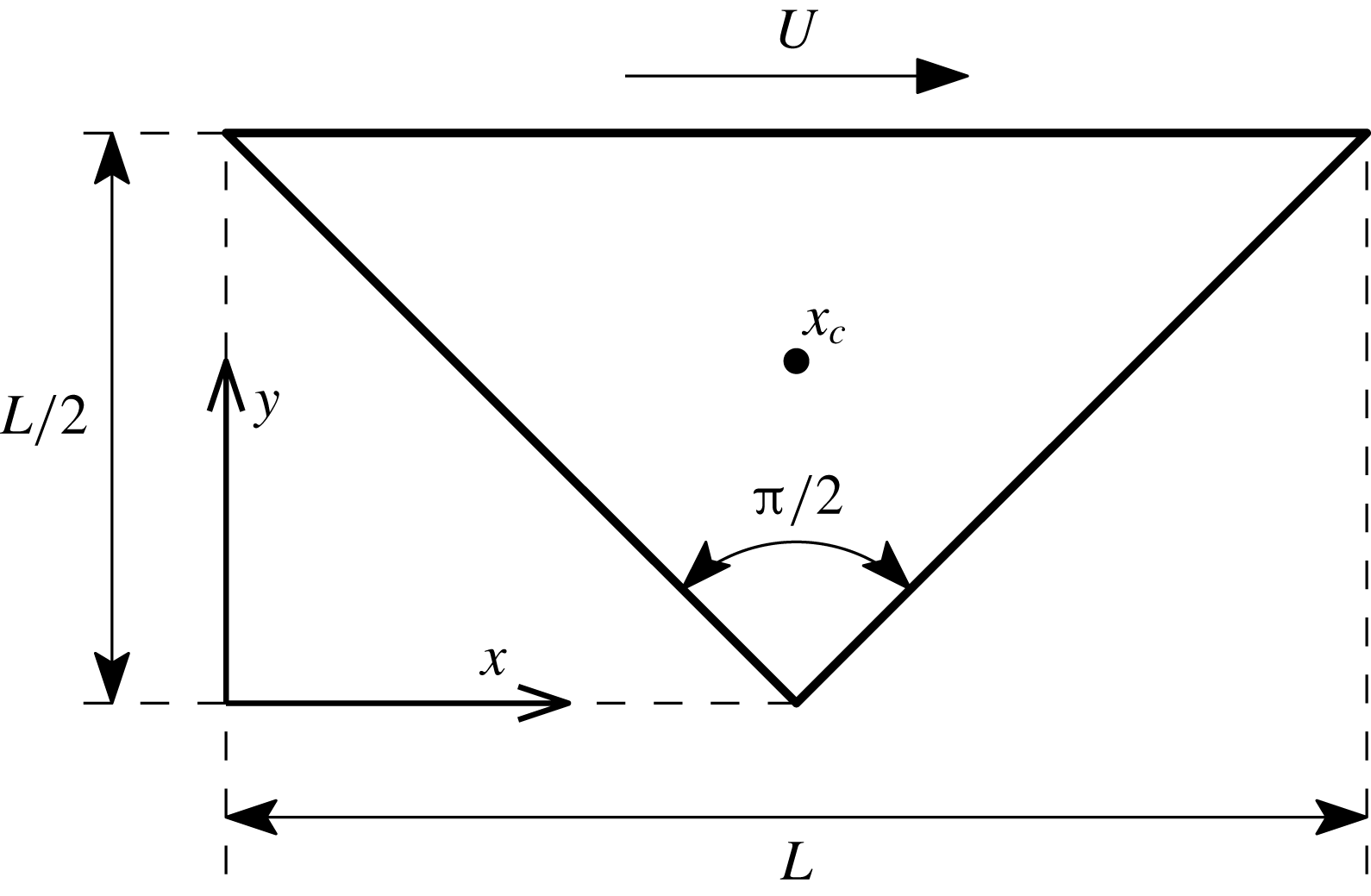
Our objective here is to unfold the transition process from the laminar base state to chaotic motion of the two-dimensional flow within a right-angled triangular cavity driven by the constant-speed tangential motion of its hypotenuse, i.e. the wall opposite the right angle (figure 1).
The two-dimensional lid-driven right-angled isosceles triangular cavity.

The destabilisation of the flow in two-dimensional cavities is relevant to the understanding of the onset of two-dimensional turbulence (Molenaar, Clercx & van Heijst Reference Molenaar, Clercx and van Heijst2005), an active research field on account of its sharing key features with the large-scale motions observed in geophysical flows (Boffetta & Ecke Reference Boffetta and Ecke2012). Wall-bounded two-dimensional vortices do indeed occur in near-shore zones, such as at the head of rip currents (Smith & Largier Reference Smith and Largier1995) or in tidal channels (Wells & van Heijst Reference Wells and van Heijst2003).
As we shall see, the onset of chaotic motion has been treated to some extent for the case of LDSC flow, while very little is known of the complete unfolding for cavities of other shapes, except that the transition process appears to follow different paths. The motivation behind our choice of a triangular geometry stems from the way in which the vortex arrangement becomes increasingly intricate with Reynolds number escalation, even before the flow becomes non-stationary. In particular, the triangular set-up we have adopted acts as a model for the onset of chaos, a necessary step towards two-dimensional turbulence, when the base flow consists of a strong jet that impinges on a no-slip wall in a narrowly confined domain.
A thorough dissection of what has been done on square cavities, as well as other geometries bearing some resemblance to our hypotenuse-driven right-angled isosceles triangular cavity (or simply lid-driven triangular cavity, LDTC) flow, is in order. For a detailed comprehensive analysis of lid-driven cavity flows, we refer the reader to the dedicated review by Shankar & Deshpande (Reference Shankar and Deshpande2000), and references therein. Exhaustive up-to-date results can be found in Kuhlmann & Romanò (Reference Kuhlmann, Romanò and Gelfgat2019).
The first instability of the two-dimensional LDSC flow is of three-dimensional nature. This was first realised by Koseff & Street (Reference Koseff and Street1984) experimentally in a cavity of span-to-width aspect ratio
 $\unicode[STIX]{x1D6EC}=3$
. Certain aspects of the three-dimensionalisation of the flow could be ascribed to end-wall effects, but the appearance of Taylor–Görtler-like vortices pointed to a legitimate three-dimensional instability of the underlying two-dimensional flow. These vortices originate from a centrifugal instability caused by the concavity of the spanwise core vortex streamlines in the presence of the bottom downstream corner vortex. Further experiments by Aidun, Triantafillopoulos & Benson (Reference Aidun, Triantafillopoulos and Benson1991) and Benson & Aidun (Reference Benson and Aidun1992) on a cavity with the same proportions (and a small throughflow that allegedly had little effect) placed the instability at
 $Re_{H}\simeq 875\pm 50$
, which gave rise to a periodic three-dimensional state in the form of spiral waves of non-dimensional angular frequency
 $\unicode[STIX]{x1D714}_{H}\simeq 0.7$
. They also identified a transition to chaotic motion at
 $Re<1000$
via a Ruelle–Takens-type path (Ruelle & Takens Reference Ruelle and Takens1971; Newhouse, Ruelle & Takens Reference Newhouse, Ruelle and Takens1978), as suggested by the detection of an intervening quasi-periodic state. Numerical stability analysis later showed that the infinite span system undergoes a Hopf bifurcation at
 $Re_{H}\simeq 920$
with spanwise wavenumber
 $\unicode[STIX]{x1D705}_{H}\simeq 7.4$
and
 $\unicode[STIX]{x1D714}_{H}\simeq 0.495$
(Ding & Kawahara Reference Ding and Kawahara1999). Albensoeder, Kuhlmann & Rath (Reference Albensoeder, Kuhlmann and Rath2001) showed numerically that the first instability is in fact steady (a pitchfork-type disruption of the translational invariance implied by the
 $O(2)=SO(2)\rtimes Z_{2}$
spanwise symmetry of the problem; here,
 $O(2)$
is the orthogonal group in two dimensions, which results from the semidirect product of
 $SO(2)$
, the special orthogonal or rotation group in two dimensions – spanwise translational invariance – and the normal subgroup
 $Z_{2}$
, the second-order cyclic or dihedral group – reflection with respect to planes orthogonal to the spanwise direction) and occurs for
 $Re_{P}\simeq 785$
and
 $\unicode[STIX]{x1D705}_{P}\simeq 15.4$
. The resulting three-dimensional flow consists of an infinite array of steady Taylor–Görtler vortices. The stability analysis was supplemented with experimental results for a cavity with
 $\unicode[STIX]{x1D6EC}=6.55$
that confirmed the appearance of Taylor–Görtler vortices in the centre of the domain, away from the side walls. They also detected a secondary transition at around
 $Re_{H}\simeq 930\sim 980$
, consisting of the intermittent ejection of spiralling waves from the central pattern towards either side. Theofilis, Duck & Owen (Reference Theofilis, Duck and Owen2004) and Non, Pierre & Gervais (Reference Non, Pierre and Gervais2006) confirmed through linear stability analysis the occurrence of the first steady bifurcation and reported additional bifurcations of the base flow that broke the translational invariance and the reflection symmetry simultaneously, among which the one at
 $Re\simeq 922$
with
 $\unicode[STIX]{x1D705}\simeq 15.8$
and
 $\unicode[STIX]{x1D714}_{H}\simeq 0.496$
seemed to be related to the secondary transition observed by Albensoeder et al. (Reference Albensoeder, Kuhlmann and Rath2001). This type of bifurcation gives rise to branches of conjugate-symmetric spanwise-travelling waves much as observed in the aforementioned experiments. The frequency associated with this kind of solutions is degenerate in the sense that it represents a mere drift along the group orbit such that the resulting drift dynamics is in fact trivial (Krupa Reference Krupa1990). The situation is somewhat different in experiments, where the presence of end walls destroys the translational invariance of the system and the appearance of Eckman layers results in a degeneration of the infinite system dynamics, such that nominally two-dimensional flow is confined to only the central region of the cavity at sufficiently low Reynolds numbers, the appearance of only a finite number of Taylor–Görtler vortices follows the first bifurcation and the secondary Hopf bifurcation of the resulting fully three-dimensional flow state induces real temporal dynamics. The onset of time dependence becomes yet more involved when the bounding end walls are close to one another and the span-to-depth/length cavity ratio is not sufficiently large. This is the case of the cubic lid-driven cavity flow (Lopez et al.
Reference Lopez, Welfert, Wu and Yalim2017), for which the subcritical nature of the first instability of the base steady flow and its interplay with a second bifurcation set the stage for intermittent bursts at irregular times.
In spite of the known early three-dimensionalisation of the base two-dimensional LDSC flow, many efforts have been devoted to elucidating its linear stability to purely two-dimensional perturbations. This has extended the value of the lid-driven cavity flow as a benchmark problem beyond the realm of nonlinear time-steppers and steady-state solvers to the wider domain of stability analysis and bifurcation-tracking methods. But the relevance of analysing bifurcation sequences of unstable solutions reaches much further than its mere use for code validation. The strange saddle that is embedded in chaotic motion, and therefore organises turbulent dynamics, consists of collections of unstable solutions and their connecting manifolds (Procaccia Reference Procaccia1988). Restricting the analysis to certain symmetries or severely truncated domains, however unrealistic this may appear from a merely experimental point of view, allows for a detailed analysis that is otherwise unaffordable and provides access to the basic ingredients that might be at play in the real problem (Hof et al.
Reference Hof, van Doorne, Westerweel, Nieuwstadt, Faisst, Eckhardt, Wedin, Kerswell and Waleffe2004; de Lozar et al.
Reference de Lozar, Mellibovsky, Avila and Hof2012). In the case of systems that feature translational invariance along an extended spatial coordinate, one such possible symmetry restriction consists of constraining the dynamics to be two-dimensional (Jimenez Reference Jimenez1990; Mellibovsky & Meseguer Reference Mellibovsky and Meseguer2015). The first two-dimensional instability of LDSC flow is a supercritical Hopf bifurcation. Its exact occurrence in parameter space has been subject to much controversy, as it is extremely dependent on both resolution and the way the corner singularity is treated. Shen (Reference Shen1991) provided the first estimate for regularised LDSC flow from mere nonlinear time evolution, in combination with
 $Re$
bisection to find the border between steady and periodic dynamics. His estimate was later refined by Fortin et al. (Reference Fortin, Jardak, Gervais and Pierre1997) and Abouhamza & Pierre (Reference Abouhamza and Pierre2003), through Newton steady-state computation and Arnoldi stability analysis, to the now widely accepted critical point at
 $Re_{H}\simeq 10\,267\pm 12$
and non-dimensional angular frequency
 $\unicode[STIX]{x1D714}_{H}\simeq 2.080$
.
The first singular LDSC flow stability analysis was due to Poliashenko & Aidun (Reference Poliashenko and Aidun1995). Steady-state tracking with a Newton solver and direct stability analysis provided a fair estimate for the Hopf point, while extrapolation to zero of a square-root fit to the oscillation amplitude of bifurcated periodic orbits obtained through nonlinear time evolution unveiled its supercritical nature. Numerous computational studies have since aimed at providing the exact location of this first instability. Some researchers have followed Poliashenko & Aidun (Reference Poliashenko and Aidun1995) in employing direct or Arnoldi linear stability analysis on steady states tracked by continuation methods or obtained from nonlinear time evolution (Fortin et al.
Reference Fortin, Jardak, Gervais and Pierre1997; Tiesinga, Wubs & Veldman Reference Tiesinga, Wubs and Veldman2002; Abouhamza & Pierre Reference Abouhamza and Pierre2003; Sahin & Owens Reference Sahin and Owens2003b
; Boppana & Gajjar Reference Boppana and Gajjar2010; Kalita & Gogoi Reference Kalita and Gogoi2016; Nuriev, Egorov & Zaitseva Reference Nuriev, Egorov and Zaitseva2016), while others have aimed at analysing the decay rate of linear perturbations onto the stable steady-state branch as the bifurcation is approached (Bruneau & Saad Reference Bruneau and Saad2006; Boppana & Gajjar Reference Boppana and Gajjar2010). Linear stability analysis of low-dimensional projections on a reduced number of proper orthogonal decomposition modes has also provided fair estimates (Cazemier, Verstappen & Veldman Reference Cazemier, Verstappen and Veldman1998). Direct numerical simulation has also been used to determine the Hopf point by adjusting a square-root fit to the Reynolds number dependence of the amplitude of the periodic orbits branch issued from the bifurcation (Cazemier et al.
Reference Cazemier, Verstappen and Veldman1998; Peng, Shiau & Hwang Reference Peng, Shiau and Hwang2003; Murdock, Ickes & Yang Reference Murdock, Ickes and Yang2017). This approach has occasionally been used as a mere complement to steady-state computation and stability analysis to provide evidence of the supercritical nature of the bifurcation (Fortin et al.
Reference Fortin, Jardak, Gervais and Pierre1997). Finally, straightforward nonlinear time evolution, combined with Reynolds bisection to find the border separating convergence onto steady states from departure towards limit cycles, has also allowed estimation of the critical point (Auteri, Parolini & Quartapelle Reference Auteri, Parolini and Quartapelle2002a
; Lin, Chang & Lin Reference Lin, Chang and Lin2013; Zhuo, Zhong & Cao Reference Zhuo, Zhong and Cao2013). All in all, there is now wide consensus that the Hopf bifurcation of the singular lid-driven cavity flow is supercritical and occurs at
 $Re_{H}\sim 8020$
with angular frequency
 $\unicode[STIX]{x1D714}_{H}\sim 2.83$
.
Most of the aforementioned studies involving nonlinear time evolution have gone beyond the first bifurcation to show the onset of quasi-periodic motion (including frequency locking episodes) and the eventual transition to chaos (Poliashenko & Aidun Reference Poliashenko and Aidun1995; Cazemier et al.
Reference Cazemier, Verstappen and Veldman1998; Auteri et al.
Reference Auteri, Parolini and Quartapelle2002a
). Auteri et al. (Reference Auteri, Parolini and Quartapelle2002a
) report quasi-periodic states with a modulational angular frequency of around
 $\unicode[STIX]{x1D714}_{NS}\simeq 1.72$
on top of the oscillation frequency (rotation number
 $r=\unicode[STIX]{x1D714}_{H}/\unicode[STIX]{x1D714}_{NS}\simeq 1.64$
), in fair agreement with the Neimark–Sacker bifurcation found by Cazemier et al. (Reference Cazemier, Verstappen and Veldman1998) with their truncated proper orthogonal decomposition model through Floquet stability analysis of the branch of periodic orbits issued from the preceding Hopf bifurcation. Additional instabilities predicted by the model such as period-doubling bifurcations seem to be an artifact of its low dimensionality. In their attempt to unfold the route to chaos, Peng et al. (Reference Peng, Shiau and Hwang2003) detected bistability (possibly associated with hysteretical behaviour), a seemingly unrelated Neimark–Sacker bifurcation and direct and inverse period-doubling cascades that have not been confirmed by any other study since. Tiesinga et al. (Reference Tiesinga, Wubs and Veldman2002) analysed the stability of the base steady flow beyond the first bifurcation and found a succession of additional supercritical Hopf bifurcations, whose associated imaginary parts could be traced back to distinct spectral frequency peaks of a chaotic direct numerical simulation at
 $Re=10\,000$
by Cazemier et al. (Reference Cazemier, Verstappen and Veldman1998). Floquet stability analysis of the periodic orbit branch issued from the original Hopf revealed a Neimark–Sacker bifurcation at
 $Re_{NS}\sim 9150$
with properties perfectly compatible with quasi-periodic solutions reported in the literature at slightly higher Reynolds numbers. The branch issued from the second Hopf (
 $Re_{H_{2}}\sim 8600$
) undergoes a stabilising Neimark–Sacker bifurcation at around
 $Re_{NS_{2}}\sim 8800$
, thus foreseeing bistability over a fairly wide range of Reynolds numbers. As an aside, the uniqueness of the laminar base state has recently been belied by Nuriev et al. (Reference Nuriev, Egorov and Zaitseva2016) who unveiled, using homotopy continuation, the existence of multiple disconnected branches of unstable steady states that appear in saddle-node bifurcations at Reynolds numbers as low as 5800.
Not many researchers have ventured into analysing the stability of LDSC flow using the lattice Boltzmann method (LBM). Lin et al. (Reference Lin, Chang and Lin2013) and Zhuo et al. (Reference Zhuo, Zhong and Cao2013) produced rather high estimates for the Hopf point using Reynolds bisection on simulations done with filter matrix LBM and multiple relaxation time (MRT) LBM, respectively. A much finer prediction has recently been obtained by Murdock et al. (Reference Murdock, Ickes and Yang2017) through the periodic oscillation amplitude square-root fit and extrapolation procedure. The improved accuracy in the prediction is possibly related to their using higher resolutions with the incompressible LBM (iLBM) model of Guo, Shi & Wang (Reference Guo, Shi and Wang2000), in conjunction with MRT as implemented by Du, Shi & Chen (Reference Du, Shi and Chen2006).
Popular as LDSC flow has become, it represents but one possibility among the infinite shapes that a shear-driven cavity may have and, as it happens, even very slight variations in the geometry entail dramatic changes in terms of flow topology and vortex dynamics. For instance, small variations in the aspect ratio rendering the cavity effectively rectangular make the first three-dimensional instability switch from steady to oscillatory (Albensoeder et al. Reference Albensoeder, Kuhlmann and Rath2001; Theofilis et al. Reference Theofilis, Duck and Owen2004). Back to the two-dimensional problem, the stability of the base flow in deep rectangular cavities (Goodrich, Gustafson & Halasi Reference Goodrich, Gustafson and Halasi1990; Abouhamza & Pierre Reference Abouhamza and Pierre2003; Boppana & Gajjar Reference Boppana and Gajjar2010; Lin et al. Reference Lin, Chang and Lin2013; Zhuo et al. Reference Zhuo, Zhong and Cao2013) has been studied in some detail. Shallow cavities have rarely been given attention (Poliashenko & Aidun Reference Poliashenko and Aidun1995) beyond the bare determination of the steady-flow vortex patterns (Gupta & Kalita Reference Gupta and Kalita2005; Cheng & Hung Reference Cheng and Hung2006).
Triangular cavities have been analysed in several configurations, and then only for steady-state flow pattern illustration at low to moderate Reynolds numbers. These include equilateral (McQuain et al. Reference McQuain, Ribbens, Wang and Watson1994; Ribbens, Watson & Wang Reference Ribbens, Watson and Wang1994; Li & Tang Reference Li and Tang1996; Gaskell, Thompson & Savage Reference Gaskell, Thompson and Savage1999; Kohno & Bathe Reference Kohno and Bathe2006; Erturk & Gokcol Reference Erturk and Gokcol2007; Paramane & Sharma Reference Paramane and Sharma2008; Pasquim & Mariani Reference Pasquim and Mariani2008), various aspect ratio isosceles (McQuain et al. Reference McQuain, Ribbens, Wang and Watson1994; Jyotsna & Vanka Reference Jyotsna and Vanka1995; Gaskell et al. Reference Gaskell, Thompson and Savage1999; Jagannathan, Mohan & Dhanak Reference Jagannathan, Mohan and Dhanak2014) and a few scalene (Li & Tang Reference Li and Tang1996) triangular geometries.
Gonzalez et al. (Reference Gonzalez, Ahmed, Kuehnen, Kuhlmann and Theofilis2011) and Ahmed & Kuhlmann (Reference Ahmed and Kuhlmann2012) have shown both experimentally and numerically that, as for LDSC flow, the first instability in lid-driven right-angled triangular cavities of various length-to-depth aspect ratios with the moving wall adjacent to the rectangular corner is also three-dimensional. For an aspect ratio such that the cavity is an isosceles triangle with the lid moving towards the rectangular corner, the leading mode is complex (oscillatory) and becomes unstable at
 $Re=777.9$
(
 $Re=730\pm 20$
according to experiments) with spanwise wavenumber
 $k_{c}=10.3$
(
 $k_{c}=11.2\pm 0.6$
) and angular frequency
 $\unicode[STIX]{x1D714}_{c}=1.14$
(
 $\unicode[STIX]{x1D714}_{c}=1.121\pm 0.05$
), values that are fully consistent with those of a rectangular cavity of aspect ratio 0.5, for which
 $(Re_{c},k_{c},\unicode[STIX]{x1D714}_{c})=(706,10.6,1.16)$
(Albensoeder et al.
Reference Albensoeder, Kuhlmann and Rath2001). When the lid moves away from the rectangular corner instead, the leading mode is real and becomes unstable somewhat earlier at
 $Re=540.2$
(
 $Re=570\pm 20$
experimentally) with spanwise wavenumber
 $k_{c}=2.86$
(
 $k_{c}=2.89\pm 0.11$
). Taking shallower aspect ratios,
 $Re_{c}$
is shifted to higher values and up to five distinct instability modes of various spanwise wavenumbers, some steady, some oscillatory, are observed (Ahmed & Kuhlmann Reference Ahmed and Kuhlmann2012). As long as the flow remains two-dimensional, at
 $Re=500$
, a propensity for boundary layer separation (in experiments), or at least flow deceleration (in numerics), is observed on the slanted wall when the top lid moves away from the sharp corner towards the rectangular corner. This same effect has been reported by Erturk & Gokcol (Reference Erturk and Gokcol2007) on the same exact configuration and also for an equilateral triangle, showing that the separated zone evolves into a vortical separation bubble as
 $Re$
is increased. As a matter of fact, this feature is discernible in all aforementioned studies of equilateral triangular cavities reaching beyond
 $Re=500$
. When the top lid moves away from the right-angled corner instead, the primary vortex becomes elongated along the top lid, with a bias towards the downstream acute corner. This effect is already perceptible at
 $Re=1000$
and becomes more pronounced as
 $Re$
is further increased. At higher
 $Re\gtrsim 3000$
, however, published results disagree as to the flow topology inside the equilateral triangular cavity. While some studies point to the further development of the vortical separation bubble on the upstream wall (Kohno & Bathe Reference Kohno and Bathe2006), others report a downstream-biased elongated-top-vortex arrangement along the moving lid (Pasquim & Mariani Reference Pasquim and Mariani2008).
Steady solutions for our particular configuration of interest (LDTC) have been computed by Erturk & Gokcol (Reference Erturk and Gokcol2007) and Gaskell et al. (Reference Gaskell, Thompson and Savage1999) in the case of Stokes flow and very low Reynolds numbers up to 100, and by Sidik & Munir (Reference Sidik and Munir2012) up to
 $Re=10\,000$
. Ozalp, Pinarbasi & Sahin (Reference Ozalp, Pinarbasi and Sahin2010) performed experiments in a water channel of open right-angled triangular cavity flow at
 $Re\in [1230{-}1700]$
, but any attempt of comparison with our numerical analysis is rendered futile by the intrinsic three-dimensionality of the flow in this Reynolds regime and by the fact that, in their rig, the fluid in the cavity was driven by an outer flow and not a rigid lid.
The best chance for comparison with our results, if only qualitatively, is offered by the MRT-iLBM lid-driven isosceles trapezoidal cavity simulations of Zhang, Shi & Chai (Reference Zhang, Shi and Chai2010). In a trapezoidal cavity with height-to-length aspect ratio
 $\unicode[STIX]{x1D6E4}=\sqrt{3}/3\simeq 0.577$
(0.5 in our case) and corner angles of
 $60^{\circ }$
(to be compared with
 $45^{\circ }$
for the right-angled isosceles triangle), they detected a non-trivial path from laminar flow to chaos that included a Hopf bifurcation between
 $Re=7500$
and
 $8150$
and, possibly, a Neimark–Sacker bifurcation between
 $8500$
and
 $10\,000$
as hinted at by a seemingly frequency-locked quasi-periodic solution at this latter Reynolds number.
The paper is structured as follows. In § 2 we present the problem formulation and the numerical approach that we adopt. The various types of solutions found are presented in § 3, alongside a detailed description and characterisation. The transitions between different states are discussed in § 4 in the light of dynamical systems and bifurcation theory. Some concluding remarks are finally summarised in § 5.
2 Problem statement and numerical approach
2.1 The lid-driven right-angled isosceles cavity flow
Consider an incompressible flow in a two-dimensional right-angled isosceles triangular cavity driven by the tangential motion of its hypotenuse at constant velocity (LDTC; figure 1). The flow dynamics is governed by the incompressible Navier–Stokes equations, which, after suitable non-dimensionalisation with lid size
 $L$
and lid velocity
 $U$
as length and velocity scales, result in
 $$\begin{eqnarray}\left.\begin{array}{@{}c@{}}\unicode[STIX]{x2202}_{t}\boldsymbol{u}+(\boldsymbol{u}\boldsymbol{\cdot }\unicode[STIX]{x1D735})\boldsymbol{u}=-\unicode[STIX]{x1D735}p+{\displaystyle \frac{1}{Re}}\unicode[STIX]{x0394}\boldsymbol{u},\\ \unicode[STIX]{x1D735}\boldsymbol{\cdot }\boldsymbol{ u}=0.\end{array}\right\}\end{eqnarray}$$
Here,
 $\boldsymbol{u}=\boldsymbol{u}(\boldsymbol{x};t)=(u,v)$
and
 $p=p(\boldsymbol{x};t)$
are the velocity and pressure fields,
 $\boldsymbol{x}=(x,y)$
and
 $t$
are the spatial and time coordinates and
 $Re=UL/\unicode[STIX]{x1D708}$
is the Reynolds number, with
 $\unicode[STIX]{x1D708}$
the kinematic viscosity of the fluid. No-slip Dirichlet boundary conditions
 $\boldsymbol{u}(\boldsymbol{x}_{\mathit{w}};t)=\mathbf{0}$
are imposed on both side walls while a constant tangential unit velocity is imposed on the top wall or lid
 $\boldsymbol{u}(\boldsymbol{x}_{\mathit{l}};t)=(1,0)$
.
Solutions will be characterised through the two velocity components at the centre of the cavity (
 $u_{c}$
,
 $v_{c}$
) and the lid shear force coefficient
 $$\begin{eqnarray}\left.\begin{array}{@{}c@{}}\left(u_{c}(t),v_{c}(t)\right)\equiv \boldsymbol{u}_{c}(t)=\boldsymbol{u}(\boldsymbol{x}_{c};t);\quad \boldsymbol{x}_{c}=(0.5,0.25),\\ C_{F}(t)\equiv \displaystyle {\displaystyle \frac{F}{{\textstyle \frac{1}{2}}\unicode[STIX]{x1D70C}LU^{2}}}={\displaystyle \frac{2}{Re}}\int _{0}^{1}\unicode[STIX]{x2202}_{y}u(\boldsymbol{x}_{l};t)\,\text{d}x;\quad \boldsymbol{x}_{l}=(x,0.5).\end{array}\right\}\end{eqnarray}$$
Wall shear diverges at either end of the lid due to corner singularities. The total shear force is therefore defined by an improper integral that we choose to approximate with an open Newton–Cotes-type quadrature. The LBM is of second-order accuracy. For consistency, we have chosen to employ second-order methods in the computation of the lid driving shear force. The wall-normal derivative of horizontal velocity has been estimated with second-order finite differences, and its integral over the lid approximated with Simpson’s rule. To avoid the singular end points, Simpson’s rule has been replaced with the midpoint rule in the immediate vicinity of the corners. We must admit that the lid force computation is not particularly accurate, but it flawlessly fulfils its purpose as a phase space variable as long as simulations are run on the same exact grid. Resolution changes have a large impact on
 $C_{F}$
, such that lid force coefficient cannot be used for mesh convergence analysis.
We have made extensive use of first-recurrence or Poincaré maps in order to characterise periodic and quasi-periodic solutions and to analyse their stability. Interpreted as an infinite-dimensional continuous-time dynamical system, the Navier–Stokes equations in the LDTC generate a flow (a trajectory) in phase space (the set of all possible system configurations, understood here as all possible velocity/pressure fields). By conveniently picking a hyperplane in phase space that is transversal to the flow (the Poincaré section), the corresponding Poincaré map is defined as the discrete-time dynamical system that maps one crossing of this hyperplane to the next. Periodic orbits and quasi-periodic solutions of the continuous-time dynamical system are thus reduced to fixed points and discrete periodic orbits, respectively, of the associated Poincaré map. We visualise LDTC solutions both in physical space via flow-field snapshots (be it streamfunction isocontours or vorticity colour maps) and in phase space, using two-dimensional projections of trajectories.
In order to produce vorticity colour maps and streamfunction contour plots, vorticity and streamfunction have been approximated with second-order central differences and second-order quadratures, respectively.
2.2 The iLBM
Here we chose to simulate the fluid flow in the cavity using the LBM (Chen & Doolen Reference Chen and Doolen1998). The discrete kinetic equation (or lattice Boltzmann equation) for the particle distribution function reads
 $$\begin{eqnarray}f_{i}(\boldsymbol{x}+\boldsymbol{e}_{i}\unicode[STIX]{x0394}x,t+\unicode[STIX]{x0394}t)-f_{i}(\boldsymbol{x},t)=-{\displaystyle \frac{1}{\unicode[STIX]{x1D70F}}}[f_{i}(\boldsymbol{x},t)-f_{i}^{eq}(\boldsymbol{x},t)],\end{eqnarray}$$
where
 $f_{i}(\boldsymbol{x},t)=f(\boldsymbol{x},\boldsymbol{e}_{i},t)$
is the discrete single-particle velocity distribution function in the momentum direction
 $\boldsymbol{e}_{i}$
, and density
 $\unicode[STIX]{x1D70C}$
and momentum
 $\unicode[STIX]{x1D70C}\boldsymbol{u}$
are defined as particle velocity moments of the distribution function:
 $$\begin{eqnarray}\left.\begin{array}{@{}c@{}}\unicode[STIX]{x1D70C}=\displaystyle \mathop{\sum }_{i}f_{i},\\ \unicode[STIX]{x1D70C}\boldsymbol{u}=\displaystyle \mathop{\sum }_{i}\boldsymbol{e}_{i}\,f_{i}.\end{array}\right\}\end{eqnarray}$$
The left-hand side of (2.3) represents the streaming step in the method, with
 $\unicode[STIX]{x0394}x$
and
 $\unicode[STIX]{x0394}t$
the lattice spacing and time step, respectively. The right-hand side corresponds to the collision step. The collision operator by Bhatnagar, Gross & Krook (Reference Bhatnagar, Gross and Krook1954) (BGK) naturally arises from assuming that
 $\unicode[STIX]{x0394}x$
and
 $\unicode[STIX]{x0394}t$
are small and of the same order
 $\unicode[STIX]{x1D700}$
, Taylor-expanding in space and time up to second order and then employing a formal multiscaling Chapman–Enskog expansion on the resulting continuum equation, allowing for different time scales for advection and diffusion and assuming that the local particle distribution relaxes to an equilibrium state at a single rate. Function
 $f_{i}^{eq}$
is the equilibrium distribution function and
 $\unicode[STIX]{x1D70F}$
is the non-dimensional collision relaxation time.
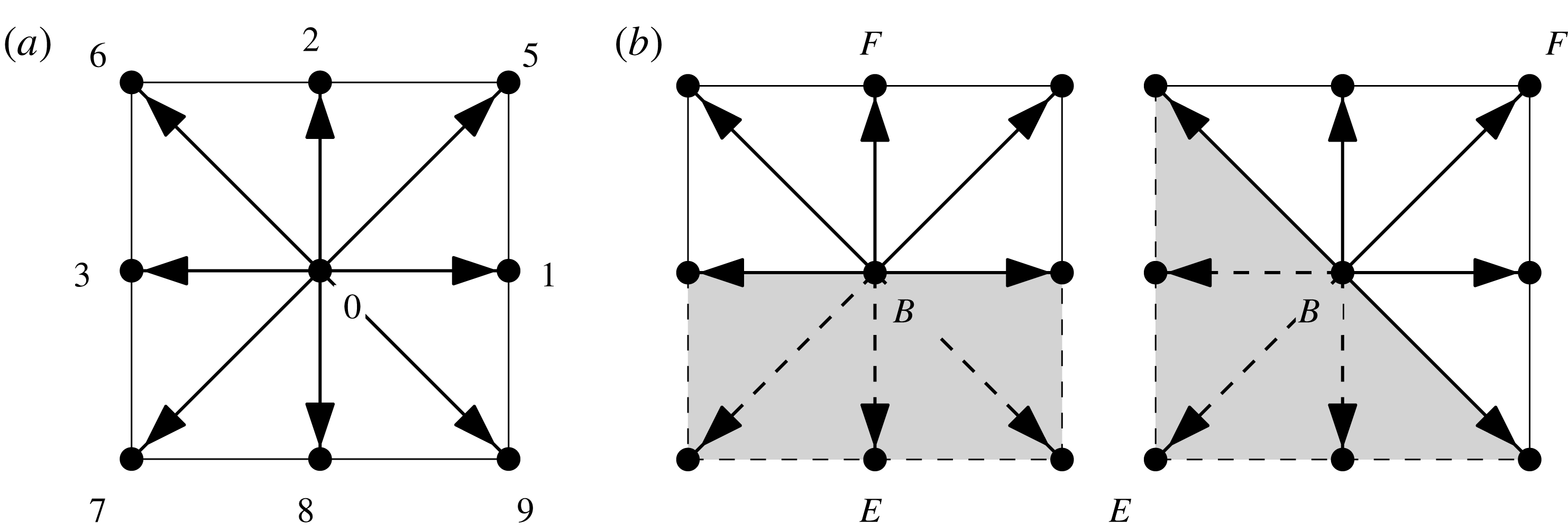
The D2Q9 lattice Boltzmann model. (a) Discrete momentum directions. (b) Treatment of flat and diagonal wall boundary conditions.

We adopt the nine-bit D2Q9 lattice Boltzmann model of Qian, D’Humières & Lallemand (Reference Qian, D’Humières and Lallemand1992), corresponding to a two-dimensional problem on a square lattice with nine discrete momentum directions as shown in figure 2(a). The discrete momentum directions are given by
 $$\begin{eqnarray}\boldsymbol{e}_{i}=\left\{\begin{array}{@{}ll@{}}(0,0) & i=0\\ (\cos \left((i-1)\unicode[STIX]{x03C0}/2\right),\sin \left((i-1)\unicode[STIX]{x03C0}/2\right)) & i\in \{1,2,3,4\}\\ (\cos \left((2i-9)\unicode[STIX]{x03C0}/4\right),\sin \left((2i-9)\unicode[STIX]{x03C0}/4\right))\sqrt{2} & i\in \{5,6,7,8\}.\end{array}\right.\end{eqnarray}$$
Using the classic equilibrium distribution function
 $$\begin{eqnarray}f_{i}^{\mathit{eq}}=\unicode[STIX]{x1D70C}\left[w_{i}+s_{i}(\boldsymbol{u}(\boldsymbol{x};t))\right],\end{eqnarray}$$
with
 $$\begin{eqnarray}s_{i}(\boldsymbol{u})=w_{i}\left[3{\displaystyle \frac{\boldsymbol{e}_{i}\boldsymbol{\cdot }\boldsymbol{u}}{c}}+{\displaystyle \frac{9}{2}}{\displaystyle \frac{(\boldsymbol{e}_{i}\boldsymbol{\cdot }\boldsymbol{u})^{2}}{c^{2}}}-{\displaystyle \frac{3}{2}}{\displaystyle \frac{\Vert \boldsymbol{u}\Vert ^{2}}{c^{2}}}\right],\end{eqnarray}$$
and weights
 $$\begin{eqnarray}w_{i}=\left\{\begin{array}{@{}ll@{}}4/9 & i=0\\ 1/9 & i\in \{1,2,3,4\}\\ 1/36 & i\in \{5,6,7,8\},\end{array}\right.\end{eqnarray}$$
where
 $c=\unicode[STIX]{x0394}x/\unicode[STIX]{x0394}t$
is the particle velocity across the lattice, the compressible Navier–Stokes equations are recovered in the limit of vanishing Mach number. The pressure is
 $p=c_{s}^{2}\unicode[STIX]{x1D70C}$
, with
 $c_{s}=c/\sqrt{3}$
the speed of sound, and the kinematic viscosity is given by
 $\unicode[STIX]{x1D708}=(1/6)(2\unicode[STIX]{x1D70F}-1)(\unicode[STIX]{x0394}x)^{2}/\unicode[STIX]{x0394}t$
. The classic lattice BGK method (LBGK) is thus only appropriate for incompressible flows, but, at the same time, the restriction for the Mach number
 ${\mathcal{M}}=\Vert \boldsymbol{u}\Vert /c_{s}\ll 1$
results in a requirement for prohibitively small time steps, as measured in advective time units.
In order to recover the exact incompressible Navier–Stokes equations, Guo et al. (Reference Guo, Shi and Wang2000) modified the equilibrium distribution function in their incompressible LBGK model (iLBM) to
 $$\begin{eqnarray}f_{i}^{\mathit{eq}}=\unicode[STIX]{x1D6FC}_{i}p+s_{i}(\boldsymbol{u}),\quad \unicode[STIX]{x1D6FC}_{i}={\displaystyle \frac{1}{c^{2}}}\left\{\begin{array}{@{}cl@{}}-4\unicode[STIX]{x1D70E} & i=0\\ \unicode[STIX]{x1D706} & i\in \{1,2,3,4\}\\ \unicode[STIX]{x1D6FE} & i\in \{5,6,7,8\},\end{array}\right.\end{eqnarray}$$
where
 $\unicode[STIX]{x1D70E}$
,
 $\unicode[STIX]{x1D706}$
and
 $\unicode[STIX]{x1D6FE}$
are parameters that must satisfy
 $\unicode[STIX]{x1D706}+\unicode[STIX]{x1D6FE}=\unicode[STIX]{x1D70E}$
and
 $\unicode[STIX]{x1D706}+2\unicode[STIX]{x1D6FE}=1/2$
. The velocity and pressure fields are then given by
 $$\begin{eqnarray}\left.\begin{array}{@{}c@{}}\displaystyle \boldsymbol{u}=c\mathop{\sum }_{i}\boldsymbol{e}_{i}\,f_{i},\\ \displaystyle p={\displaystyle \frac{c^{2}}{4\unicode[STIX]{x1D70E}}}\left[\mathop{\sum }_{i}f_{i}+s_{0}(\boldsymbol{u})\right].\end{array}\right\}\end{eqnarray}$$
The kinematic viscosity is still related to the relaxation time, lattice spacing and time step through
 $$\begin{eqnarray}\unicode[STIX]{x1D708}={\displaystyle \frac{2\unicode[STIX]{x1D70F}-1}{6}}{\displaystyle \frac{(\unicode[STIX]{x0394}x)^{2}}{\unicode[STIX]{x0394}t}}.\end{eqnarray}$$
The Navier–Stokes equations thus recovered are second-order accurate in both space and time. As a matter of fact, if
 $\unicode[STIX]{x0394}x,\unicode[STIX]{x0394}t\sim O(\unicode[STIX]{x1D700})$
, mass conservation is accurate to order
 $O(\unicode[STIX]{x1D700}^{2})$
, while momentum conservation has order
 $O(\unicode[STIX]{x1D700}^{2}+\unicode[STIX]{x1D700}{\mathcal{M}}^{2})$
.
2.3 The MRT-iLBM
In the single relaxation time LBM (SRT-LBGK), the bulk and shear viscosities are both determined by the same relaxation time, such that spurious pressure waves are poorly damped at high Reynolds numbers (Yu et al. Reference Yu, Mei, Luo and Shyy2003). Regions with high gradients, such as singular corners, introduce spatial oscillations which can propagate into the fluid domain. It is possible to define as many independent velocity moments as discrete moment directions are considered in the model. These moments can be chosen to represent physical quantities of the system or modes. d’Humières (Reference d’Humières, Weaver and Shizgal1992) suggested applying individual relaxation times to different dynamic modes in the collision operator. The main idea is to leave unaltered the conserved moments (density and the two components of momentum) and, among the non-conserved moments, relax faster those associated with acoustic modes, while hydrodynamic viscous/shear modes are relaxed as dictated by the Reynolds number.
The collision operator for the MRT lattice Boltzmann equation couples all discrete distribution function components
 $$\begin{eqnarray}f_{i}(\boldsymbol{x}+\boldsymbol{e}_{i}\unicode[STIX]{x0394}x,t+\unicode[STIX]{x0394}t)-f_{i}(\boldsymbol{x},t)=-\unicode[STIX]{x1D61A}_{ij}[f_{j}(\boldsymbol{x},t)-f_{j}^{eq}(\boldsymbol{x},t)],\end{eqnarray}$$
where
 $\unicode[STIX]{x1D64E}$
is the relaxation matrix, which is assumed to diagonalise in moment/mode space
 ${\hat{S}}=MSM^{-1}=\text{diag}\{s_{i}\}$
. Matrix
 $\unicode[STIX]{x1D648}$
is the transformation matrix from momentum/velocity
 $\{\,f_{i}\}$
space to moment space
 $\{\,\hat{f}_{i}\}$
:
 $\hat{\boldsymbol{f}}=M\boldsymbol{f}$
.
The MRT technique, thoroughly described and analysed in detail by Lallemand & Luo (Reference Lallemand and Luo2000) as an extension of the classic D2Q9 SRT-LBGK, has been adapted by Du et al. (Reference Du, Shi and Chen2006) to incorporate the iLBM model of Guo et al. (Reference Guo, Shi and Wang2000).
The nine-moment vector space for the MRT-iLBM is defined as
 $$\begin{eqnarray}\hat{\boldsymbol{f}}=(p,e,e^{2},u_{x},q_{x},u_{y},q_{y},\unicode[STIX]{x1D70F}_{xx},\unicode[STIX]{x1D70F}_{xy})^{\text{T}},\end{eqnarray}$$
where
 $p$
,
 $u_{x}$
and
 $u_{y}$
are the conserved pressure and velocity component moments,
 $e$
and
 $e^{2}$
are the energy and square of the energy,
 $q_{x}$
and
 $q_{y}$
are energy fluxes and
 $\unicode[STIX]{x1D70F}_{xx}$
and
 $\unicode[STIX]{x1D70F}_{xy}$
are the diagonal and off-diagonal components of the shear stress tensor. The transformation matrix is explicitly given by
 $$\begin{eqnarray}M=\left[\begin{array}{@{}rrrrrrrrr@{}}1 & 1 & 1 & 1 & 1 & 1 & 1 & 1 & 1\\ -4 & -1 & -1 & -1 & -1 & 2 & 2 & 2 & 2\\ 4 & -2 & -2 & -2 & -2 & 1 & 1 & 1 & 1\\ 0 & 1 & 0 & -1 & 0 & 1 & -1 & -1 & 1\\ 0 & -2 & 0 & 2 & 0 & 1 & -1 & -1 & 1\\ 0 & 0 & 1 & 0 & -1 & 1 & 1 & -1 & -1\\ 0 & 0 & -2 & 0 & 2 & 1 & 1 & -1 & -1\\ 0 & 1 & -1 & 1 & -1 & 0 & 0 & 0 & 0\\ 0 & 0 & 0 & 0 & 0 & 1 & -1 & 1 & -1\end{array}\right]\!.\end{eqnarray}$$
Relaxation times for conserved moments can be chosen arbitrarily: e.g.
 $s_{0}=s_{3}=s_{5}=1.0$
. Viscous/shear moments are relaxed according to the desired Reynolds number as in SRT-LBGK using
 $s_{7}=s_{8}=1/\unicode[STIX]{x1D70F}$
, with
 $\unicode[STIX]{x1D70F}$
related to kinematic viscosity
 $\unicode[STIX]{x1D708}$
by (2.11). The rest of the modes are relaxed faster following
 $s_{4}=s_{6}=1.2$
,
 $s_{1}=s_{4}-0.1$
and
 $s_{2}=s_{1}-0.1$
. The only restriction is that they are chosen in the interval
 $(0,2)$
for stability, so that values slightly above
 $1.0$
are usually chosen.
2.4 Boundary conditions
The classic bounce-back scheme for solid-wall boundary conditions has only first-order accuracy in space (Cornubert, d’Humières & Levermore Reference Cornubert, d’Humières and Levermore1991). Second-order accuracy can be recovered by shifting the walls into the fluid domain by half a lattice spacing (Ziegler Reference Ziegler1993), but this and other boundary schemes devised to reconcile boundary accuracy with method accuracy cannot be extended to arbitrary boundary geometries.
Based on the idea of extending the bounce-back to the non-equilibrium part of the distribution function (Zou & He Reference Zou and He1997), Guo, Zheng & Shi (Reference Guo, Zheng and Shi2002b ) devised a non-equilibrium extrapolation method for velocity and pressure boundary conditions in their iLBM (Guo et al. Reference Guo, Shi and Wang2000).
Point B in figure 2(b) is a boundary node, F is the node inside the fluid domain in the direction normal to the boundary and E is an exterior node. The non-equilibrium part of the distribution function at fluid node F is straightforwardly obtained as
 $$\begin{eqnarray}f_{i}^{neq}(F,t)=f_{i}(F,t)-f_{i}^{eq}(F,t).\end{eqnarray}$$
The same decomposition applies to boundary node B. Since boundary node B is at a distance
 $\unicode[STIX]{x0394}x$
of order
 $O(\unicode[STIX]{x1D700})$
, the non-equilibrium part of the distribution function at the boundary can be approximated to second-order accuracy by a first-order extrapolation from the fluid node
 $$\begin{eqnarray}f_{i}^{neq}(B,t)=f_{i}(F,t)-f_{i}^{eq}(F,t)+O(\unicode[STIX]{x1D700}^{2}).\end{eqnarray}$$
The equilibrium part of the distribution function on boundaries where velocity is known, but not pressure, is approximated to order
 $O(\unicode[STIX]{x1D700}{\mathcal{M}}^{2})$
by
 $$\begin{eqnarray}f_{i}^{eq}(B,t)=\unicode[STIX]{x1D6FC}_{i}p(F,t)+s_{0}(\boldsymbol{u}(0,t)),\end{eqnarray}$$
and the distribution function at the boundary node is given, to second-order accuracy, by
 $$\begin{eqnarray}f_{i}(B,t)=f_{i}^{eq}(B,t)+[f_{i}(F,t)-f_{i}^{eq}(F,t)].\end{eqnarray}$$
This second-order non-equilibrium extrapolation method can be carried to general curved boundaries not strictly passing through lattice nodes (Guo, Zheng & Shi Reference Guo, Zheng and Shi2002a ), although this is not a requirement for our triangular cavity as the side walls naturally traverse the lattice through boundary nodes.
In our computations, the lid size has been taken as
 $L_{\text{lid}}=1$
, such that if the domain is discretised with
 $N$
lattice points in the
 $x$
-direction,
 $(N-1)/2+1$
points are required in the
 $y$
-direction, and the lattice spacing is
 $\unicode[STIX]{x0394}x=\unicode[STIX]{x0394}y=1/(N-1)$
. The requirement that particles advance one lattice spacing every time step is fulfilled by setting
 $\unicode[STIX]{x0394}t=\unicode[STIX]{x0394}x$
and
 $c=\unicode[STIX]{x0394}x/\unicode[STIX]{x0394}t=1$
. We have set the lid velocity to
 $U_{\text{lid}}=0.1c$
in LBM units. To be fair and keep consistent accuracy for compressibility and space discretisation, we should have set it such that
 $\unicode[STIX]{x1D700}{\mathcal{M}}^{2}\sim \unicode[STIX]{x1D700}^{2}$
. Since
 $\unicode[STIX]{x1D700}\sim 1/(N-1)$
and
 ${\mathcal{M}}\sim U_{\text{lid}}/c_{s}=\sqrt{3}U_{\text{lid}}/c$
, then
 $U_{\text{lid}}\sim 1/\sqrt{3(N-1)}$
. This would in principle require
 $U_{\text{lid}}\sim 0.025c$
for
 $N\sim 601$
, but we have found our slightly higher choice for
 $U_{\text{lid}}=0.1c$
accurate enough. In advective time units, the time step is therefore
 $\unicode[STIX]{x0394}t=0.1/(N-1)\,(L/U)$
.
2.5 Code validation
The code has been validated against published results for LDSC flow at
 $Re=1000$
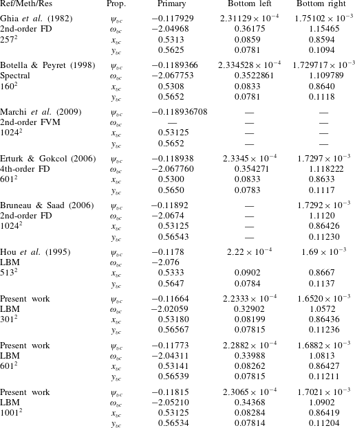
. A choice of relevant published results is listed in table 1. The location of primary and secondary vortex cores is accurate to within
 $0.3\,\%$
of the characteristic length set by the lid. Streamfunction and vorticity at the primary vortex core are slightly less accurate and each deviate by around
 $0.7\,\%$
with the highest resolution tested. While the errors follow a clearly diminishing trend as resolution is increased, residual errors might however persist even at very high resolutions due to corner singularity effects and to the intrinsic compressibility of the LBM, although these remaining inaccuracies are deemed of minor concern for the purposes of the present study. All in all, it can be safely ascertained that the LBM code is properly resolving the benchmark LDSC flow.
Literature review of location of primary and secondary vortices and characteristic properties for LDSC flow at
 $Re=1000$
. Vortex cores (
 $\text{vc}$
) are defined as relative extrema of streamfunction
 $\unicode[STIX]{x1D713}$
.

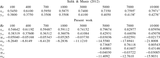
As a further validation, to verify the adequate treatment of boundary conditions on the inclined walls of a triangular enclosure, a few LDTC flow cases have been run and compared to the only available results in the literature on this geometry, reported by Sidik & Munir (Reference Sidik and Munir2012) and listed in table 2. The resolution has been set to
 $601\times 301$
in the horizontal and vertical coordinates, respectively. Sidik & Munir (Reference Sidik and Munir2012) only reported the rightmost vortex location, and yet only with dubious accuracy. However, the agreement is fairly reasonable up to
 $Re=3000$
. As we will show later on, two stable steady solutions coexist at
 $Re=5000$
and
 $Re=7000$
, and the agreement is good if the right branch is selected for comparison. A run at
 $Re=10\,000$
was conducted with the lid in reverse motion, such that the vortex being measured is not the primary one. Comparisons with direct measurements (on the figures, marked with
 $\dagger$
) of primary vortex location provide a fairly good agreement.
Primary vortex location and intensity for LDTC flow as compared to published results of Sidik & Munir (Reference Sidik and Munir2012). The numbers marked with
 $\dagger$
have been measured directly from the figures to correct for evident confusion in choosing the primary vortex.

Lattice Boltzmann models and resolution have been assessed by converging a steady (
 $Re=7000$
), a periodic (
 $Re=8500$
) and a quasi-periodic (
 $Re=9000$
) solution employing classic SRT, iLBM and MRT-iLBM models with resolutions
 $N=601$
,
 $1201$
and
 $2401$
. Cavity centre velocity components and lid centre wall shear stress errors are within
 $1\,\%$
of characteristic values in the cavity. Flow-field visualisations are indistinguishable to the naked eye. Oscillation frequency of time-dependent solutions is however a little off for the lowest resolution and classic model, although the discrepancy does not seem to have an important effect on the dynamics or the location and nature of the bifurcations. Modulational frequency for the quasi-periodic solution is also accurate to around
 $1\,\%$
already for
 $N=601$
and irrespective of the LBM model used. We have observed a slight advantage for the MRT-iLBM model at the lowest resolution as compared to the other two. In accordance with the convergence analysis, the study has been mostly done with the classic LBM model (due to its higher computational efficiency and faster running time) and a resolution
 $N=601$
, although the other two models and higher resolutions have been employed occasionally to verify the validity of the results, which we deem sufficiently accurate (at least qualitatively) up to
 $Re\simeq 14\,000$
.
2.6 Corner singularities versus regularisation
As already mentioned in § 1, cavity flows are singular at the corners. Numerical simulations might be prone to inaccuracies if the issue is not properly addressed, particularly when using high-order space discretisations. Unfortunately, to the authors’ knowledge there exists no straightforward method to deal with corner singularities in the LBM, other than opting for regularisation of the velocity boundary condition. Nonetheless, the method being only second order in space, corner singularities are not expected to have a pivotal impact on bulk flow dynamics. As a matter of fact, some of the literature results presented in table 1 for LDSC flow simply ignored corner singularities with little to no impact whatsoever as to the location and intensity of primary and secondary vortices. It must be borne in mind that ignoring corner singularities does not imply that the corners are truly singular, but that the regularisation is left instead to the practical implementation of the numerical method, which acts implicitly at the fine scale of the grid size (Gonzalez et al. Reference Gonzalez, Ahmed, Kuehnen, Kuhlmann and Theofilis2011). We have however run a few regularised cases in order to assess the inaccuracies introduced by ignoring corner singularities. In particular, we have strongly regularised the lid tangential velocity following
 $$\begin{eqnarray}\boldsymbol{u}(\boldsymbol{x}_{\mathit{l}};t)=([1-(2x-1)^{p}]^{2},0),\end{eqnarray}$$
with
 $p=18$
,
 $32$
and
 $64$
, which attain
 $99\,\%$
of the lid nominal velocity within
 $12.8\,\%$
,
 $7.7\,\%$
and
 $4.0\,\%$
of the lid extent away from the corners, respectively. For
 $N=601$
, the sharp rise from zero at the corner to the
 $99\,\%$
target is resolved with 78, 47 and 25 grid points, respectively. Runs with the SRT model at the same Reynolds numbers used for the grid convergence analysis produced the expected type of solutions in all cases: steady at
 $Re=7000$
, periodic at
 $Re=8500$
and quasi-periodic at
 $Re=9000$
. All monitored variables show a gradual approach towards the singular case as the regularisation parameter
 $p$
is increased. A few additional computations with the highly regularised case (
 $p=64$
) around the Hopf bifurcation confirmed both its existence and nature, albeit slightly shifted in the Reynolds parameter.
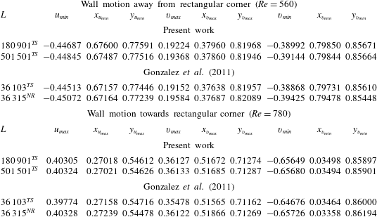
The combined numerical and experimental work of Gonzalez et al. (Reference Gonzalez, Ahmed, Kuehnen, Kuhlmann and Theofilis2011) on the isosceles rectangular triangle with the moving wall adjacent to the right-angled corner provides yet another shot at validating our LBM code. In their analysis, they report accurate results for two steady two-dimensional cases: the wall moving away from the rectangular corner at
 $Re=560$
and towards it at
 $Re=780$
. Their results were obtained using the lid velocity regularisation of (2.19) with
 $p=18$
for several resolutions. We have run the same two cases with the same regularisation but with somewhat higher resolution and compared against their highest-resolution runs. Table 3 reports the minima and maxima of the two components of the velocity field
 $(u,v)$
and their location within the domain. The configuration is such that the origin
 $(x,y)=(0,0)$
is at the acute corner where the left vertical leg meets the hypotenuse, the rectangular corner is at the top left at
 $(x,y)=(0,1)$
and the moving top leg (the lid) meets the hypotenuse at
 $(x,y)=(1,1)$
. Our results at
 $Re=560$
for
 $N=601$
and
 $N=1001$
grid points along the equal-sized legs show adequate convergence with maximum deviations slightly above
 $10^{-3}$
– usually below – and reaching as low as
 $10^{-4}$
in some cases. At
 $Re=780$
, with the wall moving in the opposite direction, mesh convergence is excellent with deviations of the order of
 $10^{-4}$
and sometimes down to
 $10^{-5}$
. Agreement with results reported by Gonzalez et al. (Reference Gonzalez, Ahmed, Kuehnen, Kuhlmann and Theofilis2011) is remarkable, as our values fall systematically within the uncertainty range set by their computations of the same steady states via time-stepping and with a Newton–Raphson solver.
Extrema of the two velocity components
 $(u,v)$
and their location
 $(x,y)$
for the rectangular triangle with the moving wall adjacent to the rectangular corner. Results are compared against those of Gonzalez et al. (Reference Gonzalez, Ahmed, Kuehnen, Kuhlmann and Theofilis2011), using the same exact regularisation with
 $p=18$
in (2.19). Here
 $L=N(N+1)/2$
is the total count of grid points, with
 $N$
the number of grid points along the two equal legs for equispaced meshes (all but the time-stepping results of Gonzalez et al. (Reference Gonzalez, Ahmed, Kuehnen, Kuhlmann and Theofilis2011)). Counts
 $L=180\,901,501\,501,36\,315$
result from
 $N=601,1001,269$
, respectively. The superscripts
 $^{\mathit{TS}}$
and
 $^{\mathit{NR}}$
refer to time-stepping and Newton–Raphson, respectively, as the method for obtaining the solutions.

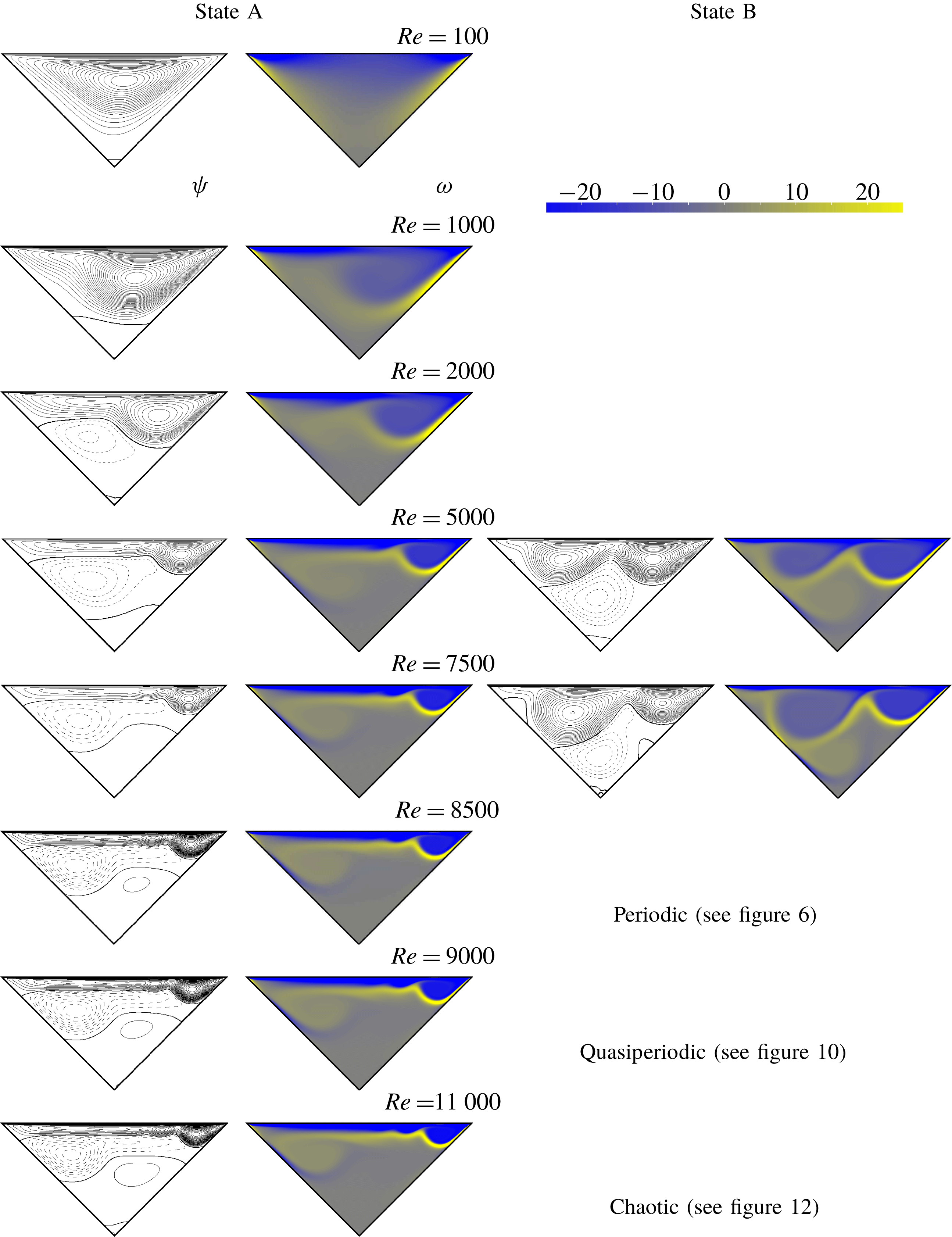
Evolution of the steady states (left: A; right: B) as
 $Re$
is increased from 100 to 7900. Vortical structures are evidenced by the streamline patterns. Vorticity ranges in
 $\unicode[STIX]{x1D714}\in [-25,25]$
, blue (dark) for negative, yellow (bright) for positive, levels as indicated by the colour bar at the top right of the figure (the colour bar is shared by all colour maps in the paper and is therefore not reproduced alongside every and each one of them). Streamfunction isocontours are equispaced in intervals of
 $\unicode[STIX]{x0394}\unicode[STIX]{x1D713}=10$
, solid for negative, dashed for positive and thicker solid lines indicate level 0.

3 Results
A stable steady state, characterised by a domain-filling clockwise vortex, governs the dynamics of the LDTC flow at sufficiently low
 $Re$
. This simple flow topology evolves into more complex vortex arrangements as
 $Re$
is increased. As a matter of fact, the steady base state coexists with another stable steady state within a fairly wide range of flow regimes. While the base state remains steady and stable up to rather large
 $Re$
, this other secondary steady solution undergoes a series of transitions that result in temporally chaotic dynamics. We provide in this section an inventory and characterisation of the different states that arise across a wide
 $Re$
range in the transitional regime.
3.1 Steady states
Figure 3 shows the evolution of the steady base state as
 $Re$
is increased. The morphing of the streamlines indicates that the evolution is anything but uneventful. At very low values of the Reynolds number the solution structure is dominated by a single clockwise vortex, although an incipient secondary vortex of opposite sign begins to emerge already at
 $Re=100$
at the bottom of the cavity. The secondary vortex, of much lower intensity, grows as the primary vortex is pushed towards the right-hand side. The boundary layer deceleration on the upstream wall, observed by Gonzalez et al. (Reference Gonzalez, Ahmed, Kuehnen, Kuhlmann and Theofilis2011) at
 $Re=500$
when the lid moves away from the sharp corner towards the right-angled corner, is clearly visible at
 $Re=1000$
despite the disparity of triangular configurations under consideration. The same phenomenon has been reported by Erturk & Gokcol (Reference Erturk and Gokcol2007) at similar
 $Re$
, for both the equilateral triangular configuration and the isosceles right-angled geometry with the lid moving towards the right-angle. At
 $Re=2000$
, a third smaller vortex has arisen, again at the bottom, that rotates in the same sense as the primary vortex. As this tertiary vortex grows in the bottom of the cavity with a bias towards the right-hand wall, the secondary vortex moves to the left-hand wall while overtaking in size (but not in intensity) the primary vortex and squeezing it against the lid. As a consequence, the primary vortex gets elongated along the top lid and its centre is pushed towards the right-hand wall. The shape of the top vortex is reminiscent of the flow topology found by Erturk & Gokcol (Reference Erturk and Gokcol2007) at equiparable Reynolds numbers for the isosceles right-angled geometry, but this time with the lid moving away from the right-angle. In this respect, our particular geometry seems to share features with the right-angled isosceles triangular cavity where the moving lid is adjacent to the right-angle, when the lid moves in both one direction and the other. A lid sliding away from a sharp angle at low
 $Re$
seems to induce a deceleration or even separation of the boundary layer on the upstream slanted stationary wall. Meanwhile, a lid moving towards a sharp angle tends to push and squeeze the primary (or top) vortex against the lid and elongate it with a downstream bias as
 $Re$
is increased.
From
 $Re\gtrsim 4908$
the three-vortex arrangement base state, henceforth referred to as state A, coexists with another stable solution of conspicuously different flow topology. While the strong vortex on the top right-hand corner persists in this second state, designated hereafter as state B, its size is larger and its tail, which on the base state extended along the lid, has evolved into a new vortex of equal sign (clockwise) that pushes the middle vortex, of opposite sign (anticlockwise), down, forming a strong vortex pair. As a result, an intense jet develops that crosses the cavity following a left-hand down-pointing diagonal through its centre, hits the left wall midway and splits in two. The jet is clearly visible from the high-shear traces it leaves on the vorticity fields and the opposite-sign boundary layers that develop on the left-hand wall at either side from the stagnation point at the impingement location, where the jet splits. Besides the main vortical structure just described, three smaller vortices start nucleating: at the bottom of the cavity, close to the top corner on the left-hand wall and halfway through the right-hand wall. It is this complex steady-vortex pattern, illustrated at
 $Re=5000$
, that undergoes the first bifurcation of time-dependent nature. The jet becomes oscillatory and the stagnation point on the right-hand wall starts moving periodically. From this point on, state B initiates a series of transitions into ever increasingly complex time dependence that eventually leads to chaotic motion. In the meantime, the original base state A persists fairly unaltered as a stable solution for flow regimes in excess of
 $Re\gtrsim 13\,400$
. Beyond this point, it also acquires time-dependency.
The secondary vortex on the left-hand wall that develops early on after the inception of state B seems again to be the result of a lid sliding away from a sharp corner, as it bears strong resemblance to the separation bubble reported by Erturk & Gokcol (Reference Erturk and Gokcol2007) for the isosceles triangular cavity with the lid moving towards the rectangular corner.
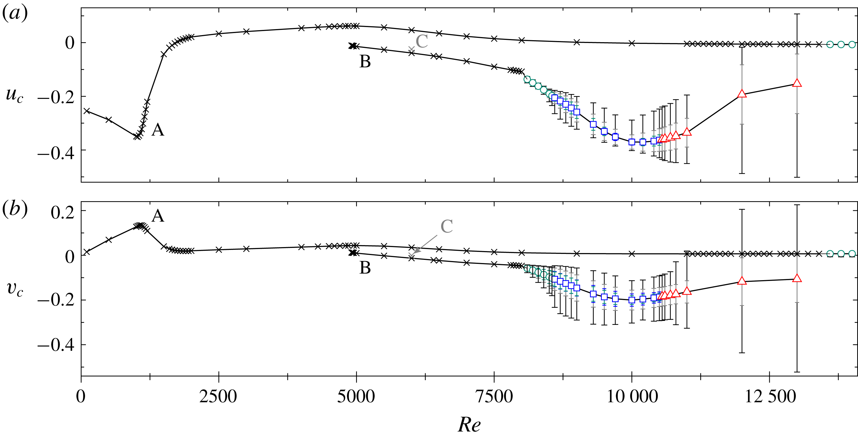
The coexistence of two distinct solution branches is clear from figure 4, where both components of velocity at the centre of the cavity (
 $u_{c},v_{c}$
) have been plotted against
 $Re$
to illustrate the bifurcation diagram for LDTC flow. Steady solutions on the primary (base, A) and secondary (B) branches are marked with crosses. While A-type solutions have nearly quiescent flow at the cavity centre, B-type states feature negative values of both velocity components due to the presence of the diagonal jet. Bistability occurs for the whole range of existence of B-type steady states and no evident branching connecting both types of solutions can be inferred from the bifurcation diagram.
Bifurcation diagram of the LDTC flow. Horizontal (
 $u_{c}$
, top) and vertical (
 $v_{c}$
, bottom) velocity components at the cavity centre as a function of
 $Re$
. The various symbols represent steady solutions (crosses), periodic orbits (circles), quasi-periodic solutions (squares) and chaotic flow (triangles). The outermost error bars span from minimum to maximum, while the inner grey indicate root-mean-square values. Periodic and quasi-periodic solutions include an additional error bar (green) indicating the Fourier spectrum main peak amplitude. The blue error bars for quasi-periodic solutions convey the energy contained in the primary and secondary spectral peaks combined. All solutions are stable except for steady-state C (the isolated grey cross), which has a one-dimensional unstable manifold.

Both types of solutions have been previously reported in the literature, although their dissimilar flow topology has gone widely unnoticed. Sidik & Munir (Reference Sidik and Munir2012) found, in our same triangular geometry, type-A states up to
 $Re\leqslant 3000$
and type-B solutions from
 $Re\geqslant 5000$
on, but the wide
 $Re$
steps they took failed to raise awareness of their distinct nature. In a similar but related geometry – a trapezoidal cavity with height-to-length aspect ratio
 $\unicode[STIX]{x1D6E4}=\sqrt{3}/3\simeq 0.577$
and corner angles of
 $60^{\circ }$
– Zhang et al. (Reference Zhang, Shi and Chai2010) found steady solutions up to
 $Re\leqslant 7500$
that closely resemble our primary branch A-states. The periodic solution they found at
 $Re=8150$
, however, shares common features with our secondary branch B-state. Both the large and small vortex arrangements (exception made of the small vortex at the bottom of our triangular cavity), as well as the diagonal jet across the cavity centre are remarkably evocative of our B-type solution. An analogous explanation in terms of coexistence of solutions might be behind the disagreement found in the literature regarding equilateral triangular cavities. The solution found by Kohno & Bathe (Reference Kohno and Bathe2006) at
 $Re=5000$
would thus be related to state B, while that reported by Pasquim & Mariani (Reference Pasquim and Mariani2008) for
 $Re\geqslant 3000$
seemingly shares features with state A.
3.2 Periodic states
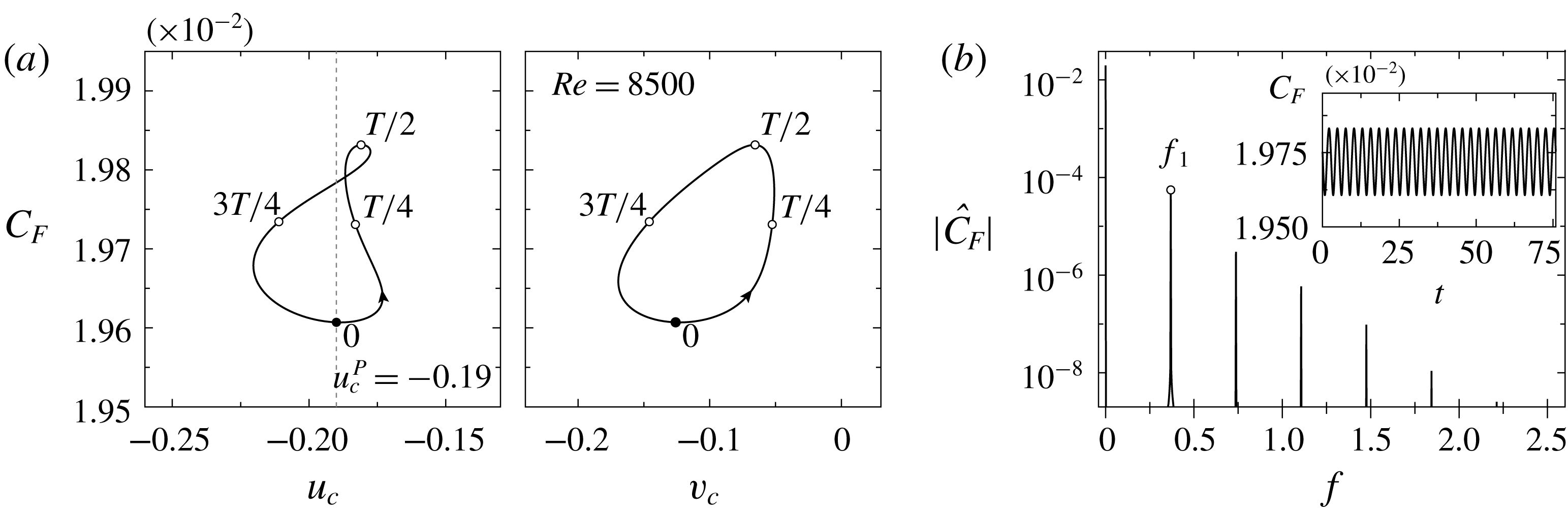
At
 $Re=8500$
the A-type state is no longer stable, but has become unsteady periodic. Figure 5(a) illustrates the phase map trajectory of the periodic orbit through projections on the (
 $u_{c}$
,
 $C_{F}$
) and (
 $v_{c}$
,
 $C_{F}$
) planes. The amplitude of the oscillation is relatively small in terms of
 $C_{F}$
(of the order of
 $1\,\%$
) but quite remarkable when it comes to (
 $u_{c}$
,
 $v_{c}$
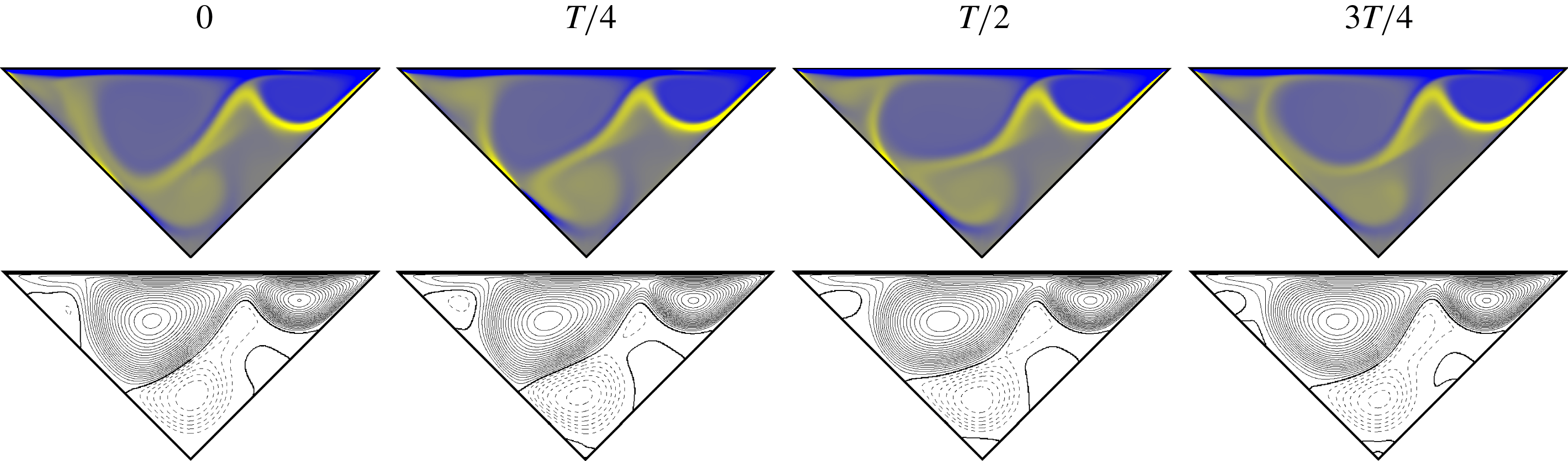
). The reason for this is that the unsteadiness is related to a sweeping motion of the jet, which has a noticeable impact on velocities at the centre of the cavity. The time dependence of the periodic solution is illustrated through four snapshots evenly distributed along a full period in figure 6 (see supplementary movie 1 available at https://doi.org/10.1017/jfm.2019.512). The vortex on the top-right corner of the cavity and the boundary layer on the top lid remain essentially steady, and so does the root of the diagonal jet until about the centre of the cavity. From this point on, the jet describes a sweeping motion that results in a periodic migration of the impingement location on the left-hand wall. The first snapshot (at
 $t_{P}$
, on the Poincaré section) roughly corresponds to the lowest jet arrangement, while the third snapshot (at
 $t_{P}+T/2$
, half a period later) shows the jet at its highest position. The counter-rotating vortices that energise the jet grow and shrink alternately, as shown by the streamfunction isocontours.
B-type periodic orbit at
 $Re=8500$
. (a) Phase map projections on the (
 $u_{c}$
,
 $C_{F}$
) and (
 $v_{c}$
,
 $C_{F}$
) planes. The full circle indicates the fixed point of the Poincaré map defined by
 $u_{c}^{P}=-0.21$
and
 $\dot{u}_{c}>0$
. This together with empty circles indicate snapshots at
 $t-t_{P}=\{0,T/4,T/2,3T/4\}$
in figure 6. (b) Spectrum
 $|{\hat{C}}_{F}|$
of the
 $C_{F}(t)$
signal (inset).


The spectrum of the lid driving-force signal
 $C_{F}(t)$
is represented in figure 5(b) through the modulus of the Fourier transform
 $|{\hat{C}}_{F}(f)|$
of the time series in the inset. A main peak appears at the fundamental frequency
 $f_{1}=0.369$
, which corresponds to a period
 $T=2.71$
. The periodic solution has already evolved nonlinearly away from the bifurcation point, such that clear harmonic peaks can be observed at integer multiples of the fundamental frequency. Nonlinearity is however still weak, as pointed out by the low energy contained in the harmonics as well as by the quasi-sinusoidal shape of the time signal.
Periodic solutions are marked with circles in figure 4. The outermost error bars indicate minimum and maximum values. Root-mean-square values are indicated by the inner grey error bars. The innermost coloured error bars indicate the fundamental spectral peak. All three sets of error bars show the increase of oscillation amplitude with
 $Re$
of the A-type periodic state.
The flow topology and temporal dynamics of the trapezoidal cavity solution in Zhang et al. (Reference Zhang, Shi and Chai2010) at
 $Re=8150$
are perfectly compatible with our periodic solution and both states could probably be related by an appropriate homotopy transformation from one geometry to the other.
It takes a much higher
 $Re$
to destabilise the base steady state A. An A-type periodic solution may however be observed at
 $Re=14\,000$
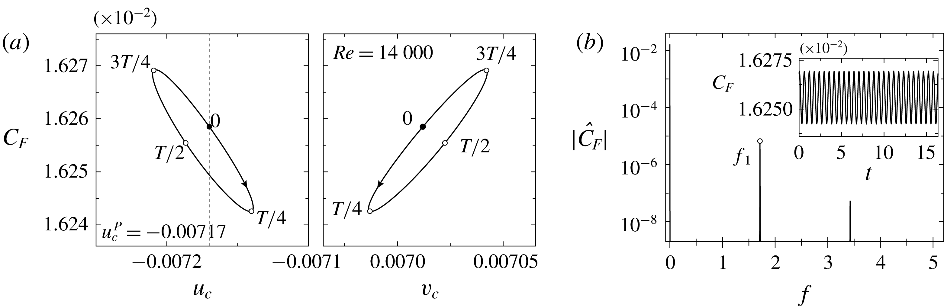
. Figure 7 portrays its temporal dynamics. The oscillation amplitude is considerably weaker in comparison with B-type periodic orbits and is barely perceptible in all three variables used for the phase map projections. The flow at the centre of the cavity is nearly quiescent, and the fundamental frequency,
 $f_{1}=1.719$
, is substantially higher than that for the B-type periodic state, thus indicating a distinct instability mechanism.
A-type periodic orbit at
 $Re=14\,000$
. (a) Phase map projections on the (
 $u_{c}$
,
 $C_{F}$
) and (
 $v_{c}$
,
 $C_{F}$
) planes. The full circle indicates the fixed point of the Poincaré map defined by
 $u_{c}^{P}=-0.00717$
and
 $\dot{u}_{c}>0$
. This together with empty circles indicate snapshots at
 $t-t_{P}=\{0,T/4,T/2,3T/4\}$
in figure 8. (b) Spectrum
 $|{\hat{C}}_{F}|$
of the
 $C_{F}(t)$
signal (inset).

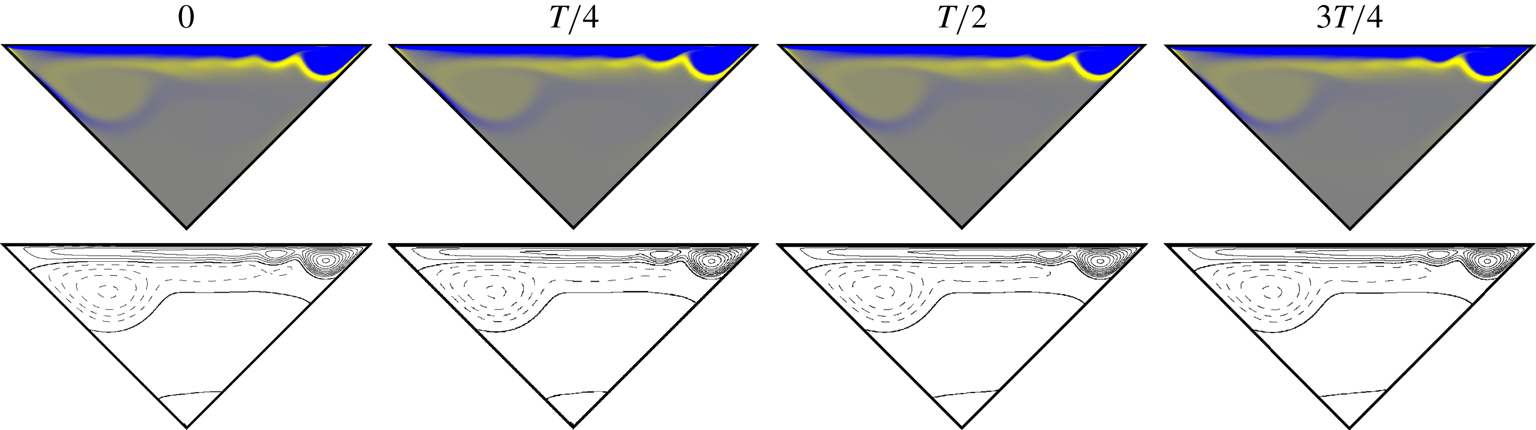
(See supplementary movie 2) Flow-field evolution of the A-type periodic orbit at
 $Re=14\,000$
. Snapshots are taken at four evenly spaced time instants along a full period, starting from a Poincaré crossing, and marked with circles in figure 7(a). Colour codes and line styles as for figure 3.

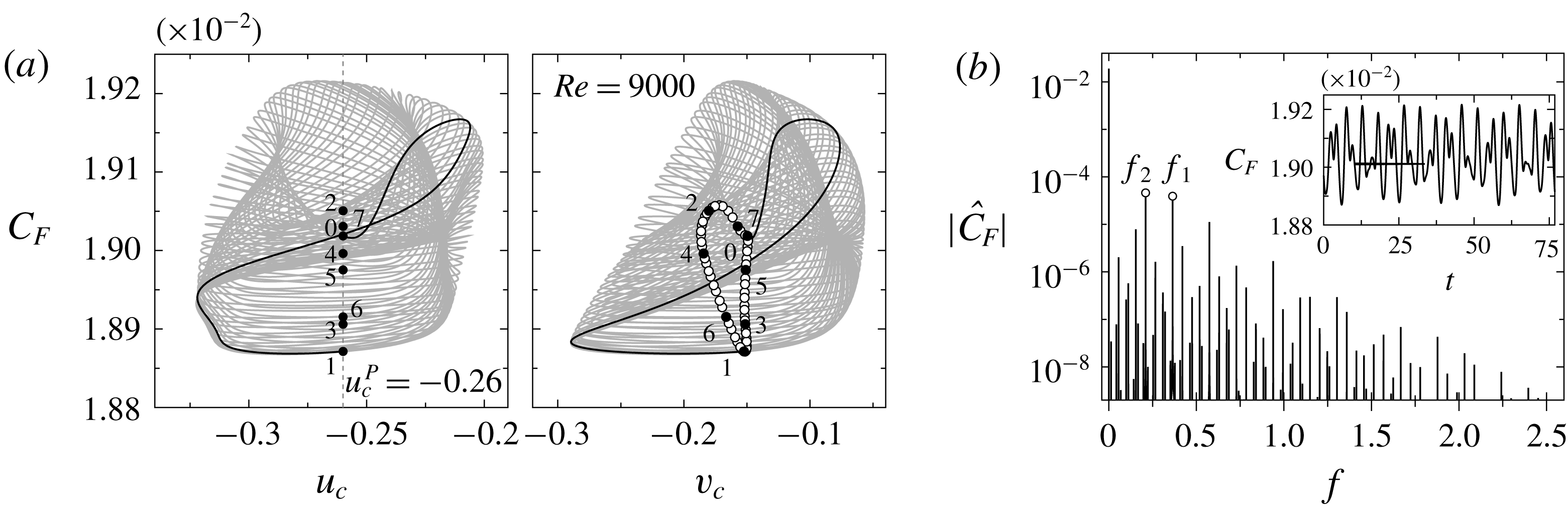
B-type quasi-periodic solution at
 $Re=9000$
. (a) Phase map projections on the (
 $u_{c}$
,
 $C_{F}$
) and (
 $v_{c}$
,
 $C_{F}$
) planes. Empty circles indicate crossings of the Poincaré section defined by
 $u_{c}^{P}=-0.26$
and
 $\dot{u}_{c}>0$
. Numbered full circles correspond to the eight consecutive crossings pictured in figure 10. The solid black line corresponds to one phase map flight between two consecutive crossings. (b) Spectrum
 $|{\hat{C}}_{F}|(f)$
of the
 $C_{F}(t)$
signal (inset).

Figure 8 (see supplementary movie 2) shows four snapshots equispaced along a full period. The flow topology preserves the characteristic elongated primary vortex squeezed against the lid that is characteristic of the A-state. The periodic dynamics corresponds to a wave-type instability that travels leftwards along the interface between the primary and secondary vortices. The instability is so sharply confined to this high-shear region that any one of the snapshots is barely distinguishable from the steady state at sufficiently high
 $Re$
. Only when the snapshots are displayed as a series of frames in a sequence is the time dependence made evident. The wavy dynamics can be ascribed to a Kelvin–Helmholtz instability of the shear layers at either side of the jet that develops parallel (and close) to the wall due to the interaction of the primary and secondary vortices.
3.3 Quasi-periodic states
At
 $Re=9000$
, a second frequency, incommensurate with the original one, has arisen and the B-type solution has evolved into quasi-periodicity. Figure 9(a) depicts phase map trajectories of the quasi-periodic solution as it winds around an invariant torus that has clearly developed into the nonlinear regime. Unlike for the periodic orbit at
 $Re=8500$
, phase map trajectories do not close after each flight between consecutive crossings of the Poincaré section. One such flight has been highlighted (black solid line) for comparison with figure 5(a). The continuous-time quasi-periodic solution shows up in the Poincaré map as a discrete-time limit cycle. The spectrum
 $|{\hat{C}}_{F}|(f)$
of
 $C_{F}(t)$
in figure 9 retains the fundamental frequency peak and harmonics, albeit slightly shifted to
 $f_{1}=0.364$
, of the periodic solution, but incorporates a modulational frequency peak
 $f_{2}=0.21$
. The interaction of the fundamental and modulational frequencies results in a collection of additional peaks at all linear combinations of both frequencies, but the spectrum remains discrete as corresponds to the Fourier transform of a quasi-periodic signal. The new and old frequencies are close to each other, such that no slow–fast dynamics separation becomes evident. Furthermore, the frequencies are incommensurable (their ratio is irrational), which results in phase map trajectories densely filling the invariant torus, as is evident from figure 9(a). Accordingly, the discrete limit cycle of the Poincaré map, indicated with circles in the (
 $u_{c}$
,
 $C_{F}$
) plane, is densely packed.


The rotation number of the solution is given by the frequency ratio
 $R=f_{1}/f_{2}=1.7381$
. The discrete-time limit cycle must be interpreted as winding anticlockwise. Eight consecutive crossings have been numbered and marked with full circles. When the solution evolves from 0 to 1 and then to 2, a complete winding around the limit cycle (and a little more) has been accomplished. A second complete loop results from further evolution up to sometime between crossings 3 and 4. The third loop occurs between crossings 5 and 6. Finally, a fourth winding requires evolving until close to crossing 7, which is past, yet not far from, crossing 0. All in all, slightly less than seven flights to four complete turns around the discrete limit cycle, which corresponds to an approximate rotation number
 $R\simeq 7/4=1.75$
, very close to the exact value given by the frequency ratio.
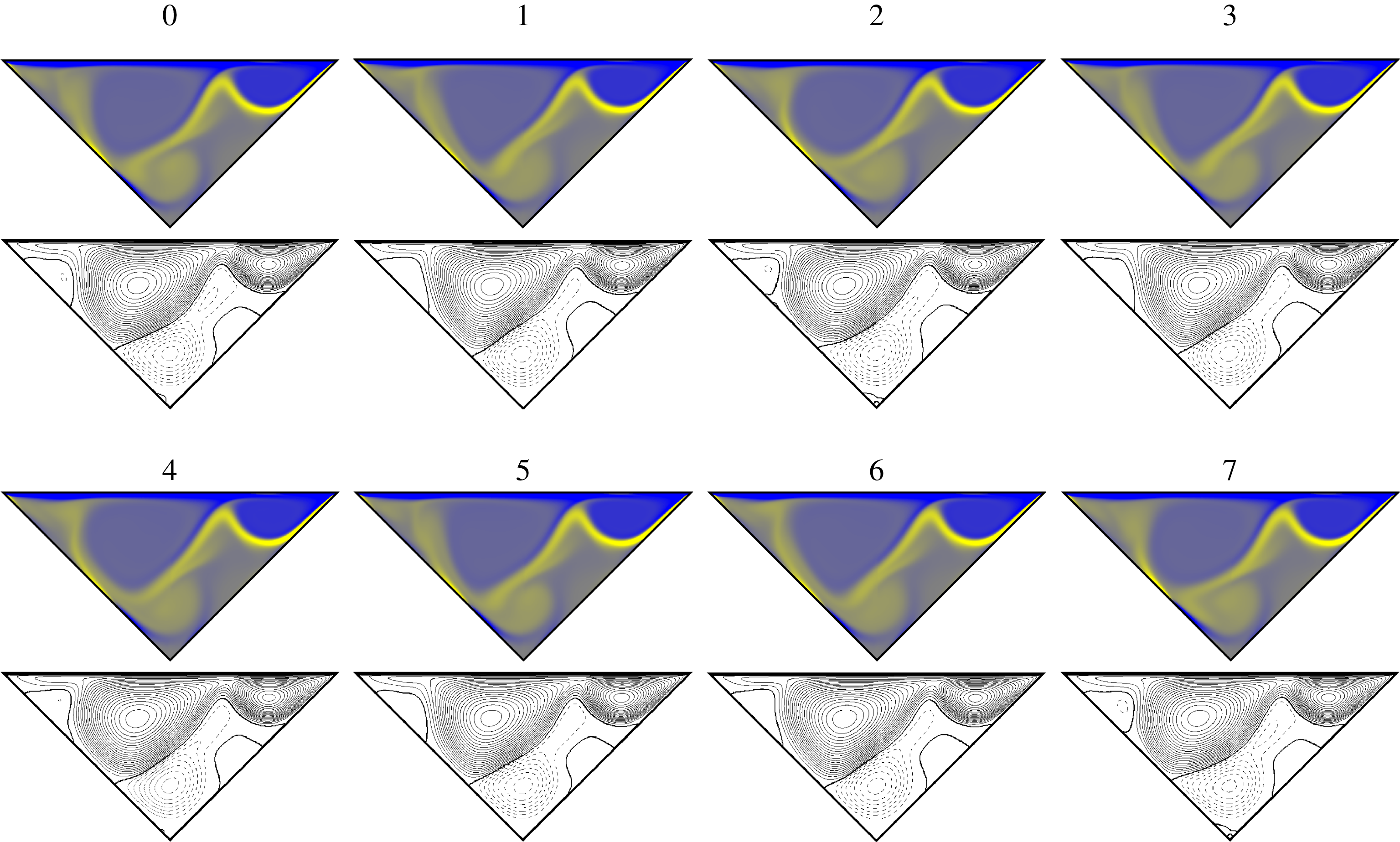
The time dependence of the quasi-periodic solution along each flight between consecutive Poincaré crossings is governed by the same instability mechanisms as those of the periodic solution. The dynamics merely corresponds to the sweeping motion of the jet as already illustrated by figure 6. The added instability is of a modulational nature and its effect is that of modifying the amplitude of the oscillation from cycle to cycle. In order to convey the varying character of the solution, figure 10 (see supplementary movie 3) depicts consecutive crossings of the Poincaré section to allow comparison of the flow fields at equal phase across cycles. All snapshots are fairly similar except for slight variations associated with the modulational instability. The Poincaré sections for
 $Re=8500$
and
 $Re=9000$
have advertently been chosen to roughly capture the solution at the same phase stage, namely when the jet is at its lowest. In this sense, the snapshots in figure 10 can be interpreted as how the lowest jet position of snapshot
 $t-t_{P}=0$
of figure 6 changes from cycle to cycle. Snapshots
 $0$
and
 $7$
are the mutually closest on the discrete-periodic orbit. Snapshots
 $1$
,
 $3$
and
 $6$
(a little less so with
 $5$
), which correspond to low
 $C_{F}$
, are characterised by a slightly downward-bending jet with low impinging point, and a triangular-shaped top-left vortex. Snapshots
 $0$
,
 $2$
and
 $7$
, with higher
 $C_{F}$
, feature more rounded top-left vortices and an upward-bending distal jet. The phase map region represented by snapshot
 $4$
marks an intermediate stage at which the jet is at its straightest.
Quasi-periodic solutions are marked with squares in figure 4. Error bars represent oscillation amplitude in the same way as for periodic solutions. A continuity from periodic to quasi-periodic oscillation amplitude is evidenced, although the increasing trend is contained and even momentarily reversed possibly due to a displacement of the jet location. A fourth coloured set of error bars adds to the fundamental oscillation spectrum peak amplitude, the amplitude of the fundamental modulation peak, to convey the magnitude of the modulational dynamics, which also increases with
 $Re$
.
The allegedly periodic solution that Zhang et al. (Reference Zhang, Shi and Chai2010) report at
 $Re=10\,000$
for the trapezoidal cavity has a recognisable B-type flow topology, and the temporal dynamics, although poorly represented by nearly quiescent cavity centre probe readings, is compatible with a phase-locked quasi-periodic solution.
3.4 Chaotic attractor
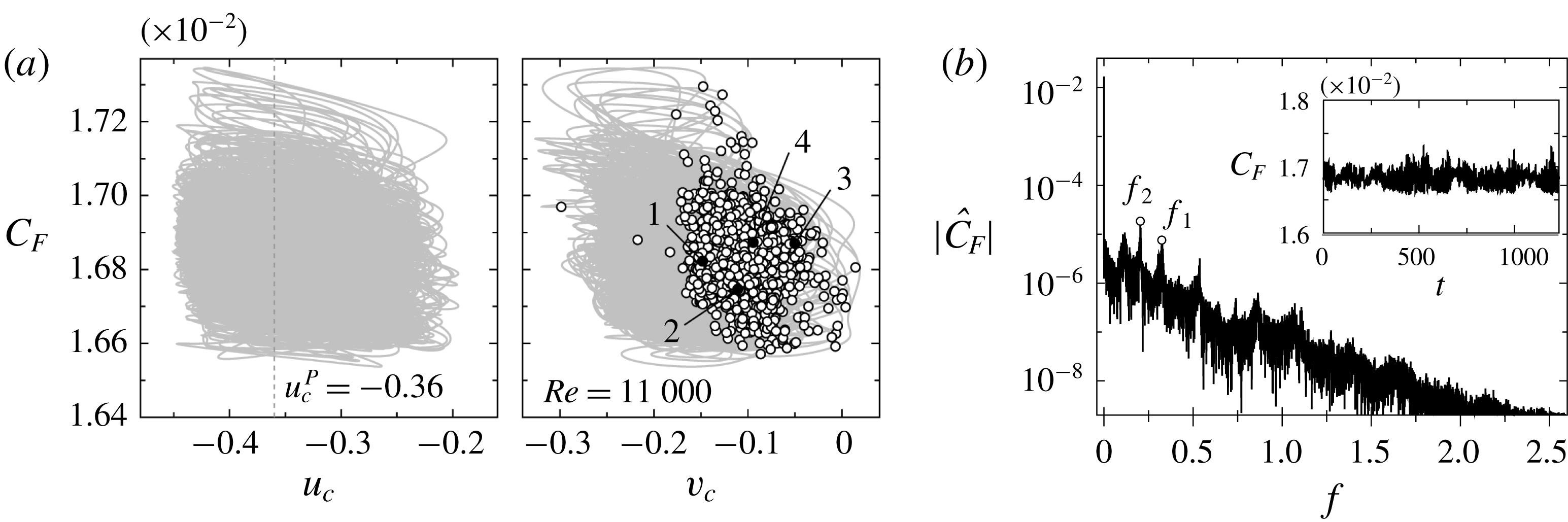
The LDTC flow exhibits B-type chaotic dynamics at
 $Re=11\,000$
, as evident from figure 11. Trajectories seem to wind haphazardly in phase space and pierce the purposely defined Poincaré section at random locations. The dynamics, however, remains confined to a fairly small region in phase space and retains a certain structure that becomes all the more obvious upon examination of the spectrum in figure 11(b). Protruding from the broadband noise that is characteristic of chaotic dynamics, the peaks at the oscillatory (
 $f_{1}$
) and modulational (
 $f_{2}$
) frequencies remain clearly visible. A third peak at
 $f<f_{2}$
might seem to imply the arising of new dynamics, but close inspection reveals that it corresponds to a mere linear combination (
 $f_{1}{-}f_{2}$
) of the two main peaks as a consequence of nonlinear resonant interaction of the oscillatory and modulational dynamics.
B-type chaotic solution at
 $Re=11\,000$
. (a) Phase map projections on the (
 $u_{c}$
,
 $C_{F}$
) and (
 $v_{c}$
,
 $C_{F}$
) planes. Empty circles indicate crossings of the Poincaré section defined by
 $u_{c}^{P}=-0.36$
and
 $\dot{u}_{c}>0$
. Numbered black circles indicate crossings shown in figure 12. (b) Spectrum
 $|{\hat{C}}_{F}|(f)$
of the
 $C_{F}(t)$
signal (inset).

At this
 $Re$
the oscillation of the jet has become violent enough to occasionally break. When this happens, the jet rolls counter-clockwise into a vortex while the boundary layers on the left-hand wall gradually dissipate. When finally shed in an upward whip of the broken jet, the vortex travels, impacts the left-hand wall and recombines with a vortex that is permanently trapped at the bottom of the cavity supplying it with renewed energy. The process is followed by the eventual restitution of the impinging jet. This behaviour is already present at the lower
 $Re=10\,500$
, except that the full process occurs in an orderly manner and repeats periodically (see supplementary movie 4). At
 $Re=11\,000$
, however, the jet roll-up and liberation never repeat at the same phase along the cycle, so that the resulting dynamics is chaotic. Figure 12 (see supplementary movie 5) shows snapshots at four crossings of the Poincaré section defined by
 $u_{c}^{P}=-0.36$
and
 $\dot{u}_{c}>0$
, each one representative of different dynamics that might occur along the chaotic trajectories. The Poincaré crossings shown in both snapshots 1 (
 $t=2.6~\text{s}$
in supplementary movie 5) and 2 (
 $t=12.4~\text{s}$
) are characterised by a large trapped vortex in the bottom corner that forces the jet to bend clockwise halfway in its development and impinge on the wall fairly horizontally. While snapshot 1 corresponds to an almost stagnant phase of the jet, snapshot 2 is followed instead by a mild oscillation. The Poincaré crossing shown in snapshot 3 (
 $t=20.1~\text{s}$
) features a jet that is clearly disrupted and starting to roll up into an incipient counter-clockwise vortex. Following the crossing, the vortex grows and is released in an upward whip of the jet. Once free, the vortex travels towards the wall and pairs up with the trapped vortex at the bottom corner and feeds it with new vorticity. In this process the impinging location slightly diffuses and the boundary layers on the left-hand wall start dissipating until the jet forms back and reestablishes the original flow topology. Snapshot 4 (
 $t=35.4$
) depicts a flow topology very similar to that of snapshots 1 or 2, but in this case the crossing is followed by a violent oscillation and the occurrence of a jet roll-up episode similar to that of snapshot 3.


Chaotic solutions are marked with triangles in figure 4. Fluctuation amplitude rapidly grows with
 $Re$
, as evidenced by both the extrema and root-mean-square error bars.
The similarity to the trapezoidal cavity of Zhang et al. (Reference Zhang, Shi and Chai2010) ends with the quasi-periodic solution. The chaotic solutions they report at
 $Re=12\,500$
and
 $15\,000$
are very different from one another, and of a spatial complexity that we have not come across in our triangular cavity set-up.
4 Discussion
The B-type states that appear along the route from laminar steady flow to chaotic are compatible with a Ruelle–Takens-type scenario (Ruelle & Takens Reference Ruelle and Takens1971; Newhouse et al. Reference Newhouse, Ruelle and Takens1978). In this frame, the steady state is expected to destabilise in a Hopf bifurcation, thereby issuing a branch of periodic states. These would in turn become modulationally unstable in a Neimark–Sacker bifurcation at which quasi-periodic solutions would arise. In the absence of symmetries, two incommensurable frequencies, i.e. quasi-periodic motion on an invariant torus, are generically sufficient to precede transition to chaotic motion. The origin of the B-type flow topology and its ensuing three-step route to chaos will be the object of analysis in this section, and the nature of each one of the bifurcations elucidated.
4.1 The saddle-node bifurcation
Following the B-type steady states branch backwards in Reynolds number, the solution would seem to vanish into thin air at
 $Re_{\mathit{SN}}\simeq 4908$
. A thorough analysis of the transient dynamics reveals that the final decay onto the steady state, while it exists, is exponential and gets slower as
 $Re_{\mathit{SN}}$
is approached. This is suggestive of a real negative eigenvalue gradually advancing towards a zero crossing. Moreover, the last few solutions before the eventual zero crossing are well fitted by a square-root law following
 ${\sim}\sqrt{Re-Re_{\mathit{SN }}}$
. Both facts put together are indicative of a saddle-node bifurcation, whence node (state B) and saddle (henceforth referred to as state C) steady-state solution branches are issued. We choose not to provide a detailed description of the saddle-node bifurcation here, as it adds little value to the discussion, but deem it pivotal instead to produce evidence of the existence of the saddle branch.
As a saddle solution that pairs up with a stable nodal solution, state C possesses a one-dimensional unstable manifold that drives trajectories towards nodal state B on one side and pushes dynamics away from itself on the other. It is therefore not reachable by time evolution but its stable manifold bounds, if only locally, the basin of attraction of state B, and separates it from the basin of attraction of every other existing attractor, in this case state A. We have employed the edge-tracking technique (Skufca, Yorke & Eckhardt Reference Skufca, Yorke and Eckhardt2006) to explore the dynamics on the basin boundary, which in cases like the one at hand is known to eventually converge onto the saddle solution. Thus, starting from the A-type and B-type solutions at
 $Re=6000$
, we have followed a refinement process by picking intermediate initial conditions along a straight line in phase space connecting both states
 $(\boldsymbol{u},p)_{\unicode[STIX]{x1D6FC}}=\unicode[STIX]{x1D6FC}(\boldsymbol{u},p)_{A}+(1-\unicode[STIX]{x1D6FC})(\boldsymbol{u},p)_{B}$
. The refining bisection process on parameter
 $\unicode[STIX]{x1D6FC}$
leads to the determination of neighbouring initial conditions that evolve together on the basin boundary (critical threshold, also known as edge) for very long times before eventually parting, one towards state A, the other towards state B. The refinement can be taken down to machine precision, at which time a new refinement sequence can be started between the last bounding trajectories at a later time. This alternate succession of refinement procedures and adequate time leaps allows for tracking edge trajectories indefinitely.
Figure 13(a) shows the result of three consecutive refinement processes with two intervening time advances (indicated by
 $r_{1}$
and
 $r_{2}$
). The black lines correspond to bounding trajectories obtained from each one of the three bisection refinement processes undertaken, the solid line always finally departing towards state A while the dashed line eventually leaving for state B. The locations of states A and B are indicated with grey dashed lines to guide the eye. The trajectory on the basin boundary clearly converges onto a steady state after some initial rather wild transients and a subsequent gradual oscillatory damping (see the inset) that might be indicative of a possibly oncoming Hopf bifurcation at larger
 $Re$
. In any case, after three refinements and at around
 $t\gtrsim 150$
the steady state can be considered as sufficiently converged. This steady state, which governs the dynamics on the boundary separating the basins of attraction of states A and B, is shown in figure 13(b) and indicated with an empty circle in figure 13(a). Its relative phase-space position with respect to states A and B is marked with an isolated grey cross labelled C in figure 4, in representation of the full branch of unsteady solutions that would be extremely costly to track. State C is similar but not identical to state B. Their resemblance results from their being connected at the saddle-node bifurcation not so far away at
 $Re_{SN}$
, but their nonlinear evolution at larger values of the parameter can be largely independent.
Steady state C, resulting from edge tracking at
 $Re=6000$
between bounding solutions A and B. (a) Time evolution of
 $u_{c}$
for several initial conditions tightly confining the dynamics to the basin boundary. The A- and B-labelled horizontal grey dashed lines indicate states A and B, respectively. Solid (dashed) lines indicate bounding trajectories eventually escaping towards state A (B). The vertical grey dotted lines indicate two successive edge-tracking refinements (labels
 $r_{1}$
and
 $r_{2}$
). The inset shows an extreme magnification of the closest approach to steady-state C resulting from refinement
 $r_{2}$
. (b) Steady-state C, taken at the point along the basin boundary indicated with a circle in panel (a).

4.2 The Hopf bifurcation
A mere inspection of the transients that lead to steady-state B of § 3.1 (sufficiently far from the saddle-node bifurcation) reveals that final asymptotic convergence follows a spiralling trend, as evidenced by the
 $(u_{c}^{\prime },v_{c}^{\prime })$
phase map projection in the inset of figure 14(a). Here the primes denote deviation from steady-state values. This is an indication that the leading eigenmode is a complex-conjugate pair, and that the steady state reduces to a stable focus when the dynamics is projected on the manifold spanned by the leading eigenpair, all other eigendirections contracting faster.
Asymptotic evolution of the perturbation field around the stable steady state. (a) Sequences of
 ${u_{c}^{\prime }}^{P}$
, normalised by
 ${u_{c}^{\prime }}^{P}(0)$
, corresponding to the Poincaré map defined by (4.7) for
 $Re\in [7500,8035]$
. Least-squares fits to the exponential tails are indicated by the grey straight lines. The inset shows, as an example, the phase map that generates the sequence at
 $Re=7500$
. (b) Vorticity (
 $\unicode[STIX]{x1D714}^{\prime }$
, top panel) and streamfunction (
 $\unicode[STIX]{x1D713}^{\prime }$
, bottom panel) on a Poincaré section at
 $Re=8000$
.

The instantaneous flow field can be expressed in terms of the stable steady state
 $(\bar{\boldsymbol{u}},\bar{p})$
plus a perturbation field
 $(\boldsymbol{u}^{\prime },p^{\prime })$
:
 $$\begin{eqnarray}\boldsymbol{u}(\boldsymbol{x};t)=\bar{\boldsymbol{u}}(\boldsymbol{x})+\boldsymbol{u}^{\prime }(\boldsymbol{x};t),\quad p(\boldsymbol{x};t)=\bar{p}(\boldsymbol{x})+p^{\prime }(\boldsymbol{x};t).\end{eqnarray}$$
The equations of motion for the perturbation are obtained by substituting (4.1) in (2.1):
 $$\begin{eqnarray}\left.\begin{array}{@{}c@{}}\unicode[STIX]{x2202}_{t}\boldsymbol{u}^{\prime }+(\boldsymbol{u}^{\prime }\boldsymbol{\cdot }\unicode[STIX]{x1D735})\boldsymbol{u}^{\prime }+(\bar{\boldsymbol{u}}\boldsymbol{\cdot }\unicode[STIX]{x1D735})\boldsymbol{u}^{\prime }+(\boldsymbol{u}^{\prime }\boldsymbol{\cdot }\unicode[STIX]{x1D735})\bar{\boldsymbol{u}}=-\unicode[STIX]{x1D735}p^{\prime }+{\displaystyle \frac{1}{Re}}\unicode[STIX]{x1D6FB}^{2}\boldsymbol{u}^{\prime },\\ \unicode[STIX]{x1D735}\boldsymbol{\cdot }\boldsymbol{u}^{\prime }=0,\end{array}\right\}\end{eqnarray}$$
with homogeneous Dirichlet boundary conditions for
 $\boldsymbol{u}^{\prime }$
.
For sufficiently small perturbation fields of order
 $O(\unicode[STIX]{x1D700})$
with
 $\unicode[STIX]{x1D700}\ll 1$
, i.e. for flow fields at a vanishing distance from the steady state, the perturbation advection term
 $(\boldsymbol{u}^{\prime }\boldsymbol{\cdot }\unicode[STIX]{x1D735})\boldsymbol{u}^{\prime }\sim O(\unicode[STIX]{x1D700}^{2})$
becomes negligible relative to all other terms, which remain of order
 $O(\unicode[STIX]{x1D700})$
, and the equations linearise:
 $$\begin{eqnarray}\left.\begin{array}{@{}c@{}}\displaystyle \unicode[STIX]{x2202}_{t}\boldsymbol{u}^{\prime }+(\bar{\boldsymbol{u}}\boldsymbol{\cdot }\unicode[STIX]{x1D735})\boldsymbol{u}^{\prime }+(\boldsymbol{u}^{\prime }\boldsymbol{\cdot }\unicode[STIX]{x1D735})\bar{\boldsymbol{u}}=-\unicode[STIX]{x1D735}p^{\prime }+{\displaystyle \frac{1}{Re}}\unicode[STIX]{x1D6FB}^{2}\boldsymbol{u}^{\prime },\\ \displaystyle \unicode[STIX]{x1D735}\boldsymbol{\cdot }\boldsymbol{u}^{\prime }=0.\end{array}\right\}\end{eqnarray}$$
The search for solutions of the form
 $(\boldsymbol{u}^{\prime },p^{\prime })(t)=(\tilde{\boldsymbol{u}},\tilde{p})\text{e}^{\unicode[STIX]{x1D706}t}$
results in a generalised constrained eigenproblem
 $$\begin{eqnarray}\left[\begin{array}{@{}cc@{}}\unicode[STIX]{x1D706} & 0\\ 0 & 0\end{array}\right]\left(\begin{array}{@{}c@{}}\tilde{\boldsymbol{u}}\\ \tilde{p}\end{array}\right)=\left[\begin{array}{@{}cc@{}}-(\bar{\boldsymbol{u}}\boldsymbol{\cdot }\unicode[STIX]{x1D735})\diamond -(\diamond \boldsymbol{\cdot }\unicode[STIX]{x1D735})\bar{\boldsymbol{u}}+{\displaystyle \frac{1}{Re}}\unicode[STIX]{x1D6FB}^{2}\diamond & -\unicode[STIX]{x1D735}\diamond \\ \unicode[STIX]{x1D735}\boldsymbol{\cdot }\diamond & 0\end{array}\right]\left(\begin{array}{@{}c@{}}\tilde{\boldsymbol{u}}\\ \tilde{p}\end{array}\right),\end{eqnarray}$$
with eigenmodes
 $(\tilde{\boldsymbol{u}}_{i},\tilde{p}_{i})$
and associated eigenvalues
 $\unicode[STIX]{x1D706}_{i}$
. The dynamics of the linearised problem exactly decouples into the superposition of the evolution of individual eigenmodes:
 $$\begin{eqnarray}(\boldsymbol{u}^{\prime },p^{\prime })(t)=\mathop{\sum }_{i}a_{i}(\tilde{\boldsymbol{u}}_{i},\tilde{p}_{i})\text{e}^{\unicode[STIX]{x1D706}_{i}t}\xrightarrow[{t\rightarrow \infty }]{}a_{1}(\tilde{\boldsymbol{u}}_{1},\tilde{p}_{1})\text{e}^{\unicode[STIX]{x1D706}_{1}t}+\text{c.c.},\end{eqnarray}$$
where
 $a_{i}$
is the projection of the initial perturbation field
 $(\boldsymbol{u}^{\prime },p^{\prime })(0)$
onto mode
 $i$
, and eigenmodes have been sorted by decreasing value of the real part of their associated eigenvalue. For a stable steady state, all eigenvalues have negative real part (
 $\text{Re}(\unicode[STIX]{x1D706}_{i})<\text{Re}(\unicode[STIX]{x1D706}_{1})<0$
), which results in exponential decay along all eigendirections. The asymptotic behaviour of the perturbation for long times tends to align with the leading eigenmode
 $(\tilde{\boldsymbol{u}}_{1},\tilde{p}_{1})$
(the one associated to the eigenvalue with larger real part,
 $\unicode[STIX]{x1D706}_{1}$
), as the dynamics contracts faster in all other eigendirections
 $(\tilde{\boldsymbol{u}}_{i},\tilde{p}_{i})$
(of smaller real part eigenvalues,
 $\unicode[STIX]{x1D706}_{i}$
,
 $i>1$
).
The fully nonlinear evolution towards a stable steady state will experience nonlinear transients that hinder a modal analysis. Once the initial transients have been overcome, however, the dynamics will asymptotically approach the linear regime and the perturbation will align with the leading eigenmode as in the linear case.
For a focus the leading eigenmode is a complex-conjugate pair
 $(\tilde{\boldsymbol{u}}_{1},\tilde{p}_{1})=(\tilde{\boldsymbol{u}}_{1}^{r},\tilde{p}_{1}^{r})\pm \text{i}(\tilde{\boldsymbol{u}}_{1}^{i},\tilde{p}_{1}^{i})$
with eigenvalue
 $\unicode[STIX]{x1D706}_{1}=\unicode[STIX]{x1D706}_{1}^{r}\pm \text{i}\unicode[STIX]{x1D706}_{1}^{i}$
, the
 $r$
and
 $i$
superscripts denoting real and imaginary part, respectively. Hence the c.c. indication denoting complex conjugation in (4.5).
Setting the time origin sufficiently deep into the linear regime, all degrees of freedom follow an exponential oscillating decay towards the stable steady state, with shared frequency (
 $f=\unicode[STIX]{x1D706}_{1}^{i}/2\unicode[STIX]{x03C0}$
) and damping rate (
 $\unicode[STIX]{x1D706}_{1}^{r}$
). For the perturbation field, this decay is towards annihilation. In particular, the perturbation velocity components at the centre of the cavity decay following
 $$\begin{eqnarray}\left.\begin{array}{@{}c@{}}u_{c}^{\prime }(t)=a_{1}\tilde{u} _{c}\text{e}^{(\unicode[STIX]{x1D706}_{1}^{r}+\text{i}\unicode[STIX]{x1D706}_{1}^{i})t}+\text{c.c.}=e_{u}\text{e}^{\unicode[STIX]{x1D706}_{1}^{r}t}\cos (\unicode[STIX]{x1D706}_{1}^{i}t+\unicode[STIX]{x1D713}_{u}),\\ v_{c}^{\prime }(t)=a_{1}\tilde{v}_{c}\text{e}^{(\unicode[STIX]{x1D706}_{1}^{r}+\text{i}\unicode[STIX]{x1D706}_{1}^{i})t}+\text{c.c.}=e_{v}\text{e}^{\unicode[STIX]{x1D706}_{1}^{r}t}\cos (\unicode[STIX]{x1D706}_{1}^{i}t+\unicode[STIX]{x1D713}_{v}),\end{array}\right\}\end{eqnarray}$$
where
 $\text{c.c.}$
denotes complex conjugation and (
 $e_{u}$
,
 $\unicode[STIX]{x1D713}_{u}$
) and (
 $e_{v}$
,
 $\unicode[STIX]{x1D713}_{v}$
), the initial envelope amplitudes and phases of the
 $u_{c}^{\prime }$
and
 $v_{c}^{\prime }$
signals, respectively, are univocally determined by the choice of the time origin through the projection
 $a_{1}$
of the initial flow state onto the leading eigenmode.
In order to estimate the critical value of the Reynolds number at which the Hopf bifurcation takes place (
 $Re_{H}$
) and the frequency at onset of the periodic orbit branch issued from the Hopf point, the leading complex-conjugate eigenpair must be monitored as the parameter, the Reynolds number, is increased towards the bifurcation point. This can be done by comparing the actual behaviour of
 $(u_{c}^{\prime },v_{c}^{\prime })$
with the expected behaviour according to (4.6), using
 $\unicode[STIX]{x1D706}_{1}^{r}$
and
 $\unicode[STIX]{x1D706}_{1}^{i}$
as fitting parameters.
A convenient way of doing so consists of defining a Poincaré section and examining the resulting discrete-time dynamical system. Here we have chosen to define the section as
 ${\mathcal{S}}=\{(\boldsymbol{u}^{\prime },p^{\prime }):v_{c}^{\prime }=0,\dot{v}_{c}^{\prime }<0\}$
. The Poincaré map is then defined as
 $$\begin{eqnarray}\left.\begin{array}{@{}c@{}}{\mathcal{P}}:{\mathcal{S}}\longrightarrow {\mathcal{S}},\\ \boldsymbol{a}^{P}\longmapsto {\mathcal{P}}(\boldsymbol{a}^{P})=\unicode[STIX]{x1D719}_{T^{P}}(\boldsymbol{a}^{P}),\end{array}\right\}\end{eqnarray}$$
where
 $\boldsymbol{a}=(\boldsymbol{u}^{\prime },p^{\prime })$
defines the state of the continuous-time dynamical system (the Navier–Stokes equations),
 $\unicode[STIX]{x1D719}_{\unicode[STIX]{x1D70F}}(\boldsymbol{a})$
is the flow generated by evolving state
 $\boldsymbol{a}$
for a lapse
 $\unicode[STIX]{x1D70F}$
and
 $\boldsymbol{a}^{P}$
is a state on
 ${\mathcal{S}}$
. Repeated application of the map generates a sequence
 $\boldsymbol{a}^{P}(k)$
with associated crossing times
 $t^{P}(k)$
, which are in fact obtained as a post-process of the continuous-time dynamical system evolution by second-order interpolation of
 ${\mathcal{S}}$
-intersections. Flight times between consecutive crossings are then obtained as
 $T^{P}(k)=t^{P}(k)-t^{P}(k-1)$
.
In the linear regime, equation (4.6) anticipates that
 ${\mathcal{S}}$
-crossings will result in the sequence
 $$\begin{eqnarray}\left.\begin{array}{@{}c@{}}t^{P}(k)={\displaystyle \frac{1}{\unicode[STIX]{x1D706}_{1}^{i}}}\left({\displaystyle \frac{\unicode[STIX]{x03C0}}{2}}-\unicode[STIX]{x1D713}_{v}\right)+{\displaystyle \frac{2\unicode[STIX]{x03C0}}{\unicode[STIX]{x1D706}_{1}^{i}}}k=t^{P}(0)+{\displaystyle \frac{2\unicode[STIX]{x03C0}}{\unicode[STIX]{x1D706}_{1}^{i}}}k=t^{P}(0)+T^{P}k,\\ {u_{c}^{\prime }}^{P}(k)=A_{u}\text{e}^{(\unicode[STIX]{x03C0}/2-\unicode[STIX]{x1D713}_{v})(\unicode[STIX]{x1D706}_{1}^{r}/\unicode[STIX]{x1D706}_{1}^{i})+(2\unicode[STIX]{x03C0}/\unicode[STIX]{x1D706}_{1}^{i})\unicode[STIX]{x1D706}_{1}^{r}k}\cos \left({\displaystyle \frac{\unicode[STIX]{x03C0}}{2}}+(\unicode[STIX]{x1D713}_{u}-\unicode[STIX]{x1D713}_{v})\right)={u_{c}^{\prime }}^{P}(0)\unicode[STIX]{x1D707}^{k},\end{array}\right\}\end{eqnarray}$$
with
 $T^{P}(k)=T^{P}=(2\unicode[STIX]{x03C0}/\unicode[STIX]{x1D706}_{1}^{i})$
being the lapse between consecutive crossings and
 $\unicode[STIX]{x1D707}=\text{e}^{T^{P}\unicode[STIX]{x1D706}_{1}^{r}}$
the dominant multiplier (the eigenvalue of the Poincaré map with largest modulus), real positive here, of the stable fixed point of the Poincaré map, coincident in this case, by construction, with the steady state of the Navier–Stokes equations.
It is therefore to be expected that as convergence onto the steady state progresses into the linear regime, the actual sequences will asymptotically approach (4.8). Then,
 $\unicode[STIX]{x1D706}_{1}^{i}$
could be estimated from
 $$\begin{eqnarray}T^{P}=\lim _{k\rightarrow \infty }T^{P}(k)\longrightarrow \unicode[STIX]{x1D706}_{1}^{i}={\displaystyle \frac{2\unicode[STIX]{x03C0}}{T^{P}}}\end{eqnarray}$$
and
 $\unicode[STIX]{x1D706}_{1}^{r}$
might be reckoned from a least-squares exponential fit, for
 $k\rightarrow \infty$
, of the form
 $$\begin{eqnarray}\log \left({\displaystyle \frac{{u_{c}^{\prime }}^{P}(k)}{{u_{c}^{\prime }}^{P}(0)}}\right)=k\log \unicode[STIX]{x1D707}\longrightarrow \unicode[STIX]{x1D706}_{1}^{r}={\displaystyle \frac{1}{T^{P}}}\log \unicode[STIX]{x1D707}.\end{eqnarray}$$
The inset of figure 14(a) indicates with circles, for the sake of illustration, a collection of consecutive
 ${\mathcal{S}}$
-intersections as projected on the
 $(u_{c}^{\prime },v_{c}^{\prime })$
plane for
 $Re=7500$
. The main panel represents, for a range of
 $Re$
below critical, the sequence
 ${u_{c}^{\prime }}^{P}(k)/{u_{c}^{\prime }}^{P}(0)$
as obtained from figures like the one in the inset, conveniently truncated to eliminate most of the initial nonlinear transients. A least-squares fit to the exponential tails provides the multiplier.
Figure 14(b) depicts streamfunction (
 ${\unicode[STIX]{x1D713}^{\prime }}^{P}$
, top panel) and vorticity (
 ${\unicode[STIX]{x1D714}^{\prime }}^{P}$
, bottom panel) fields of the perturbation (
 $\boldsymbol{a}^{P}$
) on a Poincaré crossing well into the linear regime at
 $Re=8000$
. This flow field can be identified with the eigenmode (
 $\tilde{\boldsymbol{a}}^{P}$
) corresponding to the (positive real) dominant eigenvalue
 $\unicode[STIX]{x1D707}$
of the map. It is, at the same time, the imprint on
 ${\mathcal{S}}$
of the dynamics generated by the complex-conjugate eigenpair (
 $\tilde{\boldsymbol{a}}_{1},\tilde{\boldsymbol{a}}_{1}^{\ast }$
) of the continuous-time dynamical system. It is clear from the figure that the incipient instability concentrates in the high-shear regions of the (still stable) steady state. In particular, upcoming unsteadiness seems to originate at the strong jet that crosses the cavity through its centre and within the boundary layers that develop on the left-hand wall at either side of the stagnation point.
Figure 15(a) shows the evolution of the real (
 $\unicode[STIX]{x1D706}_{1}^{r}$
, bottom panel) and imaginary (
 $\unicode[STIX]{x1D706}_{1}^{i}$
, top panel) parts of the leading eigenvalue. The latter is inferred at each
 $Re$
from (4.9) by estimating the asymptotic saturation of
 $T^{P}(k)$
as the steady state is approached, while the former results directly from (4.10).
Hopf bifurcation. (a) Dependence of the real (
 $\unicode[STIX]{x1D706}_{1}^{r}$
, bottom panel) and imaginary (
 $\unicode[STIX]{x1D706}_{1}^{i}$
, top panel) parts of the leading eigenvalue. Quadratic fits of the points at
 $Re\geqslant 7900$
are drawn with grey dash-dotted lines. (b) Force coefficient oscillation amplitude
 $A_{C_{F}}$
versus
 $Re$
of the bifurcated periodic orbit branch. The grey line corresponds to a square-root fit of the five points closest to the saddle node.

As the critical point is approached, the dynamics around the steady state becomes extremely slow. In cases beyond
 $Re>8000$
, reaching the steady state was impractical, so that an approximation was obtained by averaging instead. This poses no problem as long as the estimation is done from averaging sufficiently long time series, preferably including a natural number of Poincaré crossings, already in the linear regime. The fact that the tails remain exponential are a good sign that the eigenvalue can be estimated accurately.
A quadratic fit to the last few points (
 $Re\geqslant 7900$
) of
 $\unicode[STIX]{x1D706}_{1}^{r}(Re)$
provides a means of estimating the critical
 $Re_{H}\simeq 8039.3$
. A second fit for
 $\unicode[STIX]{x1D706}_{1}^{i}(Re)$
to the same points forecasts a frequency
 $f=\unicode[STIX]{x1D706}_{1}^{i}/2\unicode[STIX]{x03C0}=0.377$
for the branch of periodic orbits at onset.
For
 $Re\geqslant 8040$
, the steady state has become unstable and nonlinear evolution produces a branch of periodic orbits. The oscillation frequency at
 $Re=8040$
is
 $f=0.378$
, in good agreement with the critical value for
 $\unicode[STIX]{x1D706}_{1}^{i}$
. The amplitude of the oscillation, however, does not seem to follow the square-root dependency that would be expected from a supercritical Hopf bifurcation. Figure 15(b) shows how the force-coefficient amplitude of the periodic orbits, measured as
 $A_{C_{F}}=C_{F_{\mathit{max}}}-C_{F_{\mathit{min}}}$
, varies with
 $Re$
. Not only does the amplitude fail to vanish at the bifurcation point, but it remains finite for
 $Re<Re_{H}$
disclosing a region of coexistence of the steady and periodic states. The approach to the periodic orbits is extremely slow in this regime, such that the amplitude has not been measured from converged solutions but extrapolated from a power fit of the form
 $$\begin{eqnarray}A_{C_{F}}(k)=A_{C_{F}}+\left(A_{C_{F}}-A_{C_{F}}(0)\right)|\unicode[STIX]{x1D707}|^{k},\end{eqnarray}$$
where
 $A_{C_{F}}$
is the asymptotic value of the orbit amplitude and
 $\unicode[STIX]{x1D707}$
the multiplier (
 $\unicode[STIX]{x1D707}<1$
for stable periodic orbits), to the sequence
 $$\begin{eqnarray}A_{C_{F}}(k)=\max _{t}C_{F}(t)-\min _{t}C_{F}(t),\quad \text{with }t\in [t^{P}(k-1),t^{P}(k)),\end{eqnarray}$$
once the dynamics has reached the linear regime of convergence onto the periodic orbit.
Quasi-static reduction of
 $Re$
along the periodic orbit branch abruptly falls onto the steady-state branch somewhere in the range
 $Re_{FC}\in [8030,8031)$
, which bounds the hysteresis region to
 $Re\in [Re_{FC},Re_{H}]$
. The disappearance of the periodic orbit branch can be explained by the presence of a fold-of-cycles bifurcation, as a square-root fit
 $A_{C_{F}}=A_{C_{F}}^{FC}+\sqrt{Re-Re_{FC}}$
to the five lowest
 $Re$
periodic orbits seems to confirm. The bifurcation occurs at a critical
 $Re_{FC}=8031.0$
with
 $A_{C_{F}}^{FC}\neq 0$
. In a fold-of-cycles, the stable (nodal) branch of orbits collides with an unstable (saddle) branch and the orbits disappear. It is this unstable branch, not reachable by mere time evolution, that presumably connects with the steady state at
 $Re_{H}$
. The Hopf bifurcation is therefore subcritical.
An analogous study of the A-state transition from steady to periodic seems to indicate that a supercritical Hopf bifurcation occurs at
 $Re\simeq 13\,450$
, although a more thorough analysis would be required to pinpoint the exact location of the bifurcation and confirm its supercritical nature.
4.3 The Neimark–Sacker bifurcation
The periodic solutions branch issued from the subcritical Hopf is replaced by quasi-periodic solutions at higher
 $Re$
, as observed in § 3.3. The shared power spectral density peak at
 $f_{1}$
indicates, however, that the latter states might have evolved from the former at a Neimark–Sacker bifurcation. As a matter of fact, periodic states can be observed up to
 $Re\lesssim 8560$
and quasi-periodic states from
 $Re\gtrsim 8570$
on. Figure 16(a) shows phase map projections on the
 $(v_{c},C_{F})$
plane of stable solutions of the map defined with the Poincaré section
 ${\mathcal{S}}=\{(\boldsymbol{u},p):u_{c}=u_{c}^{P}=-0.21,\dot{u}_{c}^{\prime }>0\}$
. Periodic solutions of the Navier–Stokes equations appear as fixed points of the Poincaré map, while quasi-periodic solutions show as discrete periodic orbits. Thus, phase map trajectories are attracted by fixed points (triangles) up to
 $Re\leqslant 8564$
, and by periodic orbits (collection of circles) from
 $Re\geqslant 8565$
on. The scenario is suggestive of a direct relation between both solution branches, as the evolution of the periodic orbit centre follows smoothly from the evolution of the preexisting fixed points location. Also the amplitude of the discrete periodic orbits seems to grow from the zero amplitude of the discrete fixed points as
 $Re$
is increased beyond their onset value, which points to a supercritical nature of the intervening bifurcation.
The Neimark–Sacker bifurcation. (a) Phase map projections on the
 $(v_{c},C_{F})$
plane of the Poincaré maps defined by
 $u_{c}=u_{c}^{P}=-0.21$
,
 $\dot{u}_{c}>0$
. Periodic orbits are represented by triangles while circles denote quasi-periodic solutions. (b) Evolution across the bifurcation of the primary (
 $f_{1},|{\hat{C}}_{F}(f_{1})|$
, circles) and modulational (
 $f_{2},|{\hat{C}}_{F}(f_{2})|$
, squares) peaks in the spectrum of
 $C_{F}(t)$
, relative to their values at the bifurcation point. The grey dash-dotted line and circle correspond to a square-root fit of the modulational amplitude data
 $|{\hat{C}}_{F}(f_{2})|=k\sqrt{|Re-Re_{NS}|}$
and to the location of the bifurcation, respectively.

To establish the connection between both solution branches, the main spectral frequency peaks (
 $f_{1}$
all along,
 $f_{2}$
for the quasi-periodic solutions) have been monitored alongside the amplitude of the solutions as measured by the spectral energy contained in the aforementioned spectral peaks (
 $|{\hat{C}}_{F}(f_{1})|$
and
 $|{\hat{C}}_{F}(f_{2})|$
, respectively). These provide a means of quantifying the solution oscillation amplitude (for both periodic and quasi-periodic solutions) and the amplitude of the modulation of this oscillation (only for quasi-periodic). As shown in figure 16(b) (bottom panel), the oscillation frequency
 $f_{1}$
evolves continuously from the branch of periodic solutions to that of quasi-periodic orbits, which incorporates a modulational frequency
 $f_{2}$
that is incommensurate with
 $f_{1}$
. This places us in the scenario of a supercritical Neimark–Sacker bifurcation. Figure 16(b) (top panel) shows the evolution of the modulational amplitude
 $|{\hat{C}}_{F}(f_{2})|$
(squares). Supercriticality has been tested by attempting a square-root fit
 $|{\hat{C}}_{F}(f_{2})|=k\sqrt{|Re-Re_{NS}|}$
, with
 $k$
and
 $Re_{NS}$
as fitting parameters (grey dash-dotted line). The quality of the fit is remarkable, and provides a fair estimate of
 $Re_{NS}\simeq 8564.8$
at onset with zero modulational amplitude. A quadratic interpolation to the modulational frequency yields
 $f_{2}^{SN}\simeq 0.2106$
. Further quadratic interpolation to the last three data points before the bifurcation, corresponding to periodic solutions, results in
 $f_{1}^{SN}\simeq 0.3673$
and
 $|{\hat{C}}_{F}(f_{1})|\simeq 5.58\times 10^{-5}$
. The main oscillation amplitude remains fairly stable across the Neimark–Sacker point, while the oscillation frequency stops a decreasing trend and starts growing. Meanwhile, the modulational frequency tends to decrease from its value at the bifurcation as
 $Re$
is increased. The frequency ratio at the bifurcation is
 $R_{SN}=f_{1}^{SN}/f_{2}^{SN}\simeq 1.7441$
, not far from that of the quasi-periodic solution of § 3.3.
In order to provide further evidence of the occurrence of a Neimark–Sacker bifurcation and of its subcriticality, the modal decay of perturbations in the linear regime towards the stable periodic solutions has been analysed in a way analogous to that undertaken to elucidate the nature of the Hopf bifurcation in § 4.2. A Neimark–Sacker bifurcation is that of a fixed point of a map (or discrete-time dynamical system) whereby a complex-conjugate pair of eigenvalues crosses the unit circle in the complex plane. The map here is a Poincaré map, and the fixed point is the branch of periodic solutions.
Let
 $(\bar{\boldsymbol{u}},\bar{p})^{P}$
be a stable fixed point of the map (the intersection of the periodic orbit with the Poincaré section
 ${\mathcal{S}}$
) and
 $(\boldsymbol{u},p)^{P}(k)$
the sequence generated by successive application of the map starting from some initial state within the basin of attraction of the fixed point and sufficiently close to it to be considered within the linear regime. The perturbation field will evolve as
 $$\begin{eqnarray}(\boldsymbol{u}^{\prime },p^{\prime })^{P}(k)\equiv (\boldsymbol{u},p)^{P}(k)-(\bar{\boldsymbol{u}},\bar{p})^{P}=\mathop{\sum }_{i}b_{i}(\tilde{\boldsymbol{u}}_{i},\tilde{p}_{i})^{P}\unicode[STIX]{x1D707}_{i}^{k}\xrightarrow[{t\rightarrow \infty }]{}b_{1}(\tilde{\boldsymbol{u}}_{1},\tilde{p}_{1})^{P}\unicode[STIX]{x1D707}^{k}+\text{c.c.},\end{eqnarray}$$
where
 $b_{i}$
is the projection of the initial perturbation on eigenmode
 $(\tilde{\boldsymbol{u}}_{i},\tilde{p}_{i})^{P}$
of eigenvalue
 $\unicode[STIX]{x1D707}_{i}$
. For convenience, the eigenmodes are sorted by decreasing modulus
 $1<|\unicode[STIX]{x1D707}_{1}|<|\unicode[STIX]{x1D707}_{i}|$
. Note that stability of the fixed point implies that all eigenmodes lie within the unit circle in the complex plane. For large
 $k$
, the evolution will align with the dominant (largest modulus) eigenmode
 $\unicode[STIX]{x1D707}_{1}$
.
Individual perturbation degrees of freedom will therefore asymptotically decay as
 $$\begin{eqnarray}y(k)=b_{1}{\tilde{y}}\unicode[STIX]{x1D707}_{1}^{k}+\text{c.c.}=e_{y}r^{k}\cos (k\unicode[STIX]{x1D703}+\unicode[STIX]{x1D713}_{y}),\end{eqnarray}$$
with
 $r$
and
 $\unicode[STIX]{x1D703}$
the modulus and argument of the eigenvalue
 $\unicode[STIX]{x1D707}_{1}=r\text{e}^{\text{i}\unicode[STIX]{x1D703}}$
, and
 $e_{y}$
and
 $\unicode[STIX]{x1D713}_{y}$
the initial envelope amplitude and phase of the
 $y(k)$
sequence. In particular, figure 17(a) depicts, for several values of
 $Re$
approaching the Neimark–Sacker bifurcation from the stable fixed points branch, the decay of the perturbation force coefficient
 $C_{F}^{\prime P}$
and cavity centre vertical velocity
 $v_{c}^{\prime P}$
. The discrete-time origin (
 $k=0$
) has been set well into the linear regime. For ease of visualisation, both quantities have been normalised by their envelope value (
 $e_{C_{F}^{\prime }P}$
and
 $e_{v_{c}^{\prime }P}$
) at
 $k=0$
, obtained from fitting (4.14) to the numerical data. The left-hand panels clearly show how the decay of
 $C_{F}^{\prime P}$
gets progressively less damped as
 $Re$
is increased towards the bifurcation point (top to bottom). It is also apparent how the decay progresses along seven distinct lines, indicating that the map nearly closes (apart from the obvious contraction onto the fixed point) every seven map iterations. The right-hand panels correspond to
 $(v_{c}^{\prime },C_{F}^{\prime })$
phase map projections and both the decay and the discrete quasi-period of seven are clearly evidenced. The labels at
 $Re=8560$
indicate the visit sequence of the seven paths, numbered from
 $0$
to
 $6$
. The phase at every map iteration does not change by
 $\unicode[STIX]{x0394}\unicode[STIX]{x1D719}\sim 2\unicode[STIX]{x03C0}/7$
(or
 $-12\unicode[STIX]{x03C0}/7$
), as one would tend to think, but rather by
 $\unicode[STIX]{x0394}\unicode[STIX]{x1D719}\sim 8\unicode[STIX]{x03C0}/7$
(or
 $-6\unicode[STIX]{x03C0}/7$
). The rotation number is therefore in the vicinity of
 $R=2\unicode[STIX]{x03C0}/\unicode[STIX]{x0394}\unicode[STIX]{x1D719}\sim 7/4=1.75$
(or
 $-7/3=-2.\overline{3}$
). The frequency ratio of the quasi-periodic solution that results from the Neimark–Sacker bifurcation, as well as its winding sign on the invariant torus, suggests that the map iteration must be considered as winding in the anticlockwise direction and that the positive values of
 $\unicode[STIX]{x0394}\unicode[STIX]{x1D719}$
and
 $R$
are the ones to be confronted with continuous-time data. The sign change in the apparent spiral paths (not to be mistaken for the actual winding of the map trajectories) from clockwise at
 $Re=8555$
to anticlockwise at
 $Re=8560$
is the result of traversing a rational rotation number
 $R=1.75$
at
 $Re=8557.5$
, hence the apparent locking, the straight phase map paths and the perfectly exponential discrete-time decay of each of the individual lines.
Modal decay of perturbations in the vicinity of the Neimark–Sacker bifurcation of the Poincaré map defined by
 $u_{c}=u_{c}^{P}=-0.21$
,
 $\dot{u}_{c}>0$
. (a) Discrete-time evolution of
 $C_{F}^{\prime P}$
(left) and phase map projections on the
 $(v_{c}^{\prime },C_{F}^{\prime })$
plane (right) of the linear decay of a perturbation onto the fixed point for several
 $Re<Re_{NS}$
. Here
 $C_{F}^{\prime P}$
and
 $v_{c}^{\prime P}$
have been normalised by envelope amplitude at
 $k=0$
. (b) Evolution of the modulus (
 $r$
, bottom) and argument (
 $\unicode[STIX]{x1D703}$
, top) of the dominant eigenvalue
 $\unicode[STIX]{x1D707}_{1}=r\text{e}^{\text{i}\unicode[STIX]{x1D703}}$
of the stable fixed point as the bifurcation is approached. Values of
 $r$
and
 $\unicode[STIX]{x1D703}$
are estimated from fits to the numerical data. Grey circles indicate the Neimark–Sacker bifurcation as estimated from quadratic fits to the rightmost few points.

Fitting (4.14) to the
 $C_{F}^{\prime P}$
data at several values of
 $Re$
approaching the Neimark–Sacker bifurcation from the stable fixed points side provides an accurate estimation of the modulus
 $r$
and argument
 $\unicode[STIX]{x1D703}$
of the dominant eigenvalue of the Poincaré map. Their
 $Re$
dependence is shown in figure 17(b). The intersection with the (
 $r=1$
)-line of a quadratic fit to the modulus of the last few points before the bifurcation (bottom panel, dash-dotted grey line) yields an estimate of
 $Re_{NS}\simeq 8565.0$
for the critical point, in good agreement with the value inferred from the modulational amplitude of the quasi-periodic solution resulting from the bifurcation. A second quadratic fit, this time to the argument of the same last few points that precede the Neimark–Sacker bifurcation (top panel, dash-dotted grey line), results in
 $\unicode[STIX]{x1D703}_{NS}\simeq 3.6023$
. The corresponding rotation ratio is
 $R_{NS}\simeq 1.7442$
, again in very close agreement with that obtained from estimating the oscillation and modulational frequencies at the bifurcation point.
4.4 Nonlinear evolution of the two-torus
Figure 18 depicts phase map projections of quasi-periodic (and occasionally phase-locked) solutions winding on the two-torus created at the Neimark–Sacker bifurcation. The hole in the torus is clearly perceptible in the (
 $u_{c}$
,
 $C_{F}$
) projection of the solution at
 $Re=8600$
(black), where nonlinearity is still mild and trajectories retain the most salient features of the underlying periodic orbit that has become unstable in the Neimark–Sacker bifurcation. As
 $Re$
is increased (increasingly lighter shades of grey), the torus evolves nonlinearly, the lid shear force decreases and the dynamics associated with the modulation gains prominence as the imprint on the solution behaviour becomes comparable to that of the oscillation dynamics. Despite the deep transformation of the solution (as evident from phase map projections) from its origin at
 $Re=8600$
to
 $Re=10\,500$
, at the verge of becoming chaotic, the evolution is gradual and uneventful, with the sole exception of a collection of frequency-locking episodes.
Nonlinear evolution of the two-torus. Phase map projections on the (
 $u_{c}$
,
 $C_{F}$
), (
 $v_{c}$
,
 $C_{F}$
) and (
 $v_{c}$
,
 $u_{c}$
) planes of quasi-periodic solutions winding on the two-torus at
 $Re=8600$
,
 $9000$
,
 $9500$
,
 $10\,000$
and
 $10\,500$
(from black toward increasingly lighter shades of grey).

We have detected several such episodes, characterised by the locking of trajectories onto periodic solutions winding on the torus, as the
 $Re$
path in parameter space crosses a series of Arnold tongues. When entering these regions, a fold of cycles occurs on the torus. The periodic solutions observed correspond to the nodal orbit, which pairs up with a saddle orbit that is not detectable through mere time evolution. Both periodic orbits collide and are destroyed in a second fold of cycles upon leaving the Arnold tongue. Phase-locking with frequency ratios 5:3, 21:13, 50:31 or 97:60 has been found at
 $Re=10\,200$
,
 $10\,500$
(lightest grey in figure 18; see supplementary movie 4 for time evolution of vorticity field),
 $10\,540$
and
 $10\,590$
, respectively. In particular, the phase-locked orbit in the tongue at
 $Re\simeq 10\,540$
undergoes a period-doubling cascade that triggers chaotic dynamics.
4.5 The onset of chaotic dynamics
The onset of chaotic motion appears to follow the breakdown of the two-torus created in the Neimark–Sacker bifurcation much in the way advanced by Ruelle & Takens (Reference Ruelle and Takens1971) and later extended by Newhouse et al. (Reference Newhouse, Ruelle and Takens1978). The Afraimovich–Shilnikov theorem postulates three different ways whereby this may occur (Afraimovich & Shilnikov Reference Afraimovich and Shilnikov1983), namely (1) breakdown following some ordinary bifurcation of phase-locked limit cycles; (2) sudden transition in the presence of a homoclinic (or heteroclinic) structure; and (3) soft transition due to a gradual loss of smoothness. All three alternative paths have since been confirmed as naturally occurring in autonomous physical systems (Anischenko, Safonova & Chua Reference Anischenko, Safonova and Chua1993). While the latter path entails direct transition, the former two scenarios involve torus breakdown prior to the advent of chaos, either by the appearance of a period-doubled limit cycle that no longer lies on the invariant torus (first case) or by manifold tangles (second case).
Figure 19 shows phase map projections on the (
 $v_{c}$
,
 $C_{F}$
) plane of the Poincaré map defined by
 ${\mathcal{S}}=\{(\boldsymbol{u},p):u_{c}=u_{c}^{P}=-0.36,\dot{u}_{c}^{\prime }>0\}$
. The phase portrait at
 $Re=10\,520$
(figure 19
a) is clearly indicative of quasi-periodic motion on the two-torus, as the crossings fill the discrete-time limit cycle densely. Its
 $C_{F}$
spectrum is that of a quasi-periodic signal, with clear peaks at the two incommensurate frequencies and a bunch of secondary peaks due to nonlinear effects. At
 $Re=10\,530$
, the system has crossed into a phase-locked region with a 51:30 resonance, meaning that a phase-locked limit cycle of frequency
 $f_{l}=f_{1}/51=f_{2}/30$
is now winding on the invariant torus (figure 19
b). This periodic orbit, visible as a discrete number of crossings on the Poincaré section and with a spectrum made of peaks at all integer multiples of
 $f_{l}$
, corresponds to the stable solution. Pairing up with it, a saddle limit cycle, also winding on the torus, exists. Its unstable manifold, which drives the flow towards the stable limit cycle, fulfils the closure of the invariant set. The torus is still intact. The invariant torus breaks down some place between
 $Re=10\,530$
and
 $Re=10\,540$
, precisely at the period-doubling bifurcation that produces the period-doubled limit cycle we observe at
 $Re=10\,540$
(figure 19
c). The Poincaré map now clearly depicts a period-two discrete limit cycle that, unlike the discrete cycle at
 $Re=10\,530$
, winds twice before closing. The spectrum is conspicuously similar, except for the fact that new peaks have appeared between every two consecutive peaks of the original cycle, the basic frequency having been halved to
 $f_{l_{2}}=f_{1}/102=f_{2}/60$
. A bifurcation cascade, whose detailed analysis is beyond the scope of this study, follows, such that at
 $Re=10\,550$
the solution is no longer periodic but chaotic (figure 19
d). The crossings on the Poincaré section do not fall on precisely located points or along well-defined lines, but now fill a narrow band around the phase-space region where the initial period-doubled cycle appeared. The invariant set has now turned into a strange attractor. The principal peaks and their nonlinearly generated secondary counterparts are still discernible in the spectrum, but they are now accompanied by broadband noise that is well above machine precision and can by no means be ascribed to numerical truncation error.
Onset of chaotic motion. Phase map projections on the (
 $v_{c}$
,
 $C_{F}$
) of the Poincaré map defined by
 $u_{c}^{P}=-0.36$
(left) and spectrum
 $|{\hat{C}}_{F}|$
(right) at (a)
 $Re=10\,520$
, (b)
 $Re=10\,530$
, (c)
 $Re=10\,540$
and (d)
 $Re=10\,550$
.

As it happens, the chaotic transition is reversed as
 $Re$
is increased and a new phase-locked limit cycle corresponding to a different Arnold tongue is obtained at
 $Re=10\,590$
. Increasing
 $Re$
further, the region is left behind following a new period-doubling cascade similar to the one already described. At
 $Re=10\,600$
the flow is again chaotic and no evidence of reverting to quasi-periodicity has been found all the way up to
 $Re=13\,000$
, although this is difficult to ascertain without undertaking a thorough analysis of the evolution of the strange attractor. The evolution from the well-structured mildly chaotic attractor at
 $Re=10\,600$
towards the seemingly unstructured wild attractor at
 $Re=11\,000$
and beyond is gradual, as shown in figure 20. The vestiges of the original torus are progressively lost in an apparently featureless cloud of Poincaré crossings (figure 20
a) and the broadband noise in the spectrum steadily grows in energy (figure 20
b), gradually burying the characteristic frequency peaks.
Evolution of the chaotic set. (a) Phase map projections on the (
 $v_{c}$
,
 $C_{F}$
) of the Poincaré map defined by
 $u_{c}^{P}=-0.36$
and (b) spectrum
 $|{\hat{C}}_{F}|$
(right) at
 $Re=10\,600$
(black),
 $Re=10\,800$
(dark grey) and
 $Re=11\,000$
.

4.6 Bursting events away from the chaotic set
As the chaotic dynamics of the strange attractor becomes progressively wild, bursting episodes start occurring for
 $Re\gtrsim 12\,000$
(see supplementary movie 6) that take phase-space trajectories into a previously unexplored region where some kind of unstable state seems to dwell. These visits become recurrent and protracted as
 $Re$
approaches
 $13\,000$
. The left-hand panel of figure 21 compares the dynamics at
 $Re=13\,000$
(black) and
 $Re=11\,000$
(light grey) by displaying part of the respective
 $u_{c}$
time series. Mean value and fluctuations share similar characteristics part of the time, but regular excursions towards lower
 $|u_{c}|$
values that were absent at
 $Re=11\,000$
occur frequently at
 $Re=13\,000$
. One such excursion is indicated in the time series (dark grey) and zoomed in in the inset. The dynamics in this region seems to be governed by a periodic orbit that captures phase map trajectories along its stable manifold for a while before the solution escapes back following its unstable manifold. The pseudo-periodic nature of the signal is evident in the inset within the inset, which corresponds to a further zoom to the smoothest stage of the excursion. Phase map projection on the (
 $u_{c},v_{c}$
) plane (right-hand panel of figure 21) shows how the chaotic set remains pretty much in the same location where it was at
 $Re=11\,000$
(shown in light grey). However, phase map trajectories clearly incorporate frequent visits to phase-space regions not previously explored, following bursting events (one such event is highlighted in dark grey) that take the dynamics away from the location of the original chaotic set and then back. Especially significant is the occasional wandering at the top-right corner of the phase map, magnified in the inset, where trajectories seem to shadow the unstable manifold of some sort of mildly unstable state, possibly the continuation to this higher
 $Re$
of the state C presented in § 4.1, which would have undergone a Hopf bifurcation at some point earlier in Reynolds number. For a while, the flow in the centre of the cavity stays nearly quiescent, an indication that the diagonal jet that is characteristic of B-type states is momentarily dismantled. The most quiet stage of the approach is shown in the second inset, where two full pseudo-periods have been indicated (black) to convey the dynamic properties of the underlying state that trajectories appear to orbit for a while. We conjecture that the aforementioned state-C saddle solution might be responsible for piercing the chaotic attractor at a slightly higher
 $Re$
in a boundary crisis. We shall not explore the issue further, as the resolution and the computational resources required to fully clarify the situation are well beyond the scope of this study, but leave it for future investigation.
Chaotic flow dynamics at
 $Re=13\,000$
(black), as compared to
 $Re=11\,000$
(light grey). The left-hand panel contains
 $u_{c}$
time series, while the right-hand panel displays phase map projections on the (
 $u_{c},v_{c}$
) plane. A prototypical excursion (dark grey) is highlighted in both panels and the dashed boxes are zoomed in in the respective insets. A further zoom, shown in the second set of insets, reveals the pseudo-periodic nature of the signal in the region of phase space visited during burst events.

5 Conclusions
Evolving in time the equations of fluid motion with a lattice Boltzmann approach, we have unfolded the bifurcation sequence that leads to chaotic dynamics of the incompressible two-dimensional flow within a right-angled isosceles triangular enclosure driven by the tangential motion of its hypotenuse. The steady solutions branch that originates at zero Reynolds number (Stokes flow limit) remains stable for a wide range of flow regimes. This base state (state A) acts as a global attractor up to
 $Re\simeq 4908$
, at which point a second branch of steady solutions (state B) emerges in a saddle-node bifurcation, pairing up with a branch of saddle solutions (state C). The nodal stable solution, characterised by an intense jet diagonally crossing the cavity, becomes unstable in a slightly subcritical Hopf bifurcation at
 $Re\simeq 8040$
, whereby a branch of periodic solutions is issued. Time dependence comes in the form of a periodic oscillation of the jet, and due to the subcritical character of the bifurcation, the solutions are unstable at onset. They become stable, and therefore accessible through time evolution, in a fold of cycles, thus leaving a small range of coexistence of steady and oscillating jet solutions. A second incommensurate frequency arises in a supercritical Neimark–Sacker bifurcation at
 $Re\simeq 8565$
, rendering the dynamics quasi-periodic. The jet remains oscillatory, but the oscillation amplitude incorporates a modulation. As
 $Re$
is further increased, the quasi-periodic solution traverses a series of Arnold tongues. The frequency-locking episode that occurs in the vicinity of
 $Re\simeq 10\,530$
is different from all preceding episodes in that the phase-locked periodic orbit undergoes a period-doubling cascade that results in the emergence of a strange attractor at
 $Re\simeq 10\,550$
. This transition path to chaotic dynamics, one of the three possible torus-breakdown scenarios advanced by Afraimovich & Shilnikov (Reference Afraimovich and Shilnikov1983), is however shortly reversed at slightly higher
 $Re$
before a second transition of the same nature leaves the flow chaotic from
 $Re\gtrsim 10\,600$
on. The dynamics progressively becomes ever more involved and the broadband noise in the spectrum steadily increases, gradually masking the underlying characteristic frequency peaks.
The saddle solution that pairs up with the stable node that undergoes the aforementioned bifurcation cascade does not seem to be related or connected to the base state branch (be it the steady base flow or any of the subsequent bifurcated descendants that take over for
 $Re\gtrsim 13\,450$
), as this latter has been continued and shown to remain an attractor until at least
 $Re<28\,000$
(note that the computations are probably not sufficiently well resolved at these high
 $Re$
). It is nonetheless possible that the saddle state may be playing a crucial role in governing the chaotic attractor dynamics and eventually puncturing and morphing it into a chaotic repeller or saddle.
Acknowledgements
B.A.’s research was financed by the Chinese Scholarship Council (CSC). This work was also supported by the Spanish and Catalan governments under grants FIS2016-77849-R and 2017-SGR-00785, respectively. Part of the computations were done in the Barcelona Supercomputing Centre under grants FI-2017-2-002, FI-2017-3-0009 and FI-2016-3-0038.
Supplementary movies
Supplementary movies are available at https://doi.org/10.1017/jfm.2019.512.