
1 Introduction
Hydrodynamic interaction, arising from the existence of multiple particles in a fluid, plays a significant role in particle motion and the bulk properties of suspension under the inertia of both particles and fluid. The simplest model is a two-dimensional (2-D) flow containing 2-D circular cylinders of equal size and density. This has been the commonly simulated model because of its convenience. Feng, Hu & Joseph (Reference Feng, Hu and Joseph1994) reproduced the drafting–kissing–tumbling (DKT) phenomenon for sedimentation of two circular cylinders in a vertical channel through direct simulations at a terminal Reynolds number  $Re_{T}$ of 70 (
 $Re_{T}=U_{T}d/\unicode[STIX]{x1D708}$, where
 $U_{T}$ is the particle terminal velocity, d is the particle diameter and
 $\unicode[STIX]{x1D708}$ is the fluid kinematic viscosity). DKT motion was first observed by Fortes, Joseph & Lundgren (Reference Fortes, Joseph and Lundgren1987) in an experiment involving the sedimentation of two spheres, which results from the hydrodynamic interaction between spheres at finite fluid inertia. This plays an important role in the evolution of clusters for a sedimentation system with a large number of particles (Fornari, Ardekani & Brandt Reference Fornari, Ardekani and Brandt2017). Aidun & Ding (Reference Aidun and Ding2003) did a numerical study on the sedimentation of two circular cylinders in a narrow channel using the lattice Boltzmann method (LBM). This simple system exhibited a variety of dynamical features when
 $Re_{T}$ varied from 2 to 6. In particular, the periodic state of the cylinders bifurcated into a chaotic state through periodic doubling as
 $Re_{T}$ increased. The same system was later revisited by Verjus et al. (Reference Verjus, Guillou, Ezersky and Angilella2016) for an extended range of
 $Re_{T}$ (1–10). They established a link between the terminal Reynolds number and the non-dimensional driving force using a global diagram. Yacoubi, Xu & Wang (Reference Yacoubi, Xu and Wang2012) simulated the dynamics of a horizontal array of settling cylinders at an intermediate Reynolds number, focusing on the effect of hydrodynamic interaction on settling patterns. Different patterns were found for odd-numbered and even-numbered arrays (Yacoubi et al. Reference Yacoubi, Xu and Wang2012). Similar work was done by Nie, Lin & Zheng (Reference Nie, Lin and Zheng2014), who studied the influence of inter-particle distance on the DKT process. Recently, Nie, Lin & Chen (Reference Nie, Lin and Chen2016) reported grouping behaviour of multiple cylinders settling along their line of centres in a narrow channel at finite Reynolds numbers. They showed that the settling cylinders separated into several groups according to particle–particle interaction, with each group sedimenting at the same rate. Furthermore, they found that this grouping behaviour strongly depended on the number of cylinders as well as the Reynolds number. More recently, simulations were done on the sedimentation of two circular cylinders with different densities at finite Reynolds numbers (Nie, Lin & Gao Reference Nie, Lin and Gao2017; Nie & Lin Reference Nie and Lin2019). This sedimentation system shows two types of periodic state as the Galileo number increases, with different amplitudes and frequencies that also change differently with increasing density difference between cylinders (Nie et al. Reference Nie, Lin and Gao2017; Nie & Lin Reference Nie and Lin2019). In particular, simulations reveal a discontinuous change in the settling velocity of the cylinders as well as in the oscillation period of the cylinders at a critical density difference (Nie & Lin Reference Nie and Lin2019). A possible mechanism behind this discontinuity was also found.
Accordingly, attention has also been paid to three-dimensional (3-D) configurations of this system. Several authors have addressed the role of fluid inertia on the interaction between spheres. Kulkarni & Morris (Reference Kulkarni and Morris2008) simulated the motion of a pair of neutrally buoyant spheres in simple shear flow at finite Reynolds numbers. The closed relative trajectories predicted by the Stokes equations (Batchelor & Green Reference Batchelor and Green1972) are not seen in the presence of fluid inertia, as shown by Kulkarni & Morris (Reference Kulkarni and Morris2008). Instead, two new patterns of particle motion appear, namely, the reversing and spiralling patterns, as a result of the loss of fore–aft symmetry in the Stokes flow. Using an arbitrary Lagrangian–Eulerian technique, Mukundakrishnan, Hu & Ayyaswamy (Reference Mukundakrishnan, Hu and Ayyaswamy2008) simulated the motion of two spheres in a confined rotating flow at intermediate Reynolds numbers. They reported pedalling motion for the two interacting spheres. Furthermore, Cao et al. (Reference Cao, Chen, Li, Liu, Zha, Bao and Zheng2015) simulated the dynamics of two spheres settling in a container at  $Re_{T}\sim O(100)$. They identified hydrodynamic interaction between the spheres in three different regimes (repulsion, attraction and transition) depending on the initial arrangement of the spheres (Cao et al. Reference Cao, Chen, Li, Liu, Zha, Bao and Zheng2015). Dash & Lee (Reference Dash and Lee2015) revisited the DKT phenomenon for
 $Re_{T}$ between 10 and 60 through 3-D simulations as well as experiments, and found new features in the motion of spheres and the flow. Particularly, they reported an inverse DKT pattern that differed from the normal pattern in the rotation direction of the turning couple during tumbling. Recently, the clustering behaviours of dilute suspensions of settling spheres (Huisman et al. Reference Huisman, Barois, Bourgoin, Chouippe, Doychev, Huck, Morales, Uhlmann and Volk2016) and oblate ellipsoids (Fornari et al. Reference Fornari, Ardekani and Brandt2017) were studied for Galileo numbers Ga from 110 to 310 and for Ga fixed at 60, respectively. Both studies showed that the particle settling velocity could be greatly enhanced under conditions where particle clusters formed columnar-like structures (Huisman et al. Reference Huisman, Barois, Bourgoin, Chouippe, Doychev, Huck, Morales, Uhlmann and Volk2016; Fornari et al. Reference Fornari, Ardekani and Brandt2017). The mechanism behind this is not completely understood. However, as pointed out by Huisman et al. (Reference Huisman, Barois, Bourgoin, Chouippe, Doychev, Huck, Morales, Uhlmann and Volk2016), the vertical alignment of particles is primarily caused by the interaction between particles and wakes at intermediate Reynolds numbers where the fluid inertia is significant. Fornari et al. (Reference Fornari, Ardekani and Brandt2017) also found that the hydrodynamic interactions overcome the hindering effect of suspension (Yin & Koch Reference Yin and Koch2007) and increase the settling velocity.
By contrast, studies on flow dynamics resulting from interacting spheres of unequal sizes or densities are nearly limited to the Stokes regime (Darabaner & Mason Reference Darabaner and Mason1967; Davis Reference Davis1969; Batchelor & Green Reference Batchelor and Green1972; Wacholder & Sather Reference Wacholder and Sather1974; Adler Reference Adler1981; Chang & Powell Reference Chang and Powell1993; Navardi, Bhattacharya & Wu Reference Navardi, Bhattacharya and Wu2015). For instance, Wacholder & Sather (Reference Wacholder and Sather1974) predicted the relative trajectories of two unequal spheres settling under gravity in a fluid using the Stokes equations for negligible particle inertia. An interesting phenomenon in this system is the periodic motion of a larger but lighter sphere in the ‘no-escape’ region near a smaller but heavier sphere under certain conditions. Similarly, Adler (Reference Adler1981) theoretically studied relative motion of two spheres of unequal sizes in simple shear flow at zero Reynolds number. That study showed that the smaller sphere may pass over the larger one (open trajectories) or rotate around it (closed trajectories) depending on the initial distance between them, which is consistent with the observation by Darabaner & Mason (Reference Darabaner and Mason1967) and the theory developed by Batchelor & Green (Reference Batchelor and Green1972). Adler (Reference Adler1981) also presented a method to determine the ‘separation surface’, which is the boundary of the region occupied by closed trajectories. Note that the motion of ‘closed trajectories’ has not been found for two equal spheres. In particular, the pedalling motion of two equal spheres in a confined rotating flow (Mukundakrishnan et al. Reference Mukundakrishnan, Hu and Ayyaswamy2008) may not exist when the spheres have different sizes or densities. Mukundakrishnan et al. (Reference Mukundakrishnan, Hu and Ayyaswamy2008) showed that in rotating flow the lighter sphere approaches its equilibrium position while the heavier one undergoes circular motion about its equilibrium position. The primary reason is that the lighter sphere experiences a different wake perturbation from that experienced by the heavier one. Similarly, the hydrodynamic interaction between spheres with unequal sizes also differs much from that between spheres with equal sizes, leading to disappearance of pedalling motion (Mukundakrishnan et al. Reference Mukundakrishnan, Hu and Ayyaswamy2008). Despite the efforts in this area, the hydrodynamic interaction between unequal spheres in the finite-Reynolds-number regime is far from understood, which motivates the present study.
In order to shed light on the interactions between particles, a two-particle system is usually adopted in the numerical framework because it rules out irrelevant factors to a large extent and will be possible to account for the features of a many-particle system. Previous 2-D studies (Aidun & Ding Reference Aidun and Ding2003; Verjus et al. Reference Verjus, Guillou, Ezersky and Angilella2016) showed that this simple system reflects a rich and complex dynamical feature at low but finite Reynolds numbers even for two equal particles, suggesting that the inertia of the system plays a key role in determining the patterns of sedimentation behaviour. A small difference between the densities of particles can be treated as a perturbation of the system, which has been shown to have significant effects on the physics and dynamics of the system in the presence of fluid inertia (Nie et al. Reference Nie, Lin and Gao2017; Nie & Lin Reference Nie and Lin2019). However, studies of this problem for the 3-D case, which has a wider range of engineering applications, are very rare. It is expected that the extra dimension allows different patterns of particle motion and new features of a fluid–particle system to exist. Therefore, as a follow-up of our previous paper (Nie et al. Reference Nie, Lin and Gao2017; Nie & Lin Reference Nie and Lin2019), we focus on the interactions between unequal spheres through simulating a sedimentation system containing two spheres confined in a square tube in this work. As a first step towards understanding this general case, we currently consider spheres with different densities but the same size. The effects of inertia on the motion of the spheres are examined by adjusting the value of Galileo number ( $5\leqslant Ga\leqslant 25$), which results in a Reynolds number range of
 $0.8\leqslant Re_{T}\leqslant 17.3$ for the system. This
 $Re_{T}$ range is comparable to those of previous 2-D studies (Aidun & Ding Reference Aidun and Ding2003; Verjus et al. Reference Verjus, Guillou, Ezersky and Angilella2016; Nie et al. Reference Nie, Lin and Gao2017; Nie & Lin Reference Nie and Lin2019). In particular, the present system is the same as the one used in our recent work (Nie & Lin Reference Nie and Lin2019) if the dimensionality is not taken into consideration, which makes it possible to provide a direct comparison with 2-D computations in a similar
 $Re_{T}$ range. This is the second purpose of the present study. It is well known that 2-D simulations are commonly used to serve as a tool of studying the features of a 3-D system in view of the low computational cost, which, however, raises an inevitable question for us: to what extent is the 2-D system similar to its 3-D counterpart or under what conditions do the 2-D particles behave essentially the same as the 3-D ones? To answer this question a quantitative comparison is needed. We believe that the comparison is helpful to improve the understanding of the effect of dimensionality on the interactions between particles at finite inertia. Note that for the present system the width of square tube is chosen as five times the diameter of the spheres, resulting a moderate confinement ratio of 5. This ratio allows the spheres to hydrodynamically interact with each other in the tube without frequent collisions with the walls to a great extent. Moreover, such confinement ratio means a small 3-D computation domain which enables us to accurately solve the present problem at an affordable computational cost.
The outline of this paper is as follows. The numerical method, flow geometry and boundary conditions are described in § 2. In § 3 we simulate sedimentation of a single sphere as well as two spheres in a box, and compare the results with published data to validate our computational code. Numerical results are presented and discussed in § 4. In this section, six sedimentation patterns are identified for the spheres, and a possible mechanism is discussed. We also quantitatively compare the 2-D and 3-D cases in this section. In § 5 some concluding remarks are given.
2 Method and problem
2.1 Lattice Boltzmann method
In this work the fluid motion is solved through a 3-D lattice Boltzmann method. The discrete lattice Boltzmann equations of a single-relaxation-time model are expressed as (Qian Reference Qian1992)
 $$\begin{eqnarray}f_{i}(\boldsymbol{x}+\boldsymbol{e}_{i}\unicode[STIX]{x0394}t,t+\unicode[STIX]{x0394}t)-f_{i}(\boldsymbol{x},t)=-{\displaystyle \frac{1}{\unicode[STIX]{x1D70F}}}[f_{i}(\boldsymbol{x},t)-{f_{i}}^{(0)}(\boldsymbol{x},t)],\end{eqnarray}$$
where  $f_{i}(\boldsymbol{x},t)$ is the distribution function for the microscopic velocity
 $\boldsymbol{e}_{i}$ in the
 $i$th direction,
 $f_{i}^{(0)}(\boldsymbol{x},t)$ is the equilibrium distribution function,
 $\unicode[STIX]{x0394}t$ is the time step of the simulation,
 $\unicode[STIX]{x1D70F}$ is the relaxation time and
 $w_{i}$ are weights related to the lattice model. The fluid density
 $\unicode[STIX]{x1D70C}$ and velocity
 $\boldsymbol{u}$ are determined by the distribution function
 $$\begin{eqnarray}\unicode[STIX]{x1D70C}=\mathop{\sum }_{i}f_{i},\quad \unicode[STIX]{x1D70C}\boldsymbol{u}=\mathop{\sum }_{i}f_{i}\boldsymbol{e}_{i}.\end{eqnarray}$$
For the 19-velocity model in three dimensions (D3Q19) lattice model used here, the discrete velocity vectors are
 $$\begin{eqnarray}\boldsymbol{e}_{i}=\left\{\begin{array}{@{}ll@{}}(0,0,0)c & i=0,\\ (\pm 1,0,0)c,(0,\pm 1,0)c,(0,0,\pm 1)c & i=1{-}6,\\ (\pm 1,\pm 1,0)c,(\pm 1,0,\pm 1)c,(0,\pm 1,\pm 1)c & i=7{-}18,\end{array}\right.\end{eqnarray}$$
where  $c=\unicode[STIX]{x0394}x/\unicode[STIX]{x0394}t$, and
 $\unicode[STIX]{x0394}x$ is the lattice spacing. The speed of sound is determined through
 $c_{s}=c/\sqrt{3}$. Following Qian (Reference Qian1992), the equilibrium distribution function is chosen as
 $$\begin{eqnarray}{f_{i}}^{(0)}(\boldsymbol{x},t)=w_{i}\unicode[STIX]{x1D70C}\left[1+{\displaystyle \frac{3\boldsymbol{e}_{i}\boldsymbol{\cdot }\boldsymbol{u}}{c^{2}}}+{\displaystyle \frac{9(\boldsymbol{e}_{i}\boldsymbol{\cdot }\boldsymbol{u})^{2}}{2c^{4}}}-{\displaystyle \frac{3\boldsymbol{u}^{2}}{2c^{2}}}\right],\end{eqnarray}$$
where the weights are set to be  $w_{0}=1/3,w_{1{-}6}=1/18$ and
 $w_{7{-}18}=1/36$.
By performing a Chapman–Enskog expansion, the macroscopic mass and momentum equations in the low-Mach-number limit can be recovered
 $$\begin{eqnarray}\displaystyle & \displaystyle {\displaystyle \frac{\unicode[STIX]{x2202}\unicode[STIX]{x1D70C}}{\unicode[STIX]{x2202}t}}+\unicode[STIX]{x1D735}\boldsymbol{\cdot }(\unicode[STIX]{x1D70C}\boldsymbol{u})=0, & \displaystyle\end{eqnarray}$$
 $$\begin{eqnarray}\displaystyle & \displaystyle {\displaystyle \frac{\unicode[STIX]{x2202}(\unicode[STIX]{x1D70C}\boldsymbol{u})}{\unicode[STIX]{x2202}t}}+\unicode[STIX]{x1D735}\boldsymbol{\cdot }(\unicode[STIX]{x1D70C}\boldsymbol{u}\boldsymbol{u})=-\unicode[STIX]{x1D735}p+\unicode[STIX]{x1D707}\unicode[STIX]{x1D6FB}^{2}\boldsymbol{u}. & \displaystyle\end{eqnarray}$$
In this method, the fluid viscosity is computed using  $\unicode[STIX]{x1D708}=c_{s}^{2}\unicode[STIX]{x0394}t(\unicode[STIX]{x1D70F}-0.5)$. For simplicity, both the lattice spacing and time step are set to be 1 in the simulations, i.e.
 $\unicode[STIX]{x0394}x=\unicode[STIX]{x0394}t=1$, unless otherwise stated.
2.2 Boundary conditions
The LBM usually needs a special treatment for a moving boundary to ensure the no-slip boundary condition on the surface of a particle. In this work, we use an improved bounce-back scheme proposed by Lallemand & Luo (Reference Lallemand and Luo2003). This scheme was demonstrated to be stable, robust and easy to implement in the simulations of lattice Boltzmann equations (Lallemand & Luo Reference Lallemand and Luo2003).
The force and torque exerted on the solid particle by the fluid-boundary nodes are computed through the momentum exchange method (Mei et al. Reference Mei, Yu, Shyy and Luo2002; Lallemand & Luo Reference Lallemand and Luo2003). In addition, to account for the effect of a solid particle entering or leaving the fluid, the method proposed by Aidun, Lu & Ding (Reference Aidun, Lu and Ding1998) is used to calculate the added force and torque due to the covered and uncovered fluid nodes. Using the net force and torque, the motion of a particle is determined by solving the Newton equations.
2.3 Collision model
When two particles come into close contact with each other, the lubrication force becomes significant. This force, caused by the attenuation of the fluid film in the gap between the two particles, is repulsive upon approach and attractive upon separation of the particles. However, when the gap between the two particles is of the order of one lattice spacing, the lubrication force is not completely resolved with the LBM. To solve this problem, we use the lubrication-force model proposed by Nguyen & Ladd (Reference Nguyen and Ladd2002):
 $$\begin{eqnarray}\boldsymbol{F}_{\text{lub}}=\left\{\begin{array}{@{}ll@{}}0 & h>h_{c},\\ -6\unicode[STIX]{x03C0}\unicode[STIX]{x1D70C}\unicode[STIX]{x1D708}{\displaystyle \frac{{a_{1}}^{2}{a_{2}}^{2}}{(a_{1}+a_{2})^{2}}}\left({\displaystyle \frac{1}{h}}-{\displaystyle \frac{1}{h_{c}}}\right)^{3/2}(\boldsymbol{U}_{12}\boldsymbol{\cdot }\hat{\boldsymbol{R}}_{12})\hat{\boldsymbol{R}}_{12} & h<h_{c}.\end{array}\right.\end{eqnarray}$$
Here,  $a_{1}$ and
 $a_{2}$ are the radii of the two particles;
 $\boldsymbol{U}_{12}=\boldsymbol{U}_{1}-\boldsymbol{U}_{2}$;
 $h=|\boldsymbol{R}_{1}-\boldsymbol{R}_{2}|-(a_{1}+a_{2})$ is the distance between the particle surfaces; and
 $h_{c}$ represents the cutoff distance between the particle surfaces for the added lubrication force, which is fixed at
 $h_{c}=1.2\unicode[STIX]{x0394}x$ in the simulations. The unit vector is defined by
 $\hat{\boldsymbol{R}}_{12}=\boldsymbol{R}_{12}/|\boldsymbol{R}_{12}|$. Equation (2.7) can be adjusted slightly to account for the particle–wall collision. By doing so we use
 $\boldsymbol{U}_{2}=0$, and
 $\boldsymbol{R}_{2}$ is the corresponding point on the wall.
2.4 Problem
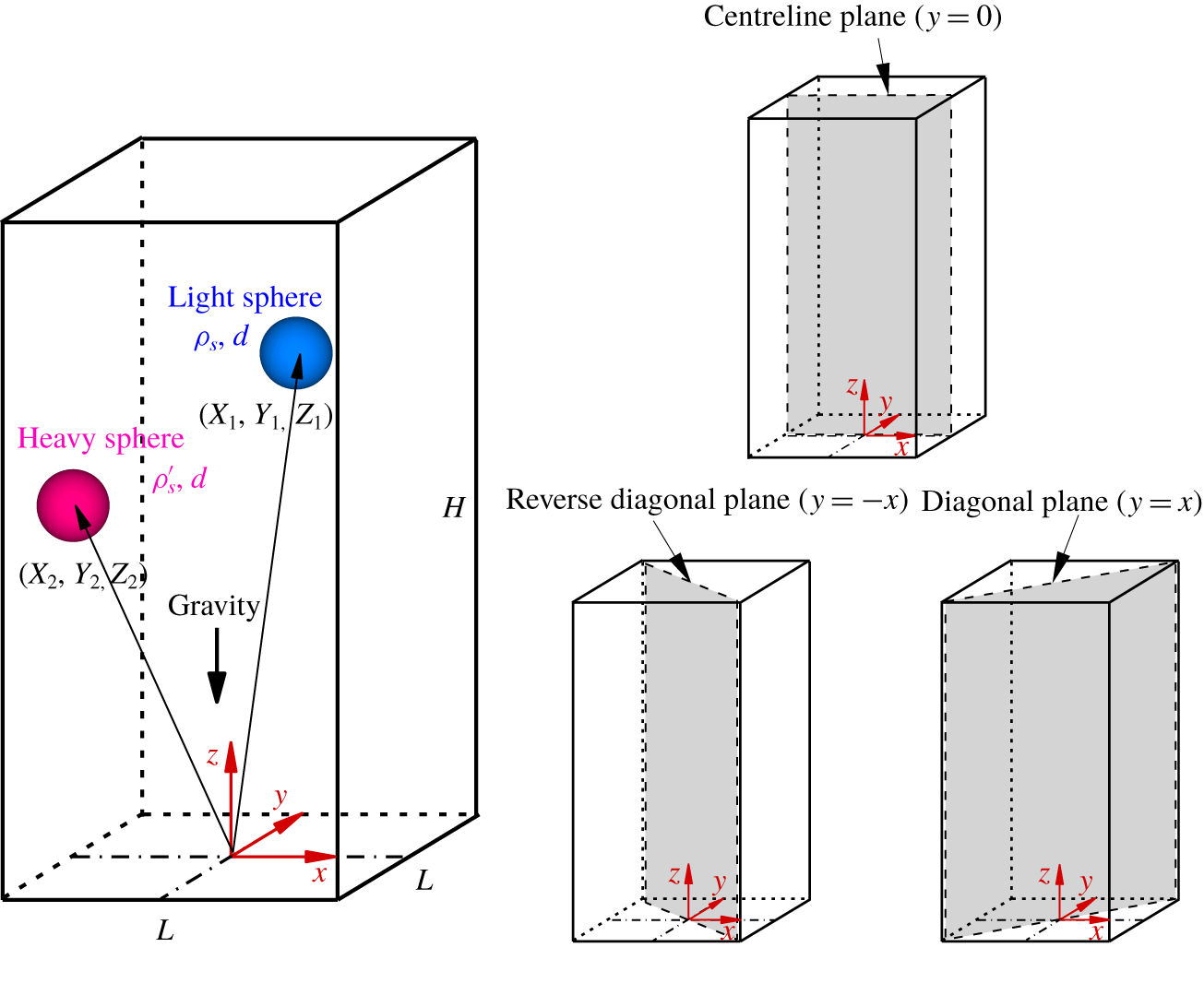
We consider the motion of two interacting spheres during sedimentation in a square tube. As illustrated in figure 1, two spheres of diameter d are released from rest in a square tube filled with a fluid of density  $\unicode[STIX]{x1D70C}$ and kinematic viscosity
 $\unicode[STIX]{x1D708}$. The densities of the spheres are denoted as
 $\unicode[STIX]{x1D70C}_{s}^{\prime }$ (heavy) and
 $\unicode[STIX]{x1D70C}_{s}$ (light). The tube width is typically chosen as
 $L=5d$ and its height as
 $H=30d$. Note that the centreline plane of the tube as well as the (reverse–) diagonal plane is also indicated in figure 1. To simulate an infinite tube, a moving domain is used. Doing this shifts the fluid field and particle positions up by one lattice spacing once the heavy sphere falls below a height of 10d from the bottom boundary. This ensures that the top boundary is always 20d away from the heavy sphere. No-slip boundary conditions are imposed for all tube walls. The normal derivative of the velocity is zero at the upper boundary, and the velocity at the bottom boundary is zero.
Schematic diagram of double-sphere sedimentation in a square tube. The computational domain size is fixed at  $L\times L\times H=5d\times 5d\times 30d$. The centreline plane (
 $y=0$), the diagonal plane (
 $y=x$) and the reverse–diagonal plane (
 $y=-x$) are indicated. The particle positions are designated as
 $X$ (horizontal),
 $Y$ (lateral) and
 $Z$ (vertical). We use the subscripts 1 and 2 to denote the light and the heavy sphere, respectively. The light sphere is initially located at
 $[X_{1}(0),Y_{1}(0),Z_{1}(0)]=[d,0,10d]$ and the heavy one is located at
 $[X_{2}(0),Y_{2}(0),Z_{2}(0)]=[-d,0,10d]$. Both spheres are released from rest in the centreline plane.

As in our previous studies (Nie et al. Reference Nie, Lin and Gao2017; Nie & Lin Reference Nie and Lin2019), the parameter  $\unicode[STIX]{x1D6FC}$ denotes the density difference between the two spheres
 $$\begin{eqnarray}\unicode[STIX]{x1D6FC}={\displaystyle \frac{\unicode[STIX]{x1D70C}_{s}^{\prime }-\unicode[STIX]{x1D70C}_{s}}{\unicode[STIX]{x1D70C}}}.\end{eqnarray}$$
The Galileo number Ga is introduced to control the ratio of the gravitational force to the viscous force and is given by (Jenny, Dušek & Bouchet Reference Jenny, Dušek and Bouchet2004; Dash & Lee Reference Dash and Lee2015)
 $$\begin{eqnarray}Ga=\sqrt{\left({\displaystyle \frac{\unicode[STIX]{x1D70C}_{s}}{\unicode[STIX]{x1D70C}}}-1\right){\displaystyle \frac{gd^{3}}{v^{2}}}},\end{eqnarray}$$
where g is the acceleration due to gravity. Because the terminal velocity of spheres cannot be prescribed, the reference velocity is instead taken as
 $$\begin{eqnarray}U_{0}=\sqrt{\left({\displaystyle \frac{\unicode[STIX]{x1D70C}_{s}}{\unicode[STIX]{x1D70C}}}-1\right)gd}.\end{eqnarray}$$
Then the time scale is defined as  $T_{0}=d/U_{0}$. Note that this reference velocity was also adopted in the literature (Jenny et al. Reference Jenny, Dušek and Bouchet2004; Dash & Lee Reference Dash and Lee2015). In doing so, the Galileo number can be regarded as a Reynolds number defined with the sphere diameter as the reference length and the gravitational velocity as the reference velocity.
In the simulations some parameters are fixed as follows:  $\unicode[STIX]{x1D70C}=1,\unicode[STIX]{x1D70C}_{s}=1.5,d=16$ and
 $g=9.8\times 10^{-4}$. Note that the parameters are all in lattice units. The particle positions are designated as
 $X$ (horizontal),
 $Y$ (lateral) and
 $Z$ (vertical). We use the subscripts 1 and 2 to denote the light and the heavy sphere, respectively. The spheres are initially placed in the centreline plane and symmetrical about the tube axis before they are released under gravity. In the simulations the light sphere is initially located at
 $[X_{1}(0),Y_{1}(0),Z_{1}(0)]=[d,0,10d]$ and the heavy one is located at
 $[X_{2}(0),Y_{2}(0),Z_{2}(0)]=[-d,0,10d]$. Note that the initial arrangements of the spheres are examined in § 4.2.
3 Validation
3.1 Sedimentation of a sphere in a box
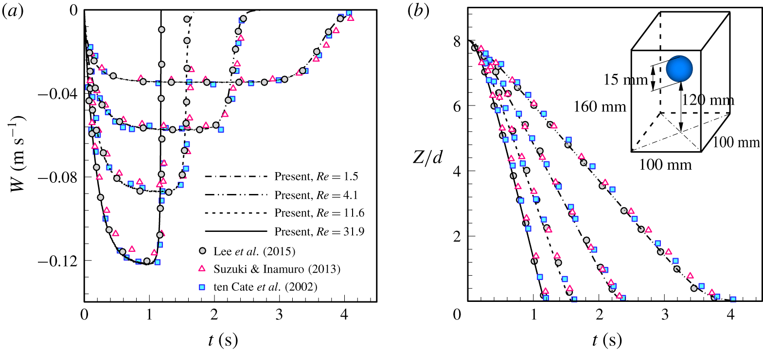
Our computational code was validated by two benchmark tests. The first is the sedimentation of a sphere in a closed box, which has been studied by ten Cate, Nieuwstad & Derksen (Reference ten Cate, Nieuwstad, Derksen and Van den Akker2002) using particle image velocimetry (PIV). The parameters were chosen according to the literature (ten Cate et al. Reference ten Cate, Nieuwstad, Derksen and Van den Akker2002). The diameter of the sphere is  $d=15~\text{mm}$ and its density is fixed at
 $\unicode[STIX]{x1D70C}_{s}=1120~\text{kg}~\text{m}^{-3}$. The box dimensions are
 $\text{depth}\times \text{width}\times \text{height}=100~\text{mm}\times 100~\text{mm}\times 160~\text{mm}$. The sphere is released at a height of 120 mm from the bottom wall. To vary the Reynolds number, four kinds of fluid were considered, as listed in table 1, which also includes the corresponding numerical set-up. For simplicity, the no-slip condition was applied to all boundaries of the box. Figure 2 presents the time history of the sedimentation velocity,
 $W$, as well as the trajectory
 $Z$ of the sphere for all cases considered. The time history agrees well with results from previous PIV (ten Cate et al. Reference ten Cate, Nieuwstad, Derksen and Van den Akker2002), the conventional immersed boundary LBM (Suzuki & Inamuro Reference Suzuki and Inamuro2013) and the extrapolation-based boundary LBM (Lee, Huang & Chiew Reference Lee, Huang and Chiew2015). In these simulations the resolution was fixed at
 $\unicode[STIX]{x0394}x=d/15$, which is identical to that used by Lee et al. (Reference Lee, Huang and Chiew2015). A finer grid resolution (
 $\unicode[STIX]{x0394}x=d/30$) was used by Suzuki & Inamuro (Reference Suzuki and Inamuro2013).
Fluid properties used by ten Cate et al. (Reference ten Cate, Nieuwstad, Derksen and Van den Akker2002) and numerical set-up in our simulations. Note that  $U_{\infty }$ is the settling velocity of a sphere in an infinite domain.

Comparison of our LBM results for  $\unicode[STIX]{x0394}x=d/15$ (lines) with experimental results (squares) (ten Cate et al. Reference ten Cate, Nieuwstad, Derksen and Van den Akker2002), immersed boundary LBM results for
 $\unicode[STIX]{x0394}x=d/30$ (triangles) (Suzuki & Inamuro Reference Suzuki and Inamuro2013) and extrapolation-based boundary LBM results for
 $\unicode[STIX]{x0394}x=d/15$ (circles) (Lee et al. Reference Lee, Huang and Chiew2015) for (a) the settling velocity of the sphere and (b) the trajectory of the sphere.

3.2 Sedimentation of two spheres in a box
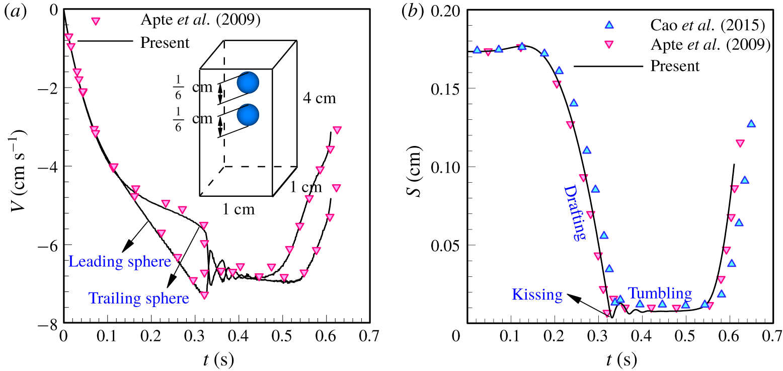
The sedimentation of two identical spheres was simulated to further validate our code in dealing with the hydrodynamic interaction between particles. Numerical calculations were carried out under the same physical conditions as the ones used by Apte, Martin & Patankar (Reference Apte, Martin and Patankar2009). A box with dimensions of  $\text{depth}\times \text{width}\times \text{height}=1~\text{cm}\times 1~\text{cm}\times 4~\text{cm}$ was taken as the computational domain. Two spheres of diameter
 $d=1/6~\text{cm}$ and density
 $\unicode[STIX]{x1D70C}_{s}=1.14~\text{g}~\text{cm}^{-3}$ are initially aligned the vertical direction with their centres
 $2.04d$ apart. The leading sphere is located at (0.5 cm, 0.5 cm, 3.16 cm) and the trailing one is located at (0.5 cm, 0.5 cm, 3.5 cm). The fluid density and dynamic viscosity are
 $\unicode[STIX]{x1D70C}=1~\text{g}~\text{cm}^{-3}$ and
 $\unicode[STIX]{x1D707}=0.01~\text{g}~\text{cm}^{-1}~\text{s}$, respectively. As in the literature (Apte et al. Reference Apte, Martin and Patankar2009; Cao et al. Reference Cao, Chen, Li, Liu, Zha, Bao and Zheng2015), we adopted the repulsive force model proposed by Glowinski et al. (Reference Glowinski, Pan, Hesla, Joseph and Périaux2001) to treat the contact of spheres in this test. The collision parameters (i.e. the cutoff distance, force scale and stiffness parameter) were chosen to be the same as those in Apte et al. (Reference Apte, Martin and Patankar2009). Figure 3(a,b) shows the settling velocity of each sphere and the separation distance between them, respectively, which indicate that a classical DKT motion is reproduced. Moreover, the comparison shows a good agreement with previous numerical results obtained from the finite volume method (Apte et al. Reference Apte, Martin and Patankar2009) and the external-boundary-force-based LBM (Cao et al. Reference Cao, Chen, Li, Liu, Zha, Bao and Zheng2015). Note that Cao et al. (Reference Cao, Chen, Li, Liu, Zha, Bao and Zheng2015) used a larger box with dimensions of
 $1~\text{cm}\times 1~\text{cm}\times 5~\text{cm}$ and different collision parameters in the simulations.
Comparison of our LBM results for  $\unicode[STIX]{x0394}x=d/16$ (solid lines) with previous finite-volume method results for
 $\unicode[STIX]{x0394}x\approx d/13.3$ (gradients) (Apte et al. Reference Apte, Martin and Patankar2009) and external-boundary-force-based LBM results for
 $\unicode[STIX]{x0394}x=d/16$ (triangles) (Cao et al. Reference Cao, Chen, Li, Liu, Zha, Bao and Zheng2015): (a) the settling velocity of each sphere and (b) the separation distance between spheres.

4 Results and discussion
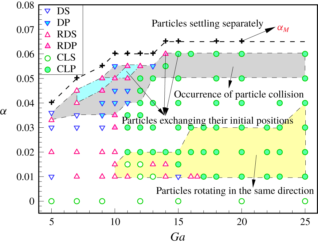
We simulated two spheres of different densities settling in a square tube using a 3-D LBM at low Reynolds numbers. Figure 4 provides an overview of the motion of the spheres for the problem illustrated in figure 1, which summarises the final state of the spheres for  $5\leqslant Ga\leqslant 25$ and
 $0\leqslant \unicode[STIX]{x1D6FC}<\unicode[STIX]{x1D6FC}_{M}$. Note that
 $\unicode[STIX]{x1D6FC}_{M}$ represents the maximum value of
 $\unicode[STIX]{x1D6FC}$ beyond which the heavy sphere leaves the light one behind and they settle separately. According to the final state of particle motion, six sedimentation patterns are identified depending on both Ga and
 $\unicode[STIX]{x1D6FC}$, as shown in figure 4, namely the steady state (DS) and periodic state (DP) in the diagonal plane (i.e.
 $y=x$), the steady state (RDS) and periodic state (RDP) in the reverse–diagonal plane (i.e.
 $y=-x$) and the steady state (CLS) and periodic state (CLP) in the centreline plane (i.e.
 $y=0$).
Final state of the spheres as a function of Ga ( $5\leqslant Ga\leqslant 25$) and
 $\unicode[STIX]{x1D6FC}$ (
 $0\leqslant \unicode[STIX]{x1D6FC}<\unicode[STIX]{x1D6FC}_{M}$), where
 $\unicode[STIX]{x1D6FC}_{M}$ represents the maximum of
 $\unicode[STIX]{x1D6FC}$ beyond which the two spheres begin to settle separately in the tube. According to the final state of particle motion, six sedimentation patterns are identified. DS: steady state in the diagonal plane (i.e.
 $y=x$); DP: periodic state in the diagonal plane (i.e.
 $y=x$); RDS: steady state in the reverse–diagonal plane (i.e.
 $y=-x$); RDP: periodic state in the reverse–diagonal plane (i.e.
 $y=-x$); CLS: steady state in the centreline plane (i.e.
 $y=0$); CLP: periodic state in the centreline plane (i.e.
 $y=0$).

For  $\unicode[STIX]{x1D6FC}=0$, the case of equal particles, the two spheres always reach a steady state in the centreline plane (CLS) where they are released from rest. The situation becomes quite different for unequal spheres. For
 $\unicode[STIX]{x1D6FC}\geqslant 0.02$ the spheres eventually move to the diagonal or reverse–diagonal plane of the tube when Ga is below a certain value. The CLP pattern appears at high Ga. By contrast, it is difficult to find the CLS pattern for unequal spheres (except for
 $\unicode[STIX]{x1D6FC}=0.01$ at
 $Ga=12$ and 13, and
 $\unicode[STIX]{x1D6FC}=0.015$ at
 $Ga=11$ and 12), as shown in figure 4. Furthermore, the steady state of the spheres may bifurcate into periodic motion when either Ga or
 $\unicode[STIX]{x1D6FC}$ increases, which, however, has different effects on the motion of the spheres. This will be presented later. The motions of spheres in the (reverse–) diagonal plane and the centreline plane are discussed in §§ 4.1 and 4.2, respectively.
4.1 Particle motion in the (reverse–) diagonal plane of the tube
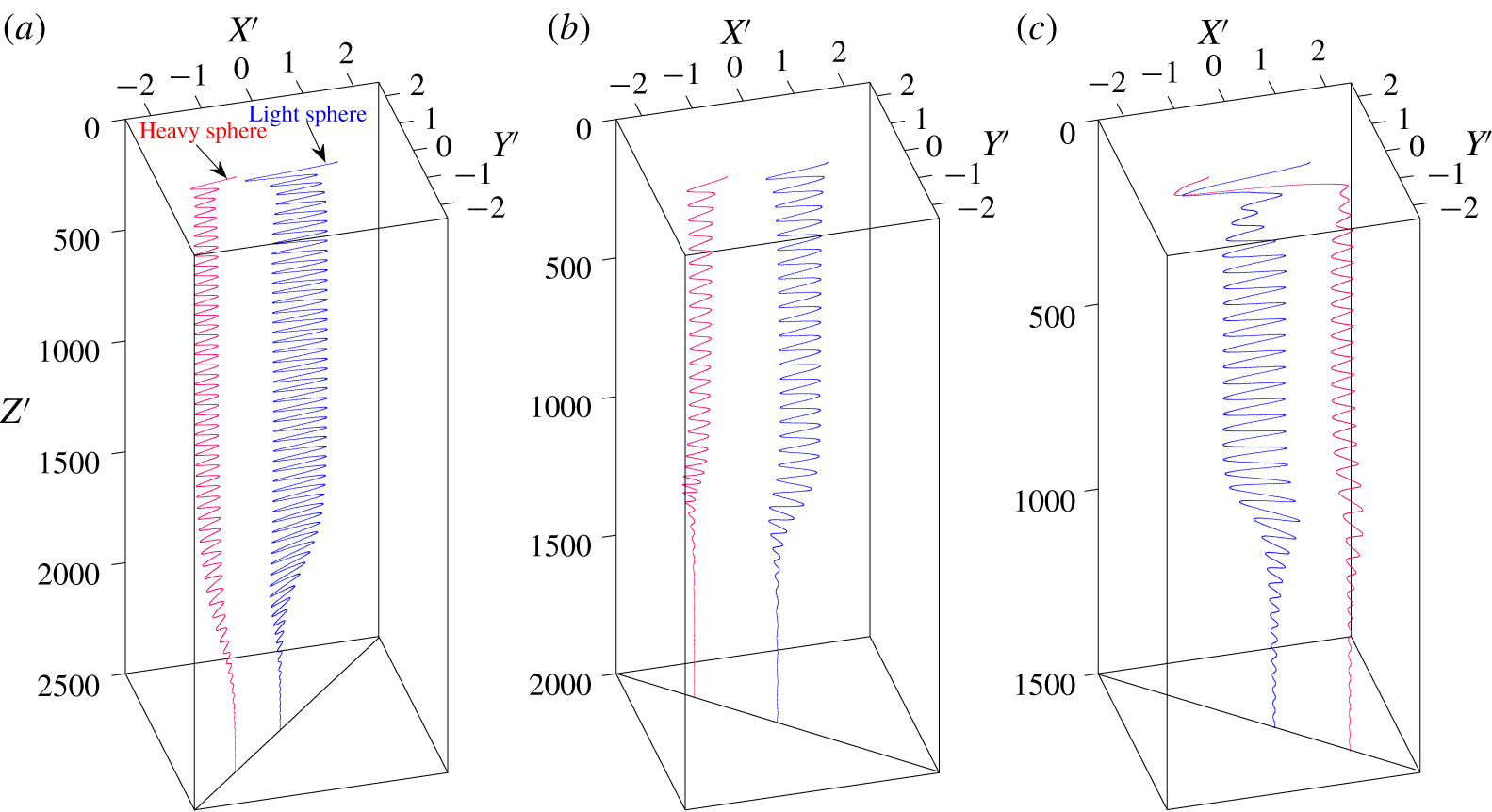
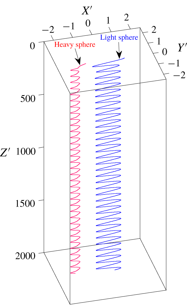
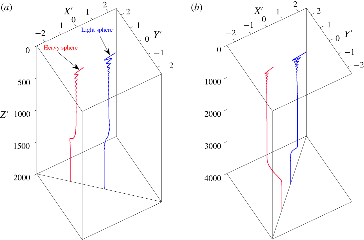
Figure 5(a) shows the trajectories of both spheres for  $\unicode[STIX]{x1D6FC}=0.03$ at
 $Ga=5$, representing the DS pattern. For better illustration, the particle positions are normalised by:
 $X^{\prime }(t)=X(t)/d,Y^{\prime }(t)=Y(t)/d$ and
 $Z^{\prime }(t)=[Z(0)-Z(t)]/d$. It has been shown that the spheres periodically oscillate in the centreline plane of the tube as they settle for a time (
 $Z_{1}^{\prime }\leqslant 1000$). The oscillation amplitude is seen to be much larger for the light sphere. Then both spheres begin to leave the centreline plane. It takes a very long time for them to move to the diagonal plane of the tube (i.e.
 $y=x$). During this process the oscillations of both spheres gradually attenuate because of the increasing domain of the plane, and a steady state is eventually reached, as shown in figure 5(a).
Trajectories of the spheres for different settings: (a)  $\unicode[STIX]{x1D6FC}=0.03$ at
 $Ga=5$ (DS pattern), (b)
 $\unicode[STIX]{x1D6FC}=0.02$ at
 $Ga=7$ (RDS pattern) and (c)
 $\unicode[STIX]{x1D6FC}=0.04$ at
 $Ga=7$ (RDS pattern with particles exchanging initial positions). For better illustration, the positions of the spheres are normalised by:
 $X^{\prime }(t)=X(t)/d,Y^{\prime }(t)=Y(t)/d,Z^{\prime }(t)=[Z(0)-Z(t)]/d$. The same as below.

The spheres may move to the reverse–diagonal plane of the tube at low Galileo numbers, as illustrated in figure 4. Figure 5(b) shows the trajectories of both spheres for  $\unicode[STIX]{x1D6FC}=0.02$ at
 $Ga=7$, which exhibits the pattern of RDS. Similar behaviour is observed except that the spheres eventually reach stable positions in the reverse–diagonal plane (i.e.
 $y=-x$). Moreover, we find that increasing the density difference
 $\unicode[STIX]{x1D6FC}$ may cause the particles to exchange positions, as seen in figure 5(c), which presents the corresponding results for
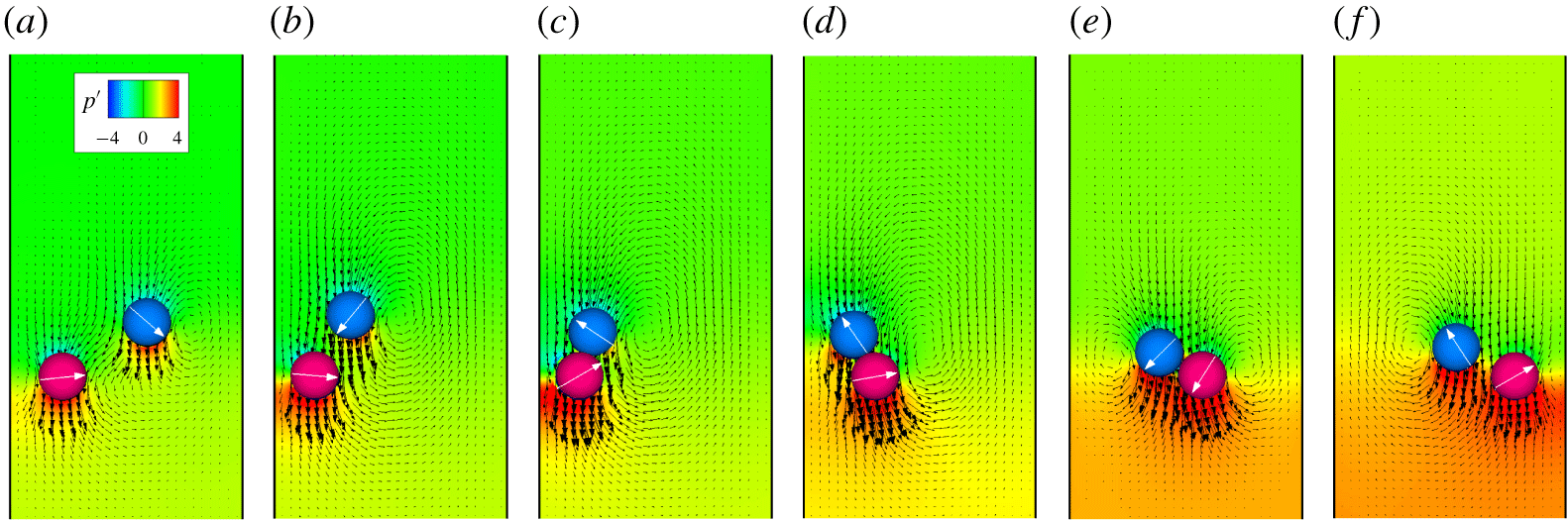
 $\unicode[STIX]{x1D6FC}=0.04$ at the same Ga as that of figure 5(b). To better address this issue, a series of flow fields are illustrated in figure 6, showing the interactions between the two spheres during the early settling stage.
After the spheres are released from a horizontal line, the heavy sphere settles quickly near a wall owing to its large density. Soon the light sphere is sucked into the wake of the heavy one and drafts toward it with increasing velocity (figures 6a and 6b). Then, the particles come into contact (figures 6c and 6d). However, the structure in which the spheres are standing vertically is unstable. The strong wall repulsion drives the heavy sphere away from the nearby wall, and the light sphere moves around the heavy one at the same time. This behaviour is similar to the well-known DKT pattern reported early by Fortes et al. (Reference Fortes, Joseph and Lundgren1987) and Feng et al. (Reference Feng, Hu and Joseph1994). However, the spheres do not tumble because the bottom sphere is heavier. Due to the strong interparticle repulsion they begin to separate (figures 6e and 6f). As shown in figure 4, the exchange of particle positions only occurs at high  $\unicode[STIX]{x1D6FC}$ for
 $7\leqslant Ga\leqslant 15$. This can be interpreted as follows. On the one hand, large
 $\unicode[STIX]{x1D6FC}$ is needed for the heavy sphere to produce a strong downward stream to quickly attract the light sphere into the wake. This results in a configuration in which the two spheres are in contact with the light one directly above the heavy one. On the other hand, because of the high pressure between the heavy sphere and the nearby wall, the heavy sphere is ejected with a large lateral velocity to the centreline. As a result, the light sphere moves counter-clockwise around the heavy one and eventually stays on its left side. As Ga increases, the pressure between the heavy sphere and the wall becomes insignificant, which will be shown below. This is why the particles do not exchange positions at
 $Ga\geqslant 16$.
Instantaneous flow fields in the centreline plane at different times for  $\unicode[STIX]{x1D6FC}=0.04$ at
 $Ga=7$: (a)
 $t^{\prime }=55.3$, (b)
 $t^{\prime }=110.7$, (c)
 $t^{\prime }=138.4$, (d)
 $t^{\prime }=166$, (e)
 $t^{\prime }=193.7$ and (f)
 $t^{\prime }=248.9$. The pressure is normalised through
 $p^{\prime }=(p-p_{\infty })/(\unicode[STIX]{x1D70C}U_{T}^{2})$. The value of
 $p_{\infty }$ represents the pressure of the undisturbed flow. The time is normalised through
 $t^{\prime }=t/T_{0}$. The arrow on each particle represents its orientation with respect to the horizontal direction, which is zero when the particle is released.

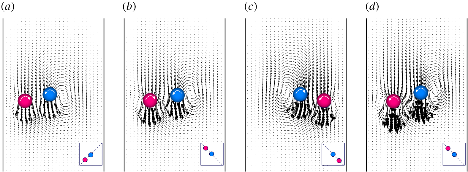
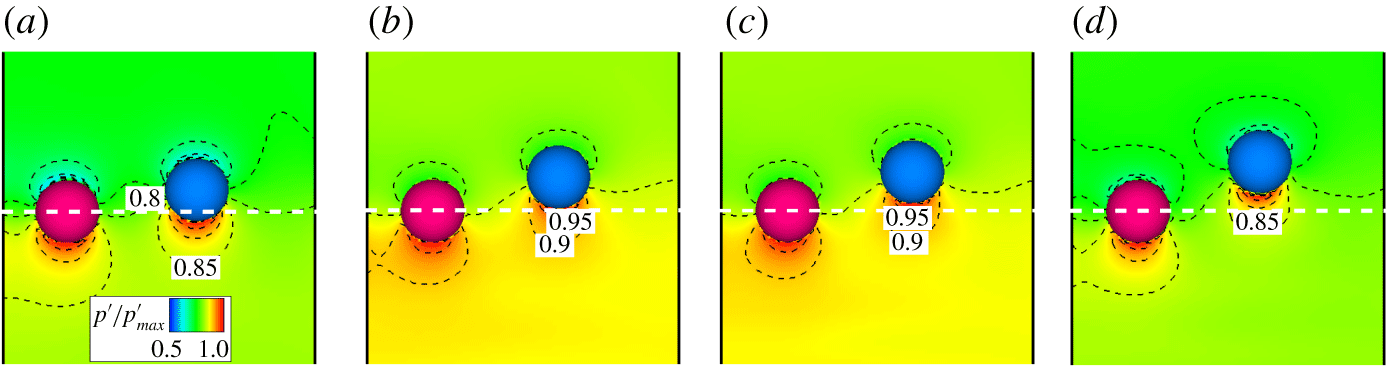
Figure 4 shows a strong tendency for the spheres to find stable positions in the diagonal or reverse–diagonal plane at low Galileo numbers when the spheres are not identical (i.e.  $\unicode[STIX]{x1D6FC}>0$). To shed light on this, figure 7 shows the instantaneous flow fields in the diagonal plane (DS) or reverse–diagonal plane (RDS) at the steady state for some sample settlings. All the results exhibit a stable staggered structure similar to that seen in the two-dimensional analysis (Nie et al. Reference Nie, Lin and Gao2017; Nie & Lin Reference Nie and Lin2019). However, there are still two significant differences between the 2-D and 3-D computations. First, two recirculation zones rotating in opposite directions form on the opposite side of each sphere. However, these zones rotate in the same direction and appear on the same side of each circular cylinder at similar Reynolds numbers. Second, the heavy particle rotates in the same direction as the light one for the 2-D computations at low Ga. This is known as ‘abnormal rotation’ because it seems as though the heavy particle rolls up the wall when it is settling in the channel. In contrast, abnormal rotation only occurs when
 $Ga\geqslant 10$ for the 3-D case (figure 4). In addition, both figures 5 and 6 show that at the steady state the light sphere always stays in a position which is close to the tube axis while the heavy one is close to the walls. The reason why the spheres move to the (reverse–) diagonal plane of the tube will be discussed in § 4.3.
Staggered structures (velocity fields) in the diagonal plane ( $y=x$) or reverse–diagonal plane (
 $y=-x$) at the steady state for (a)
 $Ga=5$ and
 $\unicode[STIX]{x1D6FC}=0.03$ (DS), (b)
 $Ga=7$ and
 $\unicode[STIX]{x1D6FC}=0.01$ (RDS), (c)
 $Ga=7$ and
 $\unicode[STIX]{x1D6FC}=0.04$ (RDS with particles exchanging initial positions) and (d)
 $Ga=10$ and
 $\unicode[STIX]{x1D6FC}=0.01$ (RDS with ‘abnormal rotation’ of the heavy sphere).

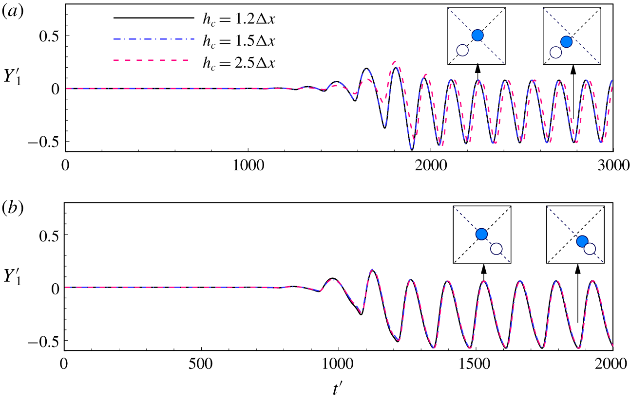
Figure 4 also shows that for large  $\unicode[STIX]{x1D6FC}$ the spheres oscillate in the (reverse–) diagonal plane of the tube when Ga is low. Figure 8(a) and 8(b) show the lateral position of the light sphere (
 $Y_{1}^{\prime }$) for DP and RDP patterns, respectively. We remark that the particles may collide when
 $\unicode[STIX]{x1D6FC}$ is large owing to the significant particle inertia. To check the effect of the collision (2.7) on the particle motion, the cutoff distance (i.e. the value of
 $h_{c}$) is varied. The comparison is also made in figure 8. We see that the trajectories are not sensitive to
 $h_{c}$, although there is a very small discrepancy between these results with
 $h_{c}=1.2\unicode[STIX]{x0394}x$ and those obtained using
 $h_{c}=2.5\unicode[STIX]{x0394}x$. We infer that collision does not affect the motion pattern of the spheres by considering that the cutoff distance is usually of the order of one lattice spacing.
Time history of the lateral position of the light sphere,  $Y_{1}^{\prime }$, for (a)
 $Ga=10$ and
 $\unicode[STIX]{x1D6FC}=0.04$ (DP) and (b)
 $Ga=12$ and
 $\unicode[STIX]{x1D6FC}=0.055$ (RDP). The collision model (2.7) was also examined by varying the value of
 $h_{c}$ (cutoff distance).

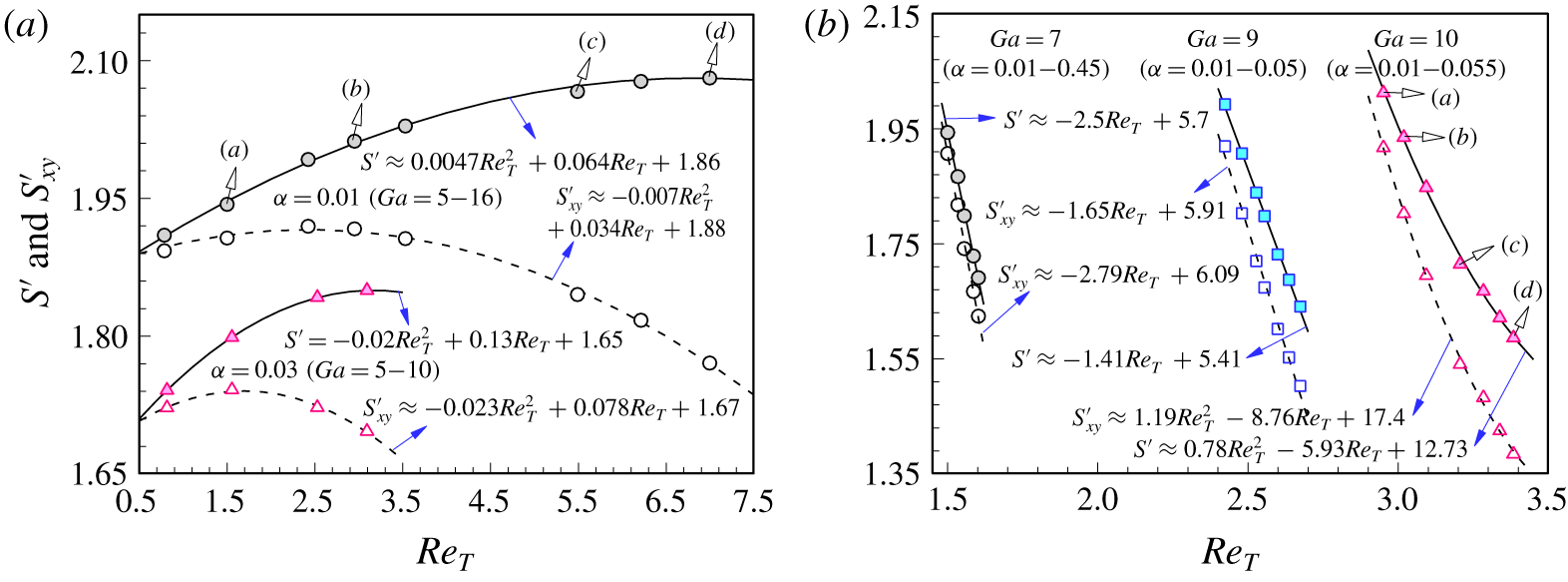
To gain further insight into particle motion in the (reverse–) diagonal plane, we show the effects of  $Re_{T}$ on the normalised distance between spheres,
 $S^{\prime }$, in figure 9 along with its projection onto the xoy plane,
 $S_{xy}^{\prime }$. The average values of
 $S^{\prime }$ and
 $S_{xy}^{\prime }$ are used for the periodic state of the spheres. Note that
 $Re_{T}$ is varied in two ways: increasing Ga when
 $\unicode[STIX]{x1D6FC}$ is fixed (figure 9a) or increasing
 $\unicode[STIX]{x1D6FC}$ when Ga is fixed (figure 9b). A quadratic relationship between
 $S^{\prime }$ or
 $S_{xy}^{\prime }$ and
 $Re_{T}$ is clear in figure 9(a). The distance between the heavy and light spheres increases with the Reynolds number, owed primarily to the increasing effect of the wake. In contrast, figure 9(b) shows an opposite effect of
 $Re_{T}$ on
 $S^{\prime }$ when
 $\unicode[STIX]{x1D6FC}$ increases at fixed Ga. Both
 $S^{\prime }$ and
 $S_{xy}^{\prime }$ decrease rapidly with increasing
 $Re_{T}$ in all three cases (
 $Ga=7,9$ and 10). Figure 9(b) also shows a nearly linear relationship between
 $S^{\prime }$ or
 $S_{xy}^{\prime }$ and
 $Re_{T}$ for
 $Ga=7$ and 9 owing to the weak effect of fluid inertia at very low Reynolds numbers. The relationship becomes quadratic for
 $Ga=10$. The main reason for the difference between figures 9(a) and 9(b) is the effect of particle–wall interactions, which is illustrated in figures 10 and 11.
Distance between particle centres,  $S^{\prime }$ (filled symbols), and projection of
 $S^{\prime }$ onto the xoy plane,
 $S_{xy}^{\prime }$ (open symbols), versus Reynolds number
 $Re_{T}$ with increasing (a) Ga and (b)
 $\unicode[STIX]{x1D6FC}$. Note that
 $S^{\prime }=S/d$ and
 $S_{xy}^{\prime }=S_{xy}/d$. Also shown is the fitting curve for each result. Curves (a–d) in panel (a) correspond to the Ga values in figure 10(a–d), respectively, and curves (a–d) in panel (b) correspond to the
 $\unicode[STIX]{x1D6FC}$ values in figure 11(a–d), respectively.

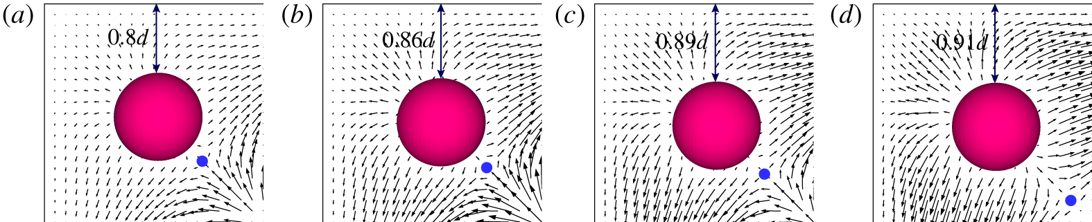
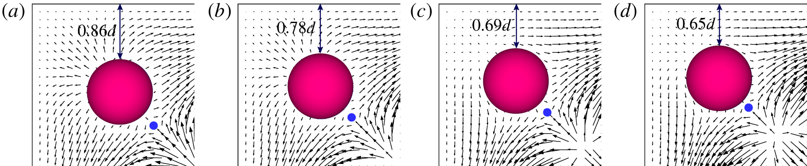
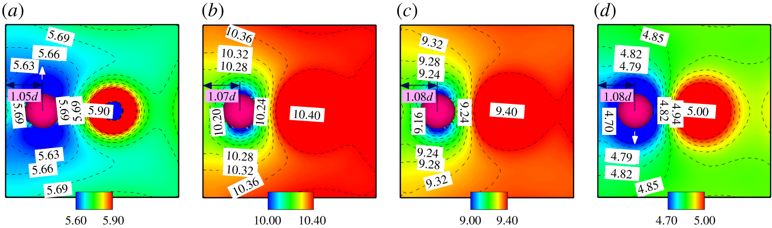
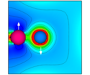
Figure 10 shows the transverse flow fields (top view) around the heavy sphere for  $\unicode[STIX]{x1D6FC}=0.01$ at different values of Ga (note that the two spheres have different vertical positions). The distance between the heavy sphere and nearby wall increases monotonically as Ga increases. However, this distance behaves oppositely with increasing
 $\unicode[STIX]{x1D6FC}$ in figure 11. The blocking becomes more significant as the heavy sphere comes closer to the walls, which suppresses the magnitude and range of its wake. As a consequence, the light sphere comes nearer to the heavy one for larger
 $\unicode[STIX]{x1D6FC}$ when Ga is constant. Furthermore, figures 10 and 11 reveal a stagnation point (blue circle in each panel) in the plane of the heavy sphere, which results from the meeting of two outward streams in the diagonal of this plane. There is no stagnation point in the plane of the light sphere because there is one outward stream and one inward stream.
Transverse flow fields (top view) around the heavy sphere for  $\unicode[STIX]{x1D6FC}=0.01$ at (a)
 $Ga=7$, (b)
 $Ga=10$, (c)
 $Ga=14$ and (d)
 $Ga=16$ (corresponding to curves (a–d) in figure 9(a), respectively). The blue circles represent stagnation points in the flow fields.

Transverse flow fields (top view) around the heavy sphere at  $Ga=10$ for (a)
 $\unicode[STIX]{x1D6FC}=0.01$, (b)
 $\unicode[STIX]{x1D6FC}=0.02$, (c)
 $\unicode[STIX]{x1D6FC}=0.04$ and (d)
 $\unicode[STIX]{x1D6FC}=0.055$ (corresponding to curves (a–d) in figure 9(b), respectively). Note that the flow fields for
 $\unicode[STIX]{x1D6FC}=0.04$ and
 $\unicode[STIX]{x1D6FC}=0.055$, which correspond to the DS pattern, are rotated clockwise by 90 degrees for direct comparison.

4.2 Particle motion in the centreline plane of the tube
As shown in figure 4, the two spheres are likely to exhibit periodic motion in the centreline plane of the tube at high Galileo numbers when  $\unicode[STIX]{x1D6FC}>0$. Figure 12 shows the trajectories of the spheres for
 $\unicode[STIX]{x1D6FC}=0.03$ at
 $Ga=11$, representing the pattern of CLP. Numerical results show that the spheres never leave the plane where they are released from rest. To better illustrate the CLP pattern, we present the limit cycle constructed with
 $X_{1}^{\prime }$ and
 $X_{2}^{\prime }$ for each
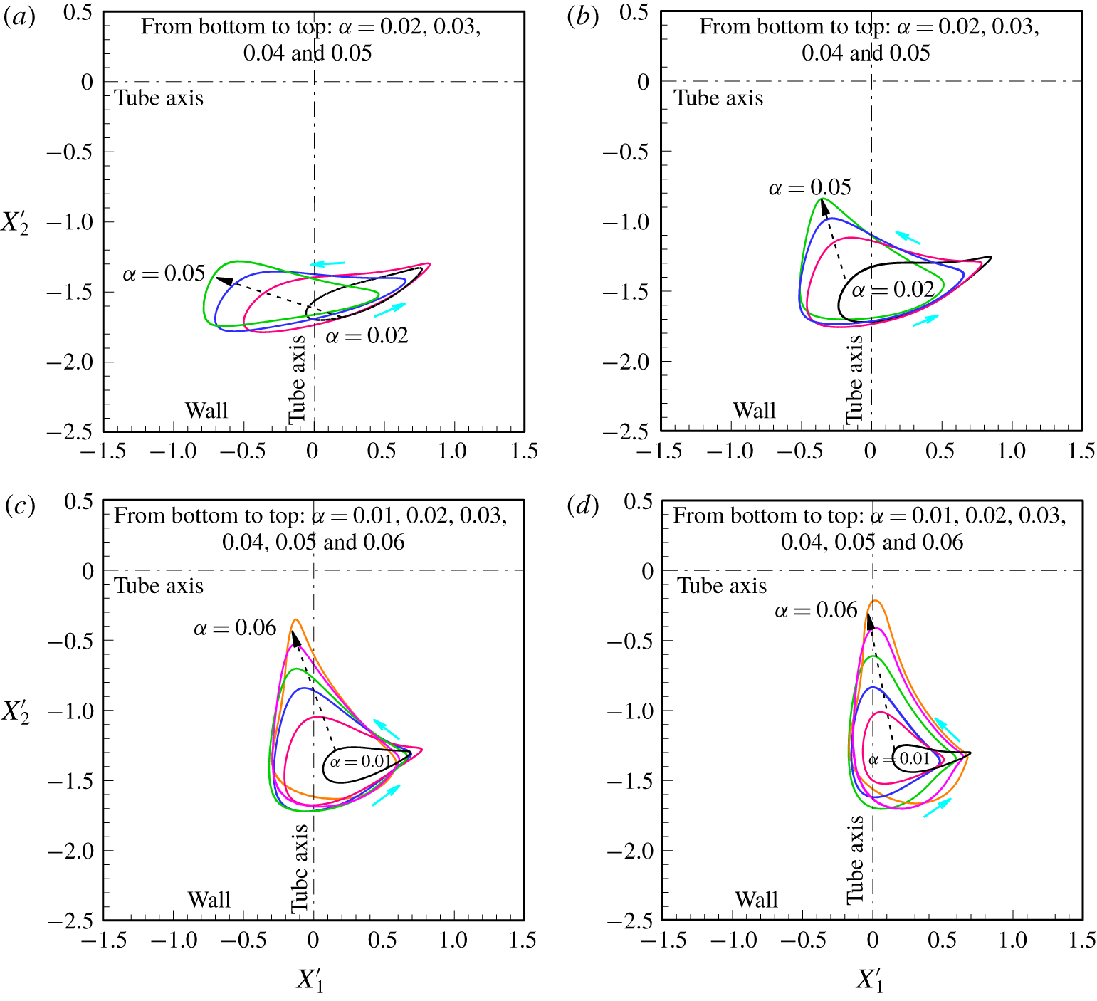
 $\unicode[STIX]{x1D6FC}$ at four sample Ga values (12, 15, 20 and 25) in figure 13.
Trajectories of the spheres for  $\unicode[STIX]{x1D6FC}=0.03$ at
 $Ga=11$ (CLP).

For fixed Ga, increasing  $\unicode[STIX]{x1D6FC}$ always leads to a larger limit cycle. On the one hand, the oscillation amplitude is larger for the light sphere regardless of
 $\unicode[STIX]{x1D6FC}$ at low Ga (figure 13a), which agrees with figure 12. On the other hand, the amplitude of
 $X_{2}^{\prime }$ increases more significantly at high Ga (figures 13c and 13d). At
 $Ga=25$, for instance, the amplitude of
 $X_{1}^{\prime }$ is nearly triple that for
 $\unicode[STIX]{x1D6FC}=0.01$. However, the amplitude of
 $X_{1}^{\prime }$ becomes nearly half that of
 $X_{2}^{\prime }$ for
 $\unicode[STIX]{x1D6FC}=0.06$. This implies that at higher Reynolds numbers the inertia of solid particles becomes strong and makes the periodic motion more sensitive to
 $\unicode[STIX]{x1D6FC}$. In most cases in figure 13 the light sphere oscillates around the axis of the tube, while the heavy sphere always oscillates around a line between the tube axis and nearby wall.
Limit cycles for different values of  $\unicode[STIX]{x1D6FC}$ at (a)
 $Ga=12$, (b)
 $Ga=15$, (c)
 $Ga=20$ and (d)
 $Ga=25$.

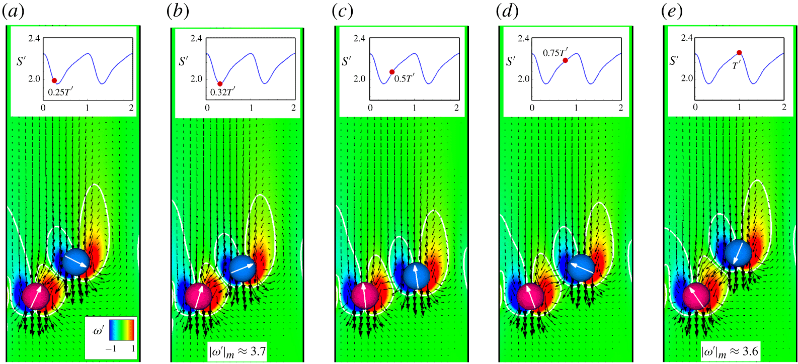
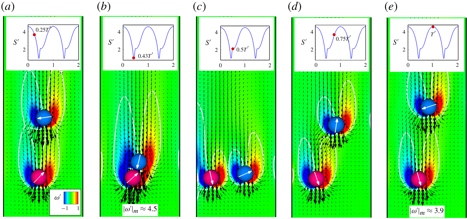
Figures 14 and 15 show the instantaneous velocity fields and vorticity contours at different times during one oscillation period for  $\unicode[STIX]{x1D6FC}=0.01$ (
 $T^{\prime }\approx 304.9$) and
 $\unicode[STIX]{x1D6FC}=0.06(T^{\prime }\approx 228.4)$, respectively, at
 $Ga=25$. These figures illustrate the interactions between the spheres as they oscillate with very different intensities and show the variation in distance between them. In figures 14 and 15, it is always the wake suction that causes a persistent oscillation in the motion and rotation of the spheres, with the amplitude and frequency depending on
 $\unicode[STIX]{x1D6FC}$. Compared with
 $\unicode[STIX]{x1D6FC}=0.01$, the wake of the heavy sphere drags the light sphere much closer to it for
 $\unicode[STIX]{x1D6FC}=0.06$ owing to more significant fluid inertia (note the vorticity maximum indicated in figures 14b and 15b). Meanwhile, for
 $\unicode[STIX]{x1D6FC}=0.06$ the light sphere is thrown out of the wake farther away from the heavy sphere when they get close enough (figures 14e and 15e). In addition, the particle oscillation is much faster for
 $\unicode[STIX]{x1D6FC}=0.06$ than for
 $\unicode[STIX]{x1D6FC}=0.01$ (note the period). Another significant difference in flow features is that two recirculation zones rotating in opposite directions are generated between the spheres at
 $t^{\prime }=0.5T^{\prime }$ for
 $\unicode[STIX]{x1D6FC}=0.06$ (figure 15c), which is not the case for
 $\unicode[STIX]{x1D6FC}=0.01$. This is also a consequence of strong fluid inertia.
Instantaneous velocity fields and vorticity contours ( $\unicode[STIX]{x1D714}^{\prime }=\unicode[STIX]{x1D714}d/U_{0}$) in the centreline plane during one period (
 $T^{\prime }\approx 304.9$) for
 $\unicode[STIX]{x1D6FC}=0.01$ at
 $Ga=25$: (a)
 $0.25T^{\prime }$, (b)
 $0.32T^{\prime }$, (c)
 $0.5T^{\prime }$, (d)
 $0.75T^{\prime }$ and (e)
 $T^{\prime }$. The distance between spheres,
 $S^{\prime }$, at the time is indicated in each panel. The vorticity contours for
 $|\unicode[STIX]{x1D714}^{\prime }|=0.2$ are also identified in each panel. The vorticity maximum
 $|\unicode[STIX]{x1D714}^{\prime }|_{m}$ is presented in (b,e), corresponding to the times when
 $S^{\prime }$ reaches its minimum and maximum, respectively.

Instantaneous velocity fields and vorticity contours in the centreline plane during one period ( $T^{\prime }\approx 228.4$) for
 $\unicode[STIX]{x1D6FC}=0.06$ at
 $Ga=25$: (a)
 $0.25T^{\prime }$, (b)
 $0.43T^{\prime }$, (c)
 $0.5T^{\prime }$, (d)
 $0.75T^{\prime }$ and (e)
 $T^{\prime }$. The vorticity maximum
 $|\unicode[STIX]{x1D714}^{\prime }|_{m}$ is presented in (b,e), corresponding to the times when
 $S^{\prime }$ reaches its minimum and maximum, respectively.

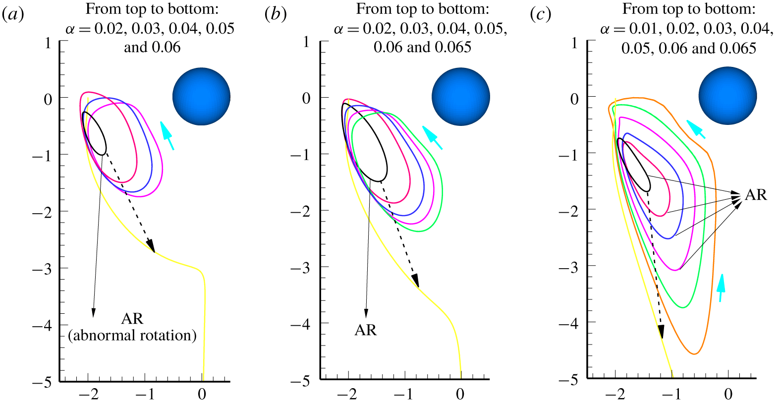
The relative particle trajectories may better illustrate the periodic motion of the interacting spheres and are shown in figure 16 for  $Ga=12$, 15 and 25. Note that these relative trajectories are obtained under the condition that the light sphere is fixed. For each value of
 $\unicode[STIX]{x1D6FC}$ the relative particle trajectory is a closed orbit when
 $\unicode[STIX]{x1D6FC}<\unicode[STIX]{x1D6FC}_{M}$. As expected, the size of the orbit increases as
 $\unicode[STIX]{x1D6FC}$ increases for each Ga. As shown in figure 4, the heavy sphere rotates in the same direction as the light one when
 $\unicode[STIX]{x1D6FC}$ is small, while the opposite is true when
 $\unicode[STIX]{x1D6FC}$ is large. In particular, the change in rotation sign of the heavy sphere causes a sudden enlargement of the closed orbits for low Ga (figure 16a). This sudden jump becomes insignificant as Ga is gradually increased (figure 16b,c). Periodic motion of two unequal spheres settling in a viscous fluid was studied as early as the 1970s by Wacholder & Sather (Reference Wacholder and Sather1974), who obtained the relative particle trajectories by solving the Stokes equations. In their study, two spheres with different sizes and densities move freely under the action of gravity in an unconfined quiescent fluid. For certain conditions, Wacholder & Sather (Reference Wacholder and Sather1974) predicted that the larger sphere would oscillate around the smaller one if their initial distance was below a critical value. This is qualitatively consistent with our results.
Relative trajectories of the spheres when the light sphere is fixed at (a)  $Ga=12$, (b)
 $Ga=15$ and (c)
 $Ga=25$.

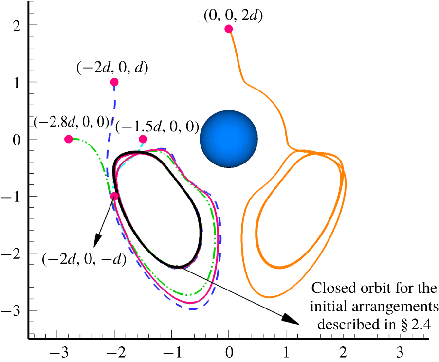
At the end of this section, an examination of the initial arrangements on the motion of spheres for  $\unicode[STIX]{x1D6FC}=0.05$ at
 $Ga=15$ is presented. In doing so the initial position of the heavy sphere is varied while the initial position of the light one is kept unchanged. Five sets of initial arrangements are taken into account. Note that the initial positions of the heavy sphere indicated in figure 17 are relative to that of the light one. As shown in figure 17, after the initial transients die down all the relative trajectories achieve the same limit cycle as the one obtained from the initial arrangements described in § 2.4 except for the result of (0, 0, 2d), which exhibits a different but symmetric limit cycle, instead. However, it can be still inferred that all the initial arrangements considered predict the same periodic motion of spheres in terms of the amplitude and frequency of the oscillations. Therefore, it may be concluded that the patterns shown in figure 4 hold for a variety of initial arrangements of the two spheres.
Examination of the initial arrangements on the motion of spheres for  $\unicode[STIX]{x1D6FC}=0.05$ at
 $Ga=15$. Different initial positions of the heavy sphere (relative to the light sphere) are also indicated in the figure. All results are compared with the closed orbit of relative trajectory obtained from the initial arrangements described in § 2.4.

4.3 Possible mechanism
In this section we discuss the possible mechanism for the movement of the spheres to the (reverse–) diagonal plane under certain conditions. Figure 4 shows that two unequal particles ( $\unicode[STIX]{x1D6FC}>0$) may leave the centreline plane where they are initially released from rest at low Galileo numbers. Furthermore, the steady state of the two spheres is usually achieved in the (reverse–) diagonal plane over the whole ranges of Ga and
 $\unicode[STIX]{x1D6FC}$ studied (except for
 $\unicode[STIX]{x1D6FC}=0$), which implies that generally the spheres stay in periodic motion in the centreline plane (CLP). For the problem illustrated in figure 1, the spheres settle in the tube under the combined effects of gravity and fluid viscosity, and hence the interplay between these two factors determines the pattern of this sedimentation system. We may roughly conclude from figure 4 that the spheres stay in the centreline plane owing to the significant effect of gravity. This is why the diagonal motion patterns (DS, DP, RDS and RDP) are not observed at high Ga. However, this needs further study.
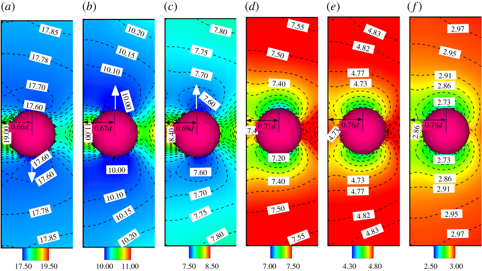
Instantaneous pressure distributions (top view) around the heavy sphere when it is closest to the nearby wall for  $\unicode[STIX]{x1D6FC}=0.03$ at (a)
 $Ga=5$ (DS), (b)
 $Ga=7$ (RDS), (c)
 $Ga=9$ (RDS), (d)
 $Ga=12$ (CLP), (e)
 $Ga=17$ (CLP) and (f)
 $Ga=20$ (CLP). Each panel also shows the distance between the heavy sphere and the nearby wall. The white arrow in (a–c) shows the direction of motion of the heavy sphere as it begins to leave the centreline plane.

At low Ga the spheres oscillate in the centreline plane for a long time before they leave (figure 5). Taking  $\unicode[STIX]{x1D6FC}$ = 0.03 for example, figure 18 shows the instantaneous pressure distributions (top view) around the heavy sphere at various Ga values when the heavy sphere comes closest to the nearby wall in the centreline plane. For each Ga, sample
 $p^{\prime }$ values are identified in the figure for better illustration. For low Ga (figure 18a–c) there is a high-pressure zone between the heavy sphere and the nearby wall, which gives rise to a strong repulsive force that pushes the heavy sphere away from the wall. In contrast, a low-pressure zone forms on its upper side and on its lower side, (figure 18a–c). As a result, the heavy sphere has a strong tendency to move into the low-pressure zones when it gains high lateral velocity from the wall repulsion. Movement upwards corresponds to RDS or RDP, while downwards entails DS or DP. The light sphere is accordingly forced to leave the centreline plane because of the hydrodynamic interactions. Therefore, the centreline plane is an unstable place for the spheres when Ga is low. The situation nearly reverses at high Ga (figure 18d–f). High-pressure zones (compared with the pressure between the heavy sphere and nearby wall) are now on the upper and lower sides of the heavy sphere instead (except small areas close to it). This obviously inhibits the heavy sphere from going upwards or downwards in the top view plane, which ensures that the spheres stay in the centreline plane. However, it seems uncertain why the spheres go to the reverse–diagonal plane more likely than the diagonal plane (see figure 4). In other words, we can predict whether or not the spheres stay in the centreline plane where they are initially released. If the spheres do not stay in the centreline plane, however, we are not sure whether they go to the diagonal plane (or reverse–diagonal plane).
Figure 18 also reveals that the heavy sphere is closer to the wall at lower Ga (as in figure 10), resulting in a stronger wall repulsion. This is also responsible for the particle motion in the (reverse–) diagonal plane at low Ga. It is worth remarking here that the wall repulsion also has significant influence on the sedimentation of circular cylinders at low Reynolds numbers. Previous studies (Feng et al. Reference Feng, Hu and Joseph1994; Nie et al. Reference Nie, Lin and Gao2017) show that two circular cylinders which are initially placed symmetrical about the axis of a channel exhibit a stable staggered structure as they are settling in the channel. The initial in-line configuration of particles is eventually ruined by the strong wall repulsion.
Trajectories of the spheres for  $\unicode[STIX]{x1D6FC}=0.01$ at (a)
 $Ga=9$ (RDS) and (b)
 $Ga=15$ (DS), respectively.

As stated before, the CLS pattern does not appear for unequal particles except for  $\unicode[STIX]{x1D6FC}=0.01$ (
 $Ga=12$ and 13) and
 $\unicode[STIX]{x1D6FC}=0.015$ (
 $Ga=11$ and 12), as shown in figure 4. Simulations show that for low
 $\unicode[STIX]{x1D6FC}$ (such as 0.01) the spheres quickly arrive at their stable positions in the centreline plane. Figure 19 presents the trajectories of the spheres for
 $\unicode[STIX]{x1D6FC}=0.01$ at
 $Ga=9$ and
 $Ga=15$, which correspond to the RDS and DS patterns, respectively. Compared with figure 5, figure 19 has a significant difference: the particles remain stable in the centreline plane for some time (
 $Z_{1}^{\prime }\leqslant 750$ for
 $Ga=9$ and
 $Z_{1}^{\prime }\leqslant 2500$ for
 $Ga=15$) before going to the (reverse–) diagonal plane.
Similarly, to examine the motion pattern, we show the instantaneous pressure distributions in the plane of the heavy sphere (top view) for  $\unicode[STIX]{x1D6FC}=0.01$ at
 $Ga=9$, 12, 13 and 15 in figure 20. Each distribution is chosen when the spheres are stable in the centreline plane. For low Ga (figure 20a) the situation is similar to that of figure 18(a–c) in that there is a high-pressure zone between the heavy sphere and nearby wall (compared with the pressure on the lateral sides of the sphere). For higher Ga (figure 20d), however, this high-pressure zone is not seen because the heavy sphere moves farther away from the wall (note the distance indicated in each panel). Instead, the pressure on its right side becomes significant because of the strong hydrodynamic interaction with the light sphere. This gives rise to the DS or RDS pattern. For intermediate Ga (such as 12 or 13) as shown in figure 20(b,c), the situation is somewhat unique because the spheres stay in the centreline plane for a very long time (
 $Z_{1}^{\prime }>10000$). In view of the high-pressure zones on the upper and lower sides of the plane of the heavy sphere (figure 20b,c), we infer that the spheres will never go to the (reverse–) diagonal plane. For this special situation the pressure distributions in the centreline plane (front view) may provide a better understanding, as shown in figure 21. The structure of the spheres is more staggered at higher Ga. In other words, the vertical distance between the spheres increases as Ga increases. The plane of the heavy sphere is exactly located in the highest-pressure zone below the light sphere when
 $Ga=12$ or 13, as illustrated in figure 21(b,c). This results in the unique pressure distributions shown in figure 20(b,c).
Instantaneous pressure distributions (top view) around the heavy sphere for  $\unicode[STIX]{x1D6FC}=0.01$ at (a)
 $Ga=9$ (RDS), (b)
 $Ga=12$ (CLS), (c)
 $Ga=13$ (CLS) and (d)
 $Ga=15$ (RDS). Each distribution is chosen when the spheres are stable in the centreline plane.

Instantaneous pressure distributions in the centreline plane (front view) corresponding to panels (a–d) of figure 20. The dashed line in each figure represents the location of the plane of the heavy sphere.

4.4 Comparison between the 2-D and 3-D computations
In particulate flows, 2-D simulations are usually used to study interactions between spheres at low Reynolds number because the dynamical features of the 2-D and 3-D systems are similar. The problem treated in this study was simulated for the 2-D case in our previous work (Nie et al. Reference Nie, Lin and Gao2017; Nie & Lin Reference Nie and Lin2019), in which two circular cylinders with different densities in a channel exhibited a steady or periodic state depending on both Ga and the density difference between the particles. This qualitatively agrees with its 3-D counterpart. However, the present work shows that the extra dimension allows different patterns of particle behaviour. For instance, it would not be possible to predict the diagonal motion of particles in a 2-D channel at low Ga. In addition, there are two kinds of periodic states for the circular cylinders, characterised by the decay (at low Ga) or growth (at high Ga) of oscillation amplitude with increasing density difference between the particles (Nie et al. Reference Nie, Lin and Gao2017; Nie & Lin Reference Nie and Lin2019). This, however, is not the case for the spheres. Furthermore, our recent work (Nie & Lin Reference Nie and Lin2019) showed that for a certain range of Ga, a discontinuous change in the settling velocity of circular cylinders may occur at a critical value of  $\unicode[STIX]{x1D6FC}$, accompanied by a Hopf bifurcation of the particles. This is not seen in the 3-D computations. Quantitatively comparing with the 2-D computations may provide a better understanding of the hydrodynamic interactions between spheres at finite Reynolds numbers. For this purpose, additional simulations were conducted for the circular cylinders under the same settings and conditions as those used in this work, except that a finer grid of
 $\unicode[STIX]{x0394}x=d/32$ was used.
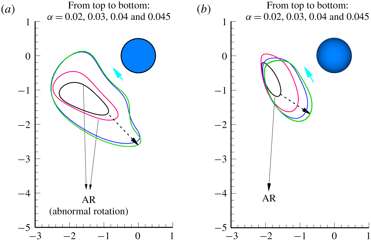
The comparison between the 2-D and 3-D computations was first made for the relative trajectories at  $Ga=13$, as shown in figure 22. For fixed
 $\unicode[STIX]{x1D6FC}$, the orbit of relative trajectory is larger for the 2-D case, implying that the circular cylinders oscillate more strongly than the spheres under the same conditions. In particular, when the rotation of a heavy particle changes sign, the orbit jumps in size for both cases, though this jump is much more noticeable for the cylinders. For instance, as
 $\unicode[STIX]{x1D6FC}$ increases from 0.03 to 0.04, the oscillation amplitude in the direction of gravity increases by nearly 90 % for the cylinders. By contrast the amplitude increases by just 48 % when
 $\unicode[STIX]{x1D6FC}$ increases from 0.02 to 0.03. In addition, the circular cylinders oscillate in the horizontal direction almost as strongly as in the vertical direction. However, the periodic motion of the spheres is mainly in the vertical direction (see also figure 16). Hence, the direction of gravity dominates oscillation of spheres.
Relative particle trajectories for the (a) 2-D and (b) 3-D computations at  $Ga=13$.

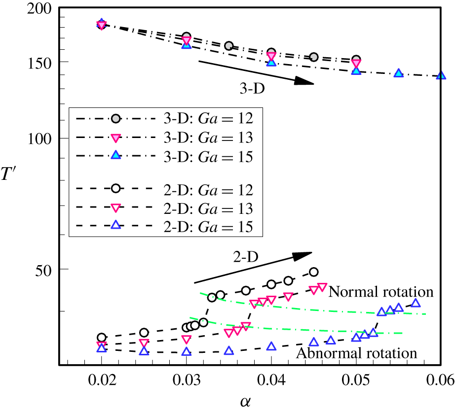
More importantly, the sudden jump in the relative trajectory leads to an abrupt increase in the particle period for the circular cylinders, as shown in figure 23. It takes more time for the particles to complete a larger closed orbit. For instance, the value of  $T^{\prime }$ increases by 13 % as
 $\unicode[STIX]{x1D6FC}$ is increased from 0.037 to 0.038 at
 $Ga=13$, which, by contrast, increases only 2 % as
 $\unicode[STIX]{x1D6FC}$ is increased from 0.035 to 0.036. Regarding this, our recent work (Nie & Lin Reference Nie and Lin2019) showed that the discontinuity in the period occurs for a certain range of Ga in a narrow channel (for example,
 $10.5\leqslant Ga\leqslant 15$ for
 $L=5d$), which originates from the change in rotation sign for the heavy particle. The same behaviour is also observed at
 $Ga=12$ and 15 for the circular cylinders (figure 23). However, it seems that there is no discontinuous change in
 $T^{\prime }$ in the 3-D computations. Figure 23 also clearly shows that the period is much longer for the 3-D case. Taking
 $Ga=13$ for instance, the oscillation period is approximately 33 for
 $\unicode[STIX]{x1D6FC}=0.02$ for the circular cylinders, which is almost six times the corresponding period for the spheres. This further suggests that the oscillation is much faster and stronger for the circular cylinders (with larger limit cycles but shorter periods). Another significant difference is that
 $T^{\prime }$ increases with
 $\unicode[STIX]{x1D6FC}$ in the 2-D case for
 $Ga\leqslant 15$. However, the opposite is true for the 3-D case, although the relative trajectory of the spheres clearly enlarges with increasing
 $\unicode[STIX]{x1D6FC}$. This is further evidence that the spheres interact with each other differently from their 2-D counterparts.
Particle periods as functions of  $\unicode[STIX]{x1D6FC}$ for
 $Ga=12$, 13 and 15. The value of
 $T^{\prime }$ is normalised through
 $T^{\prime }=T/T_{0}$. The 2-D results were presented in our previous paper (Nie & Lin Reference Nie and Lin2019).

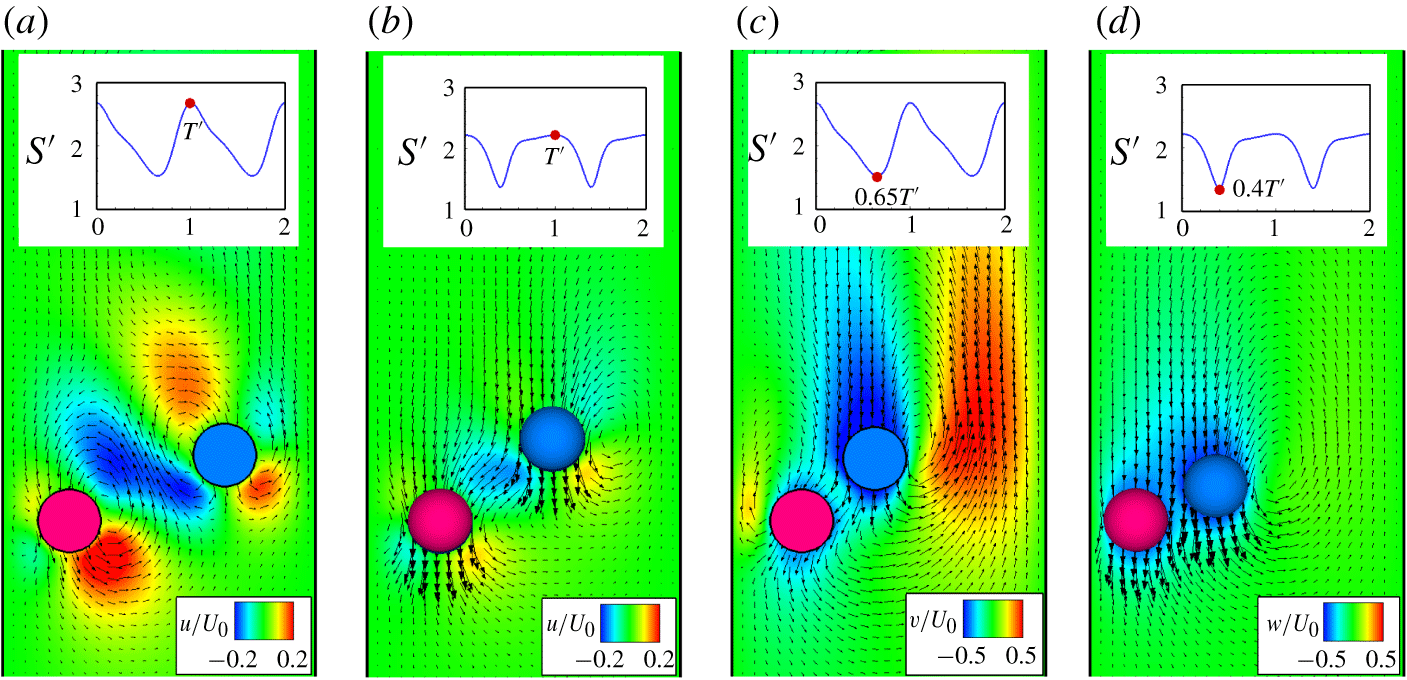
Figure 24 shows the simulated 2-D (a,c) and 3-D (b,d) instantaneous fluid velocities around the particles for  $\unicode[STIX]{x1D6FC}=0.03$ at
 $Ga=13$. For the 3-D case the results in the centreline plane are shown. The computations yield a very similar Reynolds number (
 ${\approx}$5.16) for both cases. Also shown in figure 24 are the contours of the horizontal (a,b) and vertical (c,d) fluid velocity components when the distance between particles reaches its maximum (a,b) and maximum (c,d). Under the same flow conditions, the fluid is much more strongly disturbed by the interacting cylinders in terms of the horizontal velocity below particles and between particles (figure 24a), and in terms of the vertical velocity behind particles (figure 24c). This agrees with the comparisons of the relative trajectories and periods in figures 22 and 23, respectively, considering the disturbance of the fluid to be its response to the particle motion. Furthermore, compared with the 2-D case, the vertical fluid velocity predominates over the horizontal component in the 3-D flow fields, which is also consistent with the observation that the spheres oscillate more strongly in the direction of gravity (see also figures 16 and 22). Another significant difference in figure 24 is that the 2-D flow fields have more noticeable recirculation zones, which result from the strongly interacting cylinders. The recirculation zones induce high shear-rate flow, which prevents the particles from coming close to the walls or to each other. The tendency becomes more significant at higher Reynolds numbers. There are no recirculation zones between the particles in the 3-D flow fields, which are similar to those in figure 14. This may be responsible for the opposite behaviours of the period with increasing
 $\unicode[STIX]{x1D6FC}(Re_{T})$ for the 2-D and 3-D cases in figure 23. Moreover, simulations show that at high Ga (like
 $Ga=25$) the period of the spheres first decreases as
 $\unicode[STIX]{x1D6FC}$ increases (
 $\unicode[STIX]{x1D6FC}\leqslant 0.04$), then increases with
 $\unicode[STIX]{x1D6FC}$. The increasing tendency at large
 $\unicode[STIX]{x1D6FC}$ seems primarily due to the noticeable recirculation zones between the spheres and walls as well as those between the spheres, as shown in figure 15.
Comparison of the 2-D (a,c) and 3-D (b,d) fluid velocities for  $\unicode[STIX]{x1D6FC}=0.03$ at
 $Ga=13$ obtained from the simulations. The terminal Reynolds number (
 ${\approx}$5.16) is very similar for both cases. Panels (a,b) show the magnitude of the horizontal velocity, and (c,d) the magnitude of the vertical velocity. Each upper panel is a time history plot of relative particle distance. Panels (a,b) are at the time the distance between particles is at its maximum, while (c,d) are at minimum particle separation.

5 Conclusions
The 3-D LBM was used to simulate the sedimentation of two spheres with different densities in a  $L=5d$ square tube for the Galileo number range 5–25. The non-dimensional parameter
 $\unicode[STIX]{x1D6FC}$ was introduced to adjust the ratio of the density difference between the spheres to the fluid density. The two spheres were released initially from rest in the centreline plane of the tube. Equal spheres (
 $\unicode[STIX]{x1D6FC}=0$) always reach a steady state in the centreline plane over the Ga range studied. However, for
 $\unicode[STIX]{x1D6FC}>0$ our sedimentation system has more complex dynamical behaviour because of the interactions between the heavy and light spheres. Some concluding remarks follow.
The spheres move to the diagonal plane or reverse–diagonal plane of the tube at low Ga, achieving either a steady state (small  $\unicode[STIX]{x1D6FC}$) or a periodic state (large
 $\unicode[STIX]{x1D6FC}$). At high Ga, however, the spheres are likely to oscillate in the centreline plane where they are released initially. This is possibly because a high-pressure zone forms between the heavy sphere and nearby wall at low Ga, while low-pressure zones appear on the sides of the sphere. This situation is more significant when the heavy sphere comes closer to the wall. Owing to this unique pressure distribution, the heavy sphere moves to either of its sides, namely, the diagonal plane or reverse–diagonal plane. The hydrodynamic interactions force the light sphere to leave the centreline plane. At high Ga, however, this situation reverses. The high-pressure zones on the sides of the heavy sphere prevent it from leaving the centreline plane.
We examined the effects of the Reynolds number on the (averaged) distance between spheres ( $S^{\prime }$) for particle motion in the (reverse–) diagonal plane. Increasing
 $\unicode[STIX]{x1D6FC}$ or Ga leads to an increase in
 $Re_{T}$, which, however, shows opposite effects on the variation of
 $S^{\prime }$ with
 $Re_{T}$. This is because the heavy sphere comes closer to nearby walls at larger
 $\unicode[STIX]{x1D6FC}$ when Ga is fixed, resulting in stronger tube-blocking effects. This suppresses the wake of the heavy sphere. As a consequence, the light sphere comes nearer to the heavy one. The opposite is seen when increasing Ga while holding
 $\unicode[STIX]{x1D6FC}$ constant.
We presented the limit cycles, relative trajectories and flow features to illustrate the periodic motion of the spheres in the centreline plane. At low Ga, the oscillations of the light sphere are stronger irrespective of  $\unicode[STIX]{x1D6FC}$. By contrast, at high Ga the heavy sphere oscillates much more strongly than the light one when
 $\unicode[STIX]{x1D6FC}$ is large. At low Ga there is an abrupt enlargement in the relative trajectories resulting from the change in rotation sign of the heavy sphere. This behaviour becomes insignificant as Ga increases.
Finally, we compared the 2-D and 3-D computations for this sedimentation system. The relative trajectories show that the oscillations of the circular cylinders (two-dimensional) have much higher amplitude and frequency under the same flow conditions. The comparison also shows that the circular cylinders oscillate almost as strongly in the horizontal direction as in the vertical direction. By contrast, the spheres oscillate predominantly in the direction of gravity. These observations are further confirmed by comparing the flow features from the 2-D and 3-D computations. The two-dimensional relative trajectories also abruptly enlarge when the heavy particle rotation changes sign. This further leads to a sudden increase in the period of the circular cylinders, which does not happen for the spheres. Another significant difference is that, for the 2-D case, the particle period increases as  $\unicode[STIX]{x1D6FC}$ increases at fixed Ga, while the opposite is true for the 3-D case. The recirculation zones generated by the strongly interacting circular cylinders prevent the particles from coming toward each other or the walls. This may be responsible for the increase in period with increasing
 $\unicode[STIX]{x1D6FC}$ for the 2-D case.
Acknowledgements
This work was supported by the National Natural Science Foundation of China (grants 11632016 and 11972336) and the National Key Research and Development Program of China (grant 2017YFB0603700).
Declaration of interests
The authors report no conflict of interest.