

Introduction
Glaciers and ice caps outside the Greenland and Antarctic ice sheets comprise approximately 4% of the area and around 0.5% of the volume of land ice. If they were to melt completely, they would raise global sea levels by approximately 0.5m (Dyurgerov and Meier Reference Dyurgerov and Meier1997). Small glaciers and ice caps are more responsive to climate change than are large ice sheets, and the melting of such small ice masses is believed to have contributed 0.2 to 0.4mmyr−1 to global sea level changes during the 20th century (Arendt and others Reference Arendt, Echelmeyer, Harrison, Lingle and Valentine2002), compared with 0.15mmyr−1 for Greenland, 0.2mmyr−1 for west Antarctica and possible balance, though with large uncertainties, for east Antarctica (Thomas and others Reference Thomas, Rignot, Casassa, Kanagaratnam, Acuña, Akins, Brecher, Frederick, Gogineni, Krabill, Manizade, Ramamoorthi, Rivera, Russell, Sonntag, Swift, Yungel and Zwally2004). Small ice masses will also continue to make a significant contribution to sea level rises during the 21st century (Church and others Reference Church, Gregory, Huybrechts, Kuhn, Lambeck, Nhuan, Qin, Woodworth, Houghton and Yihiu2001). The range of uncertainty in these estimates is large, and part of this stems from the paucity of measurements of glacier mass balance globally, especially at high latitudes (Arendt and others 2002). However, part of the uncertainty also relates to the extrapolation of sparse, point-based direct measurements of glacier mass balance, or of point measurements of height change between known time intervals, to give areal estimates of total melt. Such extrapolations usually assume that the measured mass balance is applicable to some elevation range across the glacier, implicitly assuming that only height will determine mass balance, and effectively neglecting any spatial variability in mass balance within given elevation bands. Recent research (Hagen and others Reference Hagen, Etzelmüller and Nuttall2000; Rippin and others Reference Rippin, Willis, Arnold, Hodson, Moore, Kohler and Björnsson2003) has cast some doubt on the validity of these assumptions.
More recently, measurements of changes in surface elevation of glaciers have begun to be made by comparing digital elevation models (DEMs) compiled at different times. Suitable DEMs can be constructed from a number of types of data, including GPS survey (Rippin and others 2003), stereophotography (Reinhardt and Rentsch Reference Reinhardt and Rentsch1986; Andreassen and others Reference Andreassen, Elvehøy and Kjøllmoen2002), radar interferometry, spaceborne radar altimetry (Davis and others Reference Davis, Li, McConnell, Frey and Hanna2005; Johannessen and others Reference Johannessen, Khvorostovsky, Miles and Bobylev2005) and laser profiling or LiDAR (Krabill and others Reference Krabill, Thomas, Martin, Swift and Frederick1995; Baltsavias and others Reference Baltsavias, Favey, Bauder, Bosch and Pateraki2001). Recent technological improvements in airborne LiDAR technology have substantially enhanced the available precision, horizontal resolution and data rate (Arnold and others Reference Arnold, Rees, Devereux and Amable2006a).
The surface height change of a glacier over a given period is the result of both the surface mass balance, and the surface mass flux divergence field (Hubbard and others Reference Hubbard, Willis, Sharp, Mair, Nienow, Hubbard and Blatter2000). Like surface height change, the surface velocity field can be determined by in situ point-based measurements (typically by repeated GPS surveying of the positions of stakes embedded in the glacier surface), though again there is the problem of sparse data. In this case, remotely-sensed imagery has also proved advantageous. If characteristic surface features such as crevasses, moraines or foliation can be recognised in a pair of co-registered images separated in time, these features can serve as markers from which the surface displacement can be determined (Hambrey and Dowdeswell Reference Hambrey and Dowdeswell1994). The features themselves can be identified manually (Lucchitta and others Reference Lucchitta, Mullins, Allison and Ferrigno1993) or by examining the cross-correlation between the two images (Scambos and others Reference Scambos, Dutkiewicz, Wilson and Bindschadler1992). The recent improvement in the technical capabilities of airborne LiDAR referred to in the preceding paragraph has raised the interesting possibility that LiDAR data could be used as a substitute for imagery (whether optical or radar), with features of the surface topography being used as markers. This approach has already been demonstrated in principle (Abdalati and Krabill Reference Abdalati and Krabill1999) for comparatively large-scale topographic features (the data were gridded to a resolution of 32 m) on a fast-flowing ice stream in Greenland, so the idea is not unprecedented. So far as we are aware it has not, however, been applied to metre-scale topographic features on small glaciers. The aims of this paper are to investigate the scope of high-resolution airborne LiDAR for measuring glacier mass balance and dynamics, based on a case study of a small high-arctic glacier.
Study site and LiDAR data collection
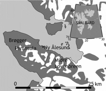
The investigation was carried out on Midre Lovénbreen. This is a small alpine-type polythermal glacier in Svalbard (Rippin and others 2003). It is around 5 km long, occupying an area of around 4 km2, and is logistically convenient being located within 5 km of the research facilities at Ny ålesund (Fig. 1). It has been extensively studied, with a mass balance stakeline established by the Norsk Polarinstittut since 1967, and has been the focus of glaciological research at the Scott Polar Research Institute, Cambridge, for nearly a decade. LiDAR data were collected over Midre Lovénbreen on 9 August 2003 and just under two years later, on 5 July 2005. Except for the very uppermost parts of the glacier, its surface was free of snow on both occasions. The instrument used for the data collection on both occasions was an Optech ALTM3033 LiDAR belonging to the Unit for Landscape Modelling (ULM) of the University of Cambridge. It was flown on board the Dornier 228 aircraft belonging to the Airborne Research and Survey Facility (ARSF) of the Natural Environment Research Council (NERC). Details of the data acquisition in 2003 are given by Arnold and others (Reference Arnold, Rees, Hodson and Kohler2006a); the 2005 acquisition followed a very similar procedure. In each case the data were collected at a mean density of around 0.8 points per square metre (that is around 3–4 million heights were recorded over the glacier itself), and then they were gridded to a resolution of 2m.
Location of Midre Lovénbreen and Ny ålesund, Svalbard.

Elevation change and mass balance
Before attempting to derive estimates of elevation change from the difference of the two DEMs, we assessed accuracy with which such a change could be measured. This has two components: the inherent precision with which the LiDAR can determine range, and the accuracy of the registration between the two DEMs. The combined effect of these components is given by equation (1)

where σ is the uncertainty in the estimate of an elevation difference, σ0 is its value over a horizontal surface, m is the magnitude of the surface slope, expressed as a fraction, and a is a constant with the dimension of length that combines the registration error between the DEMs, the grid spacing and the pointing error in the LiDAR. In order to estimate the values of σ 0 and a, the two DEMs were masked in to eliminate all areas except exposed rock, which could be assumed to have undergone no change in elevation between 2003 and 2005. Elevation differences were extracted from the DEMs, values of m were calculated from the 2005 DEM, and the data were used to fit the model parameters. Slightly more than 300,000 data points were processed, giving best-fit values of σ0=0.38±0.01m and a=0.63±0.01m. The mean elevation difference between the bare-rock areas of the two DEMs was 0.7mm. Thus we conclude that elevation differences measured by comparing the two DEMs have no significant systematic error, and random errors of at most about 0.38m for the gentle slopes of the glacier surface. The random errors may be smaller than this, owing to the significantly higher signal-to-noise ratio of LiDAR returns reflected from the high-albedo glacier surface compared with the low-albedo rock surface. A previous analysis of elevation accuracy in the 2003 DEM suggested that a typical value of the rms uncertainty over the glacier was around 0.15m, so the difference between two DEMs would be expected to be determined with an uncertainty √2 times as large, or around 0.21m.
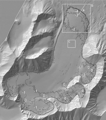
Contours of elevation change 2003–2005 superimposed on a slope-shaded rendering of the 2005 DEM. The heavy black line is the approximate boundary of the glacier. (a) Location of the transect in figure 3; (b) Location of the snout area shown in Fig. 4; (c) Location of the extract shown in Fig. 5. The image shows an area of 4080m (N-S) by 3600m (E-W); north is at the top.

Fig. 2 shows the elevation difference over the glacier surface from 2003 to 2005. It can be seen that this change is negative almost everywhere on the glacier, except for a few small regions towards the eastern and southeastern edges. Over most of the surface the elevation decreased by between 1 and 2m, although decreases of 4m and more were observed towards the glacier snout, especially on the eastern side. The average change over the whole glacier was −1.37m, with a negligibly small uncertainty. This can be converted to the water equivalent (w.e.) by multiplying by the ratio of the density of glacier ice to that of water, which we take as 0.90 to allow for presence of air bubbles and fractured ice near the surface of the glacier (Miller and Pelto Reference Miller and Pelto1999). This gives a value of −1.23m w.e. The measurement period was 696 days or around 1.91 years, and included two accumulation periods but less than two ablation periods, so the annualised spatially averaged mass balance can be deduced to have been more negative than −0.62myr−1 w.e.
Change in area and marginal retreat
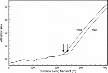
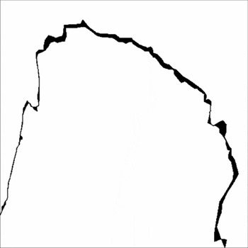
The lower boundary of the glacier is easily delineated in the DEMs through the abrupt change of slope bet-ween the forefield and the glacier (Fig. 3). By manually tracing the boundary in the 2003 and 2005 DEMs, the retreat of the glacier is shown (Fig. 4) to be predominantly from the northward and eastward facing parts of the snout. Surface energy balance modelling has shown that these areas are subject to very high potential solar radiation receipt due to their slope, aspect and exposure (Arnold and others 2006b) and this would seem to be the main reason for the concentration of retreat in these areas. The area deglaciated is 0.028 km2. The average width of the retreat is 13.7m over the north-facing part of the margin.
Colocated transects across the glacier snout. The boundary of the glacier (arrows) is indicated by a pronounced change in slope. The location of the transect is shown in Fig. 2.

Areas of the glacier snout in 2003 from which the ice had retreated by 2005. The map covers an area 480m square and its location is shown in Fig. 2.

The glacier margins are more difficult to discern at higher altitudes since the change of slope is not so abrupt, although the contrast between the smooth ice surface and the rougher surface of the exposed rock (Fig. 2) provides some contrast on which to base a manual delineation. On this basis, the area of the glacier in 2003 is estimated as 4.86 km2. No significant marginal retreat is detectable from the slope-shaded DEMs of 2003 and 2005 except at the snout.
Surface velocity estimates by feature tracking
The ability of accurate, high-resolution LiDAR data to resolve surface features on a glacier such as meltwater channels and (possibly snow-covered) crevasses has already been demonstrated (Arnold and others 2006a). The ability of these features to provide the basis on which surface velocities can be calculated depends on their persistence over time, and whether they possess sufficiently distinctive spatial variation to allow their positions to be unambiguously determined.
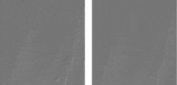
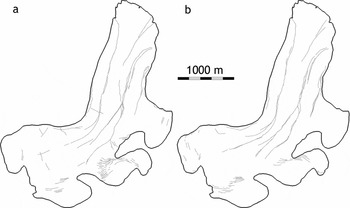
Whether feature-tracking is performed manually or automatically, the DEMs must first be processed to resemble an image. This was done by applying a linear gradient filter to the DEMs to mimic approximately the effect of illuminating the surface from the northwest. This procedure enhances the appearance of linear features unless they happen to run in a northwest-to-southeast direction, and produces reasonably realistic pseudo-images from the DEMs (Fig. 2). Fig. 5 shows extracts from the middle of the glacier that demonstrate that active and relic meltwater channels are indeed recognisable, and that their general form is persistent over the two-year interval. As a further preliminary to feature-tracking, these linear features were traced manually in both slope-shaded DEMs (Fig. 6).
256m square extracts from the slope-shaded 2003 (left) and 2005 (right) DEMs, showing a system of meltwater channels. The location of the extracts is shown in Fig. 2. North is at the top.

Manually delineated lineaments in the 2003 (a) and 2005 (b) DEMs. North is at the top.

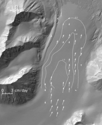
A semi-automated procedure for feature-tracking was implemented as follows. The slope-shaded and manually delineated DEMs were divided into 128×128 pixel tiles. The corresponding tiles for 2003 and 2005 were compared by Fourier-transform based cross-correlation (Bernstein Reference Bernstein and Colwell1983), and the resulting correlogram inspected visually to determine whether it contained a well-defined maximum and, if so, to find its coordinates. These coordinates define the shift, in pixels, between the two image tiles. Where a shift could be determined by both methods (slope-shaded and manually delineated), and the shifts were in agreement to within ±1 pixel, it was accepted as a valid estimate of the displacement. The results of this analysis are shown in Fig. 7, superimposed on speed contours derived by Rippin (Reference Rippin2001) from in situ measurements over the year 1998. The figure shows many successful matches on the lower half of the glacier, particularly on the eastern side, all derived from meltwater channels. The calculated speeds show good general correspondence (r 2=0.446, n=31, p=0.00002) with the speeds measured by Rippin, typically in the range 1–2 cm per day or around 7–14m between the 2003 and 2005 acquisitions.
Motion vectors determined by semi-automated Fourier-transform correlation (arrows) compared with speed contours derived from in situ measurements in 1998. The contours are labelled in units of cm/day.

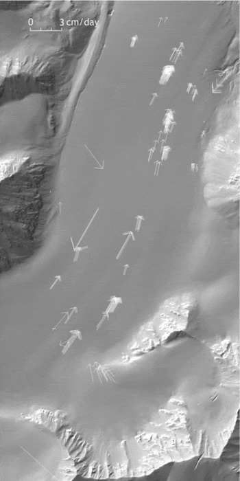
A fully-automated procedure was also investigated. This used VisiCorr, an implementation of the ImCorr algorithm (Scambos and others 1992) for Microsoft Windows developed by T. Benham of the Scott Polar Research Institute (Dowdeswell and Benham Reference Dowdeswell and Benham2003). The algorithm was applied to the slope-shaded DEMs. A typical set of output motion vectors determined by the application of this algorithm is shown in Fig. 8. Again, most matches are found on the lower half of the glacier, with more on the eastern than the western side, although this algorithm also succeeded in obtaining realistic matches from one of the crevasse fields. Most of the velocities are at least qualitatively consistent with those of Fig. 7, although clearly some blunders are also committed by the algorithm, for example up-glacier flow vectors. However, it is noted that the feature-tracking algorithm has seven adjustable parameters, and that the pre-processing of the DEMs also involves some choice of parameters, so there is probably considerable scope for refinement.
Motion vectors determined using fully-automated Fourier-transform based image correlation.

Discussion
Mass balance
The annual mass balance derived in this work, ≤−0.62±0.02myr−1 water equivalent, is considerably more negative than estimated from in situ measurements. Field measurements have shown values of around −0.35myr−1 averaged over the period 1977–1995 (Lefauconnier and others Reference Lefauconnier, Hagen, Ørbaek, Melvold and Isaksson1999), and similar values have been deduced for the period 1997–2003 (J. Kohler, personal communication, 2005). On the other hand, a recent determination of the mass balance of Midre Lovénbreen based on the analysis of two DEMs (from 1977 and 1995) found an average value of −0.61±0.7myr−1 w.e. (Rippin and others 2003). This is entirely consistent with our value although very imprecisely specified. In fact, Rippin and others (2003) probably overestimated the uncertainty in their mass balance calculation by assuming that errors in the DEMs were spatially correlated over the whole glacier. A more reasonable but still cautious assumption would be that the correlation lengths were around 500m, giving an uncertainty in the 18-year average of around 0.17myr−1 w.e. This would still be consistent with the present value. As Rippin and others (2003) pointed out, there is also evidence from the glacier Finsterwalderbreen in southern Svalbard of a substantial discrepancy between in situ and DEM-derived mass balance estimates. In that case, the ratio of the in situ mass balance estimate to that from DEMs was around 0.7, comparable to the value of 0.55 for Midre Lovénbreen.
In situ measurements of the mass balance of Midre Lovénbreen for the period 2003–2005 are not yet available, so a direct comparison of the two methods is not possible. The apparent discrepancy could possibly be explained if the temperature were higher and the precipitation were lower than average during this period. An annual mass balance of −0.62m w.e. is within the range of around −1 to +0.1m deduced from in situ measurements over the period 1968 to 2000 (Kohler and others no date), and indeed the highest temperature ever recorded at Ny ålesund occurred in July 2005 (18.7 C on 7 July; data from the Norwegian Meteorological Institute). However, regression of mass balance estimates from in situ measurements against temperature and precipitation data recorded at Ny ålesund does not suggest that the mass balance over the period from August 2003 to July 2005 was significantly different from the average over the previous two decades. The regression-estimated annualised mass balance for the period 2003–2005 is −0.36m w.e.
Another possible explanation for the discrepancy between the present estimate of the mass balance and those derived from in situ measurements is that we could have significantly overestimated the mean density of the ablated material. This is, however, unlikely. The glacier surface during the 2003 LiDAR acquisition was almost completely free of snow, and entirely so over its lower half where most of the loss of volume occurred. Although we did not measure the surface density of the glacier in either year, we performed various other physical measurements that involved penetrating the surface, and it was obvious that it consisted overwhelmingly of ice rather than firn. Even if the ablated material was 100% firn, with an assumed density of 0.8 times that of water, the annualised mass balance would become −0.55myr−1 w.e. Correction for the presence of a thin covering of snow during the 2005 acquisition (this was somewhat earlier in the season) would, if anything, mean that our estimate of the annualised mass balance is insufficiently negative.
If the discrepancy is indeed real, it suggests that estimates of the mass balance of Midre Lovénbreen, and perhaps other glaciers, from in situ measurements may need to be treated with caution. Two possible sources of error can be identified. Firstly, the elevation change recorded at a mass balance stake may not be sufficiently representative of the elevation change at other points on the glacier at the same elevation. In other words, the mass balance may exhibit significant spatial variability, beyond that explained by elevation alone. Secondly, the spatial distribution of stakes may not be sufficient to characterise the dependence of mass balance on elevation. This relationship is not linear, as is shown by both the LiDAR data and energy balance modelling, particularly towards the glacier snout. These possibilities are both currently the subject of further investigation.
Change in area
Our calculated rate of retreat of the glacier snout of 13.7m over the 1.9 years between the two DEMs gives an annual average of 7.2myr−1. This is similar to the value of 8.3myr−1 estimated by Rippin and others (2003), and consistent with the suggestion that the margin of Midre Lovénbreen has retreated by around 1000m since 1890 (Hansen Reference Hansen1999). Since no significant marginal retreat is observed other than in the snout area, it is concluded that the total reduction in the area of the glacier between 2003 and 2005 was just the 0.028 km2 measured at the snout. This gives an annual rate of loss of around 0.015 km2 yr−1, considerably below the value of 0.05 km2 yr−1 estimated by Rippin and others (2003) for the period 1977 to 1995. This suggests either that the glacier was retreating rather rapidly all around its margin (the rate would need to be something like 6myr−1) from 1977 to 1995 but has now stopped, or that the value of 0.05 km2 yr−1 was somewhat overestimated. In view of the difficulty of delineating the margin other than at the snout, and of the apparent regularity of the glacier's behaviour before and after 1995, the latter explanation seems more plausible. However, DEM data, even at the high resolutions afforded by systems such as the Optech ALTM3033, are almost certainly not optimal for measuring the spatial extent of glaciers, and high-resolution visible imagery would be preferable.
Surface velocity
The results of the investigation of feature-tracking are promising. The semi-automated method shows that reliable and consistent velocity vectors can be extracted from meltwater channels, and that these retain their identity over at least two years. The attempt to extract velocities using a fully automated feature-tracking algorithm was also largely successful, producing mostly believable velocities from both meltwater channels and crevasses, although it also generated some obvious blunders. These could perhaps be reduced in number, or avoided altogether, by adjusting the parameters of the algorithm. Neither approach yielded velocity vectors over the whole of the glacier's surface. The upper part of the glacier was not represented, and we may speculate that this is a consequence of there being fewer and weaker features in this region.
Conclusions
High-resolution, accurately calibrated airborne LiDAR is capable of generating DEMs of sufficient quality that they can be used to calculate glacier mass balance even when the time interval between them is as short as two years (and perhaps even less than this). The other aspect of geometrical change that is well determined by such DEMs is the retreat or advance of the glacier snout. Glacier area is rather harder to determine from a DEM alone. The ability of high-resolution DEMs to resolve surface topographical features in sufficient detail to serve as features that can be tracked to deduce velocity has been verified, although the optimum combination of parameters for automating the process has yet to be established.
The specific results for Midre Lovénbreen, expressed as annual averages over the period 2003 to 2005, are that its mass balance was around −0.62m w.e., its snout retreated by around 7.2m, and that its area decreased by 0.015 km2, accounted for by the retreat of the snout. The horizontal surface displacement in the middle of the glacier was around 3.5 to 7m. The area of the glacier in 2003 was estimated to be 4.86 km2. Some of these results are consistent with previous work and some are not. The most significant discrepancy is the mass balance figure, which is substantially more negative than that estimated from mass balance stake measurements. This, and other evidence, suggests that the spatial variability of mass balance may be greater than previously realised and that estimates based on a comparatively few in situ measurements may need to be treated with caution.
Acknowledgements
LiDAR data were collected by the UK Natural Environment Research Council (NERC)'s Airborne Research and Survey Facility (award ARSF 03/04) and the University of Cambridge Unit for Landscape Modelling. Fieldwork logistics were provided by the NERC Arctic Research Station at Ny ålesund. Funding was provided by the University of Cambridge and by Christ's and St John's Colleges, Cambridge. We gratefully acknowledge the assistance of Nick Cox and his colleagues at the NERC Arctic Research Station, Jack Kohler for allowing us to use his in situ mass balance data in advance of publication, Toby Benham for providing the VisiCorr software, and an anonymous reviewer for suggestions that have materially improved this paper.