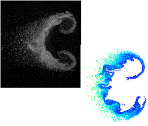

1. Introduction
Hydrodynamic instabilities (HIs) are widespread in natural and engineering phenomena. The study of HIs is concerned with the process by which a laminar flow transitions to a turbulent one. For the shock-driven flow considered in this paper, a family of related HIs is involved, including the Kelvin–Helmholtz (KHI), Rayleigh–Taylor (RTI) and Richtmyer–Meshkov (RMI) instabilities. The KHI forms as a result of velocity difference, shear, over a fluid interface. A RTI is generated when density and pressure gradients are misaligned with the heavy fluid resting above the light fluid, in relation to a constant acceleration, e.g. gravity. This misalignment results in the formation of baroclinic vorticity. The RMI is closely related to the RTI, and can be viewed as the impulsive i.e. shock wave, acceleration limit of the RTI. The RMI is unstable in any orientation of the density gradient. These instabilities can occur simultaneously and KHI and RTI form in the late stages of the RMI. The inclusion of multiphase effects will complicate the evolution of these instabilities but the basic mechanisms of initiation will be similar.
1.1. Shock-driven multiphase instability
The shock-driven multiphase instability (SDMI) is a HI for multiphase fluids that is similar in many ways to the RMI. It evolves at large scales (relative to the particle size) and is driven by the properties of the bulk, multiphase fluid mixture. In a multiphase fluid mixture the continuous phase (larger volume fraction) is referred to as the carrier phase, a gas here, while the discrete phase (smaller volume fraction) is referred to as the particle phase, liquid droplets here. One way for the SDMI to arise is from the impulsive acceleration (by a shock wave) of a perturbed interface (steep gradient) between multiphase fluid mixtures of different effective densities. Instability may also arise from a gradient in particle-to-gas velocity equilibration time (McFarland et al. Reference McFarland, Black, Dahal and Morgan2016). The effective density is defined as the total mass (particles and gas) divided by their combined volume. The carrier phase density may be equal across the interface with only the dispersed phase creating a difference in effective density, as seen in this work.
The RMI may be regarded as the limit of the SDMI as the length scale (size) of the particle goes to zero. In this case the particles will follow the carrier phase exactly and the mixture will behave as a continuous fluid with the evolution following that of an RMI. In the RMI, misalignment of the density and pressure gradients drives the deposition of baroclinic vorticity. In the SDMI, the vorticity deposition mechanism is the same but is modified by the finite equilibration time between the particle and carrier phases.
SDMIs have been recognised in natural large-scale phenomena, such as the Crab nebula, interstellar dust activities near asymptotic giant branch stars and in engineering applications such as high-speed multi-phase combustion in scram-jet engines and explosive dispersal of particles.
The effective density gradient at the interface is quantified by an effective Atwood number,  $A_e$, defined as the ratio of the difference in two regions’ effective densities to their sum
 \begin{equation} A_e=\frac{\rho_{e2}-\rho_{e1}}{\rho_{e2}+\rho_{e1}}\end{equation}
In (1.1),  $\rho _{e1}$ and
 $\rho _{e2}$ are the effective densities of the surrounding fluid and the interface fluid, respectively. The effective density is a function of the gas volume fraction or void fraction,
 $\epsilon$, carrier gas density,
 $\rho _g$, and the particle material density,
 $\rho _p$,
 $\rho _{e2}={\rho _{p}(1-\epsilon )+\rho _{g}\epsilon }$.
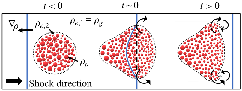
The distribution of particle properties, e.g. sizes and positions, plays a significant role in the SDMI. A simple schematic of the SDMI evolution for a circular interface is shown in figure 1. Here, the three basic ingredients for an SDMI are shown; a pressure gradient, created by the incident shock wave, a gradient in effective density, created by the multiphase fluid interface, and a misalignment between the two, created by circular interface shape.
SDMI's evolution in the shock tube.

1.2. Gas–particle coupling
The large-scale formation of the SDMI depends on particle-scale transport of momentum, energy and mass. Of these, momentum transfer has the largest effect. Energy transfer has a smaller effect, usually cooling the gas due to the high heat capacity of the particle phase. Mass transfer creates additional complexities, having a strong effect on the temperature of gas (due to thee latent heat of phase change), and will be considered in another section. Here we note that we use both the terms ‘particle’ and ‘droplet’ when discussing the dispersed phase, but reserve the later term for describing effects unique to a liquid dispersed phase, i.e. evaporation and breakup.
For momentum transport, the simple drag model considers a spherical rigid particle with size,  $d$, mass,
 $m_p$, and velocity,
 $\boldsymbol {v_p}$ in a gas with viscosity,
 $\mu _g$, and velocity,
 $\boldsymbol {v_{g}}$. The particle Reynolds number is calculated as
 $Re = (\rho _{g} v_{pg} {d})/\mu _{g}$, where
 $v_{pg}$ is the magnitude of the particle velocity relative to the gas. The force on a particle is then
 $F_d = m_p f_D (\boldsymbol {v_g}-\boldsymbol {v_p})$, where
 $f_D$ is a scalar component of the acceleration due to drag,
 $f_D=C_d(3/4)(\rho _g/\rho _p)(v_{pg}/d)$;
 $C_d$ is the drag coefficient for the particle and is calculated using various methods dependent on
 $Re$, particle volume fraction and Mach number (see Dahal & McFarland (Reference Dahal and McFarland2017) for more).
Energy transport, heat transfer, is found for a spherical particle by assuming heat to diffuse away from the particle, and modifying for convective heat transfer, by use of the Nusselt number,  $Nu$. The resulting equation, for the rate of change in particle energy, may be referred to as the Ranz–Marshall model (Ranz & Marshall Reference Ranz and Marshall1952). The
 $Nu$ may be found using various correlations dependent on the particle volume fraction,
 $Re$ and the Prandtl number,
 $Pr$.
For small droplets the continuum assumption may breakdown, and non-continuum effects should be considered. A measure for the degree of non-continuum effects can be made using the Knudsen number,  $Kn=Ma/Re \sqrt {\gamma {\rm \pi}/ 2}$, where
 $\gamma$ is the ratio of specific heats and Ma is the Mach number. Here
 $Kn$ represents the ratio of the molecular mean free path to the problem length scale of interest, the particle diameter in this case. As
 $Kn$ increases, above
 ${\approx }0.01$, non-continuum effects become important, and the continuum assumption begins to break down. In non-continuum flow regimes the rate of momentum and heat transfer is decreased.
The effects of energy and momentum transfer in a shock-driven multiphase field, where the particles are initially at rest and have a higher density and heat capacity than the gas, are to reduce the post-shock gas velocity and temperature. The reduction in gas velocity is the primary source of the SDMI. The rate at which momentum and, to a lesser degree, energy transfer occur has a large impact on the development of the SDMI. A time scale for velocity equilibration,  $t_v=\rho _p d^2/(18\mu _g)$ was proposed by Marble (Reference Marble1970). As
 $t_v$ increases, the particles lag further behind the gas flow. When
 $t_v$ becomes large relative to the characteristic hydrodynamic time scale, the particle lag begins to diminish the growth of the instability (McFarland et al. Reference McFarland, Black, Dahal and Morgan2016). This can be explained by the fact that the source of vorticity deposition lies with the particles. As the particles lag behind the flow, the vorticity source term advects with them and becomes misaligned, competing with the vorticity already deposited in the gas phase (Dahal & McFarland Reference Dahal and McFarland2017; Paudel, Dahal & McFarland Reference Paudel, Dahal and McFarland2018).
1.3. Evaporation
Phase change (evaporation in this work) is often neglected or prohibited in the study of SDMI and related shock-driven multiphase flows, due to the complexity of its effects on both energy transfer and particle size. Evaporation has a large impact on the gas and particle temperatures due to the latent heat of phase change. The resulting decrease in gas temperature, and corresponding decrease in gas density, alters the dynamics of the gas. This can induce additional fluid instability under secondary accelerations, such as the centripetal acceleration in strong vortices or subsequent shock waves (i.e. reflected waves) (Black, Denissen & McFarland Reference Black, Denissen and McFarland2017). In heterogeneous distributions of particles, evaporation occurs at different rates based on the local conditions. Evaporation occurs at higher rates along an interface between a droplet seeded region and a dry gas, and is highest where vortices create the largest slip velocity between the gas and particle phase (Paudel et al. Reference Paudel, Dahal and McFarland2018). In the case of a reacting vapour phase, the evaporation rate and vapour spatial distribution become important factors in determining the net reaction rate (Cheatham & Kailasanath Reference Cheatham and Kailasanath2005; Kailasanath Reference Kailasanath2006).
The classic, simple model for droplet evaporation considers a spherical liquid droplet with vapour diffusing between the droplet surface and the free stream (Crowe et al. Reference Crowe, Schwarzkopf, Sommerfeld and Tsuji2011). For convective conditions, this diffusion rate is modified using the Sherwood number,  $Sh$, which relates the convective mass transfer rate to the diffusive rate. Assuming constant conditions, it was found that the square of the droplet diameter,
 $d^2$, decreases linearly with time. This has come to be known as the d-squared model (Godsave Reference Godsave1953). Later, this work was extended the convective regime in the Ranz–Marshall model (Ranz & Marshall Reference Ranz and Marshall1952). Further models considered the effects of transient heating and non-uniform droplet and gas conditions (Abramzon & Sirignano Reference Abramzon and Sirignano1989). The effects of gas diffusion into the particle phase have been considered for high-pressure, reacting droplets by Aggarwal & Mongia (Reference Aggarwal and Mongia2002). An extensive comparison of droplet evaporation models for various hydrocarbons was presented by Sazhin et al. (Reference Sazhin, Kristyadi, Abdelghaffar and Heikal2006). Various evaporation models have been reviewed by Aggarwal & Peng (Reference Aggarwal and Peng1995).
Experimental data for evaporation of non-deforming droplets under steady and shock-driven conditions are widely available. Goossens et al. (Reference Goossens, Cleijne, Smolders and van Dongen1988) provided average size measurements for shock-driven evaporation of small ( $2\ \mathrm {\mu }$m) droplets. Hanson, Davidson & Hanson (Reference Hanson, Davidson and Hanson2007) developed a method for measuring the evaporation of droplets with large variation in size. Little experimental data exist, however, for larger deforming droplets undergoing evaporation, thus models for these combined effects remain scarce and/or unvalidated. Further, while the available models show that
 $Sh$ will decrease with increasing
 $Kn$ in non-continuum flow regimes, little data exist for the conditions considered in this work.
1.4. Breakup
Like evaporation, the effects of breakup are often neglected in shock-driven multiphase flows in order to simplify the problem. The effect of droplet breakup on the SDMI is to greatly reduce the size of droplets, increasing the rate of evaporation and velocity equilibration, yet it has not been considered in previous work on the SDMI. For reacting high-speed multiphase flows, such as those found in detonation engines and supersonic combustion ramjets, breakup is essential to converting droplet mass to vapour for reaction.
Droplet breakup is divided into various regimes based on the Weber number,  $We=\rho _g v_{pg}^2d/\sigma _p$), where
 $\sigma _p$ is the surface tension of the droplet. The stability of a droplet decreases as the
 $We$ increases, i.e. due to a larger relative velocity between the gas and droplet. There exists some disagreement in the literature on these regimes and their
 $We$ bounds. The regimes defined by Pilch & Erdman (Reference Pilch and Erdman1987) provide an early example of how breakup characteristics vary with increasing
 $We$ number. The stability of droplet can be increased with its viscosity and quantified by the Ohnesorge number,
 $Oh=\mu _p / \sqrt {\rho _p d \sigma _p}$, where
 $\mu _p$ is the droplet viscosity. At higher
 $Oh$, usually greater than 0.1, the critical
 $We$ for breakup and transition through each regime increases. For the conditions considered in this paper, the droplet breakup process is expected to fall primarily in the bag and bag and stamen regimes. A recent review of droplet breakup by Guildenbecher, López-Rivera & Sojka (Reference Guildenbecher, López-Rivera and Sojka2009) provides more extensive information on droplet breakup and Theofanous (Reference Theofanous2011) provides information of particular relevance to high
 $We$ droplets.
Droplet breakup does not begin instantly. Instead the droplet deforms for some time until breakup begins at the initiation time,  $t_{b,i}$. It then proceeds until completion at the total breakup time,
 $t_{b,t}$. Many breakup models provide non-dimensional times,
 $\tau _{b}=t/t_c$, based on a single characteristic breakup time,
 $t_{c}=d/v_{pg}(\rho _p/\rho _g)^{0.5}$ (Nicholls & Ranger Reference Nicholls and Ranger1969). Pilch & Erdman (Reference Pilch and Erdman1987) provides a single model for
 $\tau _{b,i}=t_{b,i}/t_c$ and different models for
 $\tau _{b,t}=t_{b,t}/t_c$ for five different
 $We$ regimes. The highest values for
 $\tau _{b,t}$ occur both at low
 $We$ and at high
 $We$, where it becomes constant at
 $\tau _{b,t}=5.5$. Hsiang & Faeth (Reference Hsiang and Faeth1992) provide a different model for breakup times based on data from shock-driven experiments. This model was found to have lower accuracy at low
 $We$, and later work from this group (Dai & Faeth Reference Dai and Faeth2001) provided improved estimates of
 $\tau _{b,t}$ at low
 $We$. Another estimate of
 $\tau _{b,i}$ was provided by the Taylor analogy breakup (TAB) model which treated the droplet as an oscillating spring–mass system, and finds similar values for
 $t_{b,i}$ (O'Rourke & Amsden Reference O'Rourke and Amsden1987). This model, however, treats breakup as an instantaneous event, disregarding
 $t_{b,t}$. Few models exist that describe the rate at which the droplet divides during the breakup time. An extension to the TAB model, the ETAB model (Tanner Reference Tanner1997), considers the number of droplet fragments (child droplets) to increase at an exponential rate. Dai & Faeth (Reference Dai and Faeth2001) do not provide a model, but instead a curve fit to data implying a similar exponential growth rate.
During the breakup process significant deformation of the droplet occurs. This greatly alters the drag force experienced by the particle. The droplet is assumed to deform from a sphere to an oblate spheroid of equal volume, where the axis is aligned with the vector of the relative gas velocity. The deformation of the particle is often measured by a ratio of the displacement of the equator to the original (spherical) droplet radius. In the TAB model, the parameter  $y=1-d_0/d_a$ is used, where
 $d_0$ is the unperturbed particle diameter and
 $d_a$ is the diameter at the equator. Liu, Mather & Reitz (Reference Liu, Mather and Reitz1993) proposed that
 $C_d$ would increase from that of a sphere (
 ${\sim }0.424$ at high
 $Re$) to that of a disk in cross-flow (
 ${\sim }1.52$), as
 $y$ increased from 0 to 1. The TAB model assumed that breakup then occurred when
 $y$ exceeded a value of 1 (O'Rourke & Amsden Reference O'Rourke and Amsden1987). Pilch & Erdman (Reference Pilch and Erdman1987) took a simpler approach suggesting constant drag coefficients for different regimes, while Hsiang & Faeth (Reference Hsiang and Faeth1992) and Dai & Faeth (Reference Dai and Faeth2001) (at low
 $We$) found a similar result to that used by Liu et al. Chou & Faeth (Reference Chou and Faeth1998) provided extensive data for the time history of
 $C_d$ for the core (parent) droplet throughout the breakup process, finding a rapid power-law-type decay in
 $C_d$ after the initiation of breakup.
While the rate of breakup and momentum coupling during breakup are important, the most significant factor to SDMI is the final, or child, droplet sizes. The breakup process produces fragments with a distribution of sizes and velocities, often spreading the resulting fragments away from the parent droplet. The fragment velocities are of great interest to combustion applications and are predicted in the TAB model (O'Rourke & Amsden Reference O'Rourke and Amsden1987; Tanner Reference Tanner1997). The resulting fragment size distribution, for the low  $We$ bag and bag-and-stamen regimes, has been approximated by a single log-normal or gamma distribution by Zhao et al. (Reference Zhao, Liu, Xu, Li and Lin2013). Chou & Faeth (Reference Chou and Faeth1998) predict two resulting droplet populations, from the bag and basal ring, with distinct distributions. For simplicity, a single representative diameter is often used in place of a continuous distribution of fragment sizes, such as the arithmetic, volume, Sauter and mass mean diameters. In the TAB model the child droplet size is described by the Sauter mean diameter, SMD or
 $d_{32}$, and is found by an energy balance considering the droplet deformation and surface tension energies. This was found to under-predict the final
 $d_{32}$; as a result, Tanner (Reference Tanner1997) proposed a new distribution with larger
 $d_{32}$ in the ETAB model. Hsiang & Faeth (Reference Hsiang and Faeth1992) proposed a model for child droplet
 $d_{32}$ in the shear breakup regime, based on fluid boundary layer in the liquid droplet. Chou & Faeth (Reference Chou and Faeth1998) and Zhao et al. (Reference Zhao, Liu, Xu, Li and Lin2013) proposed a single ratio (0.31) for
 $d_{32}/d_0$ at low
 $We$. For the bag and bag-and-stamen regimes, Wert (Reference Wert1995) proposed a model for
 $d_{32}$ based on fluid instability analysis, finding more accurate results at low
 $We$.
Few models have been presented for low  $Re$, small diameter (
 ${<}10\ \mathrm {\mu }$m), droplets, where velocity equilibration and evaporation are important, as are considered in this paper. Non-continuum effects, resulting from high
 $Ma$ or low
 $Re$, have been examined in some experimental works, finding that the breakup regimes are modified under high
 $Kn$ conditions citetheofanous2004aerobreakup. Recent simulation work (Syahdan Reference Syahdan2015) examined the effect of
 $Ma$ on droplet breakup finding that at supersonic
 $Ma$ the breakup process is delayed, and that the morphology of breakup is altered. These effects were shown to become significant at
 $Kn \approx 0.02$ but were not observed at
 $Kn \approx 0.002$. It is noteworthy that there is little consensus in the literature on many breakup characteristics, with few models for droplet drag during breakup, and little agreement on child droplet size models, especially in the low
 $Re$ or high
 $Ma$ regimes.
1.5. Paper overview
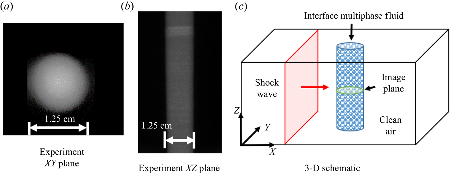
In this paper the effects of evaporation and breakup of droplets on the mixing induced by the SDMI are considered through simulations and experiments. Previous experimental results are compared with simulation results to test breakup and evaporation models and to gain insight into their effects on the SDMI. The experimental work was presented in a previous paper (Middlebrooks et al. Reference Middlebrooks, Avgoustopoulos, Black, Allen and McFarland2018). The experiments considered the evolution of a quasi-two-dimensional cylindrical region of droplet laden gas surrounded by dry gas (figure 2). Experimental measurements show the morphology of the droplet containing gas in a two-dimensional (2-D) slice from the midpoint of the cylinder as the SDMI evolves and mixes it with the surrounding gas. Two-dimensional simulations are run using new models for breakup and evaporation of the droplets. The evolution of the SDMI, interface morphology, is then compared between the simulations and the experiments and used to test models and provide new observations, at high temporal and spatial resolution unobtainable in experiments, of evaporation and breakup effects. In the following sections, the experimental apparatus is described, followed by the existing simulation capabilities and models. Then the evaporation models and effects are explored followed by breakup models and effects. Finally conclusions are provided based on the results of the previous sections.
Experimental initial conditions. (a) Mie scattering image of the initial particle field in the  $XY$ plane. (b) Mie scattering image of the initial particle field in the
 $XZ$ plane. (c) Three-dimensional schematic of the initial conditions.

2. Experimental methods
As this paper compares simulation with experimental results, a brief description of the experimental facility and conditions is provided in this section.
2.1. Experimental facility
The facility consists of a horizontally oriented closed shock tube made of cold-rolled steel with a total length of  ${\sim }9.5$ m and cross-section of
 ${\sim }14$ cm by
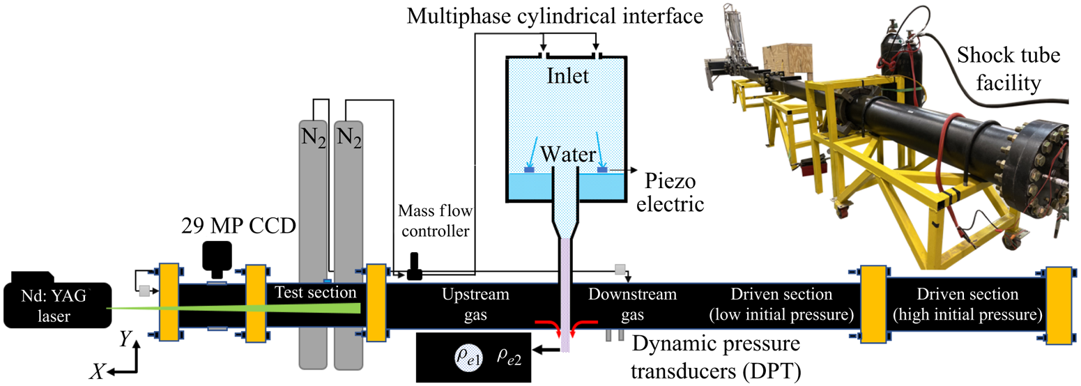
 ${\sim }14$ cm. The shock tube consists of three main sections: the driver, driven and test sections. The driver section stores the gas necessary to initiate the shock wave. The driven section is sufficiently large to provide time for the shock wave to become planar and steady before reaching the test section. Lastly, the test section holds the instruments necessary for data and image acquisition (figure 3).
Shock tube facility.

In the driver section, a pressure transducer and thermocouple are used to monitor the initial conditions and automatically start the shock initiation sequence. In the driven section, two dynamic pressure transducers are used to measure the shock velocity and post-shock pressure, and to trigger image acquisition. The driver and driven sections are separated with a diaphragm that is quickly ruptured by the rapid addition of additional gas through a fast, large valve. The rupture occurs in a predictable manner with the assistance of an ‘ $X$’ shaped knife that cuts the diaphragm as it fails. The test section holds the interface creation apparatus, and has five-window ports with camera mounts to image the interface at different times during its evolution. The test section is enclosed by the shock tube end wall.
The interface creation apparatus consists of a liquid reservoir, a gas mass flow controller and particle generators producing water droplets with a mean of  $1.7\ \mathrm {\mu }$m or
 $10.7\ \mathrm {\mu }$m diameter. The concentration and size distribution for the water droplets are obtained through an interferometry technique and verified with a mass retention technique. A custom-made filter captures droplets that are then weighted with a high precision balance to determine the droplet mass fraction and
 $A_e$. Finally, images are acquired using an Nd:YAG pulsed laser, providing 200 mJ per pulse at 532 nm, and a 29 MP interline charge-coupled device camera. More information can be found in Middlebrooks et al. (Reference Middlebrooks, Avgoustopoulos, Black, Allen and McFarland2018).
2.2. Experimental conditions and results from previous experiments
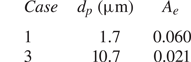
For this work, we compare our simulation results with the experimental cases 1 and 3 presented in Middlebrooks et al. (Reference Middlebrooks, Avgoustopoulos, Black, Allen and McFarland2018). To obtain a more accurate representation of the effective Atwood number, a closer examination of the reported experimental values was performed. For case 1, re-analysing the same data points utilised to calculate the previously reported value of  $0.07 \pm 0.002$, indicate that
 $A_e=0.06$ is a more accurate representation. This is because the water vapour present in the gas phase was initially neglected (water vapour is less dense than air). For case 3, the previously reported value was
 $A_e = 0.014 \pm 0.003$, with some outlying measurements being up to 0.022. Subsequent measurements were performed for case 3 with improved methods, finding a converged value of
 $A_e=0.021$. The improved values (table 1) were used in our simulations.
Experimental conditions simulated. Note: case 2 from Middlebrooks et al. (Reference Middlebrooks, Avgoustopoulos, Black, Allen and McFarland2018) is not included in this work.

For each case, the interface was created using a laminar round cylinder of droplet laden air having a diameter of 12.5 mm (figure 2). The cylindrical perturbation provides quasi-2-D conditions. As the interface evolves, boundary effects will propagate inward from the shock tube walls, but these have little to no effect at the centre of the interface, where a 2-D slice is imaged using laser-based diagnostics (planar laser Mie scattering). A planar shock wave with a Mach number,  $Ma$, of 1.66, travelling at
 ${\sim }570$ m s
 $^{-1}$, was used to accelerate the interface to a post-shock velocity of
 ${\sim }300\ $
 ${\rm m}\ {\rm s}^{-1}$. This shock wave is reflected from the shock tube end wall and re-intersects the interface after
 ${\sim }4.3$ ms (reshock process), bringing its velocity back to zero. The interface development is imaged by illuminating the centre plane (
 ${\sim }7$ cm from the wall) of the shock tube with a diverging laser sheet with a thickness of approximate 1 mm. Two images can be obtained for each experiment, so multiple experiments, with identical initial conditions, must be run to image the interface morphology at different times (see figures 10 and 15).
Let us consider the interface morphology of each case, their development and evolution. For both cases, the normal shock relations can be utilised to predict the surrounding gas temperature to be 418 K after the incident shock wave and 564 K after the reflected shock wave. The development for both cases can be described as initial compression followed by the development of strong counter-rotating vortices. The reflected shock interaction adds vorticity across a wider range of length scales, rapidly mixing the interface and evaporating the droplets. For case 1 (see figure 10), the particles track the gas flow well, and there is a stronger  $A_e$ to drive vorticity deposition. A jet of particles forms between the vortices at the right (downstream) side of the interface. The vortices create a strong centripetal acceleration that some particles are unable to follow creating a fan-like structure at the downstream edge of the vortices.
For case 3 (see figure 15), the particles are larger and the particle relaxation time increases such that the vorticity source lags (with the particles) more significantly behind the gas phase. Case 3 then exhibits many features that are unique to the SDMI compared with the RMI. At early times, case 3 presents a weaker vortex formation, due to both the lower  $A_e$ and the greater
 $t_v$ (Middlebrooks et al. (Reference Middlebrooks, Avgoustopoulos, Black, Allen and McFarland2018) makes the
 $t_v$ effect clear by comparison with case 2). Before reshock, as particles lag behind the flow, a tail of particles forms at the left (upstream) side of the interface. within this tail, clear circular outlines can be observed for droplets at the correct focal plane within the
 ${\sim }1$ mm thick laser sheet. Once reshock occurs, the interface compresses again, and the droplets within the tail undergo breakup. In general, case three presents a more organised flow with less development (less turbulent) after reshock.
3. Simulation methods
General computational fluid dynamics problems have many configuration steps like building the geometry, generating the mesh and implementing initial and boundary conditions. The next section will describe how we performed these steps for the simulation results presented later.
3.1. The FLASH code
FLASH is an open-source code developed at the FLASH centre at the University of Chicago 1997 (Fryxell et al. Reference Fryxell, Olson, Ricker, Timmes, Zingale, Lamb, MacNeice, Rosner, Truran and Tufo2000). FLASH has many units that are easy to access, update and develop. It is a modular, adaptive and scalable multiphysics simulation code for compressible flow. Hydrodynamics is handled using various solvers including the weighted essentially non-oscillatory method and the piecewise parabolic method (PPM), used for our work. Adaptive mesh refinement (AMR) techniques are used to cover the large dynamic ranges of problem scales. We use the PARAMESH package, incorporated into FLASH, for AMR, providing a block-structured mesh. The resolution is increased for areas of greater interest, by a factor of 2, in each direction, for each level of refinement. For more details on FLASH, please consult Flash Center for Computational Science University of Chicago (2016).
3.2. The particle-in-cell method
For our multiphase methods, we have implemented a particle-in-cell (PIC) method in part based on the multiphase particle-in-cell method (MP-PIC) of Andrews & O'Rourke (Reference Andrews and O'Rourke1996). This method tracks the properties of particles on Lagrangian points, interpolating information to and from the gas on the Eulerian mesh. Our implementation can handle a wide range of volume fractions from dilute to dense flow (with particle collision models). The MP-PIC has many advantages that make it desirable for particle flow interaction simulations (Feng et al. Reference Feng, Li, Wang and Li2018). The MP-PIC method was developed further by Snider to solve 2-D and 3-D gas–particle interactions where interpolation operators and their parameters are conservative and provide a fast solution for large particle populations (Snider, ORourke & Andrews Reference Snider, ORourke and Andrews1997; Snider Reference Snider2001). This method has been used in our previous work and implemented in multiple codes (McFarland et al. Reference McFarland, Black, Dahal and Morgan2016; Black et al. Reference Black, Denissen and McFarland2017; Paudel et al. Reference Paudel, Dahal and McFarland2018). Dahal & McFarland (Reference Dahal and McFarland2017) provides a simple validation of our PIC method in the FLASH code by comparing velocity and temperature histories with analytical models.
In the PIC method, conservation equations for the Eulerian gas flow and Lagrangian particle motion are solved separately; however, mass, momentum and energy equations for both systems are linked through source terms. These mass, momentum and energy sources carry mapped variables from one system to another to provide two-way coupling between the particles and gas. Euler's equations for the gas flow can be written with the multiphase source terms as follows:
 \begin{gather} \frac{\partial \epsilon \rho _{g}}{ \partial t}+\boldsymbol{\nabla}\boldsymbol{\cdot}\epsilon \rho_{g}\boldsymbol{v_{g}}=M_{s} \end{gather}
 \begin{gather}\frac{ \partial \epsilon \rho _{g}\boldsymbol{v_{g}}}{ \partial t}+\boldsymbol{\nabla}\boldsymbol{\cdot} \epsilon \rho_{g}\boldsymbol{v_{g}}\boldsymbol{v_{g}}+\boldsymbol{\nabla} P={-}\boldsymbol{F_{s}}+ \epsilon \rho _{g}\boldsymbol{g} \end{gather}
 \begin{gather}\frac{\partial \epsilon \rho _{g}E}{ \partial t}+\boldsymbol{\nabla}\boldsymbol{\cdot} \left(\epsilon \rho _{g}E+p \right) \boldsymbol{v_{g}}+\frac{P \partial \epsilon}{\partial t}= \epsilon \rho _{g} \boldsymbol{v_{g}}\boldsymbol{\cdot}\boldsymbol{g}+E_{s}. \end{gather}
In (3.1)–(3.3),  $\epsilon$ and
 $E$, are the gas void fraction and total energy of the gas phase,
 $p$ and
 $g$ are pressure and gravity and
 $M_{s}$,
 $\boldsymbol {F_s}$ and
 $E{s}$ are mass, momentum and energy source terms. These sources carry the effects of the particles to the gas phase and vice versa. These equations are solved using the directional splitting or Strang splitting method. In this method, the conservative equations are solved in one direction first, then the multidimensional implementation is considered, see Fryxell et al. (Reference Fryxell, Olson, Ricker, Timmes, Zingale, Lamb, MacNeice, Rosner, Truran and Tufo2000).
The equations then are solved using the control volume approach with the PPM as the discretisation scheme. The discretised forms of the equations with details are described by Dahal & McFarland (Reference Dahal and McFarland2017). Before starting the gas flow solution, the particle source terms are calculated. The Lagrangian system is solved with the Liouville equation for the particle distribution function,  $h$, as given by Andrews & O'Rourke (Reference Andrews and O'Rourke1996)
 \begin{gather} \frac{\partial h }{ \partial t}+\boldsymbol{\nabla}\boldsymbol{\cdot} \left(h \boldsymbol{v_{p}} \right) +\boldsymbol{\nabla} \boldsymbol{v_{p}}\boldsymbol{\cdot} \left( h \boldsymbol{a_{p}} \right) =0 \end{gather}
In this equation,  $\boldsymbol {a_p}$ and
 $\boldsymbol {v_P}$ are the acceleration and velocity of the particle, respectively. The acceleration of the particle is given by
 \begin{gather}\boldsymbol{a_{p}}=\frac{\textrm{d}\boldsymbol{v_{p}}}{\textrm{d} t}=f_D \left(\boldsymbol{v_{g}}-\boldsymbol{v_{p}} \right) -\frac{1}{\rho_{p}}\boldsymbol{\nabla} P+\boldsymbol{g}+ \frac{1}{ \theta \rho_{p}}\boldsymbol{\nabla} \tau \end{gather}
where  $\tau$ is the inter-particle stress,
 $\theta$ is the particle mass fraction. Both of the gravity
 $g$ and the inter-particle stress
 $\tau$ are not considered in the present study;
 $f_D$ is the scalar component of the particle acceleration due to drag, given in
 \begin{gather}f_{D}=C_{d}\frac{3}{8}\frac{\rho _{g}}{ \rho _{p}}\frac{\vert \boldsymbol{v_{g}}-\boldsymbol{v_{p}} \vert }{r_{p}} . \end{gather}
The momentum source term  $(\boldsymbol {F_s})$ is found by summing the force for each parcel acceleration interpolated to the Eulerian mesh zone. Similarly, the energy (
 $E_s$) and mass source terms (
 ${M_s}$) are mapped from the Lagrangian points after summing the heat and mass transfer from the particles.
3.3. Existing particle models
In this work, we build on the previous particle models implemented in our code. Here we outline a few details about these models of particular importance to the validation of the evaporation model and development of the deformation and breakup models. The particle drag models are implemented as described in § 1.2. The coefficient of drag is found based on Reynolds number and particle volume fraction,  $\epsilon$,
 \begin{equation} C_{d,sph} = \begin{cases} \displaystyle18\dfrac{\mu_g}{d^2\rho_p} & Re \le 0.1 \\ \dfrac{24}{Re}\left(\epsilon^{{-}2.65} + \dfrac{Re^{2/3}}{6}{\epsilon}^{{-}1.78}\right) & 0.1 < Re < 1000 \\ 0.424 & 1000 \le Re \end{cases}\end{equation}
though, in this work  $\epsilon$ has little effect as it is below 0.02 % (high
 $A_e$ case). We also note, that the Mach number effects on
 $C_d$ given in Dahal & McFarland (Reference Dahal and McFarland2017) are not used here. The gas viscosity is evaluated at the free stream conditions, vapour fraction and temperature.
The particle heat transfer model (Ranz–Marshall model) is
 \begin{equation} m_{p} C_{p,p}\frac{\textrm{d} T_{p}}{\textrm{d} t}=2{\rm \pi} r_{p} K_{g} Nu \left(T_{g} - T_{p} \right)+ \frac{\textrm{d} m_{p}}{\textrm{d} t}H_{fg} +\Dot{Q_{H}} .\end{equation}
In this equation,  $C_{p,p}$ is the specific heat of the particle (taken as a constant),
 $T_p$ is the temperature of the particle,
 $T_g$ is the free stream temperature of the gas,
 $K_{g}$ is the thermal conductivity of the gas (evaluated at
 $T_g$),
 $H_{fg}$ is the latent heat of evaporation (evaluated at
 $T_p$) and
 $\Dot {Q_{H} }$ is the radiative heat transfer, neglected in this study. For more detail in the source terms and final discretised forms of the conservation equations, consult Dahal & McFarland (Reference Dahal and McFarland2017). The value of
 $Nu$ is found by the correlation
 $Nu=2\epsilon ^{-1.75}+0.6Re^{1/2}/\epsilon Pr^{1/3}$.
Our evaporation model
 \begin{equation} \frac{\textrm{d} m_p}{\textrm{d} t} = Sh{\rm \pi}d{\rho}_{g,f}{\mathcal{D}_v}(Y_{v,\infty} - Y_{v,s}). \end{equation}
follows that of Crowe et al. (Reference Crowe, Schwarzkopf, Sommerfeld and Tsuji2011). Around this particle exists a film layer where vapour diffuses from the droplet surface concentration,  $Y_{v,s}$, to the free stream concentration,
 $Y_{v,\infty }$. The film layer is often approximated as having a uniform composition, and temperature,
 $T_f$, at which the diffusion coefficient,
 $\mathcal {D}_v$, and gas density,
 $\rho _{g,f}$ are evaluated;
 $T_f$ is estimated as a weighted average of the particle temperature and the free stream temperature, where we use the function
 $T_f=T_p+(1/3)(T_g-T_p)$. The rate of change in the particle mass,
 $m_p$, can then be found using (3.9).
 $\mathcal {D}_v$ is found from an empirical formula with a strong dependence on temperature (see Dahal & McFarland Reference Dahal and McFarland2017);
 $Y_{v,s}$ is obtained by assuming the vapour is in psychrometric equilibrium, where the saturation pressure is found using the Antoine equation. The enthalpy of vaporisation is then calculated from the saturation pressure using the Clausius–Clapeyron relation. The
 $Sh$ is found as
 $Sh=2+0.6{Re^{1/2}}{Sc^{1/3}}$, where
 $Sc$ is the gas Schmidt number.
These models for droplet heat and mass transfer do not account for the increased surface area of the droplet due to deformation, as its effects were found to be negligible, i.e. the breakup (deformed) time is very short compared with the evaporation time. Compressibility (Mach number) effects for the gas flow around the droplet are also not considered in these models. In our previous work (Dahal & McFarland Reference Dahal and McFarland2017) the Mach number effects were considered in the drag model but found to have a negligible effect at the experimental conditions considered in this paper where the relative Mach number of the particle is initially  $0.75$.
Mach number effects on momentum, heat and mass transfer have also been considered through continuum effects using the Knudsen number ( $Kn$). For the initial mean droplet sizes present in this work the
 $Kn$ ranges from approximately 0.003 (case 3, large droplets) to 0.021 (case 1, small droplets), placing the droplets at the upper boundary of continuum flow. At these
 $Kn$ the deviation from the continuum drag model can be estimated using the Cunningham correction factor (Crowe et al. Reference Crowe, Schwarzkopf, Sommerfeld and Tsuji2011) to be
 $<$7 % for case 1 and
 $<$1 % for case 3.
The effect of increasing  $Kn$ (increasing
 $Ma$ also) is to decrease the
 $Nu$ and heat transfer, and several models are reviewed by Liu, Zhou & Wu (Reference Liu, Zhou and Wu2018). While few works have considered the effect of
 $Ma$ or
 $Kn$ on mass transfer directly, the effect of
 $Kn$ on
 $Sh$ is taken to be the same as it is for
 $Nu$ (increasing
 $Kn$ reduces
 $Sh$ and mass transfer rate) due to their similarity. Following the
 $Nu$ model presented in Crowe et al. (Reference Crowe, Schwarzkopf, Sommerfeld and Tsuji2011), it can be shown that
 $Nu$ and
 $Sh$ would decrease for the smallest initial droplets by approximately
 $6.5\,\%$ for case 1 and
 $1\,\%$ for case 3 due to the
 $Kn$ effects not captured in our current model. Further, little validation data exist for the
 $Sh$ dependence on
 $Kn$ in evaporating droplets, and the existing models tend to zero evaporation rate as the diameter goes to zero. Thus, we have neglected the
 $Kn$ effects for mass and heat transfer in this work.
3.4. Droplet deformation model
The breakup process is tracked using the non-dimensional time  $\tau _b$, which begins accumulating when
 $We$ rises above the critical value, 12 for our case, low
 $Oh$. At this point, all properties for the breakup process are set, i.e. the characteristic breakup time,
 $t_c$, the non-dimensional breakup initiation
 $\tau _{b,i}$, and total times
 $\tau _{b,t}$ (see § 1.4 for definitions). As a shock wave approaches a particle, the gas velocity interpolated to the particle position may be between the pre- and post-shock velocities temporarily. To prevent a premature assignment of breakup properties, the breakup process is not initiated until
 $We$ reaches a maximum value. Once
 $\tau _b \ge \tau _{b,t}$, the breakup process is ended, and the droplet properties are returned to those of a sphere (multiple spheres representing the child droplets). A subsequent breakup process can be initiated after breakup is complete and the
 $We$ rises above 12 again, or if a secondary acceleration shock increases the
 $We$ above its previous maximum, at
 $t_b=0$. The breakup times are found using various models, described later in § 5.2.
Similar to previous models, our deformation model treats the droplet as if it deforms continuously from a sphere to a disk, at the time of breakup initiation. The droplet distortion ratio,  $y$, from the TAB model was used, where the cross-sectional area (equatorial diameter,
 $d_a$) and drag coefficient were taken to be proportional to
 $y$,
 $d_a=d_0*(1+0.5y)$ and
 $C_d=C_{d,sph}*(1-y)+C_{d,dsk}y$, where
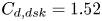 $C_{d,dsk}=1.52$. The droplet deformation is assumed to increase until the initiation of breakup,
 $\tau _b=\tau _{b,i}$, at which point
 $y=1$. Afterwards, we assume that it decreases until
 $t_{b,t}$, when
 $y=0$ again. Droplet deformation increases the transfer of momentum between the gas and particle during this short time, but has only a small effect on the particle velocity equilibration time. Various functions for
 $y(\tau _b)$ are considered in § 5.2. The scalar component of particle drag acceleration,
 $f_D$, is modified from (3.6) for the deformed droplet cross-sectional area
 \begin{equation} f_D = C_d \frac{3}{4}\frac{\rho_{g}d_a^2}{\rho_p d_0^3}v_{pg}. \end{equation}
3.5. Droplet breakup model
For the breakup model, creation of new child droplets, a simple approach was utilised where only the properties of the original Lagrangian point representing the parent droplet(s) are modified. The result is that the number of Lagrangian points is not increased and that we must use a single representative droplet size to describe the distribution of resulting child droplet sizes. For comparison, an alternative approach would have been to create additional points representing different sized child droplets, though even for a simple breakup process of relatively small droplets, this would result in the number of points increasing by a factor of 100 or more. For the cases explored here, this would produce up to 10 million points on the Lagrangian mesh, a number which is beyond our current computational capabilities, but only just. In the future we will pursue a multi-point breakup method, but for now we can learn much from the simpler approach used here.
As discussed in § 3.4, the breakup properties, including the final number of child droplets,  $n_f$, is determined at
 $\tau _b=0$. The predicted final droplet size,
 $d_f$, is calculated based on the properties of the droplet at
 $\tau _b=0$, and used to determine
 $n_f$ by conservation of mass. Various models for
 $d_f$ are presented later in § 5.2. In this way, the initial number of particles per Lagrangian point,
 $n_0$ (parcel size), may be greater than one, and
 $d$ at
 $\tau _{b,t}$ may be decreased by mass transfer as the breakup process progresses, i.e.
 $d(\tau _{b,t}) \le d_f$. The number of particles in the parcel,
 $n$ increases continuously through the breakup process and is not limited to whole numbers. Conceptually, this is not realistic, but it has the effect of providing a smooth process. This prohibits numerical instabilities resulting from sudden increases in mass transfer when
 $n$ jumps to the next whole number. We have found these to pose a problem for high Mach number accelerations, not considered here. The rate of breakup, i.e.
 $n(\tau _b)$, is set by various models described later in § 5.2.
3.6. Simulation domain and initial conditions
The experimental geometry provides a quasi-2-D interface, data are from a centre slice of the interface, thus 2-D simulations are appropriate for comparison. Initial and boundary conditions are set to replicate those of the experiments, while limiting computational time, as shown in figure 4. The shock tube conditions and particle concentrations must be set, such that they fit with the experimental conditions near the interface. With the initial conditions of the shock tube (e.g.  $P_1$,
 $T_1$ and
 $\boldsymbol {v_{g,1}}$) and the 1-D shock-jump relations providing post-shock conditions (e.g.
 $P_2$,
 $T_2$ and
 $\boldsymbol {v_{g,2}}$), the simulation is initiated with a shock wave already developed and in motion, as shown in figure 4. For particle generation, we assumed a distribution (see §§ 4.2 and 5.1) for the size of particles and uniform distribution for their locations. Particles are generated in the circular region shown in figure 4 such that the effective density of the dispersed region provides the Atwood number given from experimental measurements. Our simulation is done in centimetre-gram-second units, resulting in an effective domain depth (third dimension) of 1 cm.
Schematic of the simulation initial conditions and domain.

The gas mesh is generated by dividing the domain with  $2$ blocks in the
 $y$-direction and
 $120$ in the
 $x$-direction. Each block has
 $8\times 8$ zones and the zones are square (equal height and width). The AMR is allowed to refine the mesh up to five times (6 levels total) for the highest resolution studied, zone width
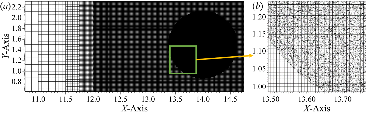
 ${\sim }49\ \mathrm {\mu }$m (see § 4.3). AMR is performed with a moving window that refines the interface completely in the
 $Y$ direction, and from the minimum to maximum
 $X$ location of particles and carrier gas. The shock wave is fully refined before each interaction with the interface (incident shock and reshock). Figure 5 shows five levels of mesh refinement with the particle point location before the incident shock interaction. A magnified region is shown to illustrate how the particle points are randomly located within the interface region.
Gas and particle mesh. (b) Shows a magnified region of particles and the gas mesh.

While the simulation results are provided on a 2-D mesh, a unit depth (1 cm in our case) is considered for calculating the mass of the gas in a zone. The particle point can be thought of as existing in the centre of this 3-D zone, and uniformly applying its effects along the imagined third dimension. For parcels of particles, the particles represented by the point can be thought of as being uniformly distributed in the imagined third dimension. Each particle in the parcel has the same properties (size, temperature, etc.). Thus, the gas field then remains 2-D, while the particles are modelled as 3-D spheres.
4. Evaporation effects
The effects of evaporation are explored using case 1 from Middlebrooks et al. (Reference Middlebrooks, Avgoustopoulos, Black, Allen and McFarland2018). The effects of evaporation are isolated from breakup in this case due to the small droplet sizes (breakup does not occur). A validation of the current evaporation model under shock-driven conditions is presented first. A comparison of simulation and experimental results is then presented, with a discussion on the effects of evaporation on the SDMI following.
4.1. Evaporation model validation
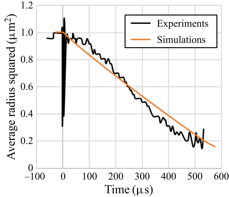
To validate our particle models under shock-driven conditions, we simulated the experimental conditions of Goossens et al. (Reference Goossens, Cleijne, Smolders and van Dongen1988). In this work, a shock/expansion tube is used to first condense water droplets, by means of an expansion wave, which super-cools a nitrogen–water–vapour mixture, inducing droplet growth. This method produces droplets with a highly uniform size of  ${\sim }2\ \mathrm {\mu }$m. A shock wave, with Mach number of 1.572, is then initiated and passes through the gas with droplets. Light extinction measurements are then made at two wavelengths to measure time-dependant droplets sizes. The size measurements are made in a small volume, providing mean droplet size, number density and size distribution. The droplets were shown to decrease in size following the d-squared law.
To simulate this experiment, a reduced size 2-D computational domain ( $0.2\times 25$ cm2) was used, simulating a small portion of the experimental domain (
 $1260\times 10\times 10$ cm3). Since the experimental conditions were one-dimensional (uniform distribution of droplets) with minimal boundary effects, the use of the reduced simulation domain is appropriate, and reduces the computational resources needed. The initial conditions (
 $T_1=275$ K,
 $P_1=65$ kPa and droplet mass fraction of 0.0053) and shock wave Mach number (
 $M=1.572$), for the case presented in figure 6 from Goossens et al. (Reference Goossens, Cleijne, Smolders and van Dongen1988), were matched in the simulation and outflow boundaries were used on all sides to prevent boundary effects. A log normal droplet size distribution, with mean initial droplet diameter of
 $2\ \mathrm {\mu }$m and standard deviation of
 $0.1\ {\rm \mu}{\rm m}$, was used. The average droplet radius was tracked over time in a
 $0.1\times 0.2$ cm2 region of the simulation domain. This measurement was repeated for several different areas of the computational domain, finding similar results, and suggesting that boundary and resolution effects did not alter the results.
Droplet evaporation rates in 1-D shock tube: simulation and experimental data from Goossens et al. (Reference Goossens, Cleijne, Smolders and van Dongen1988).

The data from Goossens et al. (Reference Goossens, Cleijne, Smolders and van Dongen1988) figure 6(c) were digitally extracted and plotted along with our simulation data in figure 6. From this figure, we can see that our evaporation model agrees well, with perhaps a slightly slower evaporation rate. It should be noted that the full breakup and deformation model, described more later, was used, but no breakup occurred due to the small droplet size. It was found that deformation had a negligible effect on the evaporation rate.
4.2. Initial conditions
To isolate the effects of evaporation from breakup, case 1 from Middlebrooks et al. (Reference Middlebrooks, Avgoustopoulos, Black, Allen and McFarland2018) was simulated. The initial conditions selected for the simulation comparison are shown in table 1. The  $A_e$ used in the simulations,
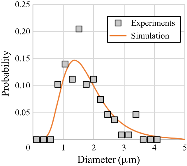
 $A_e=0.06$, as described in § 2.2. A log-normal distribution was fit to the experimental data for droplet sizes (figure 7). The mean droplet diameter is
 $1.8\ \mathrm {\mu }$m with a standard deviation of
 $0.8\ \mathrm {\mu }$m. A cutoff for the maximum,
 $d_{max}=5\ \mathrm {\mu }\mathrm {m}$, and minimum,
 $d_{min}=0.5\ \mathrm {\mu }\mathrm {m}$ particles sizes was used.
Droplet size distribution for case 1.

4.3. Resolution study
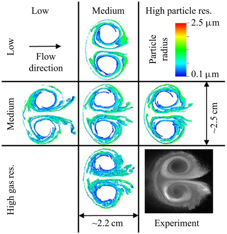
A resolution study was conducted to determine the effect of the gas and particle resolutions. For PIC simulations, both the gas mesh resolution and particle resolution (parcel size or the number of particles represented on a point,  $n_0$) have an effect on the interface evolution. The gas mesh resolution was set by employing additional levels of AMR. The gas mesh resolutions selected were 64, 128 and 256 zones per diameter of the circular interface. Due to the small size of the particles for this case, we did not have the computational resources to simulate the required number of points for
 $n_0<10$. Parcel sizes of 10, 40 and 160 were selected where the multiple of 4 was used to match the effect of increasing the gas mesh resolution in two dimensions.
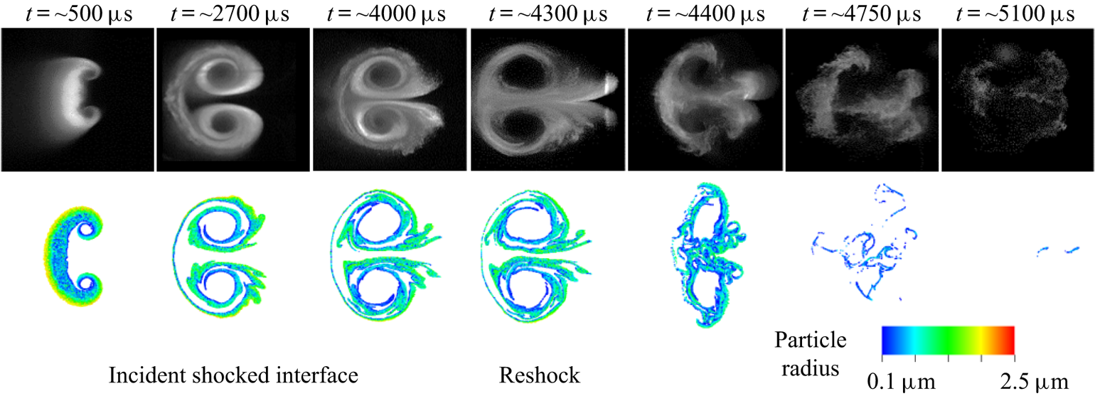
A qualitative comparison of the results was performed at a late time,  $t=4$ ms, where the morphology of the interface had developed, but reshock had not occurred yet. Figure 8 shows the particle field for five different combinations of gas and particle resolutions. Here the particle radii were plotted, and while the relative size of the plotted simulation points was not correlated directly to the Mie-scattered light measured in the experiments, the locations of the points gives some measure of the degree to which the simulations reproduced the morphology of the particle field.
Droplet field at 4 ms for 3 different gas and particle resolutions. An experimental image of the droplet field is provided in the lower right for comparison.

Interestingly, as particle resolution increased, the development of the particle jets, lines of particles extending from the interface to the right, decreased. The converse was true for gas resolution, higher resolution led to more developed jets. The medium gas resolution case was the lowest resolution to show the development of these jets, while the medium particle resolution was able to reproduce some of the spread of these jets. We attribute the thicker layers of particles, and fan-like structures observed in the experiments to 3-D effects (vorticity spreading in the  $Z$, axial, direction).
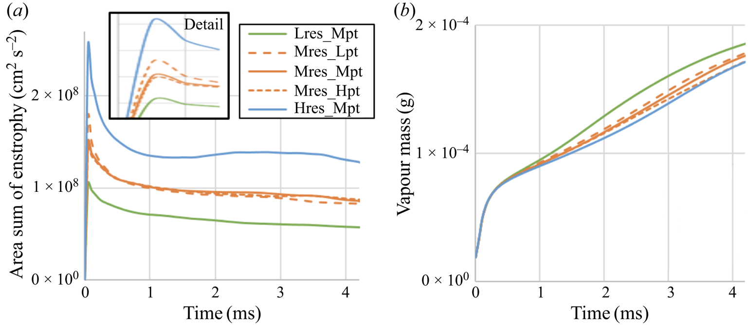
Figure 9 shows that the enstrophy (vortical energy) is not converged for the cases (convergence is not expected until the resolution is comparable to the smaller turbulent length scales), but that the vapor mass is similar for all cases. Given that the focus of this paper in on comparing the morphology of the interface in simulations and experiments, and in exploring the effects of evaporation and breakup on the SDMI, we have chosen to use the medium gas resolution, 128 zones per interface diameter and medium particle resolution,  $n_0=40$.
(a) Area sum of enstrophy over time for different gas and particle resolutions. (b) Vapour mass over time for different gas and particle resolutions.

4.4. Comparison with experiments
Figure 10 shows a time series of experimental images and plots of the simulation particle field. Overall, the simulations are able to match the large-scale morphology of the experiments, as discussed in § 4.3. At early times, the particle layers are thinned in the simulations. This could be a 3-D effect, or an effect of our limited gas mesh resolution. Small-scale structures, below our gas resolution, may be working on the interface in the experiments to produce a more diffuse particle region. The most noticeable difference between the experiments and simulations occurs after reshock, where the simulations show a more rapid evaporation of the droplets. An excessive evaporation rate might also explain some of the discrepancies before reshock, where a lower evaporation rate may allow particles to survive longer in the surrounding dry gas, allowing the formation of the fan-like structure in the particle jets. While the evaporation model was validated for quasi-1-D conditions (§ 4.1) with similar droplet sizes, it seems to show poorer performance for a 2-D case where strong gradients in the vapour concentration exist.
Experimental and simulation images of the droplet field evolution. The experimental images were originally published by Middlebrooks et al. (Reference Middlebrooks, Avgoustopoulos, Black, Allen and McFarland2018).

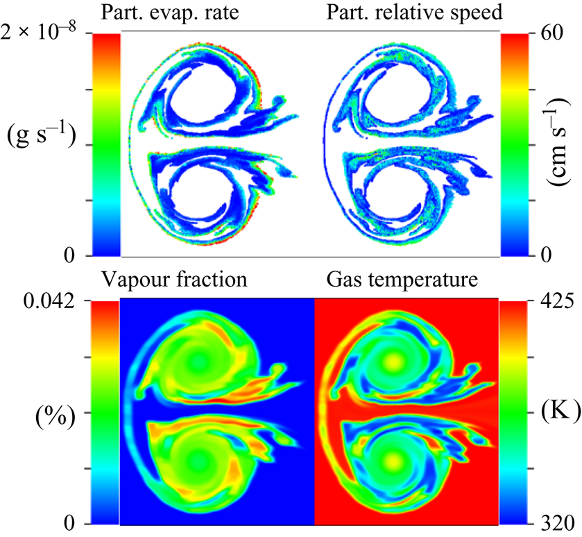
Further insight into the effect of evaporation on the SDMI can be gained from the simulation results. Figure 11 shows several flow field quantities at  $t=4$ ms. From this figure, we can see that droplet evaporation rates are highly non-uniform. Evaporation rates are highest on the outside edge of the interface where the primary vortices create the largest particle relative velocities,
 $v_{pg}$. The vapour fraction in the gas is also highly non-uniform with pockets of high density vapour existing in the jets and near the regions of high droplet evaporation rate. Interestingly, the vapour is pulled into the vortex cores, despite the fact that droplets are never pulled into this region. The gas temperature closely follows the vapour field, and results in a highly perturbed gas density field. This perturbed gas density field is important to the deposition of vorticity during reshock, and may help explain the number of small-to-medium-scale structures seen in the post-reshock experimental droplet field.
Case 1 particle and gas properties at 4 ms.

5. Breakup effects
In this section, the effects of breakup with simultaneous evaporation are explored for case 3 from Middlebrooks et al. (Reference Middlebrooks, Avgoustopoulos, Black, Allen and McFarland2018), where breakup effects are dominant due to larger droplets. Several breakup models were considered first by examining the resulting droplet sizes. The most promising two models were examined further and the best selected and used for an exploration of breakup effects in the SDMI.
5.1. Initial conditions
To explore the effect of droplet breakup, case 3 from Middlebrooks et al. (Reference Middlebrooks, Avgoustopoulos, Black, Allen and McFarland2018) was simulated. As described in § 2.2, the value of  $A_e$ used was 0.021. This was outside of the value reported by Middlebrooks et al. (Reference Middlebrooks, Avgoustopoulos, Black, Allen and McFarland2018) of
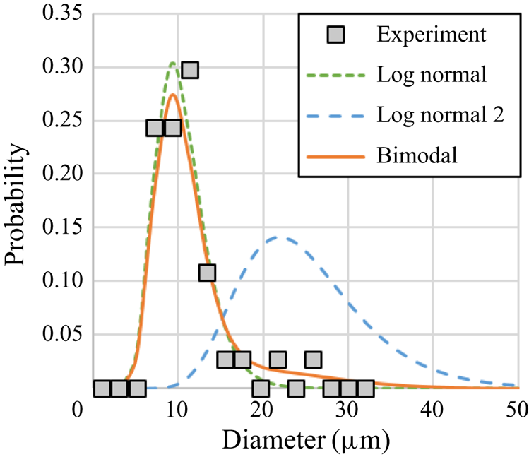
 $0.014 \pm 0.003$, but matched our new measurements and was found to produce vorticity deposition that qualitatively matched the experimental results better. The previous reported droplet size measurements proposed a log-normal distribution for initial droplet sizes. Here we used a bi-modal distribution instead (figure 12). This distribution fit the experimental data better and produced larger particles after breakup, forming the observed trailing particle tail. The bi-modal distribution may be explained by the presence of agglomerated droplets formed in the particle generation apparatus.
Droplet size distribution for case 3.

The bimodal distribution consisted of two log-normal distributions. The first log-normal distribution has a mean droplet diameter of  $10.5\ \mathrm {\mu }$m and a standard deviation of
 $3\ \mathrm {\mu }$m. The second log-normal distribution has a mean droplet diameter of
 $25\ \mathrm {\mu }$m and a standard deviation of
 $7.5\ \mathrm {\mu }$m. Droplet sizes were selected from the first distribution with a 90 % probability, leaving the second distribution to be used for approximately 10 % of the droplet sizes. A cutoff for the maximum droplet size,
 $d_{max}=95\ \mathrm {\mu }$m, was used. The probability density function of the combined bi-model distribution is shown in figure 12 as the solid line.
5.2. Breakup model parameters
In § 3.5 we outlined our breakup methods excluding the selection of exact models for deformation rate, breakup time and predicted child droplet size. Here we present the results for various models to explain the development of our model.
For deformation and breakup, several of the models described in § 1.4 were considered. These models are applicable to our flow conditions as they were developed for shock-driven conditions at low particle volume fractions where particle-to-particle interactions are negligible ( $\epsilon$ is less than 0.01 % for case 3). While these models neglect
 $Ma$,
 $Re$ and thus
 $Kn$ effects, these are expected to be negligible in our case as our initial
 $Kn$ for case 3 is of the order of 0.002, where recent simulation work (Syahdan Reference Syahdan2015) has shown that breakup closely resembles that found in the continuum regime. While the TAB/ETAB model provided a well-tested method for describing the particle deformation prior to breakup, it was found to disagree, on breakup time and child droplet size, with the most relevant data for shock-driven particle breakup (i.e. Hsiang & Faeth Reference Hsiang and Faeth1992). Instead, an empirical data-fitting approach was taken to describe the breakup times and deformation rate. The breakup times were taken from the experimental data of Dai & Faeth (Reference Dai and Faeth2001) (figure 8 in reference), where a power-law equation was fit for
 $\tau _{b,i}$
 \begin{gather} \tau_{b,i} = \min(3,3.328We_\delta^{{-}0.1310}) \end{gather}
and a sixth-order polynomial for  $\tau _{b,t}$
 \begin{gather}\tau_{b,t} = \begin{cases} 3.186\,\mathrm{e-}9We_\delta^6-7.765\,\mathrm{e-}7We_\delta^5+ \\ 7.380\,\mathrm{e-}5We_\delta^4 -3.366\,\mathrm{e-}3We_\delta^3+ & We \le 76.45 \\ 7.002\,\mathrm{e-}2We_\delta^2-0.4158We_\delta+4.798 \\ 6 & We > 76.45 . \end{cases}\end{gather}
where  $We_\delta =We-12$. These data were determined to be the most applicable to our case, and presented the most current addition to the data of Hsiang & Faeth (Reference Hsiang and Faeth1992).
The rate of distortion was found from a curve fit to the experimental data of Chou & Faeth (Reference Chou and Faeth1998) for  $C_d$, i.e. it was assumed that
 $y$ follows the same evolution as the
 $C_d$ reported. Two power-law equations were fit to the data, before and after initiation of breakup
 \begin{equation} y = \begin{cases} (\tau_{b}/\tau_{b,i})^{3.2}, & \tau_b\le \tau_{b,i} \\ \left(1-\dfrac{\tau_b-\tau_{b,i}}{\tau_{b,t}-\tau_{b,i}}\right)^{7.5}, & \tau_{b,t}\ge \tau_b>\tau_{b,i} \\ 0 & \tau_b > \tau_{b,t}. \end{cases}\end{equation}
After the initiation of breakup,  $\tau _b>\tau _{b,i}$, the resulting child droplets and breaking parent droplets are assumed to have a single representative
 $y$ that follows the parent drop
 $C_d$ data. After the breakup process is complete,
 $y$ is reset to 0, and another breakup process may begin. It was found that the rate of distortion and its effect on momentum transfer had little effect on the SDMI development due to the relatively short time for distortion and breakup.
The most significant breakup parameter for our SDMI experiments, was the final child droplet size,  $d_f$. As discussed in § 3.5 we limited our model to a single representative size for all child droplets, the SMD, or
 $d_{32}$. Several models were available (see § 1.4) to predict
 $d_f$. Before implementing these models in our simulation, we examined the resulting droplet sizes for the range of droplet sizes present in our initial size distribution. Figure 13 A shows the
 $d_{32}$ (SMD) ratio,
 $d_f/d_0$, over a range of applicable
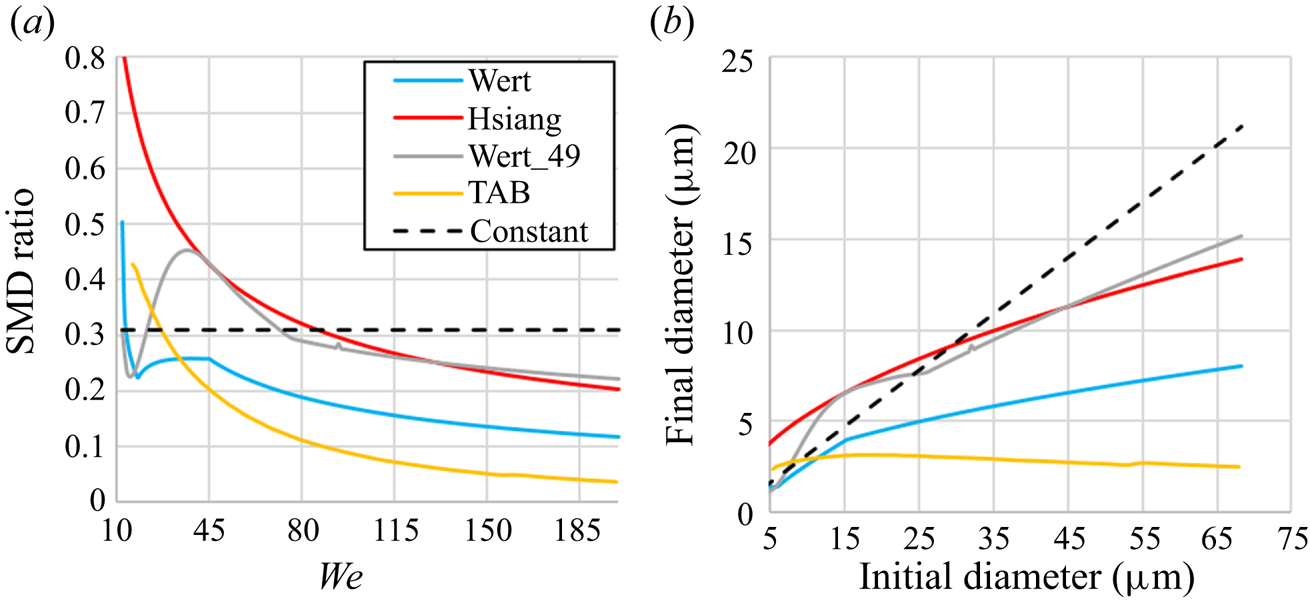
 $We$ for the existing models of Hsiang & Faeth (Reference Hsiang and Faeth1992), labelled Hsiang, Wert (Reference Wert1995), labelled Wert, and O'Rourke & Amsden (Reference O'Rourke and Amsden1987), labelled TAB. Note that these models use their own breakup parameters, i.e. breakup times. Two new models are discussed later, a constant
 $d_{32}$ ratio of 0.31 model and a modified version of the Wert model.
(a) The  $d_{32}$ ratio versus initial droplet Weber number for various breakup models. (b) Final versus initial droplet sizes for various breakup models.

From the droplet lag distance and reshock breakup observed in the case 3 experimental data, we could estimate that the breakup model needed to produce  $10\ \mathrm {\mu }$m or greater droplets from the range of initial sizes (figure 12). Figure 13(b) shows that several of the existing models can be eliminated based on this criteria. The TAB model produces droplets that are much too small as noted in previous work (Tanner Reference Tanner1997). The Wert model is said to perform better at
 $We<100$ (Guildenbecher et al. Reference Guildenbecher, López-Rivera and Sojka2009), but also fails to produce the observed large droplets. While the Hsiang model produced larger droplets at high
 $We$, it over-predicts the size of droplets at low
 $We$, as noted by others (Chou & Faeth Reference Chou and Faeth1998; Guildenbecher et al. Reference Guildenbecher, López-Rivera and Sojka2009).
Two new models were developed in an effort to produce more accurate child droplet sizes. The first of these is the Constant model, a simple model using a constant  $d_{32}$ ratio of 0.31. This value was selected based on the findings of Zhao et al. (Reference Zhao, Liu, Xu, Li and Lin2013) and Chou & Faeth (Reference Chou and Faeth1998) for low
 $We$, below 20, breakup. Extending this to
 $We>80$, predicted much larger
 $d_f$ than observed in any previous experiments. The second model we developed, labelled Wert_49, was a modified version of the Wert model (Wert Reference Wert1995)
 \begin{equation} d_f=0.49(We(\tau_{b,t}-\tau{b,i}))^{2/3}\frac{\sigma}{v_{pg}^2\rho_g}. \end{equation}
The breakup times derived from Dai & Faeth (Reference Dai and Faeth2001) (5.1) and (5.2) were used instead of those from Pilch & Erdman (Reference Pilch and Erdman1987), as used in the original model. The leading coefficient, 0.49 here, was selected such that at low  $We$ the
 $d_{32}$ ratio was similar to that of Chou & Faeth (Reference Chou and Faeth1998) and Zhao et al. (Reference Zhao, Liu, Xu, Li and Lin2013), while approximating the
 $d_{32}$ ratio of the Hsiang model at high
 $We$, as seen in figure 13. Note that the kink in the curve for this model, occurring at
 $We \approx 80$, is a product of the change in the breakup time,
 $\tau _{b,t}$, occurring at
 $We>76.45$ (see (5.2)).
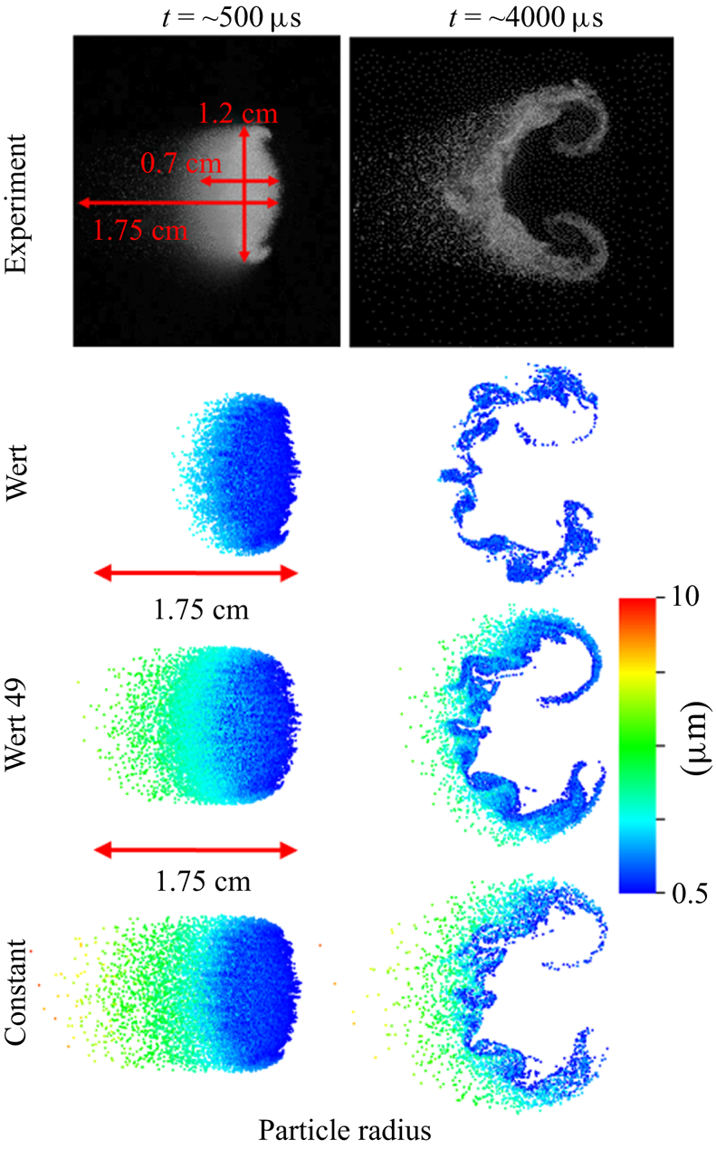
Figure 14 shows the results of the two new breakup models compared with the experiments. For comparison, results from the original Wert model are included. The only quantitative measures of breakup that can be extracted from the existing experiments, are the dimensions of the particle containing region, specifically the trailing particle region (particle tail). All three models show similar development for the primary interface region (dense particle containing region excluding the tail). While the Wert model matches the length of the primary interface, it does not show the formation of the particle tail. Both the Wert_49 and Constant models show this tail region at early time, though, the Constant model shows a tail longer than observed in the experiments. At later time, the Constant model shows persisting droplets in the tail region, while those in the Wert_49 model have mostly evaporated. The morphology and number density of particles in the vortices is more closely matched by the Wert_49 model. The Constant model shows that the layer of particles on the upstream (left) side of the primary interface, is thicker than seen in the experiments. From this evidence, we believe that the Wert_49 model performs better, and that its absence of a strong particle tail at late time is indicative of an over prediction of evaporation, as observed in case 1, or the presence of larger particles in the initial particle size distribution. For now we choose the Wert_49 model for further comparison with the experiments.
Experimental and simulation droplet fields at 0.5 and 4.0 ms for three different breakup models.

5.3. Comparison with experiments
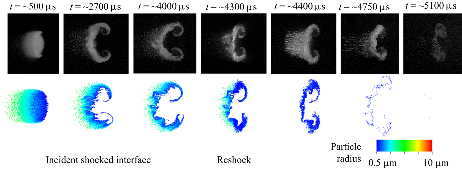
Figure 15 shows the evolution of the interface for both experiments and simulations. The simulations match the overall interface morphology again, but under-predicts the development of the primary vortex cores. This may be an effect of the initial  $A_e$ selected being too small, or due to the over-prediction of child droplet sizes from small, low
 $We$ parent drops. The particle tail appears longer in the simulation at early times, but is missing at late times and after reshock. A possible explanation for this is that the breakup model needs to produce fewer but larger droplets for the particle tail.
Experimental and simulation images of the droplet field evolution. The experimental images were originally published by Middlebrooks et al. (Reference Middlebrooks, Avgoustopoulos, Black, Allen and McFarland2018).

A droplet breakup model that produced a distribution of child sizes may be able to correct both problems (vortex strength and particle tail persistence). A distribution of child droplet sizes formed from each parent drop would produce many smaller droplets, which strengthen and are entrained into the primary vortices, while also producing a small amount of larger child droplets, as observed in the particle tail. In future work, we will explore the effect of child droplet size distributions using a more advanced model that generates additional Lagrangian points to represent a distribution of child droplet sizes.
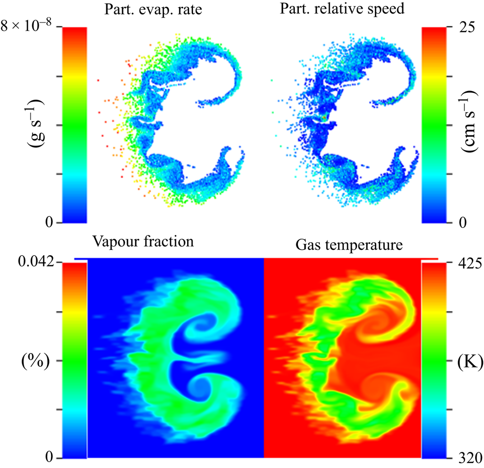
As seen in case 1, the droplets also evaporate faster in the simulation than in the experiments. Figure 16 shows various particle and gas properties relevant to evaporation at late time. Note that the scale for evaporation rate, and for particle relative velocity are different than in figure 11.
Case 3 particle and gas properties at 4 ms.

Similar to case 1, droplet evaporation rates are high on the outside edge of the primary vortices, where relative velocities are high (though, not as high as case 1) and the particles interact with dry gas. Unlike case 1, the droplet evaporation rate is highest (higher than the maximum in case 1) on the upstream side of the interface and in the particle tail, due to the relative isolation of these droplets. This increased evaporation is likely the reason the particle tail is diminished greatly at later times.
The vapour field (same scale as figure 11) shows that there is less vapour present in the interface than in case 1, but given the low  $A_e$ and large particle size, the vapour production is surprisingly large. The morphology is notably different in that there are no high vapour concentration pockets. The droplets in the particle tail have produced some vapour far to the right of the interface not seen in case 1. The gas temperature field also shows higher temperatures than those found in case 1. Both gas fields (temperature and vapour) show a stronger vortex formation than seen in the particle fields. This may indicate that the vortex development is more similar to the experiments, but that the breakup model is not producing droplets that are small enough to be entrained into the vortices.
5.4. Breakup effects on mixing
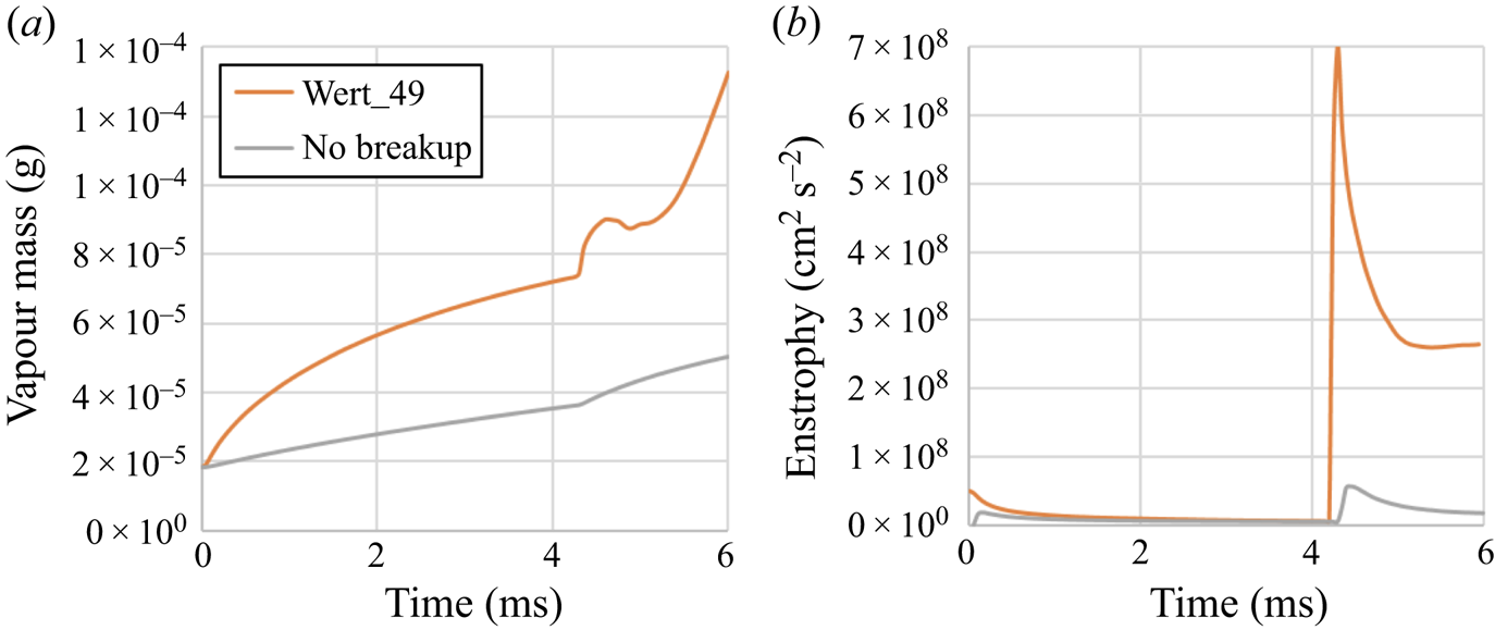
To highlight the importance of breakup in SDMI applications, we have run a simulation of case 3 where breakup is prohibited. The ability to create these non-physical scenarios is an advantage of simulations. The effect of breakup is most apparent in the morphology of the interface, where without breakup the interface does not develop at all, but remains a stretched oval region of particles. Figure 17 A shows the area sum of enstrophy over time with and without breakup. The reduction in droplet sizes from breakup has a substantial impact on vorticity, and the enstrophy deposition is an order of magnitude higher for both the incident shock interaction and the reshock interaction ( $t \sim 4.2$ ms). This energy is responsible for developing the large-scale mixing that cascades down to smaller scales, mixing the droplet and vapour with the surrounding gas.
(a) Case 3 enstrophy over time for the Wert 49 model compared with a case with no breakup. (b) Case 3 vapour mass over time for the Wert 49 model compared with a case with no breakup.

Figure 17(b) shows the production of vapour over time for case 3 with and without breakup. Breakup leads to a rapid increase in vapour production at early times, and a vapour mass that is twice as large before reshock. After reshock this difference increases even more. Clearly, if mixing and vapour production are to be accurately predicted, as is needed in multiphase combustion applications, then breakup must be accurately modelled.
6. Conclusions
The evaporation model has been validated with 1-D experiments and shown to be consistent with the d-squared law. Effects of breakup and deformation were considered in the validation, and were found to be negligible. However, when implemented in a 2-D simulation of the SDMI (case 1 from Middlebrooks et al. Reference Middlebrooks, Avgoustopoulos, Black, Allen and McFarland2018), the evaporation rate was shown to be too high. One possible explanation for this is that non-continuum effects were neglected in our models. While negligible at early times, these effects may become significant as droplets decrease in size (increase in Knudsen number) and may reduce the evaporation rate at late times. Also, high gradients in the vapour mass fraction exist at the edges of the interface where evaporation rates are the highest. These regions are challenging for the existing evaporation model and may be responsible for its poorer performance in SDMI simulations.
Several existing breakup models were tested in simulations of case 3 from Middlebrooks et al. (Reference Middlebrooks, Avgoustopoulos, Black, Allen and McFarland2018), but none produced the wide range of child droplet sizes (particle tail region) observed in the experiments. A new droplet model, based on the Wert model (Wert Reference Wert1995), was developed and implemented in simulations. This model yielded better agreement with other existing experiments over a wide range of  $We$. For an SDMI interface, this model produced development closer in appearance to that of the experiments, showing the formation of a trailing region of large particles (the particle tail region). However, the large particles in the tail region evaporated too rapidly, and there were few smaller particles present to be entrained into the primary vortices. A model producing a distribution of child droplet sizes, as opposed the single representative size (
 $d_{32}$) used by our current model, may correct these issues by allowing for both more smaller droplets, and the formation of some even larger droplets.
Additionally, the hydrodynamic mixing present in SDMI has been shown to have a strong effect on the evaporation rate of the particles. This effect has yet to be captured by current 1-D evaporation models. The SDMI interface morphology has been shown to be highly sensitive to the droplet size distribution, as hydrodynamic mixing has been observed to be inversely proportional to droplet size. As a result, an accurate breakup model with a wide domain of parametric validity will be required to model SDMI and the applications in which it appears.
In our future work we will seek develop a new breakup model, capable of producing an accurate distribution of child droplets sizes. We will also work to include non-continuum effects in our evaporation model as the droplets approach zero radius, and to refine our evaporation model for the high shear, high vapour fraction gradient conditions found in the SDMI. Ultimately, we seek to develop models that capture the combined and concurrent effects of droplet breakup and evaporation.
Acknowledgements
The authors would like to thank the National Science Foundation for their support of this work through award number 1844603 and award number 1812946. The computation for this work was performed on the high performance computing infrastructure administered by Research Computing Support Services at the University of Missouri, Columbia Mo. V.D.-W., W.C.M. and S.R.A. contributed equally to this work.
Declaration of interests
The authors report no conflict of interest.