1 Introduction
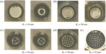
Magnetic liquids – also known as ferrofluids – are stable colloidal suspensions of magnetite particles in carrier liquids, typically synthetic hydrocarbons, esters or water (Rosensweig Reference Rosensweig1997). Ferrofluids are polarizable materials, i.e. they attain magnetization in an external magnetic field. The difference in the magnetization across interfaces between magnetic and non-magnetic media generates force which favours interface distortion in the direction of the applied field and thus it competes against counteracting forces. A case in point is the competition between gravity and surface tension, on one hand, and magnetic force on the other, at the flat free surface of a ferrofluid pool in a vertical magnetic field. As long as the applied field strength remains below a threshold, the flat free surface is stable due to the prevailing action of gravity and surface tension. Beyond the threshold, magnetic force takes over, flatness is overturned and the so-called normal field or Rosensweig instability sets in accompanied by abrupt and pointed free surface deformation – spikes – in the direction of the applied field (Cowley & Rosensweig Reference Cowley and Rosensweig1967). Depending on the experimental conditions, such as pool size and shape, magnetic field strength and its rate of change, or the ferrofluid properties (i.e. magnetic permeability, surface tension), the resulting deformation shape is axisymmetric or two-dimensional with a striking regularity, usually of hexagonal or square symmetry. Samples of the plethora of observed surface deformations are shown in figure 1. In figure 1(a) a single spike is shown at the centre of the pool and in figure 1(b) ring-like patterns are shown; both configurations are axisymmetric. Single spike deformation has a maximum height at the centre of the pool while ring-like patterns have a local minimum at the centre of the pool. In the pools in figure 1(c–e), two-dimensional patterns are favoured. Notice that, although the pools in figures 1(a) and 1(c) are of the same diameter, they favour different surface deformation shapes since they contain ferrofluids of different physical properties, thus patterns of different wavelengths are produced. In all cases, the ferrofluid underneath the free surface remains static and, therefore, the free surface deformation is assumed to follow equilibrium paths if the strength of the applied field is varied quasi-statically.
Free surface deformation of cylindrical magnetic liquid pools. Single spike (a) observed at field strength of 17.8 mT. Ring-like patterns; (b) observed at 14 mT (left) and 16.1 mT (right). Three or 4 spikes (c) observed at 16.7 mT and 17.2 mT respectively. Hexagonal patterns (d) observed at 19.3 mT. Square patterns (e) observed at 18 mT. Notice that at (a)
 $k_{c}=0.533~\text{mm}^{-1}$
while at (b–e)
 $k_{c}=0.616~\text{mm}^{-1}$
;
 $k_{c}=\sqrt{\unicode[STIX]{x1D70C}g/\unicode[STIX]{x1D70E}}$
is the capillary wavenumber,
 $\unicode[STIX]{x1D70C}$
and
 $\unicode[STIX]{x1D70E}$
denote the density and the surface tension of the ferrofluid, respectively.

The normal field instability has been studied both theoretically and experimentally. Competition between hexagonal and square patterns has been investigated in theory (Gailitis Reference Gailitis1977; Friedrichs & Engel Reference Friedrichs and Engel2001) and in experiments (Abou, Wesfreid & Roux Reference Abou, Wesfreid and Roux2000; Gollwitzer, Rehberg & Richter Reference Gollwitzer, Rehberg and Richter2006). Solitary patterns have been discovered in experiments by Richter & Barashenkov (Reference Richter and Barashenkov2005) and studied numerically by Lavrova, Matthies & Tobiska (Reference Lavrova, Matthies and Tobiska2008). Localized hexagonal patterns have been investigated by Lloyd et al. (Reference Lloyd, Gollwitzer, Rehberg and Richter2015). Axisymmetric ring (Knieling et al. Reference Knieling, Richter, Rehberg, Matthies and Lange2007) or single spike (Gollwitzer et al. Reference Gollwitzer, Spyropoulos, Papathanasiou, Boudouvis and Richter2009) patterns have been seen in experiments and studied numerically (Gollwitzer et al. Reference Gollwitzer, Spyropoulos, Papathanasiou, Boudouvis and Richter2009; Lavrova, Polevikov & Tobiska Reference Lavrova, Polevikov and Tobiska2017). A mechanism, for the formation of hexagonal patterns, is proposed by Cao & Ding (Reference Cao and Ding2014) and it is based on numerical computations. However there are still important aspects to be investigated. Most challenging among them is the selection mechanism among the plethora of shapes that are candidates to dominate the free surface at the onset of the instability and beyond. Determining selection among different deformation shapes amounts to determining the stability of any shape with respect to admissible disturbances, which carry symmetries different from that of the shape itself. The experimental evidence suggests that pool size (primarily diameter as well as depth) finiteness causes the formation of incipient patterns at the side walls (Boudouvis Reference Boudouvis1987; Boudouvis et al. Reference Boudouvis, Puchalla, Scriven and Rosensweig1987), which are not to be ignored in determining the generation of and the selection among different surface shapes.
The challenge here is to reveal the underlying mechanism of pattern selection in a small ferrofluid pool where its size allows for the appearance of a single ring-like deformation or (depending on the applied field strength) of only few spikes (2, 3 or 4). In particular the challenge is to answer the following questions: (i) how one-dimensional (ring-like) equilibrium shape families are connected with two-dimensional (2-, 3- or 4-spike) ones and (ii) how two-dimensional shape families can evolve from each other by changing key parameters like the field strength.
Both one- and two-dimensional surface deformations are computed and their stability is determined. The governing equations of capillary magnetohydrostatics along with their boundary conditions account for gravity, surface tension, wetting and variable magnetic permeability of the ferrofluid. They are discretized and solved with the Galerkin/finite element method and Newton iteration, for the magnetic field distribution inside the ferrofluid and in the surrounding air and for the free surface shape. Stability and bifurcation analysis is feasible, by solving standard eigenvalue problems with the Jacobian matrix of the linearized equation sets, since the field distribution and the free surface shape are solved for simultaneously. Such a tedious task is for the first time presented in the context of pattern stability analysis since in previous works (Gollwitzer et al. Reference Gollwitzer, Matthies, Richter, Rehberg and Tobiska2007; Lavrova et al. Reference Lavrova, Matthies and Tobiska2008; Cao & Ding Reference Cao and Ding2014) the field distribution and the free surface were decoupled and thus linear stability analysis was not feasible.
The mathematical formulation is presented and the computational methods employed are outlined in § 2. In § 3 the experimental set-up is outlined and the properties of the ferrofluid are given. The experimental results are presented in § 4. In § 5, the computational results for one- and two-dimensional patterns are presented. Conclusions are given in § 6.
2 Three-dimensional capillary magnetohydrostatics and computational analysis
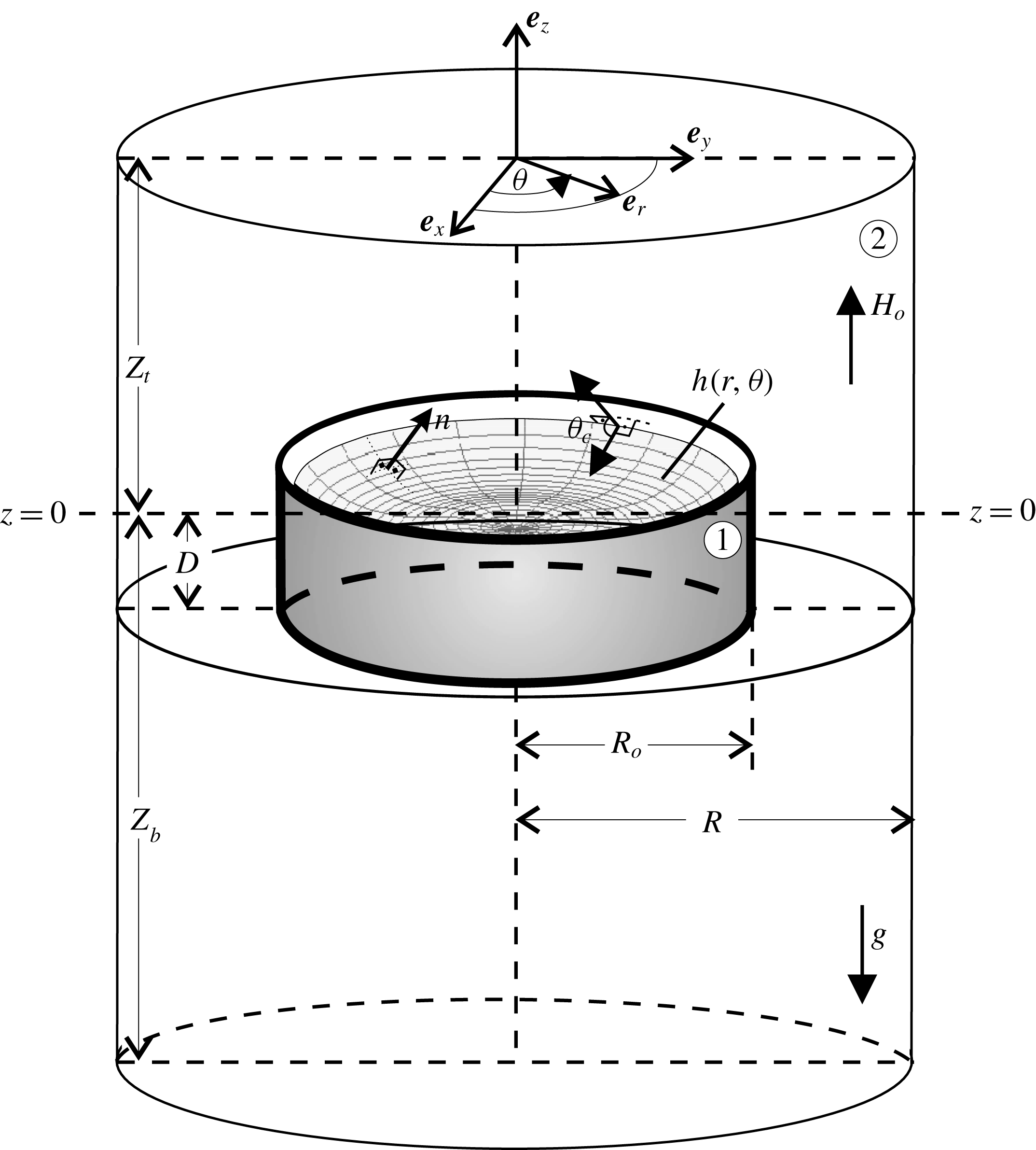
A laterally bounded ferrofluid pool in a magnetic field and surrounded by air is shown in figure 2; the ferrofluid and air are denoted by 1 and 2, respectively. The applied field is static, uniform and vertical, in a region around the pool; such a region could be the inner space of a solenoid. The field uniformity, however, is disturbed in the neighbourhood of the pool, due to the demagnetizing field of the magnetic liquid itself. Therefore, the applied magnetic field could be taken as uniform only away from the pool. The equations governing the magnetohydrostatic equilibrium of the pool are given in detail elsewhere (Rosensweig Reference Rosensweig1997) and they are simply summarized here. The static magnetic field
 $\boldsymbol{H}$
is irrotational and so it can be derived from a magnetostatic potential,
 $u$
, i.e.
 $\boldsymbol{H}\equiv \unicode[STIX]{x1D735}u$
, both inside and outside the ferrofluid. The magnetic induction,
 $\boldsymbol{B}$
, is governed by the Gauss law, i.e.
 $\unicode[STIX]{x1D735}\boldsymbol{\cdot }\boldsymbol{B}=0$
, and, provided that the materials are isotropic, it is parallel to
 $\boldsymbol{H}$
, and so is the magnetization,
 $\boldsymbol{M}$
:
 $$\begin{eqnarray}\boldsymbol{B}=\unicode[STIX]{x1D707}\boldsymbol{H}=\unicode[STIX]{x1D707}_{o}(\boldsymbol{H}+\boldsymbol{M}),\quad \boldsymbol{M}=\unicode[STIX]{x1D712}\boldsymbol{H},\quad \unicode[STIX]{x1D712}\equiv \left(\frac{\unicode[STIX]{x1D707}}{\unicode[STIX]{x1D707}_{o}}-1\right).\end{eqnarray}$$
A laterally bounded cylindrical ferrofluid pool in a vertical magnetic field:
 $R_{o}$
, radius of the pool;
 $D$
, depth of the pool;
 $R$
,
 $Z_{t}$
,
 $Z_{b}$
, distances that mark how far from the pool the magnetic field is uniform.

Therefore, the governing equations for the magnetostatic potential in media 1 and 2 are:
 $$\begin{eqnarray}\unicode[STIX]{x1D735}\boldsymbol{\cdot }(\unicode[STIX]{x1D707}_{1}\unicode[STIX]{x1D735}u_{1})=0,\quad \unicode[STIX]{x1D735}\boldsymbol{\cdot }(\unicode[STIX]{x1D707}_{2}\unicode[STIX]{x1D735}u_{2})=0.\end{eqnarray}$$
The magnetic permeability,
 $\unicode[STIX]{x1D707}$
, and susceptibility,
 $\unicode[STIX]{x1D712}$
, are constant in non-magnetic media, namely
 $\unicode[STIX]{x1D707}_{2}=\unicode[STIX]{x1D707}_{o}=4\unicode[STIX]{x03C0}\times 10^{-7}~\text{H}~\text{m}^{-1}$
,
 $\unicode[STIX]{x1D712}_{2}=0$
. Although in air, equation (2.2) reduces to Laplace’s equation for
 $u_{2}$
, in the ferrofluid it does not, unless,
 $\unicode[STIX]{x1D707}_{1}$
(and thus
 $\unicode[STIX]{x1D712}_{1}$
), are taken to be independent of the field strength.
The latter assumption, although realistic at low field strengths, causes appreciable discrepancies between theoretical predictions and experimental measurements as the field strength increases. Langevin’s theory for monodisperse colloidal suspensions provides the constitutive equation for
 $\unicode[STIX]{x1D707}=\unicode[STIX]{x1D707}(H)$
(Rosensweig Reference Rosensweig1997):
 $$\begin{eqnarray}\frac{\unicode[STIX]{x1D707}_{1}(H)}{\unicode[STIX]{x1D707}_{o}}=1+\frac{3\unicode[STIX]{x1D712}_{i}}{\unicode[STIX]{x1D70F}H}\left(\coth (\unicode[STIX]{x1D70F}H)-\frac{1}{\unicode[STIX]{x1D70F}H}\right),\end{eqnarray}$$
where
 $\unicode[STIX]{x1D712}_{i}$
, called the initial susceptibility, is the susceptibility at low applied field strength and
 $\unicode[STIX]{x1D70F}$
is computed from measurement of the magnetization at saturation,
 $M_{s}$
.
Force balancing along the free surface yields the magnetically augmented Young–Laplace equation of capillarity:
 $$\begin{eqnarray}-g\unicode[STIX]{x1D6FF}\unicode[STIX]{x1D70C}z+\frac{1}{2}\unicode[STIX]{x1D707}_{o}\unicode[STIX]{x1D712}_{1}^{2}(\boldsymbol{n}\boldsymbol{\cdot }\unicode[STIX]{x1D735}u_{1})^{2}+\int _{0}^{H_{1}}M_{1}(H^{\prime })\,\text{d}H^{\prime }+\unicode[STIX]{x1D70E}C=K,\quad z=h(r,\unicode[STIX]{x1D703}),\,0\leqslant r\leqslant R_{o},\end{eqnarray}$$
where
 $z$
is the vertical distance of a point at the free surface from a reference level and
 $K$
is a reference pressure, constant along the free surface;
 $g$
is the gravitational acceleration,
 $\unicode[STIX]{x1D6FF}\unicode[STIX]{x1D70C}$
the difference between the ferrofluid and air densities and
 $\unicode[STIX]{x1D70E}$
the surface tension. The free surface location is defined in cylindrical coordinates,
 $h=h(r,\unicode[STIX]{x1D703})$
. The unit normal to and the local mean curvature of the free surface are, respectively:
 $$\begin{eqnarray}\displaystyle & \displaystyle \boldsymbol{n}=\frac{-h_{r}\boldsymbol{e}_{r}-(h_{\unicode[STIX]{x1D703}}/r)\boldsymbol{e}_{\unicode[STIX]{x1D703}}+\boldsymbol{e}_{z}}{\sqrt{1+h_{r}^{2}+(h_{\unicode[STIX]{x1D703}}/r)^{2}}}, & \displaystyle\end{eqnarray}$$
 $$\begin{eqnarray}\displaystyle & C\equiv 2\aleph =-\unicode[STIX]{x1D735}_{s}\boldsymbol{\cdot }\boldsymbol{n}, & \displaystyle\end{eqnarray}$$
 $\boldsymbol{e}_{r}$
,
 $\boldsymbol{e}_{\unicode[STIX]{x1D703}}$
,
 $\boldsymbol{e}_{z}$
are unit vectors in the
 $r$
,
 $\unicode[STIX]{x1D703}$
and
 $z$
directions,
 $h_{r}\equiv \unicode[STIX]{x2202}h/\unicode[STIX]{x2202}r$
,
 $h_{\unicode[STIX]{x1D703}}\equiv \unicode[STIX]{x2202}h/\unicode[STIX]{x2202}\unicode[STIX]{x1D703}$
,
 $\unicode[STIX]{x1D735}_{s}\boldsymbol{\cdot }(\,)$
denotes the surface divergence operator.
The reference pressure,
 $K$
, in (2.4) is determined by an integral constraint, which imposes the liquid incompressibility
 $$\begin{eqnarray}\int _{0}^{2\unicode[STIX]{x03C0}}\int _{0}^{R_{o}}hr\,\text{d}r\,\text{d}\unicode[STIX]{x1D703}=0.\end{eqnarray}$$
The boundary conditions on the governing equations are (see also figure 2):
 $$\begin{eqnarray}u_{1}=u_{2},\quad \unicode[STIX]{x1D707}_{1}\boldsymbol{n}\boldsymbol{\cdot }\unicode[STIX]{x1D735}u_{1}=\unicode[STIX]{x1D707}_{2}\boldsymbol{n}\boldsymbol{\cdot }\unicode[STIX]{x1D735}u_{2}\quad \text{at}~z=h(r,\unicode[STIX]{x1D703})~\text{and}~0\leqslant r\leqslant R_{o}\end{eqnarray}$$
 $$\begin{eqnarray}u_{1}=u_{2},\quad \unicode[STIX]{x1D707}_{1}u_{1r}=\unicode[STIX]{x1D707}_{2}u_{2r}\quad \text{at}~r=R_{o}~\text{and}~-D\leqslant z\leqslant h(R_{o},\unicode[STIX]{x1D703})\end{eqnarray}$$
 $$\begin{eqnarray}u_{1}=u_{2},\quad \unicode[STIX]{x1D707}_{1}u_{1z}=\unicode[STIX]{x1D707}_{2}u_{2z}\quad \text{at}~z=-D~\text{and}~0\leqslant r\leqslant R_{o}\end{eqnarray}$$
 $$\begin{eqnarray}u_{2}=0\quad \text{at}~z=-Z_{b}\end{eqnarray}$$
 $$\begin{eqnarray}u_{2z}=H_{o}=B_{o}/\unicode[STIX]{x1D707}_{o}\quad \text{at}~z=Z_{t},\quad u_{2r}=0\quad \text{at}~r=R\end{eqnarray}$$
 $$\begin{eqnarray}\frac{h_{r}}{\sqrt{1+h_{r}^{2}+(h_{\unicode[STIX]{x1D703}}/r)^{2}}}=\cos \unicode[STIX]{x1D703}_{c}\quad \text{at}~r=R_{o}.\end{eqnarray}$$
The subscripts
 $r$
,
 $\unicode[STIX]{x1D703}$
and
 $z$
denote differentiation with respect to
 $r$
,
 $\unicode[STIX]{x1D703}$
and
 $z$
, respectively. Equations (2.7)–(2.9) are statements of the continuity of the potential and of the normal component of the magnetic induction across the interfaces between two media with different magnetic permeabilities. The depth,
 $D$
, of the pool is the average depth, since even at zero applied field the free surface is not flat due to side wall wetting;
 $D$
is calculated by dividing the volume of the ferrofluid in the pool by the cross-section of the pool. A datum for the potential is set by (2.10). Equations (2.11) are the conditions that the magnetic field be uniform far away from the pool. The wetting properties of the liquid at the contact with solid pool walls are accounted through Young’s contact angle,
 $\unicode[STIX]{x1D703}_{c}$
in (2.12). The governing equations are solved for the unknowns
 $u_{1}$
,
 $u_{2}$
,
 $h(r,\unicode[STIX]{x1D703})$
and
 $K$
. The equations give rise to a three-dimensional, nonlinear and free boundary problem because both axisymmetric and non-axisymmetric shapes are sought, which are unknown a priori and must be solved for along with the magnetostatic potential. The equations are discretized by Galerkin’s method of weighted residuals and finite element basis functions. The application of the method will only be outlined here; the details can be found in a previous work (Papathanasiou & Boudouvis Reference Papathanasiou and Boudouvis1998). The governing equations are reduced with Galerkin’s method to a set of nonlinear algebraic equations for the values of the unknowns,
 $u$
and
 $h$
at the nodes and for the value of
 $K$
and solved with Newton iteration. At each step of the Newton iteration, the sparse linearized equation set is solved iteratively by the restarted GMRES(m) method (Saad & Schultz Reference Saad and Schultz1986) preconditioned by a deflation technique (Erhel, Burrage & Pohl Reference Erhel, Burrage and Pohl1996). The multiplicity and stability of solutions at different values of the parameters are computed by computer-implemented bifurcation theory (Keller Reference Keller and Rabinowitz1977).
A parameter of interest here is the strength of the applied magnetic field,
 $H_{o}$
, which appears in the boundary conditions (cf. (2.11)) and the diameter of the pool
 $R_{o}$
(figure 2). Solution branches, i.e. solutions at sequences of different values of
 $H_{o}$
, are systematically traced with first-order continuation. Arclength-type continuation and branch-switching techniques are employed when turning point singularities need to be circumnavigated and bifurcating solution branches need to be followed, respectively. Moreover, the parameter continuation in the solution space includes the search for bifurcation points along the solution branches traced in the continuation process. Near singularities, one or more eigenvalues of the Jacobian matrix, of the linearized equation set, change sign on passing through zero. A simple means of singularity detection is to monitor the smallest-in-magnitude eigenvalues of the Jacobian. However this amounts to solving eigenvalue problems during the entire continuation process. Monitoring the condition number or computing the eigenvalues (Spyropoulos, Palyvos & Boudouvis Reference Spyropoulos, Palyvos and Boudouvis2004; Pashos et al.
Reference Pashos, Kavousanakis, Spyropoulos, Palyvos and Boudouvis2009) of appropriate small scale matrices involved in the GMRES method significantly reduces the costly eigenvalue computations. Thus, these costly computations are only performed at bifurcation points to obtain the eigenvectors needed to compute the bifurcating branches and to determine their stability. When eigenvalue computations are needed, a standard eigenvalue problem is solved with the Jacobian and the 10 smallest in magnitude eigenvalues (monitored eigenvalues) are computed with the ARPACK package (Lehoucq, Sorensen & Yang Reference Lehoucq, Sorensen and Yang1998).
3 Experimental set-up
The ferrofluid, APG J10 (Lot F112200A), from Ferrotec is used for all experiments. The ferrofluid container is placed in a long solenoid, which generates a uniform and vertical magnetic field. The solenoid is 33 cm long with an internal diameter of 13 cm and an external diameter of 14 cm. It has 1124 windings and produces up to
 $2.1~\text{mT}~\text{A}^{-1}$
at its centre, with a variation of less than 1 % at the experimental region. Its inductance is 75 mH. The solenoid is fed by a controllable but constant current power supply. The basic experimental set-up is equipped with 3 Hall sensors for measuring the intensity of both the axial and transverse magnetic fields. The surface of the magnetic fluid in the container is traced by a CCD (charge-coupled device) camera connected to a computer via a USB plug.
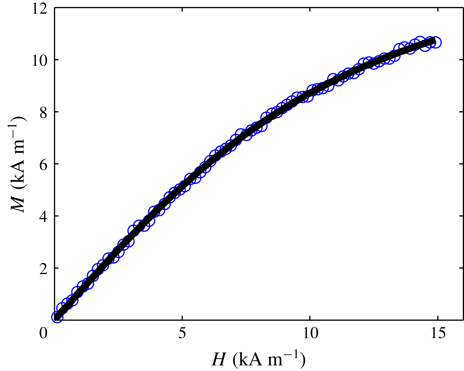
Magnetization curve of the ferrofluid. The blue circles denote the experimental data. The solid line is the fit of the Langevin equation to the initial range (up to
 $H\leqslant 15~\text{kA}~\text{m}^{-1}$
) of the experimental data. The magnetization curve was measured by using an AC magnetometer (see the Appendix).

The APG J10 properties, are the following:
 $\unicode[STIX]{x1D6FF}\unicode[STIX]{x1D70C}=1160~\text{kg}~\text{m}^{-3}$
,
 $\unicode[STIX]{x1D70E}=0.03~\text{N}~\text{m}^{-1}$
,
 $\unicode[STIX]{x1D703}_{c}=10^{\circ }$
,
 $\unicode[STIX]{x1D712}_{i}=1.1$
and
 $M_{s}=19.9~\text{kA}~\text{m}^{-1}$
. The density was measured with a portable density meter and the surface tension with a du Noüy tensiometer. The values of
 $\unicode[STIX]{x1D712}_{i}$
and
 $M_{s}$
were given by Ferrotec. Because the ferrofluid is polydisperse, that is, it consists of magnetic particles with a broad size distribution, the Langevin equation (2.3), used in our computations, cannot describe the whole magnetization curve. Thus, a different value (
 $M_{s}^{\ast }=15.7~\text{kA}~\text{m}^{-1}$
) for the saturation magnetization is used in computations, instead of
 $19.9~\text{kA}~\text{m}^{-1}$
, in order to fit the Langevin equation to the initial range of the magnetization curve (figure 3). The value of
 $M_{s}^{\ast }$
is obtained by the following process: (i) the magnetization curve is fitted to the magnetization part of (2.3) and (ii) according to this fit,
 $\unicode[STIX]{x1D70F}=0.21~\text{m}~\text{kA}^{-1}$
in (2.3) and
 $M_{s}^{\ast }=3\unicode[STIX]{x1D712}_{i}/\unicode[STIX]{x1D70F}$
. The reader is referred to Gollwitzer et al. (Reference Gollwitzer, Spyropoulos, Papathanasiou, Boudouvis and Richter2009) for a computational comparison with Langevin’s equation and a model for polydisperse magnetic fluids by Ivanov & Kuznetsova (Reference Ivanov and Kuznetsova2001). Notice that the value
 $\unicode[STIX]{x1D712}_{i}=1.1$
is close enough to the value
 $\unicode[STIX]{x1D712}_{i}=1.088$
which can be fitted from the measurements shown in figure 3. From the magnetization curve and the properties of the ferrofluid the theoretical critical value of the field strength (Boudouvis Reference Boudouvis1987, equation (5.25)) is found to be
 $B_{c,\infty }=17.0$
mT; this value refers to a laterally unbounded pool.
4 Experimental results
The ferrofluid is placed in a cylindrical glass container of radius
 $R_{o}=18$
mm. The depth is
 $D=10$
mm. Before the onset of instability an axisymmetric deformation (ring-like) is observed, shown in figure 4(a). Past the onset of the instability, the axisymmetric deformation gives way to deformations of 2, 3 or 4 spikes, shown in figures 4(b), 4(c) and 4(d), respectively. By slowly (
 $0.1~\text{mT}~\text{s}^{-1}$
) increasing the applied field strength results in a deformation of 2 spikes, while an abrupt (stepwise) increase favours 3 spikes (
 $0~\text{mT}\rightarrow 16.7~\text{mT}$
) or 4 spikes (
 $0~\text{mT}\rightarrow 17.4~\text{mT}$
) deformation.
By slowly (
 $0.1~\text{mT}~\text{s}^{-1}$
) decreasing the field strength, the 4-spike deformation subsides first, and then transforms into a 2-spike deformation at a critical field. Further decrease of the field strength results in the collapse of the two spikes and the formation of a ring-like deformation. The latter transition sequence is affected by the pool depth. For deeper liquid pools, the experiment showed that 3 of the 4 spikes remain by slowly decreasing the field strength. Further decrease results in 2 spikes which in turn develops to a ring-like deformation.
Free surface deformations in a cylindrical magnetic liquid pool with radius
 $R_{o}=18$
mm and depth
 $D=10$
mm. Before the onset of instability a single ring (a) is observed. At the onset of instability and beyond 2 spikes (b), 3 spikes (c) and 4 spikes (d) are observed.

Therefore the 2-spike deformation is selected either by slowly increasing the field past the onset of the instability, or by slowly decreasing the field in a multi-spike (3- or 4-spike) configuration. Further increase of the field strength changes only the height of the spikes without causing any shape transition. We have observed that only an abrupt (stepwise) increase of the field strength at a high value overtakes somehow the 2-spike deformation and leads to 3- or 4-spike deformation.
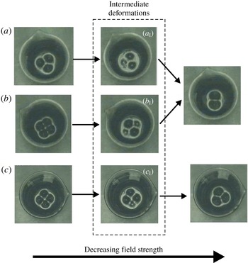
Once formed, the 3-spike deformation is stable to a slow decrease of the field strength down to another critical value of field strength and at that point, 2-spike shapes appear as shown in figure 5. The deformation sequence during the transition from 3 to 2 spikes is shown in figure 5(a). In the case of a 4-spike deformation, by decreasing the field strength, 2- or 3-spike deformations appear as shown in figures 5(b) and 5(c), respectively. The observed sequence of shape transitions, shown in figure 5, is very sensitive to the variation speed and step size of the applied field strength. Practically, in our experimental set-up, the intermediate deformations, namely the ones of figure 5(
 $a_{\text{I}}\text{,}b_{\text{I}}\text{,}c_{\text{I}}$
), cannot be sustained even if the field is kept constant. The shape transitions in figure 5 take place through a continuously decreasing height size of one spike (figure 5
 $a_{\text{I}}$
, figure 5
 $c_{\text{I}}$
) or two spikes (figure 5
 $b_{\text{I}}$
) with practically constant applied field strength.
Free surface shape transition from 3 to 2 spikes (a); from 4 to 2 spikes (b); and from 4 to 3 spikes (c):
 $R_{o}=18$
mm,
 $D=10$
mm in (a,b),
 $R_{o}=18$
mm,
 $D=15$
mm in (c).

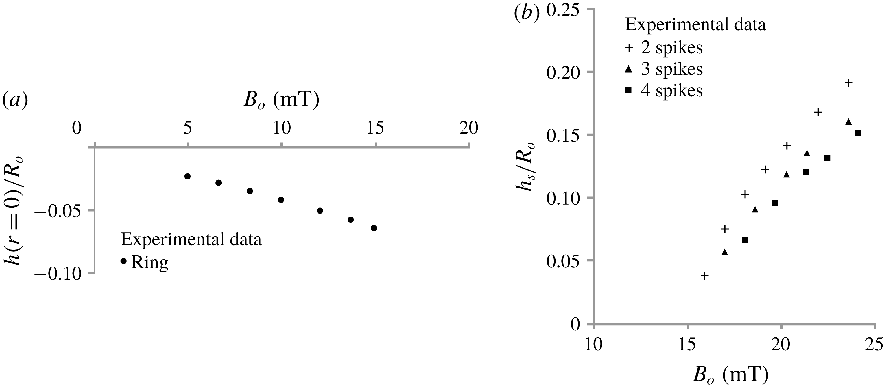
Experimental measurements of the dimensionless height (
 $h(r=0)/R_{o}$
) before the onset of instability (a) and of the spike dimensionless height (
 $h_{s}/R_{o}$
) past the onset of instability (b), versus the applied field strength (
 $B_{o}$
). The radius of the container is
 $R_{o}=18$
mm. The reference level (zero value of the vertical axis) is at a distance
 $D=10$
mm from the bottom of the container. The measurements were performed for increasing
 $B_{o}$
. In the case of the ring-like deformation (a) the measurements were taken at the centre of the pool. In each developed pattern (2-, 3- or 4-spike) all the spikes are of the same height; this height is the one presented here (b).

Figure 6 shows the experimental measurements of the free surface deformation versus the applied field strength
 $B_{o}$
, in a range of
 $0<B_{o}<25$
mT;
 $B_{o}$
is measured above the container at a vertical distance of 32.4 mm from the ferrofluid free surface. This distance is also used in computations – i.e.
 $Z_{t}=32.4$
mm in (2.11). The heights
 $h(r=0)$
and
 $h_{s}$
are measured from the averaged level of the ferrofluid surface as in our mathematical model. The instrument used to measure the surface deformation is based on a laser method and has been presented in our previous work (Megalios et al.
Reference Megalios, Kapsalis, Paschalidis, Papathanasiou and Boudouvis2005). The accuracy of the surface deformation measurement with the laser method depends on the strength of the laser beam reflected back from the free surface. The maximum strength is measured when the surface is locally flat, i.e. at the deformation extrema. Thus the full surface profile cannot be measured with accuracy. Moreover, the accuracy of the proposed method depends on the spike sharpness. Repeated measurements showed good reproducibility with a maximum absolute variation less than 0.25 mm observed for spikes 3 mm in height (i.e. for
 $h/R_{o}=3/18=0.167$
). In Gollwitzer et al. (Reference Gollwitzer, Spyropoulos, Papathanasiou, Boudouvis and Richter2009) this method is compared with an X-ray method developed by Richter & Bläsing (Reference Richter and Bläsing2001).
The free surface falls at the centre of the pool while it climbs at the side walls as long as the field strength does not exceed a critical value. In experiments, the onset of the instability can be deduced from the significant change of the ferrofluid surface deformation. At a value of
 $B_{cr,exp}=15.8$
mT a 2-spike deformation occurs. Before this critical value (about 0.2 mT) a single ring-like deformation is observed in experiments. In this case, the measurements (figure 6
a) were taken at the centre of the pool.
Past the onset of instability the height of the spikes (
 $h_{s}$
), shown in (figure 6
b), corresponds to the maximum vertical displacement of the free surface within a circular ring of
 $0.2R_{o}<r<0.5R_{o}$
. Experimental measurements show that in each developed pattern (2-, 3- or 4-spike) all the spikes are of the same height and as the number of spikes increases their height decreases. It is worth mentioning that the radial position of the spike, i.e. the radial position of the surface maximum is not fixed as the magnetic field varies, even for spikes of the same shape family (solution family in our computations) but can be within a certain range of
 $r$
; that is, the spikes move within the circular ring area as the field increases.
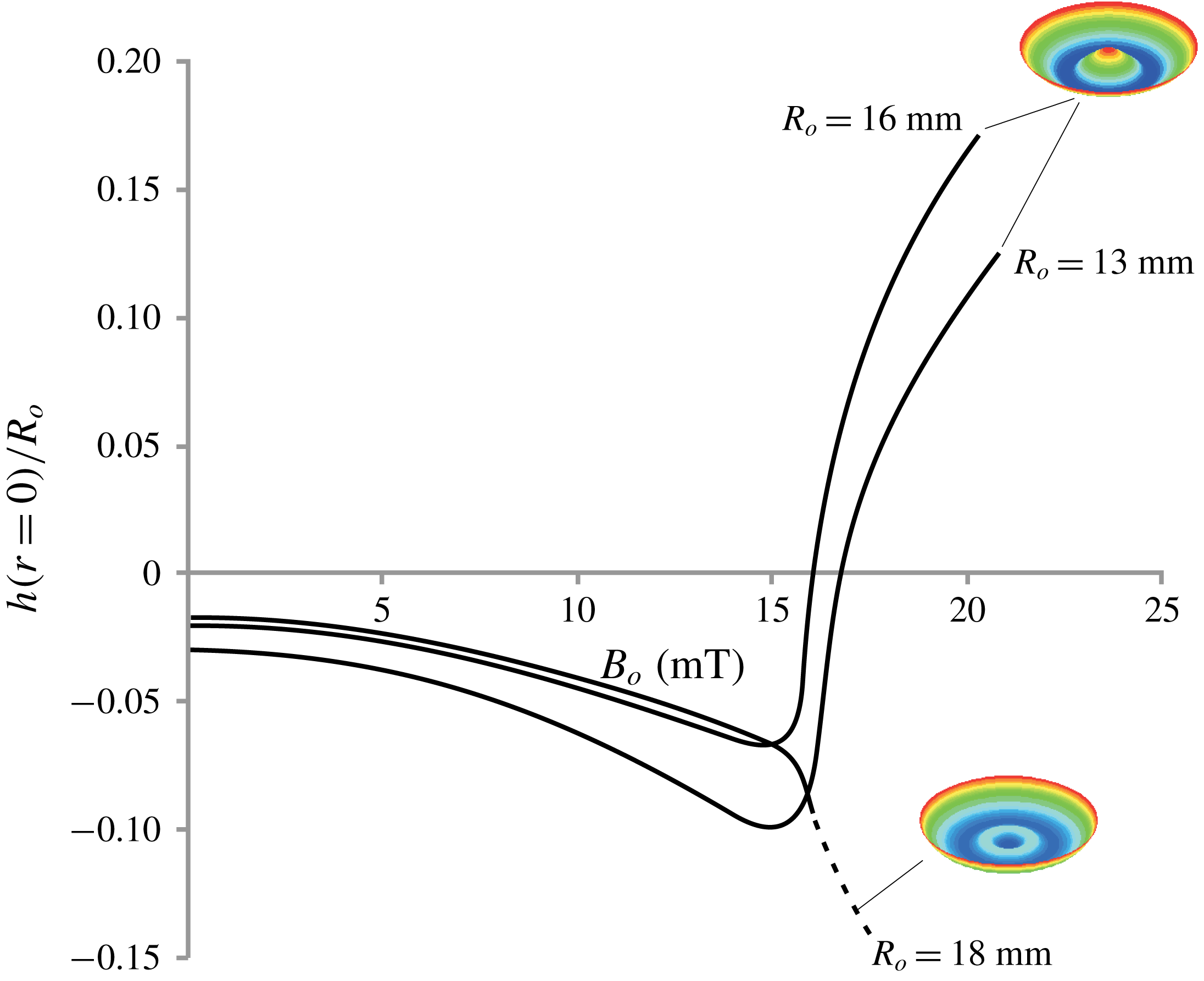
Computational results of the axisymmetric free surface deformation (single spike for the cases of
 $R_{o}=13$
mm and
 $R_{o}=16$
mm and single ring-like deformation for
 $R_{o}=18$
mm) versus the applied field strength
 $B_{o}$
. The reference level (zero value of the vertical axis) is at a distance
 $D=10$
mm from the bottom of the container. The dimensionless height,
 $h(r=0)/R_{o}$
, of the free surface is plotted at the centre of the pool. The insets show computed sample developed patterns. Blue, green and red represent, respectively, the minimum, medium and maximum values.

5 Computational results
5.1 Axisymmetric free surface deformations
The radius of the container is selected by trial such that the only axisymmetric pattern, observed in experiments as well as in computations, was a single ring-like deformation instead of a single spike at the centre of the pool. Figure 7 shows axisymmetric solutions versus the applied field strength
 $B_{o}$
(cf. (2.11)) for different container sizes. Our experiments suggest that 2-, 3- or 4-spike deformations can be accommodated only in containers where the axisymmetric pattern forming is a ring (as in the container with
 $R_{o}=18$
mm in figure 7) and not a single spike (as in the containers with
 $R_{o}=13$
mm or 16 mm in figure 7). This is also verified by our computations where no bifurcation points are detected during the continuation process along the solution branches that correspond to single spike deformations. Notice that the solution branch, that corresponds to the container with
 $R_{o}=18$
mm, after 16.2 mT is marked as unstable (dashed line) which is explained in the next subsection.
5.2 From axisymmetric to non-axisymmetric free surface deformations
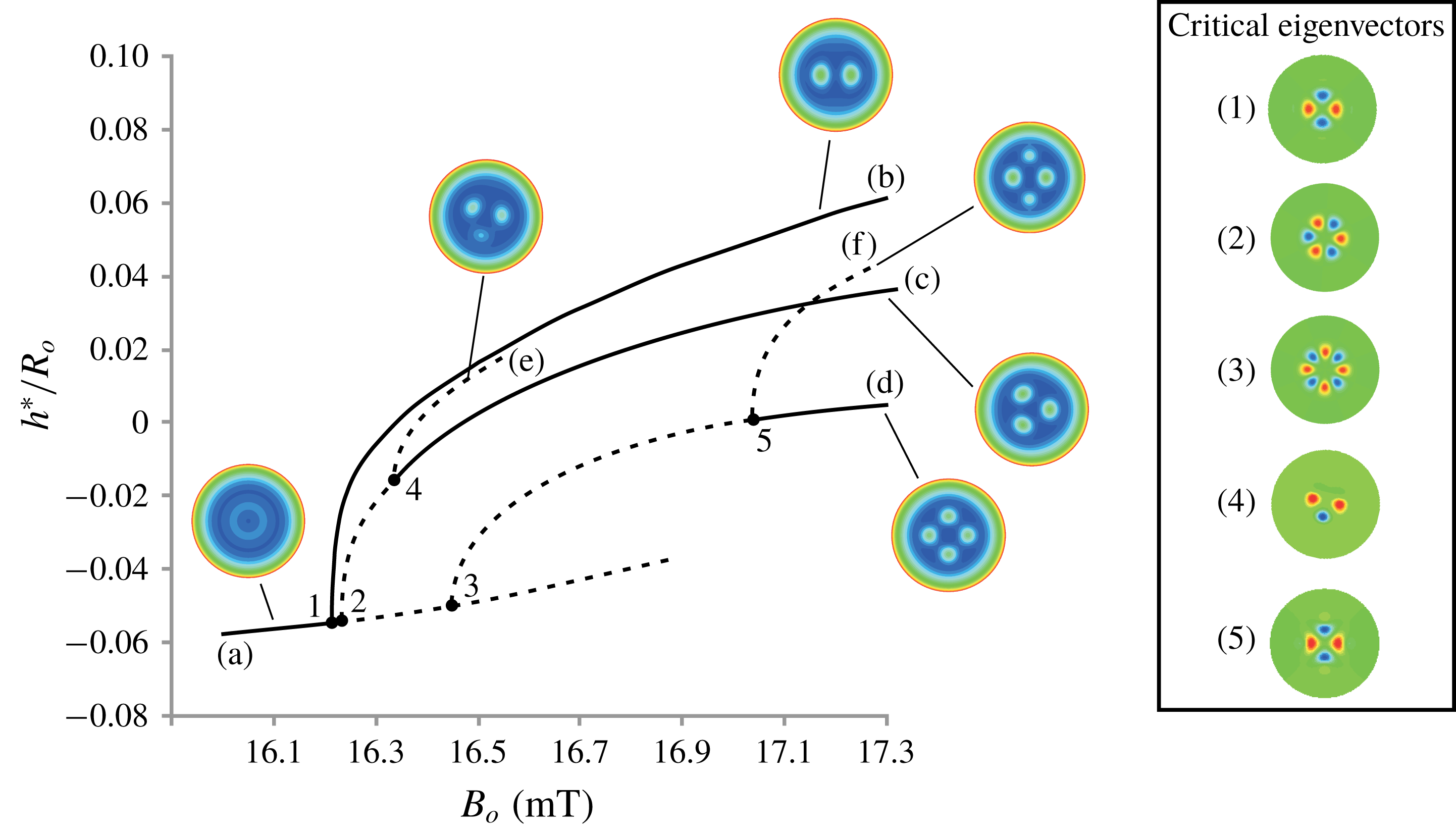
Computational results of the free surface deformation. The dimensionless height,
 $h^{\ast }/R_{o}$
, of the free surface is plotted at
 $r=0.275R_{o}$
and
 $\unicode[STIX]{x1D703}=0$
. The reference level (zero value of the vertical axis) is at a distance
 $D=10$
mm from the bottom of the container. Solid lines denote stable solutions and dashed lines label unstable solutions. The insets on the right-hand side show the critical eigenvectors that correspond to the eigenvalues passing through zero (from a negative to a positive value) at bifurcation points 1, 2, 3, 4 and 5, respectively. The insets that point to the solution branches, (a), (b), (c), (d), (e) and (f), show computed sample developed patterns. Blue, green and red represent, respectively, the minimum, medium and maximum values. The primary instability (bifurcation point 1) is computed at 16.2 mT or at
 $0.95B_{c,\infty }$
. This figure is best viewed in the coloured electronic version of the paper.

Figure 8 shows the computational results in a container of radius
 $R_{o}=18$
mm and depth
 $D=10$
mm. The dimensionless height,
 $h^{\ast }/R_{o}$
, of the free surface at
 $r=0.275R_{o}$
and
 $\unicode[STIX]{x1D703}=0$
is plotted for all branches. The radial position of the maximum deformation of the ring-like pattern is at
 $r=0.275R_{o}$
. Bifurcation points are marked with 1, 2, 3, 4 and 5. Solid lines denote stable solutions (the monitored eigenvalues of the Jacobian matrix are negative) and dashed lines label unstable solutions (one or more eigenvalues are positive). The critical eigenvectors, shown in figure 8, are the critical disturbances that cause changes in the stability of the solution branches and these critical eigenvectors are used to compute the bifurcating branches. The bifurcations are symmetric i.e. pitchfork bifurcations. For the clarity of the presentation only the upper parts of the bifurcating branches are plotted, since the lower branches correspond to solutions that are invariant if rotated by a certain angle.
Three non-axisymmetric branches (b), (c) and (d) bifurcate close to each other from the axisymmetric branch (a). At 16.2 mT (bifurcation point 1 in figure 8) the stable branch (b) bifurcates from the branch (a). The eigenvector (critical eigenvector) that corresponds to the eigenvalue that is passing through zero (from a negative to a positive value) when increasing
 $B_{o}$
at the bifurcation point 1 is shown in figure 8(1). That is, the ring deformation becomes unstable to 2-spike disturbances. Branch (b) is marked as stable as implied by the associated supercritical bifurcation (Strogatz Reference Strogatz2015) at point 1; this is confirmed by parameter continuation on branch (b) along which the monitored eigenvalues are negative. Passing through bifurcation point 2 form left to right, another eigenvalue changes sign (negative to positive) and the corresponding eigenvector is shown in figure 8(2). The bifurcating branch (c) is unstable from bifurcation point 2 to bifurcation point 4. The critical eigenvector at bifurcation point 3 is shown in figure 8(3) and the bifurcating branch (d) is unstable from bifurcation point 3 to bifurcation point 5.
5.3 ‘Jumps’ among surface deformations with different symmetry
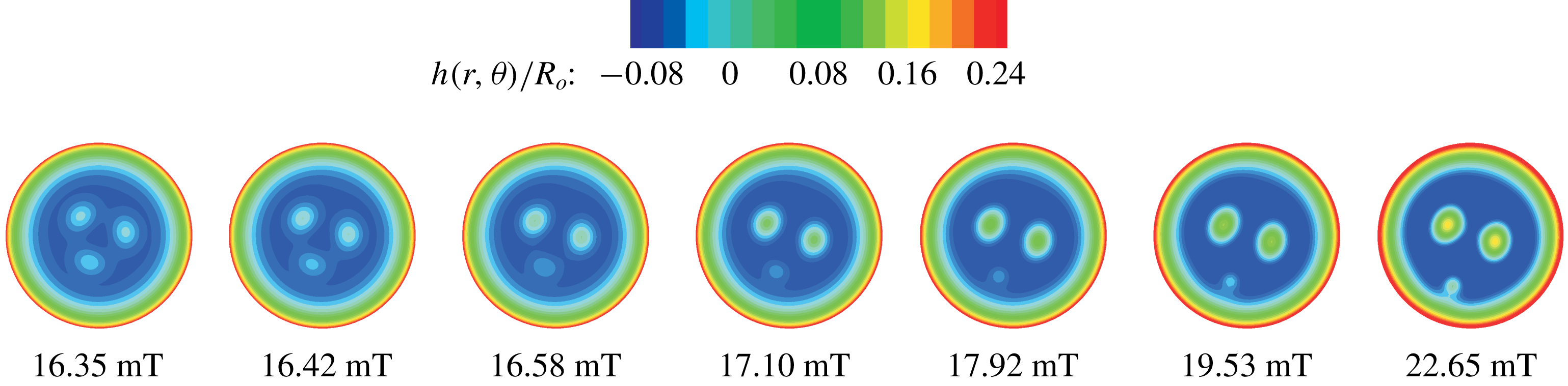
In figure 8, along the branch (c), a new bifurcation point, at 16.35 mT, is detected and marked with 4. Similarly along branch (d), a new bifurcation point, 5, is found at 17.02 mT. The new families are shown in figure 8 and marked with (e) and (f) respectively. The branches (e) and (f) correspond to unstable solutions and their connectivity with the branches (c) and (d) limit the range of stable solutions along them. Along the branch (e), one of the 3 spikes becomes smaller and along the branch (f), two of the 4 spikes subside and this is verified by the symmetry of the critical eigenvectors (the ones with the smallest eigenvalue) computed at the corresponding bifurcation points as shown in figures 8(4) and 8(5). A main 2-spike sub-pattern is developed (cf. insets pointing to branches (e) and (f)) during the parameter continuation, by increasing
 $B_{o}$
, on these branches. Moreover the spikes that are getting smaller are at the same time moving away from the main 2-spike sub-pattern until they ‘stick’ at the side walls. Figure 9 shows a sequence of free surface deformations at selected points on branch (e). Thus, branch (e) eventually approaches asymptotically branch (b), while branch (f) crosses branch (c) (but no bifurcation point is detected) and approaches asymptotically branch (b). The asymptotic convergence of branches (e) and (f) to the branch (b) is speculated since no bifurcation is detected in the parameter range examined. Based on recent computations by Lloyd et al. (Reference Lloyd, Gollwitzer, Rehberg and Richter2015), a snaking scenario for branches (e) and (f) could be revealed in our computations, that is both branches (e) and (f) could be terminated on branch (b). But, as shown in figure 9, the presence of the side walls does not allow the development of the entire pattern. In the absence of or far enough from the side wall a snaking scenario could be uncovered; further investigation in this direction includes parametric analysis with regard to the radius of the pool.
Free surface deformations versus the applied field strength (
 $B_{o}$
) computed during parameter continuation by increasing
 $B_{o}$
, on branch (e) (figure 8).

Free surface deformation versus the applied field strength (
 $B_{o}$
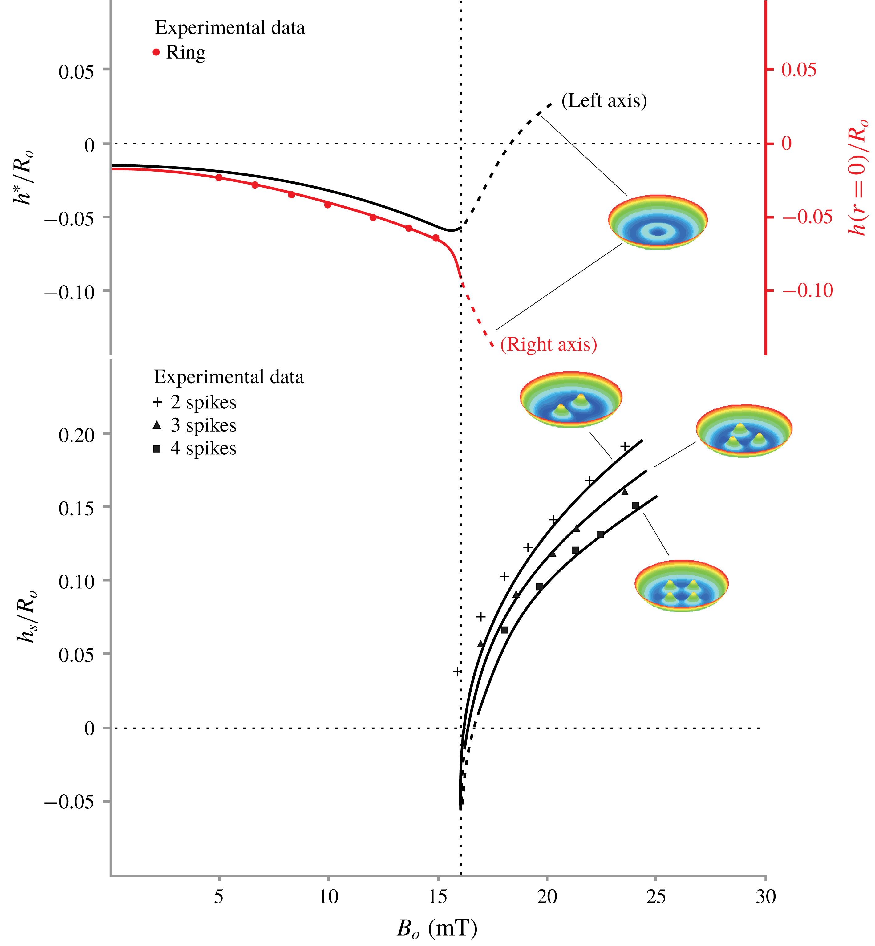
). Comparison between the experimental measurements (symbols) and the computational predictions (lines). The reference level (zero value of the vertical axes) is at a distance
 $D=10$
mm from the bottom of the container. The primary instability (bifurcation point 1 in figure 8) is indicated by the vertical dashed line. The dimensionless height,
 $h(r=0)/R_{o}$
, of the free surface is plotted at the centre of the pool. The dimensionless height,
 $h^{\ast }/R_{o}$
is plotted at
 $r=0.275R_{o}$
and
 $\unicode[STIX]{x1D703}=0$
. The spikes dimensionless height (
 $h_{s}/R_{o}$
) is the maximum vertical displacement of the free surface within a circular ring of
 $0.2R_{o}<r<0.5R_{o}$
. This figure is better seen in the coloured electronic version of the paper.

From figure 8, it is clear that different solutions of different symmetries are not interconnected by any stable solution branch except for the interconnection between the axisymmetric and 2-spike solution branches. Thus the mechanism of selection among surface deformations with a different symmetry can be deduced by paying special attention in the bifurcation points 5 and 4 and the corresponding bifurcating branches in figure 8. Indeed, by slowly decreasing the field strength, 4-spike shapes are stable down to the bifurcation point 5. At the corresponding field strength, only 2-spike or 3-spike shapes are stable. At that point, 2-spike shapes appear in experiments. In computations the critical eigenvector (5), in figure 8, is the critical disturbance that tends to eliminate 2 spikes from the 4-spike shape. At bifurcation point 4 (transition from 3-spike shapes to 2-spike shapes) the critical eigenvector (4), in figure 8, is the critical disturbance that tends to eliminate one spike from the 3-spike shape. Moreover, the transition from 3-spike shapes to 2-spike shapes, by decreasing the field strength, can be explained from the unstable parts of the branches (a), (c) and (d), in figure 8. By slowly decreasing the field strength, 3-spike shapes are stable down to the bifurcation point 4, corresponding to a field strength where only 2-spike shapes are stable. This configuration is then selected since it is the only stable solution and this is observed in experiments, as well.
Experimental measurements (cf. figure 6) compare well with the computational predictions, as shown in figure 10. For the axisymmetric case (ring-like pattern) we also plot an additional branch that corresponds to the axisymmetric branch (a) shown in figure 8. The deviation, that is noticed at the onset of the instability (around of 16 mT), is due to the sensitivity of the spikes height to even small changes of the applied field strength. Notice that, at about 16 mT, all solution families seem to meet because of the drawing scale.
6 Conclusions
In this work, the equilibrium and stability of the free surface shapes of a small size ferrofluid pool in a magnetic field was studied, via bifurcation analysis, to reveal the formation and competition of 2-, 3- and 4-spike deformations. Theoretical predictions were drawn from the equations of capillary magnetohydrostatics by means of the Galerkin/finite element method, Newton iteration, parameter continuation and eigenvalue computations. Computations and experiments show, for the first time, that all non-axisymmetric solutions (2-, 3- or 4-spike shapes) bifurcate form the axisymmetric solution (ring-like deformation). Moreover, eigenvalue computations reveal the mechanism of the transition from 4- or 3-spike shapes to 2-spike shapes. The predicted shapes, the onset of instability and the vertical displacement of the spikes compare well with the experiments.
Acknowledgements
N. Kapsalis and S. Damilos helped with the experiments. We are thankful to Professor E. Hristoforou (NTUA) for providing the instruments for the ferrofluid magnetization measurements. We are also thankful to the referees for valuable comments and suggestions.
Appendix
The magnetization curve, shown in figure 3, was measured by using a race-track tube arrangement with magnetization coil at the one side and search coil at the other one. A peristaltic pump was used to circulate the ferrofluid inside the race-track tube. A wave generator (Agilent 220A) was used to feed a power amplifier (KEPCO BOP 100-4D), to produce a sinusoidal signal from 0.1 Hz up to 10 Hz with current amplitude from 0.1 A up to 30 A. The signal output was fed to a PXI system (NI PXI 6251), serving digital phase lock-in and corresponding detection of the permeability or susceptibility of the sample under test. Theoretical calculations of Ampere’s law have been correlated with calibrated nickel bars, resulting in an uncertainty of the transmitted field of the order of
 ${<}0.1\,\%$
. The arrangement was able to magnetize with a field of up to
 $40~\text{kA}~\text{m}^{-1}$
for 30 min with a temperature increase of
 $3\,^{\circ }\text{C}$
.