I. INTRODUCTION
This paper deals with the comparison of two (solid-state) matched noise sources characterized by their excess noise ratio ENR0. The proposed procedure is simple enough for a non-specialized lab engineer to reach transfer accuracies below 0.1 dB using standard measurement equipment. The procedure can be used:
(1) to check the consistency of two calibrated noise sources;
(2) to verify their evolution over time; and
(3) to calibrate one of the noise sources if the ENR0 of the other is renowned to be accurate.
II. THE CLASSICAL COMPARISON/CALIBRATION FORMULA
The comparison/calibration of two noise sources is basically a double noise temperature measurement of a (theoretically) arbitrary receiver, first with source no. 1 (we will call the reference) and then with source no. 2 (we will call the unknown). The setup for this kind of measurement is described in details in Section V, with Fig. 5 visualizing the symbols used.
Let: T n = receiver noise temperature;
T ron = reference source temperature in its on state;
T xon = unknown source temperature in its on state;
T p = physical (ambient) temperature.
For solid-state noise sources the off temperatures T rof and T xof are supposed to be equal to the ambient temperature T p. The ratio y r of the available noise powers at the receiver output with the reference source on and off then writes [Reference Pozar1]:
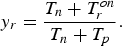 $$y_r=\displaystyle{{T_n+T_r^{on} } \over {T_n+T_p }}.$$
Similarly, with the unknown source, we have:
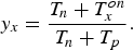 $$y_x=\displaystyle{{T_n+T_x^{on} } \over {T_n+T_p }}.$$
By eliminating the receiver noise temperature T n between (1) and (2), it follows that [2]:
 $$T_x^{on} - T_p=\left({\displaystyle{{y_x - 1} \over {y_r - 1}}} \right)\lpar T_r^{on} - T_p \rpar .$$
Accordingly, the on temperature of the unknown source T xon can be computed from the measured y-factors y r and y x, the on temperature of the reference source T ron and the physical or ambient temperature T p that are supposed to be known.
The conventional excess noise ratio of the newly calibrated source is [Reference Pozar1]:
 $$ENR0_x=10\log \left({\displaystyle{{T_x^{on} - T_0 } \over {T_0 }}} \right)\comma$$
with T 0 = 290 K.
Formula (3) involves two assumptions that are only approximately true:
The receiver noise temperature T n is the same during all four steps of the measurement (with reference source on, reference source off, unknown source on, and unknown source off). This is not perfectly true because the source impedance changes with the device and its state and the receiver noise temperature is a function of this impedance.
The receiver available power gain is the same during all four steps. This is not perfectly true for the same reasons and the fact that the receiver available power gain is a function of the source impedance.
In the experimental part of this work, we will show that errors up to 0.4 dB typically follow because the above assumptions are imperfectly fulfilled. This is much more than for example the instrumentation error of modern noise figure meters, making impedance related errors the most important error cause when comparing noise sources.
III. AN IMPROVED CALIBRATION FORMULA
It is possible to overcome these problems if a receiver with an isolator in front of it is used. With an isolator indeed the noise temperature and the available power gain are closely related (this property is true for all passive devices, the corresponding formula being given in the Appendix). Thanks to it, the errors introduced by the source impedance variations can be eliminated almost completely in a simple way. As shown in the Appendix, formula (3) only has to be modified by a g a factor:
 $$T_x^{on} - T_p=g_a \left({\displaystyle{{y_x - 1} \over {y_r - 1}}} \right)\lpar T_r^{on} - T_p \rpar \comma$$
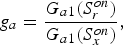 $$g_a=\displaystyle{{G_{a1} \lpar S_r^{on} \rpar } \over {G_{a1} \lpar S_x^{on} \rpar }}\comma$$
where G a1 (S ron) is the available power gain of the isolator connected to the reference source in its on state and G a1 (S xon) is the same with the unknown source.
Computing the g a factor is a simple matter as:
(1) the S-parameters of the isolator are easily measured on a vector network analyzer (VNA);
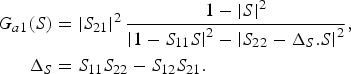
(2) the available power gain G a depends on the source reflection factor S by [Reference Pozar1]:
(7) $$\eqalign{G_{a1} \lpar S\rpar & =\left\vert {S_{21} } \right\vert ^2 \displaystyle{{1 - \left\vert S \right\vert ^2 } \over {\left\vert {1 - S_{11} S} \right\vert ^2 - \left\vert {S_{22} - \Delta _S .S} \right\vert ^2 }}\comma \; \cr \Delta _S & =S_{11} S_{22} - S_{12} S_{21} .}$$
IV. MEASURING THE S-PARAMETERS
A) The setup
All S-parameters were measured using an HP 8722C VNA and a Maury Microwave 8050M TOSL PC 3.5 calibration kit with sliding load. The reason why a sliding load is recommended will appear later.
B) The reflection factors of the noise sources
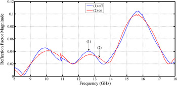
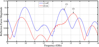
The noise sources are a Micronetics NS346AK (ENR0 ≈ 16 dB) that is used as the reference source and a Micronetics NS346C (ENR0 ≈ 16 dB) that is used as the unknown source. Their reflection factors in both states are shown in Figs 1 and 2. The first source has a stronger internal attenuator that reduces the reflection factor differences between the on and off states. With the second source these differences are much larger and can significantly affect the calibration accuracy.
The reflection factor of the reference source versus frequency. As this source has a 6 dB nominal ENR0 (higher internal attenuator), the reflection factor differences between the on and off states are very small.

The reflection factor of the unknown source versus frequency. As this source has a 16 dB nominal ENR0 (lower internal attenuator), the reflection factor differences between the on and off states are much larger.

C) The S-parameters of the isolator
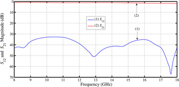
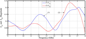
The isolator is a DiTom D418018 dual junction unit with typically 40 dB isolation. Its S-parameters are shown in Figs 3 and 4 and indicate what performance is desirable.
The forward and reverse transmission factors of the isolator.

The reflection factors of the isolator.

V. THE NOISE MEASUREMENTS
A) The setup
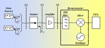
The setup is presented in Fig. 5.
The measurement setup.

The noise sources and the isolator were already defined. The amplifier is a Miteq AFS5-08001800 low-noise device with about 35 dB gain and less than 2 dB noise figure. The SSB downconverter is a custom design with YIG preselector, fundamental mixing and frequency control by an external locking counter. The NFA is an Agilent N8973A instrument. To closely follow all frequency related variations, 401 points are made in the conventional 8–18 GHz band. The noise sources, isolator, and amplifier are all broadband devices with a smooth noise and gain behavior versus frequency. Moreover, the lowest frequency is 8 GHz. So it seemed possible to use the largest bandwidth available on the NFA (4 MHz). To further reduce the random errors, all y-factor measurements were performed with an averaging factor of 16.
B) Comparing the noise sources in different ways
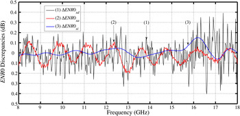
The noise setup can be used as a receiver in three ways by connecting the noise sources at the downconverter input, the amplifier input or the isolator input. We performed y-factor measurements with both sources at all three inputs. For the reference ENR0, we chose the calibration data by the manufacturer at every integer frequency in GHz and linear interpolation between these points. Based on the classical formula (3), an excess noise ratio can be computed in all three cases. They are called ENR0xd (downconverter input), ENR0xa (amplifier input), and ENR0xi (isolator input). The improved formula (5) of course only applies to the isolator input and leads to ENR0xic (isolator corrected). We now compare the set of results based on the classical formula to the results from the improved formula by considering the differences:
 $$\Delta ENR0_{xd}=ENR0_{xd} - ENR0_{xic}\comma$$
 $$\Delta ENR0_{xa}=ENR0_{xa} - ENR0_{xic}\comma$$
 $$\Delta ENR0_{xi}=ENR0_{xi} - ENR0_{xic} .$$
They are plotted versus frequency in Fig. 6. The highest spread (up to ≈ 0.4 dB) occurs on the ENR0xd derived from the measurements at the downconverter input (plane 3 in Fig. 5). This is the input port with the poorest match and the highest noise temperature due to switches, the YIG filter and mixer. Also note the quick variation with frequency that follows from the fact the downconverter is an electrically long device in the 8–18 GHz band. Clearly better (spread below 0.2 dB) are the measurements at the amplifier input (plane 2 in Fig. 5) that has a closer match and a lower noise temperature. A step further is to use the measurements at the isolator input (plane 1 in Fig. 5) that differ from the corrected measurements by 0.15 dB at most. This legitimates the recommendation made in [3] to use isolators as a first stage when calibrating noise sources.
The discrepancies between the ENR0 evaluations.

Now the question arises what is the residual error when using the correction. Provided the isolator has a reverse transfer that is low enough, the associated error mainly depends on how accurately the correction can be computed. This subject is discussed in the next section.
VI. ABOUT THE CORRECTION ACCURACY
From formulas (3) and (5) it follows that the only difference between the classical and improved formula is the ratio g a. Replacing the available power gain by its expression (7) and considering that for the isolator S 12 is very small, we get:
 $$g_a \approx \displaystyle{{1 - \left\vert {S_r^{on} } \right\vert ^2 } \over {1 - \left\vert {S_x^{on} } \right\vert ^2 }}\left\vert {1+S_{11} \lpar S_r^{on} - S_x^{on} \rpar } \right\vert ^2 .$$
So the correction factor mainly depends on the source reflection factors S ron and S xon and the isolator input S-parameter S 11. Let us assume that all reflection factors are affected by a vector error:
 $$\Delta S=\Delta s\, e^{i\phi } .$$
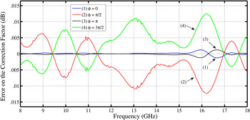
We think that Δs = 0.01 is representative for the directivity error of a VNA calibrated by a sliding load, which is the dominant error when measuring small reflection factors [4]. To see the influence on the ENR0 of such an error, we compute ENR xic with all S-parameters modified by ΔS for φ = 0, π/2, π, and 3π/2. The differences between these ENR xic (with modified S-parameters) and the values with the “true” S-parameters are plotted versus frequency in Fig. 7. They show that the uncertainty on the correction factor is always much smaller than the correction itself.
If state-of-the-art S-parameter measurements are performed, the error on the correction (<0.015 dB) is expected to be much smaller than the correction itself (up to 0.15 dB).

As a consequence, it can be assumed that the impedance related error on the ENR0 measurement of a noise source has been reduced from several tenths of a dB to several hundreds of a dB. At this level, the error becomes of the same order or smaller than the other errors occurring when two sources are compared (instrumentation y-factor error, random y-factor error, drift error of the setup, connector reproducibility error, receiver linearity error, physical temperature error inside the sources and isolator, etc.)
VII. CONCLUSION
Without caution, impedance-related errors are often the dominant contribution to the uncertainty when comparing two noise sources. Thanks to the use of an isolator combined with the correction formula presented in this paper, these errors can on the contrary be reduced to a level where they become negligible. Moreover, the formula is very simple and rests on easy measurements, namely the S-parameters of an isolator. There is no need to define a noise model for the receiver or to measure its input reflection factor, which is much more delicate.
APPENDIX
DERIVATION OF THE IMPROVED CALIBRATION FORMULA
The improved calibration formula (5) only applies to the special case of solid-state noise sources but in theory it is equivalent to the radiometer correction procedures in use at NIST or NPL [Reference Williams5–Reference Randa10]. Moreover, it can be derived rather easily through concepts that are very common in noise theory such as noise temperature, y-factor, available power gain, and cascaded two-ports.
The exact expressions of the y-factors
In its on state the reference source has a reflection factor S ron and an available noise power in a bandwidth Δf given by:
 $$kT_r^{on} \Delta f\comma$$
where k designates Boltzmann's constant.
Hereafter, the receiver is described as a cascade of two two-ports, the first being the isolator and the second being the rest of the chain. Subscript 1 corresponds to the isolator and subscript 2 to the rest of the chain. The subscript 12 stands for the whole receiver. If the receiver has an available power gain G a12 (S ron) and a noise temperature T n12 (S ron), the available output power is:
 $$G_{a12} \lpar S_r^{on} \rpar k\lpar T_r^{on}+T_{n12} \lpar S_r^{on} \rpar \rpar \Delta f.$$
In the off state, this power becomes:
 $$G_{a12} \lpar S_r^{of} \rpar k\lpar T_p+T_{n12} \lpar S_r^{of} \rpar \rpar \Delta f.$$
From (6) and (7), it follows that the y-factor writes:
 $$y_r=\displaystyle{{G_{a12} \lpar S_r^{on} \rpar } \over {G_{a12} \lpar S_r^{of} \rpar }}\displaystyle{{T_r^{on}+T_{n12} \lpar S_r^{on} \rpar } \over {T_p+T_{n12} \lpar S_r^{of} \rpar }}.$$
Similarly, for the unknown source, replacing the r subscripts by x, we get:
 $$y_x=\displaystyle{{G_{a12} \lpar S_x^{on} \rpar } \over {G_{a12} \lpar S_x^{of} \rpar }}\displaystyle{{T_x^{on}+T_{n12} \lpar S_x^{on} \rpar } \over {T_p+T_{n12} \lpar S_x^{of} \rpar }}.$$
The receiver noise temperature and gain
Using the Friis formula for the noise temperature of cascaded two-ports [Reference Pozar1], the overall noise temperature T n12 is:
 $$T_{n12} \lpar S\rpar =T_{n1} \lpar S\rpar +\displaystyle{{T_{n2} \lpar S_{o1} \lpar S\rpar \rpar } \over {G_{a1} \lpar S\rpar }}.$$
In this relation S designates the source reflection factor and S o1 the first stage output reflection factor, which is a function of the source reflection factor S given by [Reference Pozar1]:
 $$S_{o1} \lpar S\rpar =S_{22}+\displaystyle{{S_{12} S_{21} } \over {1 - S_{11} S}}S\comma$$
where the S ij are the first stage (isolator) S-parameters.
The isolator is a linear passive device at physical temperature T p. Accordingly, the following relation holds between its noise temperature T n1 and its available power gain G a1 [Reference Pozar1]:
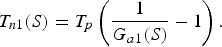 $$T_{n1} \lpar S\rpar =T_p \left({\displaystyle{1 \over {G_{a1} \lpar S\rpar }} - 1} \right).$$
Moreover, the available power gain G a12 of the cascade is the product of the available power gains of the first and second stages G a1 and G a2 provided they are computed for the right reflection factors:
 $$G_{a12} \lpar S\rpar =G_{a1} \lpar S\rpar G_{a2} \lpar S_{o1} \lpar S\rpar \rpar .$$
We now introduce a fundamental assumption which is of course an approximation but a much better approximation than simply assuming the overall noise temperature and available power gain do not depend on the source impedance. For an isolator (especially a two-stage design) the reverse transfer S 12 is very small (in the experiments it was typically −35 dB or less). It then follows from equation (11) that the dependence of S o1 on S is very small. As a consequence, S o1 can be considered the same for all source reflection factors S ron, S rof, S xon, and S xof and both T n2(S o1(S)) and G a2(S o1(S)) can be replaced by the constant values T n20 and G n20.
The overall result
Putting the expressions (10), (12), and (13) in (8) and (9) and making the above assumptions leads to:
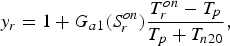 $$y_r=1+G_{a1} \lpar S_r^{on} \rpar \displaystyle{{T_r^{on} - T_p } \over {T_p+T_{n20} }}\comma$$
 $$y_x=1+G_{a1} \lpar S_x^{on} \rpar \displaystyle{{T_x^{on} - T_p } \over {T_p+T_{n20} }}\comma$$
Eliminating T n20 between (14) and (15) produces the improved calibration formula:
 $$T_x^{on} - T_p=\left({\displaystyle{{G_{a1} \lpar S_r^{on} \rpar } \over {G_{a1} \lpar S_x^{on} \rpar }}} \right)\left({\displaystyle{{y_x - 1} \over {y_r - 1}}} \right)\lpar T_r^{on} - T_p \rpar .$$
 René P. Meys received his Master and Ph.D degrees in Electromechanical Engineering from the Université Libre de Bruxelles, Brussels, Belgium, in 1972 and 1978, respectively. He recently retired from Université Libre de Bruxelles, where he devoted his career to teaching electronics, microwaves, antennas, and electromagnetic compatibility. Dr. Meys has been the author of about 20 papers and one book in the fields of circuit theory, noise measurement, microwaves, and antennas.
 Fayçal Boukerroum received his B.S. (ingénieur d’état), M.S. (magister), and Ph.D. (docteur en sciences) degrees in Communications Engineering from the Electronics Department, Sétif University, Algeria, in 1996, 1999, and 2012, respectively. Since 2003, he has been an Assistant Professor with Jijel University, Algeria, where he has been a Researcher in the Nondestructive Testing Laboratory. His research interests include noise measurements and modeling of microwave components and circuits.