Introduction
The present paper deals with the classical question how a psychological experience, in this case apparent lightness, is linked by intervening neural processing to physical variables. How the perceived lightness of a surface in a scene is related to the luminance of the surface in the visual image is an open question in the study of human visual perception. The mapping from luminance to lightness may differ tremendously depending on the context in which the region under study is being viewed (e.g., simultaneous brightness contrast, Hering, Reference Hering1920; checkerboard illusion, Adelson, Reference Adelson1995; scission demo, Anderson & Winawer, Reference Anderson and Winawer2008; slanted surfaces, Allred & Brainard, Reference Allred and Brainard2009). In this paper, we compare apparent lightness of surfaces in different conditions of illumination—in plain view, in shadows, through transparent films—with the goal of discovering the neural transformation between visual image and appearance.
We became interested in the question how perceptual lightness values are assigned to luminance values because it was relevant to another question, namely, whether the sensitivity to incremental stimulus differences was determined by the local luminance of an image region or by its perceived lightness (Maertens & Wichmann, Reference Maertens and Wichmann2013). In order to address this question, we measured what Adelson (Reference Adelson and Gazzaniga2000) termed the lightness transfer function (LTF), that is, a function that describes the relationship between the luminance of an image location (x-axis) and the perceived lightness (y-axis) of the achromatic surface at the corresponding position. Because of lightness’s known context-dependence, the next natural question was how context affects the LTF.
Since the local luminance of a surface varies depending on the illumination in which it is being viewed, and the illumination varies across contexts, the shape of the LTF should be expected to vary between contexts. The quantitative characterization of LTFs in different contexts is important because if we would understand the parameterization of the LTFs in different contexts, we could get closer to the mechanism that allows the assignment of surface lightness to different image regions. It seems likely that the LTF will depend on how it is measured.
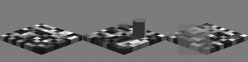
A new approach to measuring LTFs was suggested by the recent paper of Allred et al. (Reference Allred, Radonjic, Gilchrist and Brainard2012) who measured what they termed context transfer functions with a two-dimensional checkerboard in the fronto-parallel plane. They measured how the perceived lightness of the central check changed as a function of variations in the luminance range of the near and far adjacent checks. A novel feature of the experimental design of Allred et al. (Reference Allred, Radonjic, Gilchrist and Brainard2012) was to randomize the arrangements of the surrounding checks. Then they measured the average response to a given check, averaged over many different surrounds that were drawn from the same ensemble. Allred et al. did not arrange the surroundings to create a heightened or diminished perception of lightness but rather measured lightness on the average. We adopted a similar strategy to measure the LTF. We used somewhat more naturalistic stimuli in which the geometry of the checkerboard pattern was arranged so as to create a linear perspective view of an apparently three-dimensional checkerboard that was slanted in depth (Fig. 1). With checkerboard stimuli like that in Fig. 1, we tested the effect on the LTF of different illumination situations, specifically plain view, a cast shadow, and an intervening transparent medium.
Checkerboard stimuli and experimental variation of scene context. Left: checkerboard composed of ten by ten checks with ten different reflectance values. Middle: checkerboard with shadow-casting cylinder. Right: checkerboard with transparent medium superimposed.

The LTF is just one example of a more general psychophysical problem (Fechner, Reference Fechner1860) of how a psychological experience [in this case, apparent lightness denoted Ψ(x)] is linked by intervening neural processing to physical variables (in this case, we initially used the physical variable luminance denoted x). The problems we encountered in trying to determine the transformation from x to Ψ(x) are likely to arise for measurements of all kinds of different sensation magnitudes. Based on our data on the computation of perceived lightness from luminance, we will discuss two methodological issues: (a) how does one find what is the appropriate physical variable (what is the right x?) to look at and (b) how can we use our measurements to probe the internal transformation that leads to appearance.
Materials and methods
Observers
Four observers with an age range of 24–34 years participated in the experiment. Two of them were males. All observers had normal or corrected-to-normal visual ability. Observers were reimbursed for their participation.
Stimuli and apparatus
Stimuli were presented on a linearized 21″ Siemens SMM21106LS monitor (400 × 300 mm, 1024 × 766 pixel, 130 Hz) controlled by a DataPixx (VPixx Technologies Inc. Saint-Bruno, QC, Canada) and custom presentation software developed in our lab and published at https://github.com/TUBvision/TUBvision/hrl. The maximum luminance the setup could produce was 549 cd/m2.
Stimuli were 2D perspective projections of a checkerboard rendered with Povray, which is a general-purpose ray tracing-based rendering software (Persistence of Vision Pty. Ltd., 2004, Williamstown, Victoria 3016 Australia). With rendered images, the user has no direct control over the pixel intensities in the rendered images (gray values), but only specifies the desired reflectance values in the description file. One of ten possible surface reflectance values was assigned randomly to each of the checks, except for the surface colors at the target locations that were specified by the design.
In the shadow condition, a cylinder was positioned on the horizontal diagonal and toward the right half of the checkerboard (see Fig. 1). The cylinder’s shadow covered about 17 of the 100 checks. In the transparent condition, a transparent medium covered an area of about 48 of the 100 checks. Povray description files were generated automatically with Python, and Povray was also executed from within Python. The resulting images were subsequently converted to a gray scale matrix and normalized to contain values between 0 and 1.
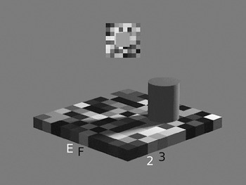
All stimuli were created prior to the experiments and loaded later for presentation. Images subtended 17.3 × 13° visual angle. The checkerboard was rotated by 45° so that one of its major diagonals was parallel to the x-axis and the other extended in an imaginary z-axis (depth). The horizontal main axis subtended 17.2° and the vertical main axis 6.8°. Individual checks had an edge length of about 0.9° visual angle. The comparison field (Fig. 2) was presented on a local checkerboard background that was randomly generated from trial to trial but constant during the adjustment within a trial. The intensities of the single checks in the comparison checkerboard were drawn from 20 different equally spaced luminance values between 11 and 473 cd/m2. Observers were seated 80 cm away from the screen, and their head position was fixed with a chin-rest. Responses were recorded with a ResponsePixx button-box (VPixx Technologies Inc. Saint-Bruno, QC, Canada). The experimental setup was located in an experimental cabin that was dark except for the light emitted by the monitor.
Stimulus display in a single trial. The checks of interest E3, F2, and F3 are indicated by letters and numbers, and the current check of interest E2 is indicated in white. The comparison field is shown above the test stimulus on its own local checkerboard surround.

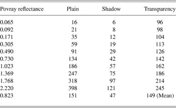
The stimulus luminances given in Table 1 were measured by means of a Konica Minolta LS-100 spot luminance photometer (Osaka, Japan) which in combination with a 122 close-up lens allows measurements of spot sizes down to 3.2 mm. The photometer was mounted on a tripod (Manfrotto, Cassola, Italy) and was connected via a serial port (RS-232C) to the presentation software. The measurements were performed in a semiautomatic way, because the photometer was focused by hand on the three checks of interest (F2, F3, E3), and then the ten different reflectance values were presented under each of the viewing conditions while the photometer automatically read the emitted luminance values which were registered by the computer. Each measurement was repeated 12 times, and the highest standard error of the mean of 2.8 cd/m2 was measured for the highest luminance in the plain condition (398 cd/m2). In plain view, the luminance range we studied corresponded with the range of luminances measured in natural scenes (Laughlin, Reference Laughlin1981).
Luminance values in cd/m2 corresponding to the ten different check reflectance values when the checkerboard is rendered in different contexts

Design
The variable that was manipulated was the type of viewing context, that is, plain view, shadow, or transparency. All observers were exposed to all three viewing contexts. Apparent lightness was judged for ten different check-reflectance values which differed in luminance depending on the viewing context in which they were presented as specified in Table 1. The ten reflectance values for the checks were chosen such that the resulting luminance values were approximately equidistant in lightness when viewed as simple squares next to each other on the mean background intensity (200.2 cd/m2) of the linearized experimental monitor. The mean luminance of the checks in each context is given in the last row of Table 1. Six of the check luminances were below the mean; four were above the mean.
Procedure
Observers made 12 adjustments for each of the ten reflectance values in each of the three viewing conditions. The checkerboard rows were denoted a–j and the columns were denoted 1–10. The three checks of interest were checks E3, F2, and F3; their rows and columns were labeled with black letters and numbers during the experiment as indicated in Fig. 2. These checks were chosen because they were located well within the region of either the shadow or the part of the checkerboard seen through the transparent filter. For each checkerboard stimulus, the apparent lightness of each of the three checks of interest was evaluated one after another. The labels of the relevant check were colored white so that the observer knew which check was currently to be judged. The labels were shown outside the checkerboard, and hence, it is unlikely that they exerted any effect on perceived check lightness. Observers adjusted the perceived lightness of a comparison field, presented above the checkerboard on its own local checkerboard background, by pressing one of the four buttons. Two of the buttons decreased or increased the comparison intensity by 5%, and the other two buttons by 0.5%. Observers indicated a satisfactory match and initiated the next trial by pressing a fifth button at the center of the response box. Observers performed all trials within one session. Their progress was indicated at the bottom right of the display.
Results
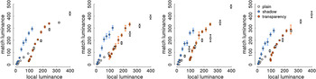
We will present the matching data graphically. They will be replotted several times with different variables on the x- and y-axes. Figs. 3–6 are organized analogously with the following conventions. Data from different observers are plotted in different panels and data from different scene contexts are coded in different colors. Fig. 3 shows the LTFs when test and comparison field intensity are plotted in units of local luminance. For the checkerboard in plain view, the transfer function followed the identity line (slope = 1.08, intercept = −2.5, R 2 = 0.99; the parameters were calculated for each observer and then averaged to show the mean results). For the apparent lightness of the checks viewed in the shadow, the mapping function had a steeper slope (slope = 2.6, intercept = −2.4, R 2 = 0.97). The reduced range of check luminances within the shadow (x-axis) was mapped to almost the same range of comparison luminances that was observed for the checkerboard in plain view. The same was true for the checkerboard viewed through the transparent medium. Here the range of possible check luminances was reduced and shifted upwards along the x- axis resulting mainly in an intercept change of the transfer function relative to that in plain view (slope = 1.97, intercept = −129.8, R 2 = 0.96). Thus, when plotted in luminance–luminance space, the transfer functions in different contexts differed in slope and intercept (or, in other words by a multiplicative and a subtractive factor). Note that the data replicate observations of others. For instance, for checks in the shadow condition, the same check luminance (e.g., 50 cd/m2) was perceived as much lighter than in plain view, replicating previous observations with a similar display (Adelson, Reference Adelson and Gazzaniga2000).
Empirically derived transfer functions of individual observers. Matching luminance is plotted as a function of local target luminance. Data from different conditions are color-coded, and single data points are the average of 12 match settings for each of the ten possible target luminances.

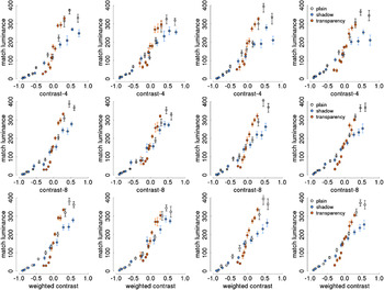
Empirically derived transfer functions of individual observers plotting matching luminance as a function of the luminance contrast of the target check relative to its respective surrounding checks. Contrast was calculated as (L check − mean(L surround))/(L check + mean(L surround)). Contrasts were divided into ten bins with 12 observations each. Upper row—surround luminance is calculated as the average of the four adjacent check luminances. Middle row—surround luminance is calculated as the average of the eight adjacent check luminances. Lower row—surround luminance is calculated as a weighted average of the surround luminances with the near check luminances (adjacent edge) being weighted twice as much as the far check luminances (adjacent corner). Error bars indicate standard errors of the mean.

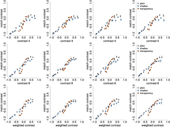
Empirically derived transfer functions of individual observers plotting matched test contrast as a function of the luminance contrast of the target check relative to its respective surrounding checks. Panels are organized as in Fig. 4.

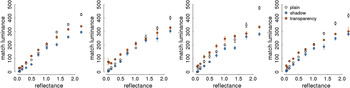
Reflectance matching in different contexts. For each observer, the graph plots the matching luminance as a function of the surface reflectance values as they were specified in the description file of the rendering program.

If the same luminance looks different in lightness because of context, then one might expect that the observed variance in matching luminance would be reduced when, instead of luminance, some other variable is plotted on the x-axis that explains part of the observed variance. One often proposed and easy-to-compute candidate variable would be luminance contrast instead of luminance itself (Wallach, Reference Wallach1948). Therefore, in Fig. 4, the matching data are plotted as a function of contrast instead of luminance. We calculated a modified Rayleigh-contrast in which the luminance difference between the check of interest and its surrounding checks was expressed relative to their sum: C = (L check − mean(L surround))/(L check + mean(L surround)). [We also analyzed the data in terms of Weber contrast, i.e., (L check − mean(L surround))/(mean(L surround)) and found a slightly worse fit across contexts. We also computed the average Rayleigh contrast <C>, averaging across the Rayleigh contrasts of the four adjacent checks or eight nearest checks and obtained results that were the same as for the modified Rayleigh contrast results presented here in terms of L surround]. Surround luminance (L surround) was calculated in three different ways. For the contrasts plotted in the upper row of Fig. 4, the surround luminance was determined by averaging the luminance values of the four checks that shared an edge with the test check (contrast-4). Contrasts in the middle row of Fig. 4 were calculated with surround luminances that were an average of the luminance of all eight adjacent checks (contrast-8), not only those four that shared an edge (near) but also those four that shared a corner (far) with the test check. The lowest row of plots in Fig. 4 depicts contrasts that were a weighted average of the eight adjacent check luminances (weighted-contrast), with near check luminances being given double the weight of far check luminances (1/6 vs. 1/12 to each individual check). The resulting contrast values were combined into bins containing 12 values each (to be comparable with the luminance data for which data were averaged across 12 repeats). Naturally, that type of binning resulted in different bin positions along the contrast dimension between conditions. However, binning according to the same number of elements, as opposed to binning in equidistant units in contrast space, has the benefit that variability differences between the bins are interpretable.
Fig. 5 follows the same logic as Fig. 4 but here both the stimulus intensity on the x- axis and the comparison field intensity on the y-axis are expressed in terms of local contrast. At the time the experiment was performed, we did not anticipate that the contrast might be of interest, and hence we did not save the intensities of individual fields in the randomized comparison surround. Therefore, the contrast measure for the surround of the comparison stimulus is rather crude. The surround luminance value was simply the mean intensity of all the fields in the comparison checkerboard (242 cd/m2). Due to that constant surround luminance, the upper limit of possible comparison contrasts was set as 0.39 (L max − L surround/L max + L surround). The maximum luminance (L max) of our display was 549 cd/m2 (see Materials and methods). Visual inspection of Fig. 5 suggests that converting the ordinate into contrast values made the data even more compatible with a single underlying transfer function.
Comparing Fig. 3 with Figs. 4 and 5, one can see that the qualitative differences (slope and intercept) between LTFs in different contexts in Fig. 3 have disappeared. For the contrast-8 and the weighted-contrast measure, it is not so obvious from the graphs which one is more consistent with a single transfer function. One needs to compare quantitatively to what extent the data from different contexts are compatible with a single transfer function when different choices of x- and y-axes are used. To perform this comparison, we computed two types of indices. Table 2 summarizes results with one index, which we call the global R 2. The global R 2 is the proportion of variance explained by a linear model that was fitted to the data from all contexts (“pretending” the data originated from a common model, although evidently that is not true for the data in Fig. 3). The so-computed global R 2 can then be compared with the R 2s that result when fits are performed for each context separately (see Table 2), and the smaller the difference between the global and the separate R 2s, or the higher the global R 2, the more the data are compatible with a single underlying function.
R2 calculated separately for each context condition and for all data across context conditions (global R2)

The results in Table 2 indicate that the best fit to a single global transfer function was achieved when the data were plotted on the axes (contrast-8, contrast) or (contrast-w, contrast) because for those choices of axes, the global R 2 was highest and close to the R 2 for the best fit to the individual contexts. The (luminance, luminance) graph had the worst fit to the global single function because its R 2 was substantially lower than the linear fits to the data for the individual contexts.
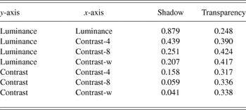
A second index for quantitative comparison of the transfer functions was called the prediction benefit, calculated as follows: (1) A linear model was fit to the plain-view data because these can be regarded as a type of ideal performance. (2) Then the regression coefficients for the plain-view data were used to predict the matching values for the shadow and the transparency data. (3) The residual variance after this fitting was then calculated based on the differences between the actually observed data points in the respective context and the predicted data points from the plain-view condition. (4) The residual variance was divided by the total variance of matching values in that context to arrive at the prediction benefit. We normalized the residual variance by the total variance in the respective context because the total variance can be interpreted as the mean squared differences from the condition mean or from a line with zero slope and intercept equal to the mean. The prediction benefit captures the reduction in prediction error for values predicted by plain-view parameters relative to a prediction based on the mean in the respective condition. Smaller values of prediction benefit mean that the data in that context (shadow, transparency) were better fit by the plain-view parameters than by the condition mean. Results are tabulated in Table 3. With prediction benefit one observes that the shadow data were very well fit by the same straight line that fit the plain-view data for (contrast, contrast-8) and (contrast, contrast-w). However, the transparency data were consistently not well fit by the line derived from the plain-view data.
Prediction benefit calculated as the proportion of residual variance relative to the total variance of the data in the respective conditions. The residual variance is based on residuals that were calculated as the difference between the actual data and data predicted from a linear fit to the plain-view data (see text for details)

The observers exhibited a high degree of lightness constancy in their performance. Fig. 6 depicts matching luminance as a function of the surface reflectance values as they were specified in the description file of the rendering program. The data in the plain-view condition can be regarded as a reference. Observers are not perfectly lightness constant as indicated by the fact that the data from the shadow and the transparency conditions are below those in the plain-view for the three highest reflectance values. However, up to that point, the data are matched pretty constantly and consistently higher than what would be expected based on the respective check luminances in the different viewing conditions (for comparison, see Table 1).
Discussion
We will now, on the basis of the observed results, address the two problems that we raised in the Introduction associated with measuring and interpreting the mapping between a proximal stimulus (luminance) and its corresponding perceptual attribute (lightness).
Choosing the right physical dimension might be easy when simple stimuli, such as isolated spots of light, are concerned. However, even then it has been noted that ‘... more than one set of rules may be usefully applied to the same subject matter; for example, both dynes/cm2 and decibels are valid measures of sound pressure. Neither is the “correct” scale: we choose between them according to their usefulness or the facility of the measuring operations required’ (p. 12, Treisman, Reference Treisman1964). Clearly, when the stimulus becomes more complex, like surfaces in different illuminations, it will become an empirical question what is or are the right input dimension(s) to look at. Consequently, the interpretation of the data will be quite different.
In the present paper, we measured the luminance to lightness mapping in a stimulus that, as in natural scenes, contained geometric cues that were associated with an impression of depth and with different illumination situations, namely a cast shadow and a transparent medium. When we parameterized the luminance to lightness mapping in the different viewing situations in a luminance–luminance space (Fig. 3), the data seemed to indicate qualitative differences in the mapping functions, since they differed in both slope and intercept. This was consistent with earlier reports that modeled similar data with a multiplicative gain and subtractive offset model (e.g., Allred et al., Reference Allred, Radonjic, Gilchrist and Brainard2012). The local luminance that excites a photoreceptor is the proximal stimulus by which the visual sensors make contact with the external world. However, it has often been suggested that the visual system translates absolute luminance information into a relative luminance or luminance contrast signal (Wallach, Reference Wallach1948; Whittle & Challands, Reference Whittle and Challands1969; Shapley & Enroth-Cugell, Reference Shapley, Enroth-Cugell, Osborne and Chader1984). We thus replotted the transfer function in different coordinate systems with different versions of luminance contrast on the x- and y-axes. We found that the qualitative differences between mapping functions in different contexts were substantially diminished when the data were plotted in terms of contrast.
On contrast–contrast coordinates, the data were compatible with a single linear generative model as we observed determination coefficients (R 2) of 0.91. We think it is interesting that relatively complex scene changes, and their accompanying changes in the perceived lightness of image regions, could be captured to a large extent by as simple a measure as luminance contrast. However, it is important to note that the contrast measure employed here was not purely a local image-based contrast measure. There was a substantial benefit for explaining the perceived lightness of the target check when, in addition to the four directly adjacent checks, also the four more remote checks which only shared a corner with the target check were considered (the contrast-8 or contrast-w calculations). Our findings on the influence of the corner checks are consistent with earlier work that found an effect on perceived lightness of somewhat more remote context (Reid & Shapley, Reference Reid and Shapley1988; Rudd & Zemach, Reference Rudd and Zemach2004).
The data on lightness matches for the transparent condition suggest that more complicated neural computations were employed by the observers when they judged lightness through transparency. The deviation of the transparency data from the plain-view and shadow data is quite evident in Figs. 4 and 5. Furthermore, the prediction benefit computations in Table 3 imply that lightness perception though transparency is quantitatively different from shadow and plain-view. This suggestion is consistent with the conclusions of Singh (Reference Singh2004) about lightness perception through transparent media. However, the detailed lightness settings between the two studies are difficult to compare because the spatial contexts of Singh (Reference Singh2004) and ours were very different. We only used a single transparent condition in which the transparent medium had a high reflectance so that the mean luminance of the checks in the transparent condition was increased compared with the plain-view condition. In future, it would be desirable to undertake a more complete study of lightness perception through transparency, with many different transparent media and with the use of the statistical averaging approach we have used here.
The high correlation we found between the weighted contrast measure and perceived lightness appears to conflict with many recent studies of lightness perception (reviewed in Gilchrist, Reference Gilchrist2006; Kingdom, Reference Kingdom2011). It is possible that the results reported here were obtained because we used an experimental procedure that was different from the approach used in many previous studies. For example, Allred and Brainard (Reference Allred and Brainard2009) used a target that was not embedded within a surface of similar elements and found that perceived lightness was well predicted by local contrast under some conditions and not others. Our stimuli were randomized checkerboards and the observers were judging the lightness of target checks embedded within the same surface as the spatial context around the target checks. The use of the random checkerboards (following the experimental design of Allred et al., Reference Allred, Radonjic, Gilchrist and Brainard2012) allowed us to measure lightness judgments under a more generic situation than that used in other studies of lightness perception.
It is also worth noting that Blakeslee and McCourt and their colleagues (for instance, Blakeslee et al., Reference Blakeslee, Reetz and McCourt2009) found that the perceived lightness of many visual stimuli could be predicted by their ODOG (Oriented Difference of Gaussians) model, which is a multiscale spatial-filter model that computes spatial contrast at many spatial scales. However, the finding that the weighted contrast measure was highly correlated with perceived lightness does not imply that contrast is the crucial cue for assigning lightness to retinal image regions. Rather, contrast might be highly correlated with whatever factor(s) will turn out to be crucial for assigning lightness to retinal image regions.
The dependence of lightness perception on adjacent and nearby checks could be interpreted as a support for the idea that the neural computations of lightness are strongly influenced by local computations in the primary visual cortex, V1. Several previous studies have shown that responses to visual patterns in V1 resemble lightness perception qualitatively and quantitatively (Kinoshita & Komatsu, Reference Kinoshita and Komatsu2001; MacEvoy & Paradiso, Reference MacEvoy and Paradiso2001; Haynes et al., Reference Haynes, Lotto and Rees2004; Paradiso et al., Reference Paradiso, Blau, Huang, MacEvoy, Rossi and Shalev2006). Such an interpretation of our data does not preclude that there are significant influences of neural computations beyond V1. There are many phenomena of lightness perception that probably require an explanation in terms of longer distance interactions and higher-order interactions (reviewed in Gilchrist, Reference Gilchrist2006; Kingdom, Reference Kingdom2011). However, in the contexts we used in our experiments, and with the checkerboard displays used (Fig. 1), the nearest-neighbor and next-nearest-neighbor interactions were sufficient to account for most of the lightness variation (Tables 2 and 3).
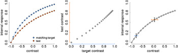
How to estimate the internal psychological variable that represents lightness is the second major problem that needs to be considered. Often the appearance of a target region is probed by having observers adjust the appearance of a comparison region, and the average adjustments of the comparison intensity are interpreted to be indicative of the appearance of the target. This is what we did in measuring the LTFs (cf. Adelson, Reference Adelson and Gazzaniga2000; Allred et al., Reference Allred, Radonjic, Gilchrist and Brainard2012). The problem with that logic is that the functions relating stimulus intensity (x) to internal response (Ψ (x)), at both target and comparison regions, are not being measured directly. Instead, one measures the stimulus intensities of the comparison region that match different stimulus intensities of the target region. The resulting measurements only show how the x-axes of the actually interesting Ψ functions relate to each other when their respective function values are being matched. The idea is illustrated graphically in Fig. 7. It is assumed that the internal magnitude of perceived lightness is a saturating function of luminance. It is additionally assumed that the functions relating luminance and perceived lightness at the target and at the comparison regions have a similar shape, although it is possible that they might saturate at different levels (Fig. 7, left panel). From the adjustment data, which is the only thing we can measure in a standard adjustment procedure, the shape of the curves would not be evident (Fig. 7, central panel) because all that is available to the experimenter are the respective contrast values of the two curves shown in the left panel of Fig. 7.
Illustration of the problem of measuring internal responses. Left: hypothetical curves relating local luminance contrast of an image region (x-axis) to an internal response such as the one that corresponds to the perceived lightness of the image region. Data were generated with three parameter Naka–Rushton functions with n = 1, R_max = 1, and sigma_match = 0.5 and sigma_test = 0.8. Middle: the points from the two curves in left panel are scatter-plotted against each other and expressed in their respective contrast coordinates. Right: illustration of how equal variances on the internal response (y axis, black error bars) relate to variances that increase with increasing stimulus intensities (x-axis) for a function that is compressive toward the upper asymptote. The blue and red error bars indicate the variance range on the x-axis that relates to constant variances on the y-axis.

The problem of estimating internal magnitude from adjustment data has been noticed before. For example DeValois et al. (Reference DeValois, Webster, DeValois and Lingelbach1986), studying the temporal properties of brightness induction, wrote that “In the static situation both the inspection and matching patterns may well be subject to adaptation. This could perhaps reduce the salience of both of the patterns while not altering the match between them.” A similar problem is encountered in scaling experiments where instead of having direct access to Ψ(x), observers provide response magnitudes, which are themselves a function of Ψ(x), and thus, only indirectly related to x (Treisman, Reference Treisman1964; Shepard, Reference Shepard1981). We think that by looking also at the variability in addition to the mean matching responses one might get closer to the underlying response curves. The idea is illustrated in the right panel of Fig. 6 and the underlying linking assumptions are summarized in Fig. 8.
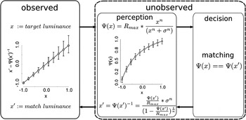
Linking assumptions underlying matching procedures. The left part of the diagram depicts the data that can be measured (observed) in a matching procedure: the match luminance of a test region (x′) as a function of the luminance of a target region (x). The right part of the diagram depicts the putative hidden mechanisms (unobserved) and is divided into a perception and a decision part. In the perception part, it is assumed that there exists a mapping function that relates some percept (Ψ(x)) to the physical variable (x, upper equation following the upper rightward arrow). Of course, in the matching experiment scenario, there are two such mapping functions, one for the target and one for the test stimulus (see also Fig. 6). The shape of these mapping functions is not known but they are often modeled with the so-called Naka–Rushton function which is employed to characterize the relation between Ψ(x) and x also here. The decision mechanisms involve a comparison between Ψ(x) and Ψ(x′). Once a matching has been accomplished, the mapping function needs to be inverted because the percept (Ψ(x′)) needs to be translated into the corresponding physical stimulus x′ which the experimenter can measure (lower leftward arrow).

One may be able to estimate the shape of the true luminance-to-lightness mapping functions by considering the variance at different levels of the physical intensity variable. This requires one to make assumptions about the underlying response mechanism (Pelli, Reference Pelli1985). The internal variable [apparent lightness, Ψ(x)] should increase monotonically with the physical variable (luminance or contrast). The variability in the internal variable results from an “additive” noise source, that is, the variability is independent of the intensity level of the internal variable (in contrast to a “multiplicative” noise term, where the internal variability would be proportional to the overall intensity). If the internal variability was independent of the level of Ψ(x), then differences in variability in the physical variable x can be attributed to a nonlinear underlying transfer functions because the equal variability in Ψ(x) would map to unequal variability in x due to different local slopes. This is illustrated in Fig. 7 where the same amount of variation at high intensities would lead to more variability in the x-axis (red error bar) than at low intensities (blue error bar). Fig. 8 depicts the linking assumptions that are necessary to relate observer behavior to internal response mechanisms. The left box shows the kind of data that are measured in a matching task. The right box is a black box model of the human observer in a matching task. The matching process starts with the mapping from physical stimulus intensity to internal response (apparent intensity). An often-used nonlinear response function for light intensity variations is the Naka–Rushton function (e.g. Hillis & Brainard, Reference Hillis and Brainard2007). The data points and the response curve (Ψ(x)) in Fig. 8 were generated with the equation that is written in the figure. In the matching experiment scenario, there are two such internal response functions, one for the target and one for the test stimulus (see also Fig. 7). The matching is performed between the respective outputs of the response functions at the target (Ψ(x)) and the test position (Ψ(x′)). Once a match has been reached, the percept (Ψ(x′)) needs to be translated back into the corresponding physical stimulus x′, which the experimenter can measure (lower leftward arrow). That is accomplished by inverting the response function (lower equation in Fig. 8). The data points and error bars in the plot on the left (observable) part of Fig. 8 have been obtained by assuming identical internal response curves at test and match positions and by inverting the error limits associated with each point of the response curve (right, unobservable part of Fig. 8). Thus, assuming a Naka–Rushton type internal response function at both test and match positions would produce a linear relationship between test and match luminance and variability estimates that increase with increasing test luminance. In the present data, a relationship between test intensity and variability of the match could be suspected for the plots in luminance–luminance and luminance-contrast coordinates (Figs. 3 and 4), but not for the contrast–contrast data (Fig. 5). However, the present data do not allow for a quantitative test of the supposed relationship between variability and intensity because not enough data were collected per data point, and, unlike luminance, the contrast bins were calculated only posthoc, and hence contain a mixture of different contrast values.
The present results and the reasoning about matching procedures suggest that the mean settings are important to determine the appropriate input dimension, that is the horizontal axis of an internal response function because they provide similarity judgments. For judging the representation of the internal variable, that is the vertical axis of that same function, one has to consider also the variability of the settings because with matching there is no intrinsic metric on the output scale.
There is another approach to measure appearance, namely, scaling where observers assign numerical values to apparent intensities (e.g. Gescheider, Reference Gescheider1988). But scaling has no guaranteed metric either. In scaling procedures, observers assign numbers to stimulus intensities (category scaling or magnitude estimation) or they produce multiples or fractions of a certain stimulus intensity (ratio production). However, the observed response is comprised of two component functions: one, which has been called the stimulus function (Treisman, Reference Treisman1964), relates the physical stimulus intensity (I) to an internally evoked sensation (Ψ(I)). This function C = f(I) is the function that we are genuinely interested in. The second component is the response function, which relates the response that we can measure to the internally evoked sensation, R = g(C) = g(f(I)). So, again, there is no direct access to the internal response function. Scaling has been validated practically by its consistency. However, one can consistently measure a variable that has no validity, and the consistency might have been artificially high, because observers might remember the numerical labels that they have used previously in response to a certain stimulus. In future, it might be worthwhile to collect data in scaling and matching experiments in a way that allows the analysis of variability in addition to mean data. For variability data to be interpretable, the following precautions should be taken. The starting values of a matching stimulus should be randomized. In addition, the entire sequence of match settings should be saved and analyzed, instead of the final matching value only. This is because even if the initial match intensity is randomized, observers might use an internal or external reference to which they match the comparison first and then start from this ad-hoc reference to match the target. Such a strategy could then at least be identified. Second, if observers are to choose from a given number of comparison stimuli and these are sorted and/or labeled, then it is easy for observers to produce highly reliable matches over repeats of the same test intensity because they might have memorized their previous choice. A solution to the problem may be to randomize the arrangement of comparison intensities from trial to trial and to abstain from labeling.
Acknowledgment
This work has been supported by an Emmy-Noether research grant of the German Research Foundation to Marianne Maertens (DFG MA5127/1-1) and an NIH grant to Robert Shapley (R01 EY 1472). We are grateful to Katharina Zeiner who collected the data and to Katharina Zeiner and Torsten Betz for comments on an earlier version of the manuscript. We would also like to thank James Gordon and Felix Wichmann for helpful suggestions.