1. Introduction
The flow past arrays of long solid obstacles is important for many applications in fluid mechanics. Common examples include bridge piers with multiple piles and other types of offshore structures supported on arrays of piles (Ball, Stansby & Allison Reference Ball, Stansby and Allison1996), arrays of turbines in a wind farm and finite patches of vegetation (Nepf Reference Nepf2012; Zong & Nepf Reference Zong and Nepf2012). In most of these practical applications, the solid obstacles can be modelled as cylinders of a simple shape (e.g. circular or square), and the number of solid cylinders of diameter
 $d$
that form the array (
 $N$
) is relatively large (
 $N>20$
), such that wake-to-cylinder interactions are significant within the array and well-defined separated shear layers (SSLs) are generated on the lateral sides of the array. For such cases, the region containing the cylinders is formally equivalent to a porous medium with close-to-uniform porosity. In relatively many cases, the array has a close-to-circular shape (figure 1). Classical examples are multiple-pile bridge piers and patches of vegetation in the initial stage of growth (Vandenbruwaene et al.
Reference Vandenbruwaene, Temmerman, Bouma, Klaassen, de Vries, Callaghan, van Steeg, Dekker, van Duren, Martini, Balke, Biermans, Schoelynck and Meire2011; Chen et al.
Reference Chen, Ortiz, Zong and Nepf2012). Of particular interest for practical applications are cases where the Reynolds number defined using the diameter of the array,
 $D$
, and the mean incoming velocity,
 $U$
, is larger than approximately 2000, such that the wake generated by the array is turbulent. An understanding of the physics of the flow past circular porous patches is fundamental to the general understanding of flow through porous patches of more complex shape. Moreover, the limiting case of flow past a solid cylinder has been widely studied in the literature (Williamson Reference Williamson1996; Zdravkovich Reference Zdravkovich1997).
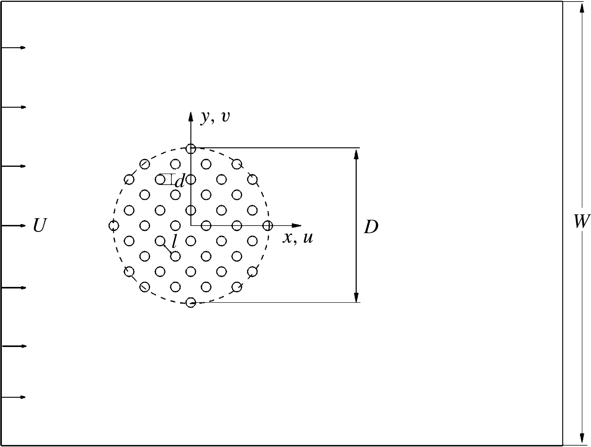
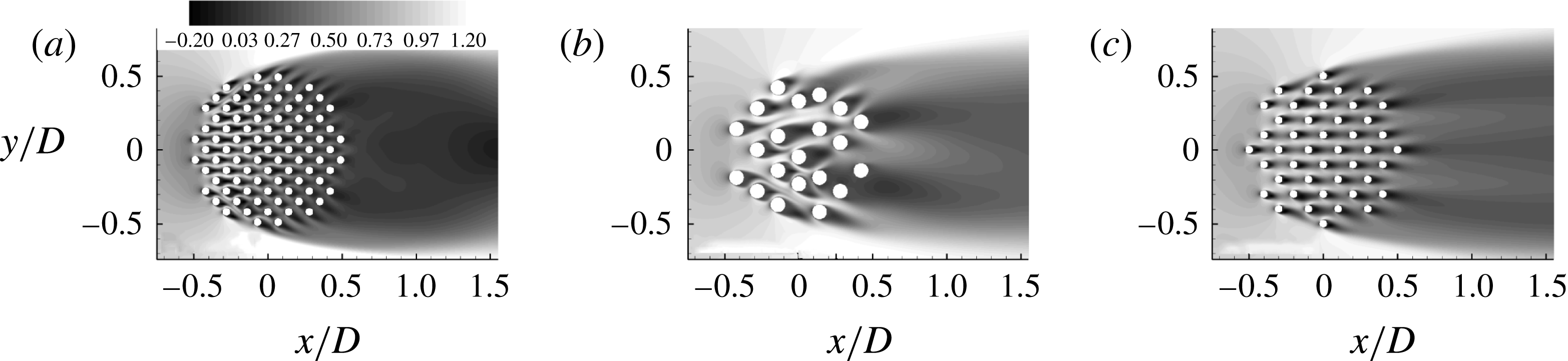
Sketch of the computational domain containing a porous cylinder of diameter
 $D$
. The diameter of the solid cylinders is
 $d$
and the average distance between the solid cylinders is
 $l$
. The domain width is
 $W$
and the uniform incoming velocity is
 $U$
. The velocities in the streamwise and spanwise directions are denoted
 $u$
and
 $v$
, respectively. The sketch is not to scale as
 $W=14D$
in the simulations.

In a fairly good approximation, for sufficiently large
 $N$
and for cases where the position of the rigid cylinders in the array is not exactly regular, circular arrays also have the advantage of eliminating the angle of attack of the incoming flow relative to the array as a main variable to be considered in the study of the flow physics. Compared with the case of a solid cylinder, flow past porous cylinders is characterized by a bleeding flow through the array. The bleeding flow penetrates in between the SSLs of the porous cylinder. The stronger the bleeding flow, the longer the distance at which the ends of the SSLs can interact. For a sufficiently high volume fraction of solids (SVF), this interaction results in the alternate shedding of wake billow vortices (von Karman vortex street) via the same mechanisms as observed for solid cylinders. The distance between the back of the porous cylinder and the streamwise location where the wake billow vortices form is called the steady wake region (Zong & Nepf Reference Zong and Nepf2012). For sufficiently low SVF, no vortex street is observed for the porous cylinder. In this study, the SVF is defined as the ratio between the total volume of the cylinders in the array and the volume of the porous cylinder of diameter
 $D$
.
The present study was to a large degree motivated by the need to understand the effect of patches of emerged aquatic vegetation present in the main channel of streams or over their floodplains. Patches of aquatic vegetation are ecologically important as they retain nutrients and trap heavy metals and polluted sediments transported in the water column (Sand-Jensen & Pedersen Reference Sand-Jensen and Pedersen2008; Neary et al. Reference Neary, Constantinescu, Benett and Diplas2012). In many river restoration and bank stabilization projects, vegetation is planted in dense uniform patches to control the patterns of scour and deposition (Bennett, Pirim & Barkdoll Reference Bennett, Pirim and Barkdoll2002; Bennett et al. Reference Bennett, Wu, Alonso and Wang2008; Nepf Reference Nepf2012). This is one of the reasons why we consider patches of uniform porosity in this study. Natural streams generally contain many patches of (emerged) vegetation. However, if the ratio of the average distance between two patches to the ‘mean diameter’ of the patch is sufficiently high, the patch-to-patch interaction is negligible and the study of flow past isolated patches, as done in the present study, is relevant. In many previous investigations of flow in vegetated channels, rigid circular cylinders of constant diameter have been substituted for individual plant stems (Chen et al. Reference Chen, Ortiz, Zong and Nepf2012; Zong & Nepf Reference Zong and Nepf2012). This is also the approach adopted in the present numerical study.
Most previous experimental studies of flow past groups of cylinders considered only the interaction between a small number of solid rigid cylinders (
 $N<10$
) placed either side by side or one behind the other (see Lam, Li & So (Reference Lam, Li and So2003) and Takemura & Tanaka (Reference Takemura and Tanaka2007) for a review). Such configurations are not exactly representative of the complex interactions observed within a porous patch that contains a large number of cylinders. The flow past a patch containing seven circular emerged cylinders of constant diameter
 $d$
was investigated experimentally by Takemura & Tanaka (Reference Takemura and Tanaka2007). The total drag force on the porous cylinder and the Strouhal numbers associated with the vortex shedding past the solid cylinders and in the wake of the porous cylinder were measured in their water flume experiments. The study investigated the changes in the flow and drag forces with the angles of attack and ratio
 $l/d$
(
 $=0.25$
to 5), where
 $l$
is the mean distance between the surfaces of two neighbouring cylinders (figure 1). The solid cylinder Reynolds number,
 $\mathit{Re}_{d}=Ud/{\it\nu}$
(
 $U$
is the mean incoming flow velocity,
 ${\it\nu}$
is the viscosity), was varied between 400 and 4000. Other studies considered patches with a much larger number of cylinders (e.g. Ball & Hall (Reference Ball and Hall1980) studied a square patch containing 81 cylinders), but the investigation was limited to estimating the total drag force acting on the porous cylinder. Several experimental studies concentrated on the wake structure downstream of porous obstacles (circular cylinders and flat plates) and in particular on determining the critical value of the SVF below which the von Karman vortex street is suppressed (Castro Reference Castro1971; Chen & Jirka Reference Chen and Jirka1995; Huang & Keffer Reference Huang and Keffer1996).
Such a study focusing on circular porous cylinders containing a large number of solid emerged finite-length cylinders placed in a water flume was recently reported by Zong & Nepf (Reference Zong and Nepf2012). The study analysed the changes in the near-wake structure, dominant wake frequencies, lengths of the steady wake and total wake regions with the SVF (
 $0.03\leqslant \text{SVF}\leqslant 0.36$
),
 $d/D$
(
 $0.014\leqslant d/D\leqslant 0.05$
) and the porous cylinder Reynolds number (
 $10^{4}\leqslant \mathit{Re}_{D}=UD/{\it\nu}\leqslant 4\times 10^{4}$
,
 $\mathit{Re}_{d}\approx 500$
). Theoretical models were proposed to determine the length of the steady wake region and the mean streamwise velocity along the centreline within this region. Additional similar data are provided by the experimental study of Chen et al. (Reference Chen, Ortiz, Zong and Nepf2012) for
 $0.03<\text{SVF}<0.51$
and
 $0.015<d/D<0.128$
.
Nicolle & Eames (Reference Nicolle and Eames2011) used highly resolved two-dimensional (2D) direct numerical simulation (DNS) to study the flow structure within and downstream of a circular porous cylinder containing between seven (
 $\text{SVF}=0.016$
) and 133 (
 $\text{SVF}=0.3$
) circular cylinders and to estimate the effect of the SVF on the drag forces on the individual cylinders and the structure of the flow within and past the porous cylinder. Such simulations correspond to the case of long cylinders, as periodic boundary conditions were used in the vertical direction. Flow structure predicted by such simulations is expected to be similar to that observed away from the channel bed in experiments conducted in open channels of finite depth, provided that bed roughness plays a negligible effect on the development of the porous cylinder wake (flow shallowness effects are negligible, Chen & Jirka Reference Chen and Jirka1995). The numerical study of Nicolle & Eames (Reference Nicolle and Eames2011) was conducted with solid cylinders of constant diameter
 $d=0.048D$
at a relatively low Reynolds number (
 $\mathit{Re}_{d}=100$
,
 $\mathit{Re}_{D}=2100$
). For such cases, 3D effects (e.g. via vortex stretching) are expected to be relatively small, at least inside and close to the porous cylinder. Their 2D DNS showed that for
 $\text{SVF}<0.05$
the cylinders have close-to-uncoupled wake patterns, similar to those observed past isolated cylinders, and the von Karman vortex street is absent. For
 $\text{SVF}>0.15$
, the wake flow past the porous cylinder was similar to the one observed past a solid cylinder of the same diameter. For
 $0.05<\text{SVF}<0.15$
, strong SSLs were generated on the sides of the porous cylinder and wake billows were successively shed in the wake, but the force acting on the solid cylinders was close to steady. By contrast, the direction of the drag force on the solid cylinders was subject to large variations in time for the other two regimes.
In the present work, we adopt a numerical approach based on fully 3D large eddy simulation (LES) to study the physics of long porous cylinders containing a relatively large number of solid cylinders at a porous cylinder Reynolds number (
 $\mathit{Re}_{D}=10\,000$
) that is sufficiently high for the wake flow to be strongly turbulent and 3D vortex stretching to be important. This is the regime of significance for most practical applications, in particular related to flow past vegetated patches. Eddy-resolving simulations that resolve the flow past individual cylinders and the fine eddy structure allow visualization and quantitative characterization of the bleeding flow around the solid cylinders and its eddy content, calculation of the mean flow and turbulence variables (e.g. Reynolds stresses) within the porous cylinder region and estimation of the individual drag forces on each cylinder. Such information is very difficult and expensive to obtain from experiments. Moreover, information from such simulations can be used to characterize in a quantitative way the structure of the SSLs and wake flow compared with information available from dye visualizations, to clarify or better explain some phenomena observed in experimental investigations, and to define in a more accurate way some important quantities that characterize the flow past porous cylinders.
Similarly to the 2D numerical study of Nicolle & Eames (Reference Nicolle and Eames2011), the present study does not include the bottom no-slip boundary corresponding to the channel bottom and thus cannot be used to understand sediment erosion and deposition mechanisms. The no-slip bottom boundary induces a vertical mean velocity gradient and bed friction effects that can significantly affect the flow structure inside and around the porous patch (e.g. horseshoe vortices can form around the upstream face of the array, close to the bed) and the dynamics of the wake flow, especially for relatively shallow conditions. As will be shown later in the paper, the good agreement with experimental data obtained for vegetated channels proves that the present study is directly relevant for understanding the physics of flows in vegetated channels and flows past arrays of surface-mounted cylinders away from the channel bottom, at least for cases where the flow depth is comparable to or larger than
 $D$
. The main goal of the present study is to contribute to the fundamental understanding of the physics of flow past a circular long array of solid rigid cylinders, which is, in many respects, the canonical case for this type of flow. Moreover, the present study provides a base case with respect to which changes in the flow structure induced by the presence of a no-slip bottom boundary can be later assessed.
The main research questions we try to answer in the present study are as follows.
-
(a) Does the three-regime description of the flow past porous cylinders proposed based on 2D simulations performed at low Reynolds numbers hold for higher Reynolds numbers?
-
(b) How do the flow and turbulence structure inside the porous cylinder change with the SVF and
 $d/D$
for relatively high Reynolds numbers where the flow is expected to become strongly 3D inside the porous cylinder?
-
(c) How do the SVF and
$d/D$
influence the wake structure of the solid cylinders and of the porous cylinder in the mean and instantaneous flow fields (e.g. SSLs, large-scale vortex shedding, lengths of the steady wake and total wake regions), and what are the mechanisms associated with the dominant frequencies present in the wake and within the porous region? -
(d) How do the SVF and
$d/D$
affect the mean and root-mean-square (r.m.s.) values of the (non-dimensional) forces acting on the solid cylinders and the power spectra of these forces as well as the total streamwise drag force acting on the porous cylinder? How do these results compare with the limiting case of a solid cylinder? -
(e) What is the variable that best characterizes the mean streamwise velocity of the bleeding flow at the start of the steady wake region for a given geometrical set-up? The strength of the bleeding flow determines the distance from the porous cylinder at which the SSLs can start interacting and whether these interactions will result in the alternate shedding of billow wake vortices.


Section 2 briefly discusses the numerical method, the boundary conditions and the main flow and geometrical parameters of the 3D simulations. It also discusses validation of the LES code for relevant flows. Section 3 analyses how the volume fraction of solids (SVF) and the relative cylinder diameter (
 $d/D$
) affect the mean flow and turbulence statistics within and downstream of the porous cylinder. The changes in the dynamics of the large-scale coherent structures with the SVF and
 $d/D$
are discussed in § 4. Section 5 analyses the temporal variation, mean and r.m.s. values of the drag/lift forces acting on the solid cylinders and the total drag/lift force acting on the porous cylinder. The same section introduces a combined drag parameter for the porous cylinder which is a measure of the relative deceleration of the streamwise velocity between the front and the back of the porous cylinder for a given total mean (streamwise) drag force. Section 6 discusses the variation with the SVF and
 $d/D$
of the streamwise velocity and lateral mean velocity fluctuations along the symmetry line behind the porous cylinder, and analyses several ways to define the lengths of the steady wake and total wake regions. The section includes additional validation with experimental data. The main findings are summarized in § 7.
2. Numerical model, matrix of simulations and validation
The finite-volume 3D LES code (Pierce & Moin Reference Pierce and Moin2001; Chang, Constantinescu & Park Reference Chang, Constantinescu and Park2006) advances the governing continuity and momentum equations in time using a semi-implicit iterative method. A Poisson equation is solved for the pressure using a multigrid approach. The conservative form of the non-dimensional Navier–Stokes equations is integrated on non-uniform Cartesian meshes. All operators in the momentum and pressure equations are discretized using central differences. The algorithm is second-order accurate in space and time and discretely conserves energy. This ensures robustness at relatively high Reynolds numbers while using strictly non-dissipative (central) discretization schemes to solve for the momentum and pressure. The subgrid-scale viscosity in the filtered momentum equations is calculated using the dynamic Smagorinsky model (Pierce & Moin Reference Pierce and Moin2001). The only parameter in the non-dimensional governing equations is the porous cylinder Reynolds number,
 $\mathit{Re}_{D}$
.
Chang et al. (Reference Chang, Constantinescu and Park2006) and Chang, Constantinescu & Park (Reference Chang, Constantinescu and Park2007) used the same code to study turbulent channel flow containing a bottom 2D cavity. The agreement between LES and experiment for the vertical profiles of the mean velocity and Reynolds stresses over and downstream of the cavity was very good. Chang & Constantinescu (Reference Chang and Constantinescu2013) provide additional validation for channel flow containing bottom 2D dunes. Gonzalez-Juez, Meiburg & Constantinescu (Reference Gonzalez-Juez, Meiburg and Constantinescu2009) and Gonzalez-Juez et al. (Reference Gonzalez-Juez, Meiburg, Tokyay and Constantinescu2010) studied the interaction of a gravity current with an isolated rectangular obstacle mounted on a flat bottom surface and with a circular/rectangular cylinder situated at a small distance from the bottom surface. Large eddy simulation successfully reproduced the measured (Ermanyuk & Gavrilov Reference Ermanyuk and Gavrilov2005a ,Reference Ermanyuk and Gavrilov b ) time-varying drag and lift coefficients of gravity current flows impinging circular and rectangular cylinders. Additional validation studies of turbulent flow in porous channels and in channels containing bottom obstacles are discussed in Yuksel Ozan, Constantinescu & Hogg (Reference Yuksel Ozan, Constantinescu and Hogg2015), Tokyay, Constantinescu & Meiburg (Reference Tokyay, Constantinescu and Meiburg2011, Reference Tokyay, Constantinescu and Meiburg2012, Reference Tokyay, Constantinescu and Meiburg2014) and Constantinescu (Reference Constantinescu2014).
The coordinates in the three directions are denoted (
 $x,y,z$
), where
 $x$
is the streamwise direction and
 $y$
is the lateral direction. The spanwise direction along the axes of the solid cylinders is
 $z$
. In the case of flume experiments,
 $z$
corresponds to the vertical direction. The origin of the system of coordinates is located at the centre of the porous cylinder (figure 1). The length of the domain in the vertical (spanwise) direction is
 $D$
. At distances situated sufficiently far from the channel bottom, the mean flow is expected to be fairly uniform in the vertical direction. Thus, the use of periodic conditions in the
 $z$
direction is justified for the study of flow past a long porous cylinder away from the channel bottom. For the solid cylinder case, the length of the domain in the vertical direction is similar to that used in most eddy-resolving simulations of flow past isolated cylinders (Xiyun & Guocan Reference Xiyun and Guocan2002; Dong et al.
Reference Dong, Karniadakis, Ekmekci and Rockwell2006). This length is sufficient for the dynamics of the eddy structures and secondary instabilities (e.g. finger-like vortices) developing on the vortex tubes generated inside the SSLs of the solid/porous cylinder not to be significantly affected by the finite size of the computational domain. These requirements are even less restrictive for the case of porous cylinders where the main quasi-2D vortical eddies are billows shed in the wake of the solid cylinders forming the array.
The circular porous region was filled with solid circular cylinders of diameter
 $d$
. The solid cylinders were placed using a close-to-regular staggered pattern in the
 $x{-}y$
planes. A small random displacement was applied on the initial regular pattern. The magnitude of the random displacement in the
 $x$
and
 $y$
directions varied between
 $0.5d$
and
 $1.0d$
. This relatively small displacement was found to reduce the regularity of the wake-to-wake interactions between neighbouring cylinders especially for cases with a small number of cylinders in the array. Laboratory experiments of flow in fully vegetated channels and in channels containing patches of vegetation (e.g. see Tanino & Nepf 2002; Chen et al.
Reference Chen, Ortiz, Zong and Nepf2012; Zong & Nepf Reference Zong and Nepf2012) were also conducted for irregularly placed arrays of cylinders. At least for cases with sufficiently large
 $N$
, the cylinder arrangement is expected to play a minor role in determining the flow structure and the mean drag forces acting on the array. This was also confirmed based on preliminary 2D simulations of the
 $\text{SVF}=0.2$
and
 $\text{SVF}=0.1$
cases for which the cylinder arrangement within the array was similar to that used in the 3D simulations. The agreement with the corresponding 2D simulations in Nicolle & Eames (Reference Nicolle and Eames2011) performed with a regular arrangement of the cylinders in the array was very good in terms of the main features of the wake flow and mean total forces acting on the array.
The width of the computational domain was
 $W=14D$
(figure 1). The incoming flow was steady. All the solid surfaces were treated as no-slip walls and no wall functions were used. At the outflow, a convective boundary condition was used (Pierce & Moin Reference Pierce and Moin2001). At large distances from the porous cylinder, the grid spacing was close to
 $0.02D$
. The mesh spacing was refined around and inside the porous cylinder by a factor of 5 compared with the spacing used away from the porous cylinder region. The time step was
 $0.0015D/U$
. The minimum spatial and temporal resolution was determined based on preliminary simulations of flow past an isolated cylinder of diameter
 $d$
(see the discussion of figure 2
a below). The same resolution was then used to resolve the flow past each cylinder in the array in the simulations of flow past a porous cylinder. Additional simulations were performed for the
 $\text{SVF}=0.2$
case to confirm that the flow was sufficiently well resolved in space and time. The flow in the vertical direction was resolved using 96 grid points.
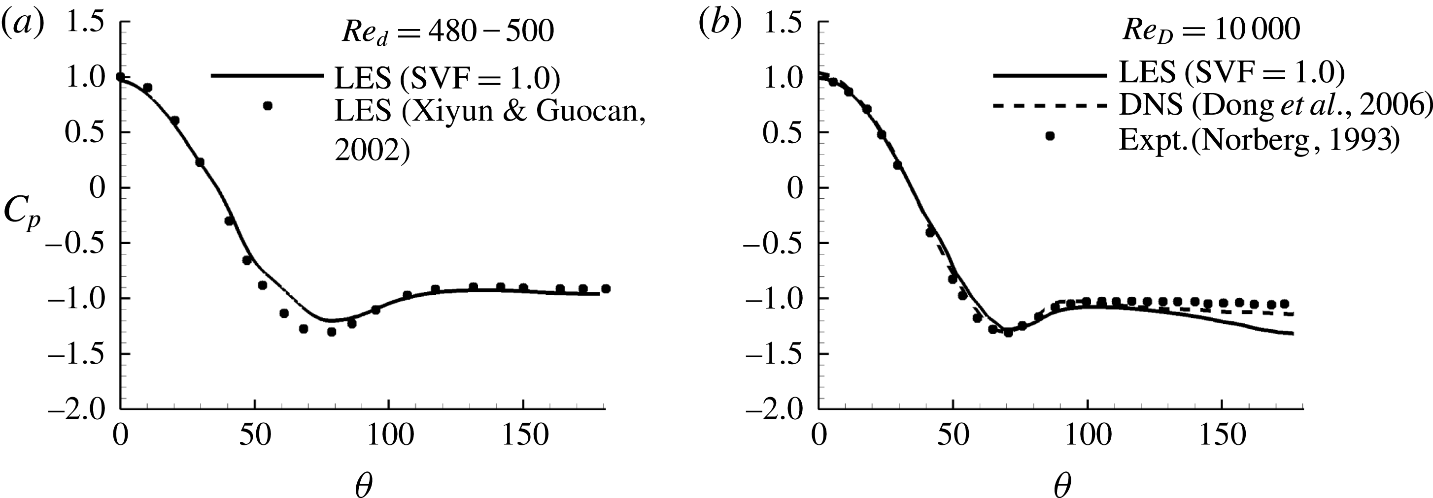
Distribution of pressure coefficient on an isolated cylinder as a function of the polar angle
 ${\it\theta}$
. (a) Small cylinder of diameter
 $d$
. Present results for
 $\mathit{Re}_{d}=480$
(solid line) are compared with LES of Xiyun & Guocan (Reference Xiyun and Guocan2002) (symbols) for
 $\mathit{Re}_{d}=500$
. (b) Large cylinder of diameter
 $D$
(
 $\text{SVF}=1.0$
). Present results for
 $\mathit{Re}_{D}=10\,000$
(solid line) are compared with DNS of Dong et al. (Reference Dong, Karniadakis, Ekmekci and Rockwell2006) (dashed line) for
 $\mathit{Re}_{D}=10\,000$
and experiment of Norberg (Reference Norberg1993) (symbols) for
 $\mathit{Re}_{D}=8000$
.

After the solution became statistically steady, statistics were collected over a time interval corresponding to approximately
 $50D/U$
. We checked that this time interval was long enough to obtain converged first- and second-order statistics and dominant frequencies in the velocity power spectra.
Most of the simulations were conducted with
 $\mathit{Re}_{D}=10\,000$
and
 $d=0.048D$
. Simulations with
 $d=0.048D$
and
 $\text{SVF}=0.023$
, 0.05, 0.1 and 0.2 are used to study the effect of the SVF of the porous cylinder on the flow. Results are also compared with the limiting case of a solid cylinder of diameter
 $D$
(case
 $\text{SVF}=1.0$
in table 1). Although most vegetated canopies generally have
 $\text{SVF}<0.08$
, higher values of the SVF can sometimes occur (Jamali, Zhang & Nepf Reference Jamali, Zhang and Nepf2008). Values of the SVF as high as 0.45 have been reported in mangroves with mean trunk diameters in the range
 $d=4{-}9~\text{cm}$
(Furukawa, Wolanski & Mueller Reference Furukawa, Wolanski and Mueller1997). Besides
 $d/D$
, the other relevant non-dimensional length scale is
 $1/(aD)$
, where
 $aD$
is the non-dimensional frontal area per unit volume (
 $aD=\text{SVF}(D/d)4/{\rm\pi}$
for circular cylinders). In the present simulations,
 $aD$
was varied between 0.61 and 5.44, which is within the range (
 $0.09<aD<8$
) of values in the experimental study of Zong & Nepf (Reference Zong and Nepf2012). The effect of the solid cylinder diameter is investigated by comparing the
 $\text{SVF}=0.2$
case (
 $N=89$
) with a simulation conducted with the same SVF but with solid cylinders of diameter
 $2d$
(
 $N=21$
,
 $\mathit{Re}_{d}=960$
). The latter simulation is denoted case
 $\text{SVF}=0.2(2\mathit{d})$
. Comparison of cases
 $\text{SVF}=0.2(2\mathit{d})$
and
 $\text{SVF}=0.1$
allows study of the effect of varying the SVF while maintaining
 $aD$
constant.
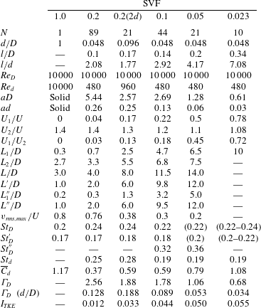
Main geometrical and flow variables of the test cases (
 $N$
is the number of cylinders in the array;
 $d$
is the diameter of the solid cylinders;
 $D$
is the diameter of the circular array;
 $l$
is the average distance between the rigid cylinders;
 $\mathit{Re}_{D}=UD/{\it\nu}$
,
 $\mathit{Re}_{d}=Ud/{\it\nu}$
;
 ${\it\nu}$
is the molecular viscosity;
 $aD$
is the non-dimensional frontal area per unit volume for the array;
 $U_{1}$
is the centreline streamwise velocity at the upstream end of the steady wake region;
 $U_{2}$
is the maximum streamwise velocity of the flow on the sides of the array;
 $L_{1},L_{1}^{\prime \prime }$
are estimates of the steady wake length;
 $L,L^{\prime },L^{\prime \prime }$
are estimates of the total wake length;
 $L_{2}=L-L_{1}$
;
 $v_{rms,max}$
is the maximum of the r.m.s. of the lateral velocity along the centreline;
 $\mathit{St}_{D}$
is the Strouhal number defined with
 $U$
and
 $D$
corresponding to the most energetic frequency in the wake of the (porous) cylinder;
 $\mathit{St}_{D}^{\prime }$
is the Strouhal number defined with
 $U_{2}$
and
 $D$
corresponding to the most energetic frequency in the wake of the (porous) cylinder;
 $\mathit{St}_{D}^{\prime \prime }$
is the Strouhal number defined with
 $U$
and
 $D$
corresponding to the second most energetic frequency in the wake present in cases when the von Karman vortex street is suppressed;
 $\mathit{St}_{d}$
is the Strouhal number defined with
 $U$
and
 $d$
corresponding to the main shedding frequency of wake billows behind the cylinders in the array;
 $\overline{C}_{d}$
is the mean solid cylinder streamwise drag coefficient;
 ${\it\Gamma}_{D}=\overline{C}_{d}\,aD/(1-\text{SVF})$
is a combined drag parameter for the array;
 $I_{TKE}$
is the integral of the turbulent kinetic energy over the porous cylinder region and a region extending 1.5D behind it).

Additional simulations of flow past an isolated solid cylinder with
 $d=0.048D$
were conducted. Results are reported for the simulation in which the spatial and temporal resolutions of the flow were sufficient to obtain good agreement with the available experimental data. For this case,
 $\mathit{Re}_{d}=\mathit{Re}_{D}=480$
and the resolution of the flow around the solid cylinder was the same as the one employed around the cylinders in the array for the porous cylinder cases. Figure 2(a) compares the distribution of the pressure coefficient on the cylinder,
 $Cp({\it\theta})=(p-p_{0})/{\it\rho}U^{2}$
(
 ${\it\rho}$
is the density,
 $p$
is the pressure on the cylinder,
 $p_{0}$
is the reference pressure away from the cylinder), predicted by the present LES results for
 $\mathit{Re}_{d}=480$
with that given by the LES of Xiyun & Guocan (Reference Xiyun and Guocan2002) for
 $\mathit{Re}_{d}=500$
. The agreement is satisfactory. The mean streamwise drag coefficient predicted by the present LES was 1.25, which is close to the value (1.2) reported in experiments (Munson et al.
Reference Munson, Okiishi, Huebsch and Rothmayer2012). The non-dimensional dominant shedding frequency of the wake billows was
 $\mathit{St}_{D}=fD/U=0.205$
(
 $f$
is the dimensional frequency), which is very close to experimental values determined at similar cylinder Reynolds numbers (Zdravkovich Reference Zdravkovich1997). Figure 2(b) presents a similar comparison for the case
 $\text{SVF}=1~(\mathit{Re}_{D}=10^{4})$
. The distribution of
 $Cp$
given by LES is close to that predicted by the DNS of Dong et al. (Reference Dong, Karniadakis, Ekmekci and Rockwell2006) performed for
 $\mathit{Re}_{D}=10^{4}$
and the experiments of Norberg (Reference Norberg1993, Reference Norberg2003) conducted with
 $\mathit{Re}_{D}=8000$
. The predicted value of the time-averaged streamwise drag coefficient was 1.17. This compares well with values predicted by DNS (1.11–1.21) and experiment (1.29). The values of
 $\mathit{St}_{D}$
predicted by the present LES, DNS and experiment were 0.205, 0.195–0.209 and 0.202 respectively. The length of the recirculation region measured in the mean flow by the present LES, DNS and experiment was 0.72, 0.8–0.82 and 0.78 respectively.
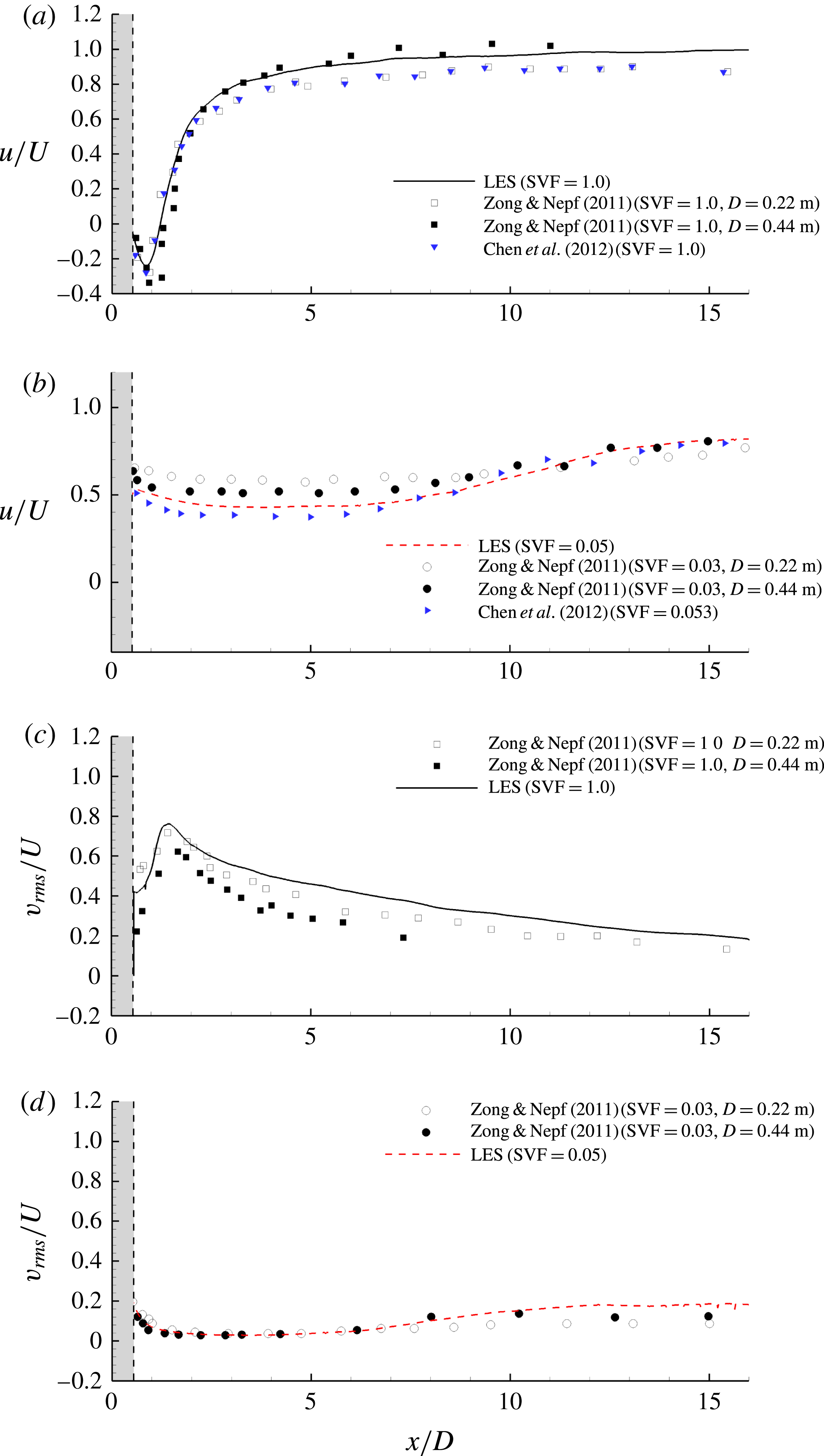
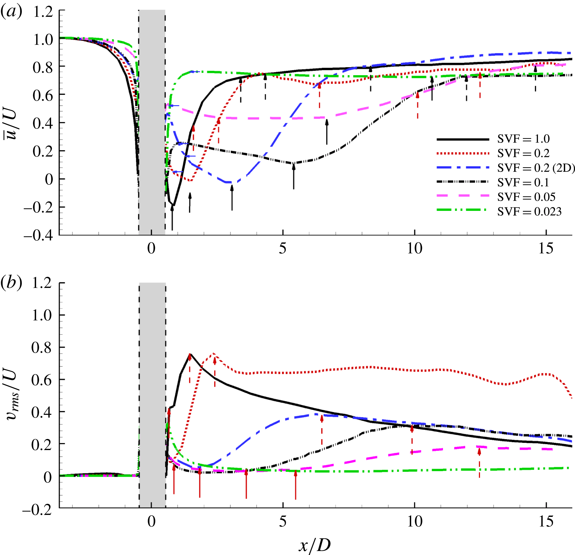
Figure 3 shows validation results for the simulations conducted with
 $\mathit{Re}_{D}=10\,000$
,
 $\text{SVF}=1.0$
(solid cylinder) and
 $\text{SVF}=0.05$
(see also table 1). The numerical predictions of the longitudinal profiles of the streamwise velocity,
 $\overline{u}/U$
, and the r.m.s. of the lateral velocity,
 $v_{rms}/U$
, along the centreline of the solid/porous cylinder are compared with the experimental measurements of Zong & Nepf (Reference Zong and Nepf2011) and Chen et al. (Reference Chen, Ortiz, Zong and Nepf2012). Results are included from two sets of experimental measurements conducted by Zong & Nepf (Reference Zong and Nepf2011) with different values of
 $D$
. The comparison for the solid cylinder case (figure 3
a) shows that the predicted centreline velocity is situated in between the two sets of experimental data measured by Zong & Nepf (Reference Zong and Nepf2011). The values of
 $v_{rms}/U$
along the centreline are slightly overpredicted by the numerical simulation (figure 3
c). One reason is the different level of background turbulence in the simulation, which was conducted with no resolved turbulence, and experiments. A direct comparison for the porous cylinder cases is not possible given the fact that the flow and turbulence structure through the array and in its wake are not only a function of the SVF, but also of other flow and geometrical parameters like the Reynolds number,
 $d/D$
, the mean drag coefficient for the array, the arrangement of the cylinders in the array, the level of turbulence in the incoming flow, etc. Still, the agreement between the numerical predictions of
 $\overline{u}/U$
and
 $v_{rms}/U$
for
 $\text{SVF}=0.05$
and the experiments conducted for
 $\text{SVF}=0.03$
by Zong & Nepf (Reference Zong and Nepf2011) and
 $\text{SVF}=0.053$
by Chen et al. (Reference Chen, Ortiz, Zong and Nepf2012) is quite good (figure 3
b,d). Chen et al. (Reference Chen, Ortiz, Zong and Nepf2012) did not report measurements of
 $v_{rms}/U$
.
Longitudinal profiles of the streamwise velocity,
 $\overline{u}/U$
(a,b), and the r.m.s. of the lateral velocity,
 $v_{rms}/U$
(c,d), measured along the centreline,
 $y/D=0$
. The grey region denotes the porous cylinder. Panels (a) and (c) show the comparison between the simulations and the experiments of Zong & Nepf (Reference Zong and Nepf2011) and Chen et al. (Reference Chen, Ortiz, Zong and Nepf2012) for the solid cylinder (
 $\text{SVF}=1$
) case. Panels (b) and (d) show the comparison between the simulation (case
 $\text{SVF}=0.05$
) and the experiments of Zong & Nepf (Reference Zong and Nepf2011) and Chen et al. (Reference Chen, Ortiz, Zong and Nepf2012) performed for
 $\text{SVF}=0.03$
and
 $\text{SVF}=0.053$
respectively. The two sets of experimental data from Zong & Nepf (Reference Zong and Nepf2011) correspond to different diameters of the porous cylinder (
 $D=0.22~\text{m}$
and
 $D=0.44~\text{m}$
).

3. Mean flow and turbulence statistics
Figure 4 compares the mean flow structure within and close to the porous cylinder for two simulations with different values of the SVF. In the first case, the SVF of the porous cylinder is sufficiently high (
 $\text{SVF}=0.2$
) such that wake-to-cylinder interactions are important and a significant part of the approaching flow is diverted laterally as it approaches the upstream face of the porous cylinder. In the second case, the SVF is sufficiently low (
 $\text{SVF}=0.023$
) such that the wake-to-cylinder interactions are weak and most of the incoming flow is advected through the porous cylinder. As will be discussed later, the former case corresponds to the regime where the von Karman vortex street forms, while the latter case corresponds to the regime where no vortex street forms past the porous cylinder.
Visualization of mean flow structure for cases with high (
 $\text{SVF}=0.2$
, a–c) and low (
 $\text{SVF}=0.023$
, d–f) volume fractions of solids: (a,d) pressure
 $\overline{p}/{\it\rho}U^{2}$
within the porous cylinder; (b,e) vertical vorticity magnitude
 $\overline{{\it\omega}}_{z}D/U$
within the porous cylinder; (c,f) vertical vorticity magnitude
 $\overline{{\it\omega}}_{z}D/U$
in the wake of the porous cylinder.

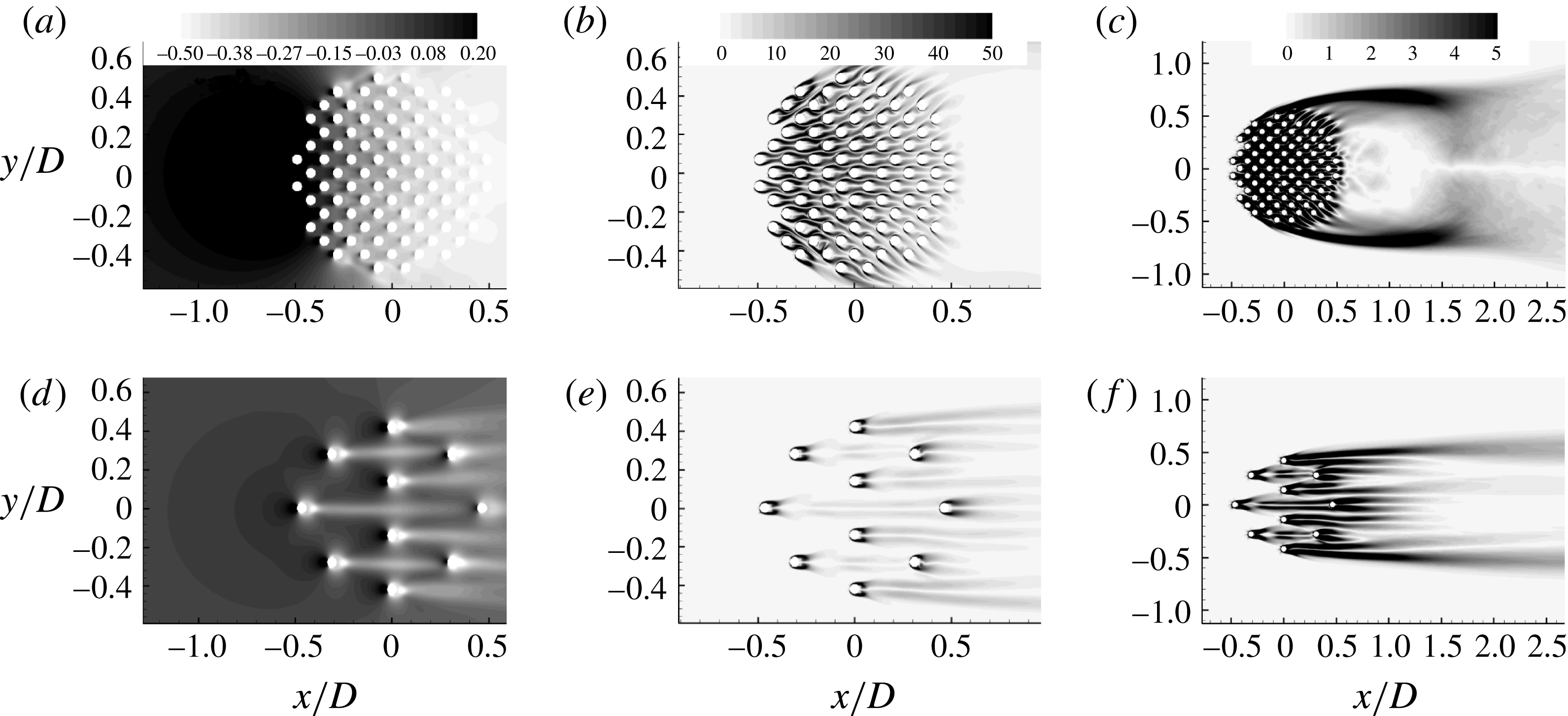
The bleeding flow through the porous cylinder is much weaker in the
 $\text{SVF}=0.2$
case because of the strong adverse pressure gradients induced by the solid cylinders directly exposed to the incoming flow and by those situated immediately behind. A continuous region of high pressure forms around the upstream face of the porous cylinder, similar to what is observed for a solid cylinder (figure 4
a, d). This is the main reason why a significant fraction of the incoming flow is diverted laterally, as also observed from the orientation of the SSLs on the solid cylinders directly exposed to the incoming flow (figure 4
b, e). By contrast, in the
 $\text{SVF}=0.023$
case, no noticeable increase of the pressure is observed around the upstream face of the porous cylinder, while the pressure is strongly amplified around the upstream face of all solid cylinders directly exposed to the flow. Moreover, the SSLs on all the solid cylinders are oriented fairly parallel to the streamwise direction, which means that the direction of the bleeding flow through the porous cylinder remains parallel to the incoming flow. This is not the case in the
 $\text{SVF}=0.2$
simulation where, away from the centreline, the bleeding flow has a strong lateral component. A significant part of the bleeding flow is diverted laterally towards the SSLs of the porous cylinder. Moreover, the drag induced by the cylinders reduces the speed of the bleeding flow. As a result, the SSLs are relatively weak for the solid cylinders situated in the region with
 $x/D\geqslant 0$
. Meanwhile, in the region with
 $x/D<0$
, the SSLs of the solid cylinders extend until the solid cylinders situated behind them, which suggests strong cylinder-to-wake interactions in this region.
Strong SSLs form on the sides of the porous cylinder for the case with a relatively high SVF (figure 4
c, f,
 $\text{SVF}=0.2$
). This is expected given the strong lateral diversion of the incoming flow approaching the porous cylinder and the small velocity of the bleeding flow exiting the back of the porous cylinder. What is less expected is that SSLs are also detected on the sides of the porous cylinder in the
 $\text{SVF}=0.023$
case. This is because the drag induced by the solid cylinders reduces the velocity of the bleeding flow behind the porous cylinder, close to the centreline (
 $U_{1}=0.78U$
, see table 1 for exact definition of
 $U_{1}$
) compared with the maximum streamwise velocity of the flow on the sides of the cylinder (
 $U_{2}$
), which is only slightly larger than the incoming flow velocity (
 $U_{2}\approx 1.08U$
for
 $\text{SVF}=0.023$
, see table 1). This difference explains the formation of fairly strong SSLs originating from the two solid cylinders situated at the lateral extremities of the porous cylinder. Therefore, porous cylinders can develop well-defined SSLs even for cases when the von Karman vortex sheet is not observed. The consequence of this important result will be discussed later.
Effect of the volume fraction of solids and relative cylinder size,
 $d/D$
, on the mean flow and turbulence structure: (a) the t.k.e.,
 $k/U^{2}$
, within the (porous) cylinder; (b) the t.k.e.,
 $k/U^{2}$
, in the wake of the (porous) cylinder; (c) 2D streamlines and mean streamwise velocity,
 $\overline{u}/U$
, visualizing mean flow in the wake of the (porous) cylinder. The solid black and dashed blue arrows pointing upwards show the ends of the steady wake region and total wake region respectively. The end of the steady wake region is defined as the location where the mean streamwise velocity along the centreline reaches a minimum in the wake of the porous cylinder. The end of the total wake region is defined as the location where the streamwise gradient of the mean streamwise velocity along the centreline becomes negligible (see also the discussion of figure 21). The two vertical arrows pointing downwards in panel (
 $c$
) show the start and end of the recirculation bubble at the back of the porous cylinder.

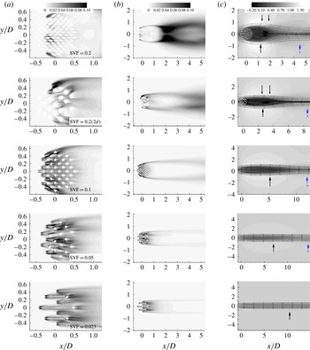
Information on the distribution of the turbulent kinetic energy (t.k.e.) through and immediately downstream of the circular array of cylinders is of particular importance for cases where the cylinders are organic (plant stems). The presence of regions of high t.k.e. inside and close to the back of the array has a direct consequence on nutrient availability for the plants in the array and on the amount of suspended sediment present in the water column inside the array region. It also means that the unsteady component of the drag force acting on the individual plant stems in regions of high t.k.e. is larger. In the case of flexible vegetation, this will affect the movement of the plant stems. Figure 5(a) shows that the t.k.e.,
 $k/U^{2}$
, generated by the solid cylinders increases monotonically with decrease in the SVF from 0.2 to 0.023. This is confirmed by the variation of the integral of the t.k.e. over the porous cylinder and a region extending 1.5D behind it,
 $I_{TKE}$
(table 1). The SSLs of the porous cylinder were excluded from the calculation of
 $I_{TKE}$
. The main contributor to the t.k.e. is the movement of the SSLs of the solid cylinders and the shedding of large-scale eddies behind them (see supplementary movie_2 available at http://dx.doi.org/10.1017/jfm.2015.321). For large values of the SVF, the SSLs of many of the solid cylinders extend until the solid cylinders situated behind them, which impedes the formation and shedding of strong vortices in the wakes of the solid cylinders. The t.k.e. is relatively low in the downstream half of the porous cylinder because the strength of the bleeding flow decreases significantly with
 $x$
due to the reasons discussed earlier. For
 $\text{SVF}\leqslant 0.1$
, the distance between the solid cylinders is sufficiently high to allow shedding of wake vortices behind most of the cylinders, and the bleeding flow is relatively strong inside the porous cylinder. This explains why the region of high t.k.e. approximately corresponds to the spatial extent of the porous region. As the SVF is further decreased, the strength of the bleeding flow increases and strong vortex shedding is observed even for the solid cylinders situated at the back of the porous cylinder. This is why the region of high t.k.e. includes part of the steady wake region. For very low values of the SVF (e.g.
 $\text{SVF}=0.023$
), the wakes of the cylinders directly exposed to the incoming flow resemble the wake past an isolated cylinder. A further lowering of the SVF is expected to result in a decay of
 $I_{TKE}$
, as for very low SVF values the wake-to-cylinder interactions should become negligible and
 $I_{TKE}$
should become proportional to the number of solid cylinders in the array. Based also on results obtained for an isolated rigid cylinder (see the discussion of figure 2
a), we estimate that this will happen for
 $\text{SVF}<0.01$
.
Figure 5(b) shows that for high SVF cases, the largest amplification of the t.k.e. occurs towards the end of the steady wake region, where the interaction between the SSLs of the porous cylinder results in the formation of billow vortices (e.g.
 $2\leqslant x/D\leqslant 3$
for
 $\text{SVF}=0.2$
). As opposed to the case of a solid cylinder where the recirculation bubbles touch the back of the cylinder, for porous cylinders the recirculation bubbles, if present, form close to the end of the steady wake region (figure 5
c). No recirculation bubbles are observed for
 $\text{SVF}\leqslant 0.1$
in figure 5(c). The advection of vortex-tube-like vortical eddies is the main mechanism responsible for the amplification of the t.k.e. inside the SSLs of the porous cylinder (figure 5
b and supplementary movie_1). The t.k.e. levels inside the SSLs decay with the decay in the SVF, but the amplification of the t.k.e. inside the SSLs is noticeable even for
 $\text{SVF}=0.023$
.
The effect of doubling the cylinder diameter while keeping the SVF constant is to increase
 $I_{TKE}$
by approximately 250 %. The reason is that the larger spacing between the cylinders allows the shedding of more energetic eddies. This is especially the case for the cylinders situated in the downstream half of the porous cylinder. The other effect of doubling
 $d/D$
is to increase the length of the steady wake region and the size of the main recirculation bubble, and to generate two smaller symmetrical bubbles at the back of the porous cylinder (figure 5
c). The effect of doubling the cylinder diameter while keeping
 $aD$
constant (compare cases
 $\text{SVF}=0.2(2\mathit{d})$
and
 $\text{SVF}=0.1$
) is to decrease
 $I_{TKE}$
by approximately 30 % and to decrease the length of the steady wake region,
 $L_{1}/D$
, by approximately 50 % (table 1 and figure 5
c).
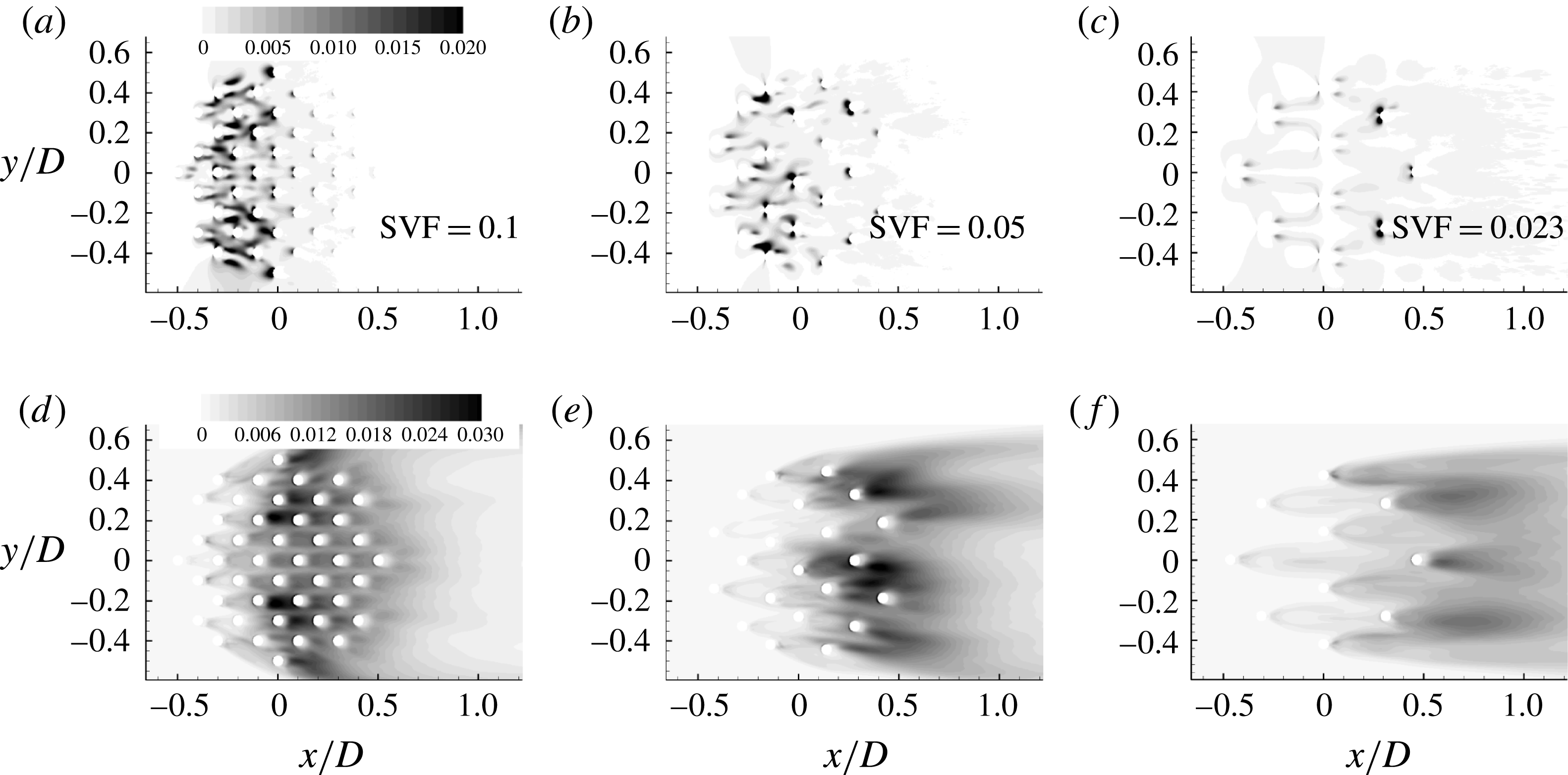
The distributions of the mean pressure fluctuations,
 $\overline{{p^{\prime }}^{2}}/{\it\rho}^{2}U^{4}$
, in figure 6(a–c) allow one to better understand the effect of lowering the SVF on the level of flow turbulence within the porous region. Large values of
 $\overline{{p^{\prime }}^{2}}$
on the upstream side of the solid cylinders are a good indicator of strong wake-to-cylinder interactions, while high
 $\overline{{p^{\prime }}^{2}}$
values downstream of the solid cylinders are a good indicator of shedding of energetic eddies in the wakes of these cylinders. For
 $\text{SVF}=0.1$
, high values of
 $\overline{{p^{\prime }}^{2}}$
are observed both in front of and behind the solid cylinders situated in the
 $-0.3\leqslant x/D\leqslant 0$
region. As the SVF decreases, the cylinders situated close to the upstream face of the porous cylinder become a main source of turbulence via shedding of strongly coherent wake billows, while most of the cylinders situated behind the upstream face of the porous cylinder are subject to large pressure fluctuations generated by the passage of eddies shed from the upstream cylinders.
Effect of the volume fraction of solids on the distribution of the mean pressure fluctuations,
 $\overline{{p^{\prime }}^{2}}/{\it\rho}^{2}U^{4}$
(a–c), and the mean vertical velocity fluctuations,
 $\overline{{w^{\prime }}^{2}}/U^{2}$
(d–f), within and downstream of the porous cylinder.

An important question is the effect of the SVF on the transition to 3D inside the porous cylinder. This is very relevant for practical applications in vegetated canopies where one is interested in characterizing the nutrient transport inside the porous patch. Given that the present simulations were performed without a no-slip bottom boundary, the present findings are relevant for the canopy region situated away from the bed surface. In the absence of 3D turbulence, the vertical transport is negligible. For
 $\text{SVF}=0.1$
, the region of high mean vertical velocity fluctuations,
 $\overline{{w^{\prime }}^{2}}$
, coincides with the porous cylinder region except for its upstream part (figure 6
d–f). This is because it takes some distance for the secondary 3D instabilities to grow and for vortex stretching acting on the quasi-2D eddies shed by the most upstream solid cylinders to generate a flow with a large 3D eddy content. As the SVF decreases to 0.05, the region of high
 $\overline{{w^{\prime }}^{2}}$
has approximately the same length as for
 $\text{SVF}=0.1$
, but occupies only the downstream half of the porous region. For sufficiently low values of the SVF, the flow remains close to 2D within the porous cylinder and the region of high
 $\overline{{w^{\prime }}^{2}}$
is situated downstream of the porous cylinder (e.g. see results for
 $\text{SVF}=0.023$
in figure 6
d–f). For such cases, the only mechanism for vertical transport is due to the turbulence present in the incoming flow, which was not considered in the present simulations. However, this is expected to be a weaker contributor to the generation of 3D motions within the porous region compared with the 3D turbulence generated by the solid cylinders.
Effect of the volume fraction of solids on the distribution of the instantaneous vertical vorticity magnitude,
 ${\it\omega}_{z}D/U$
, in the wake of the porous cylinder. Here, (a)
 $\text{SVF}=1.0$
; (b)
 $\text{SVF}=0.2$
; (c)
 $\text{SVF}=0.05$
; (d)
 $\text{SVF}=0.023$
. The black arrows show the streamwise extent of the SSL based on the mean flow vertical vorticity magnitude,
 $\overline{{\it\omega}}_{z}D/U$
, distributions and a threshold value
 $\overline{{\it\omega}}_{z}D/U=3$
(see also figure 4
c, f). For the case
 $\text{SVF}=0.05$
, the SSL ends at
 $x/D\approx 7$
.

4. Vortical structures in the instantaneous flow fields
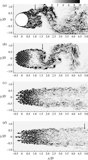
Figure 7 and supplementary movie_1 use vertical vorticity contours to visualize the vortical structure of the instantaneous flow in an
 $x{-}y$
plane. For
 $\text{SVF}=0.2$
, the wake structure is qualitatively similar to that observed for a solid cylinder (
 $\text{SVF}=1.0$
). The main difference is that the SSLs are longer so the wake billows form away from the cylinder (e.g. around
 $x/D=1.5$
for
 $\text{SVF}=0.2$
) rather than at the back of the cylinder. The coherence of the vortex tubes shed in the SSLs of the porous cylinder with
 $\text{SVF}=0.2$
is significantly larger than that observed in the
 $\text{SVF}=1.0$
case. This is because the solid cylinders situated on the circumference of the porous cylinder, close to the region where the SSL on the porous cylinder originates, act as a source of large-scale quasi-2D turbulence for the SSLs (see supplementary movie_1 and movie_2).
As the SVF is further decreased, the SSLs get longer and the strength of the bleeding flow at the back of the cylinder increases sufficiently such that the lateral movement of the end of one of the SSLs towards the other SSL is impeded. Once this happens, the formation and shedding of wake billows with alternate directions of rotation is suppressed. For example, this is the case for the simulation with
 $\text{SVF}=0.05$
(see figure 7
c and supplementary movie_1). Still, the downstream part of the SSLs contains large-scale eddies forming via merging of neighbouring eddies containing vorticity of the same sign, similar to the classical merging of co-rotating vortices observed in mixing layers. The size of these eddies is much larger than that of the vortex tubes present in the upstream part of the SSLs. The wake undergoes what is called a symmetric wake shedding (e.g. see supplementary movie_1,
 $\text{SVF}=0.05$
), to be contrasted with the antisymmetrical wake shedding which results in the formation of the von Karman vortex street (e.g. see supplementary movie_1,
 $\text{SVF}=0.2$
). The symmetric wake shedding is generally observed when the interaction of the SSLs forming on the sides of an obstruction is impeded. Classical examples are flow past solid cylinders in which a sufficiently long streamwise oriented plate is mounted along the cylinder centreline at its back and shallow flow past a solid cylinder with a deep scoured bed (Kirkil, Constantinescu & Ettema Reference Kirkil, Constantinescu and Ettema2009; Kirkil & Constantinescu Reference Kirkil and Constantinescu2010).
Separated shear layers form on the sides of the porous cylinder even for
 $\text{SVF}=0.023$
. For this case, the bleeding flow behind the back of the porous cylinder is quite strong and contains a wide range of turbulent eddies shed by the solid cylinders. Even so, the eddies inside the SSLs maintain their coherence for a much longer streamwise distance compared with the wake vortical eddies situated closer to the centreline (figure 7
d). The reason for this is the additional mean shear acting on the SSLs eddies as they are advected downstream. The mean shear is due to the mean velocity difference across the SSL, which is proportional to
 $U_{2}{-}U_{1}$
(table 1). Only for very low values of the SVF, where the difference between
 $U_{1}$
and
 $U_{2}$
is not significant, will SSLs not form on the sides of the porous cylinder.
The value of the SVF also affects the vortical structure of the flow inside the porous cylinder. For high values of the SVF, the mean distance between neighbouring cylinders is small and it is very common for the SSLs from one solid cylinder to reach one of the solid cylinders situated behind it (e.g. the case
 $\text{SVF}=0.2$
in figure 7
b and supplementary movie_2). As a result, the natural interaction of the SSLs is impeded. Although the SSLs of most of the cylinders in the array are unsteady and patches of vorticity sometimes detach from their ends, no regular wake billows form. For
 $\text{SVF}\leqslant 0.05$
, the distance among the neighbouring cylinders is large enough such that the shedding of billows in the wake of the cylinders directly exposed to the flow (e.g. the region with
 $x/D\leqslant 0$
in figure 7
c and supplementary movie_2) is quasi-regular. The shedding of wake billows from the downstream solid cylinders is strongly disturbed by the vortical eddies passing in the vicinity of these cylinders or hitting them (see supplementary movie_2 for
 $\text{SVF}=0.05$
). For even lower values of the SVF (e.g. the case
 $\text{SVF}=0.023$
in figure 7
d), the shedding from most of the cylinders resembles the regular shedding observed past isolated cylinders.
The dominant non-dimensional wake shedding frequency in the cases
 $\text{SVF}=0.2$
and
 $0.2(2d)$
is
 $\mathit{St}_{D}=0.24$
, which shows that the shedding frequency is mainly a function of the SVF and less a function of
 $d/D$
or
 $aD$
. This value is approximately 20 % larger than the one observed for the solid cylinder case (
 $\mathit{St}_{D}=0.2$
). As the SVF decreases to 0.1,
 $\mathit{St}_{D}$
decreases to 0.22. Interestingly, velocity and drag power spectra show that a frequency component in the range
 $\mathit{St}_{D}=0.2{-}0.24$
remains very energetic even for cases (
 $\text{SVF}=0.05$
and
 $\text{SVF}=0.023$
) where the von Karman vortex street is not observed (e.g. see the discussion of figure 15 below). This result is consistent with the measurements of Zong & Nepf (Reference Zong and Nepf2012) which also detected a dominant wake frequency close to 0.2 for cases where the von Karman vortex street did not form. No explanation was provided for this phenomenon. Examination of animations for the case
 $\text{SVF}=0.023$
showed that the two SSLs assume an undulatory shape. The
 $\mathit{St}_{D}=0.22{-}0.24$
frequency corresponds to the undulatory in-phase motions of the SSLs. This type of instability is sometimes observed between two parallel rows of vortices.
Table 1 also lists the dominant shedding frequency non-dimensionalized with the maximum velocity on the outer side of the SSLs,
 $U_{2}$
. This Strouhal number is denoted
 $\mathit{St}_{D}^{\prime }$
. For cases where the vortex street was present, Zong & Nepf (Reference Zong and Nepf2012) predicted values of
 $\mathit{St}_{D}^{\prime }$
in the range of 0.18–0.2. The present simulations predict
 $\mathit{St}_{D}^{\prime }=0.17{-}0.18$
. The scatter in the measured values of
 $\mathit{St}_{D}^{\prime }$
was larger for cases with a low SVF where the vortex street did not form (
 $\mathit{St}_{D}^{\prime }=0.14{-}0.23$
). For these cases, the present simulations predict
 $\mathit{St}_{D}^{\prime }=0.2$
. For cases with values of the SVF close to the threshold value at which the von Karman vortex street is suppressed, velocity power spectra in the wake revealed a second energetic frequency,
 $\mathit{St}_{D}^{\prime \prime }$
(like for
 $\mathit{St}_{D}$
,
 $U$
is used as the velocity scale). Its value is 0.32 for the case
 $\text{SVF}=0.1$
(the von Karman vortex street is present) and 0.36 for the case
 $\text{SVF}=0.5$
(the vortex street is absent). Animations of the vortical flow fields show that this frequency is associated with the formation of large vortical structures over the downstream part of the SSLs (e.g. see supplementary movie_1 for
 $\text{SVF}=0.05$
).
Figure 8 visualizes the coherent structures in the instantaneous flow fields using the
 $\unicode[STIX]{x1D64C}$
criterion (Dubief & Delcayre Reference Dubief and Delcayre2000). The quantity
 $\unicode[STIX]{x1D64C}$
is the second invariant of the resolved velocity gradient tensor (
 $\unicode[STIX]{x1D64C}=-0.5\;\partial u_{i}/\partial x_{j}\ast \partial u_{j}/\partial x_{i}(D^{2}/U^{2})$
). Positive
 $\unicode[STIX]{x1D64C}$
isosurfaces isolate areas where the strength of rotation overcomes the strain, making those surfaces eligible as vortex envelopes. The cylinder Reynolds number,
 $\mathit{Re}_{d}$
, was equal to or larger than 480 in all simulations with
 $\text{SVF}<1$
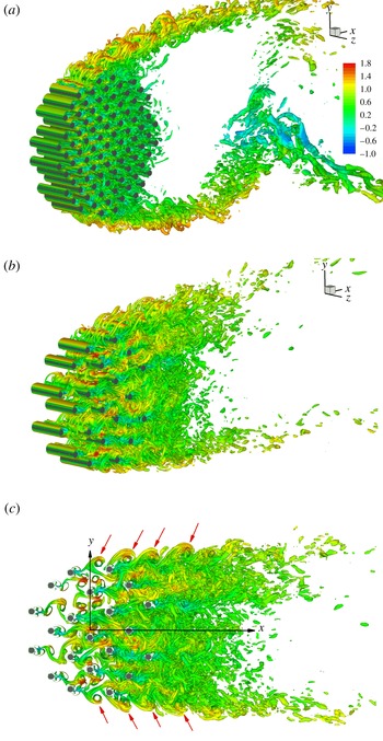
. Consistent with this, most of the 3D structures forming in the SSLs of the solid cylinders (e.g. the streamwise vortex pairs seen in figure 8(a,b) for the cylinders situated close to the lateral sides of the porous cylinder) correspond to fine-scale structures typical of mode B, according to the classification of Williamson (Reference Williamson1996). For cases with a high SVF (e.g. see figure 8
a), most of the large-scale energetic eddies within the SSLs of the porous cylinder are quasi-2D billows shed in the wake of the solid cylinders situated on the circumference of the porous cylinder, close to its lateral extremities. Similar to the classical case of flow past isolated solid cylinders, disturbances are induced along the cores of these parallel vortical eddies. The cores of the weaker ones are deformed and connect with the neighbouring ones to form an array of hairpin-like eddies whose legs contain streamwise vorticity. Eventually these legs evolve into finger-like structures connecting the larger spanwise vortical structures that are themselves subject to 3D stretching and straining. Moreover, the bleeding flow is oriented obliquely towards the SSLs of the porous cylinder. For these reasons, large-scale turbulence in the form of wake vortices from the cylinders in the array is fed into the upstream part of the SSLs, and these vortices are subject to strong 3D instabilities which force transition to turbulence over a relatively short distance.
Visualization of the coherent structures in an instantaneous flow field using the
 $\unicode[STIX]{x1D64C}$
criterion: (a)
 $\text{SVF}=0.2$
, 3D view; (b)
 $\text{SVF}=0.05$
, 3D view; (c)
 $\text{SVF}=0.05$
,
 $x{-}y$
view. The
 $\unicode[STIX]{x1D64C}$
isosurface (
 $\unicode[STIX]{x1D64C}=50$
) is coloured using the streamwise velocity
 $u/U$
. The red arrows point towards the large eddies (vortex tubes) generated in the SSLs of the porous cylinder. Only part of the computational domain is shown, as the vertical length is
 $D$
.

The other difference from the case of a solid cylinder (
 $\text{SVF}=1$
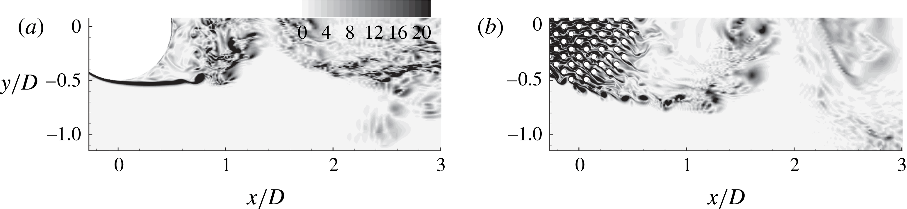
) is that the eddies advected into the SSLs of a porous cylinder are much more energetic (e.g. see figure 9 which compares cases with
 $\text{SVF}=1$
and 0.2). This is because the Kelvin–Helmholtz instabilities need a relatively long distance to develop into vortex tubes in the
 $\text{SVF}=1$
case. In the case of a porous cylinder, much more coherent vortical eddies are generated around the location where the SSLs separate from the porous cylinder. The solid cylinders situated close to each extremity of the porous cylinder are a major source of large-scale vortical eddies for the SSLs (see supplementary movie_2 for the case
 $\text{SVF}=0.2$
).
Distribution of the instantaneous vertical vorticity magnitude,
 ${\it\omega}_{z}D/U$
, visualizing the vortical structure of the SSL: (a)
 $\text{SVF}=1.0$
; (b)
 $\text{SVF}=0.2$
.

For cases with a low SVF (e.g. see figure 8
b for
 $\text{SVF}=0.05$
), the transition mechanism inside the SSLs of the porous cylinder remains essentially the same. As the lateral component of the bleeding flow close to the sides of the porous cylinder is weaker, the interactions between wake billows shed from the interior cylinders and the ones shed from the cylinders situated on the circumference of the porous cylinder are less strong. As shown in figure 8(c), most of the large-scale quasi-2D eddies injected into the SSLs in the
 $\text{SVF}=0.05$
case are generated only by two solid cylinders on each side of the porous cylinder. Due to the increase in the strength of the bleeding flow, the production of turbulence by mean shear inside the SSLs is less important for cases with a low SVF. Meanwhile, the larger strength of the bleeding flow and the higher values of the
 $l/d$
ratio create the conditions for the shedding of strongly coherent wake billows from the solid cylinders directly exposed to the flow for cases with a low SVF (figure 8
c and supplementary movie_2). Strong wake-to-cylinder interactions take place within the interior of the porous cylinder among these quasi-2D eddies which are approximately parallel to the axes of the cylinders. These interactions increase the flow three-dimensionality and eventually generate a strongly turbulent flow within the downstream half of the porous cylinder.
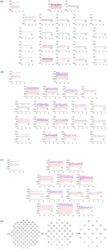
Variation of the drag coefficient,
 $C_{D}^{n}$
(blue solid line), and lift coefficient,
 $C_{L}^{n}$
(red dashed line), as a function of the non-dimensional time (
 $0\leqslant tU/D\leqslant 6$
) on the solid cylinders in the array (
 $n$
is the index of the solid cylinders). The inset at the top left shows the distributions of the drag and lift coefficients from a simulation of flow past an isolated solid cylinder with
 $d/D=0.048~(\mathit{Re}_{d}=480)$
: (a)
 $\text{SVF}=0.2$
; (b)
 $\text{SVF}=0.1$
; (c)
 $\text{SVF}=0.05$
. Panel (d) shows the relative position of the solid cylinders in the array and the cylinder index for the
 $\text{SVF}=0.2$
, 0.1 and 0.05 cases.

5. Non-dimensional drag/lift forces
5.1. Drag/lift coefficients of solid cylinders in the array
The effect of the coherent eddies and bleeding flow on the drag forces acting on the individual cylinders is discussed next. The lateral (
 $y$
) component of the drag force is referred to as the lift force. The streamwise component is simply referred to as the drag force. Figure 10 presents the temporal variation of the drag (
 $C_{D}^{n}=F_{x}^{n}/(0.5{\it\rho}U^{2}d)$
, where
 $F_{x}^{n}(t)$
is the drag force acting in the
 $x$
direction on the solid cylinder whose index in the array is
 $n$
) and lift (
 $C_{L}^{n}=F_{y}^{n}/(0.5{\it\rho}U^{2}d)$
) coefficients for some of the solid cylinders in the array. This information is especially relevant for vegetated patches containing flexible plant stems. Also shown are the distributions of
 $C_{D}^{n}$
and
 $C_{L}^{n}$
from a simulation of flow past an isolated solid cylinder with
 $d/D=0.048$
(
 $\mathit{Re}_{d}=480$
) for which the time-averaged values of the drag and lift coefficients are
 $\overline{C}_{D}^{n}=1.25$
and
 $\overline{C}_{L}^{n}=0$
and the most energetic mode of the power spectrum for the lift force has a non-dimensional frequency
 $\mathit{St}_{d}=0.205$
.
In the
 $\text{SVF}=0.2$
case (figure 10
a), there is no wake vortex shedding behind the first row of cylinders exposed to the flow, except for the cylinders (
 $n=83,88$
) situated very close to the lateral extremities of the porous cylinder which are exposed to the accelerating flow region on the sides of the porous cylinder. As a result, the drag and lift forces on the cylinders from which no wake vortices are shed (e.g.
 $n=42,57,70$
) are close to steady. The adverse pressure gradients associated with the porous cylinder slow down the flow approaching the porous region (see figure 4
a, d for
 $\text{SVF}=0.2$
). The main consequence is a reduction by approximately 40 % of
 $\overline{C}_{D}^{n}$
for most of the cylinders exposed to the incoming flow compared with the value predicted for an isolated cylinder. The velocity magnitude of the bleeding flow decreases with
 $x$
inside the porous region, especially close to the centreline of the porous cylinder. This is why
 $\overline{C}_{D}^{n}$
decreases with
 $x/D$
and reaches close-to-zero values for the cylinders situated at the back of the porous cylinder (e.g.
 $n=48$
, 63, 76, 87). Regular shedding of vortical eddies from the downstream part of the SSLs is observed starting with the third row of solid cylinders (see supplementary movie_2). The formation of these eddies is impeded by the presence of neighbouring cylinders which constrain the amplitude of the oscillatory movements of the SSLs. Consequently, for most of the cylinders situated away from
 $|y|/D=0.5$
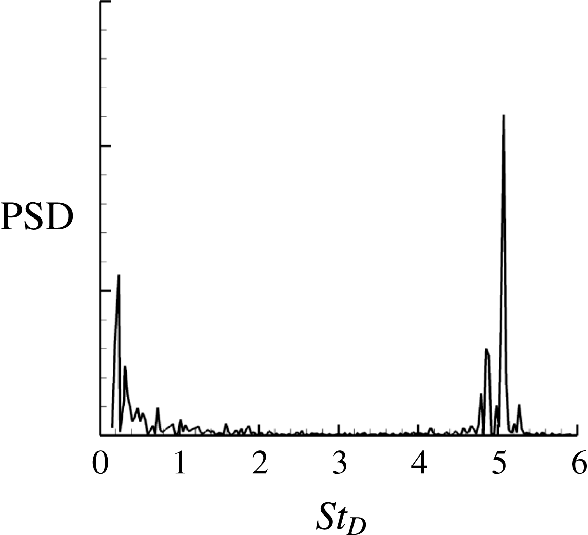
, the mean amplitude of the lift oscillations is much smaller than that for an isolated cylinder. For the most upstream cylinders which are subject to large-scale oscillations of the lift, the dominant frequency corresponds to
 $\mathit{St}_{d}\approx 0.25$
(figure 11). Due to the strong wake-to-cylinder interactions and the increase of the three-dimensionality of the bleeding flow, the velocity and lift force power spectra become broader for the cylinders situated in the region with
 $x/D\geqslant 0$
. An energetic frequency component is also observed around
 $\mathit{St}_{D}=0.24~(\mathit{St}_{d}\approx 0.01)$
in the power spectra of
 $C_{D}^{n}$
and
 $C_{L}^{n}$
for the cylinders situated close to the sides and the back of the porous cylinder (e.g. see figure 11). This component is induced by the formation and shedding of billow vortices in the wake of the porous cylinder.
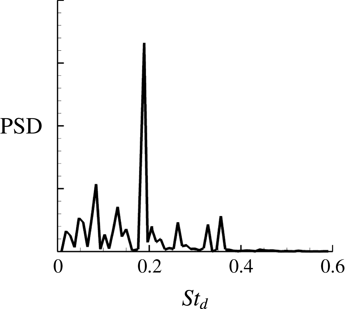
Power density spectrum of the lift coefficient,
 $C_{L}^{n}$
, for cylinder
 $n=89$
, case
 $\text{SVF}=0.2$
. The energetic frequency at
 $\mathit{St}_{D}=5.1~(\mathit{St}_{d}=0.25)$
is induced by shedding of vortices in the wake of the solid cylinder.

The
 $\text{SVF}=0.1$
case shown in figure 10(b) is representative of cases where
 $l/d$
is sufficiently high such that wake vortices can form behind the solid cylinders directly exposed to the incoming flow. Still, the SVF is sufficiently large such that a region of strong adverse pressure gradients forms around the upstream face of the porous cylinders, which slows down considerably the bleeding flow in the upstream part of the porous region. For these cylinders (e.g.
 $n=35$
, 26),
 $\overline{C}_{D}^{n}$
is smaller than the value predicted for an isolated cylinder and the mean amplitude of the lift oscillations is comparable to that predicted for an isolated cylinder. The lift oscillations are quasi-regular, with a dominant frequency of
 $\mathit{St}_{d}=0.19$
. The cylinders directly exposed to the accelerating flow on the sides of the porous cylinders (e.g.
 $n=40$
, 44) are characterized by strong lift and drag oscillations of larger amplitudes than those observed for an isolated cylinder. As opposed to the
 $\text{SVF}=0.2$
case, there is only a small decay of
 $\overline{C}_{D}^{n}$
with
 $x/D$
for the cylinders situated behind the ones exposed to the incoming flow. In the region of strong flow turbulence (figure 5
a) and strong wake-to-cylinder interactions within the porous cylinder, the mean amplitudes of the lift and drag fluctuations on the solid cylinders (e.g.
 $n=22$
, 27, 28, 36, 37, 41) are significantly larger than those predicted for an isolated cylinder. The mean amplitude of the
 $C_{D}^{n}$
and
 $C_{L}^{n}$
oscillations is smaller for the cylinders situated at the back of the porous region (
 $n=25$
, 29, 30, 38, 39, 43). As these cylinders are surrounded by turbulent flow, the power spectra of the forces acting on these cylinders display a wide range of energetic frequencies.
Decaying the SVF to 0.05 (figure 10
c) results in a larger number of cylinders that shed wake vortices whose coherence is comparable to that for an isolated cylinder. For the solid cylinders situated on the trajectory of wake vortices shed from the upstream cylinders (
 $n=11$
, 18, 19), the regular contact of the vortices advected from upstream with the cylinder surface can result in strong oscillations of the drag/lift forces. For some of these cylinders (e.g.
 $n=11$
), the mean drag force can be larger than that observed for an isolated cylinder. As the region where the flow becomes turbulent moves downstream with the decay in the SVF (figure 6
d–f), the power spectra of the drag/lift forces on most of the cylinders within the array contain a well-defined peak at
 $\mathit{St}_{d}=0.19$
(figure 12), which is induced by the quasi-regular vortex shedding of wake billows. Broader power spectra are observed only for some of the cylinders situated at the back of the porous region (
 $n=12$
, 15, 16). Such a spectrum is shown in figure 12.
Power density spectrum of the lift coefficient,
 $C_{L}^{n}$
, for cylinder
 $n=16$
, case
 $\text{SVF}=0.05$
.

Several important qualitative differences with the previous cases are observed once the SVF is sufficiently low (case
 $\text{SVF}=0.023$
) for the adverse pressure gradients induced by the porous cylinder to be negligible (figure 4
a, d) and for the mean velocity of the bleeding flow in the upstream part of the porous region to be close to the free-stream value,
 $U$
. For the cylinders directly exposed to the incoming flow (
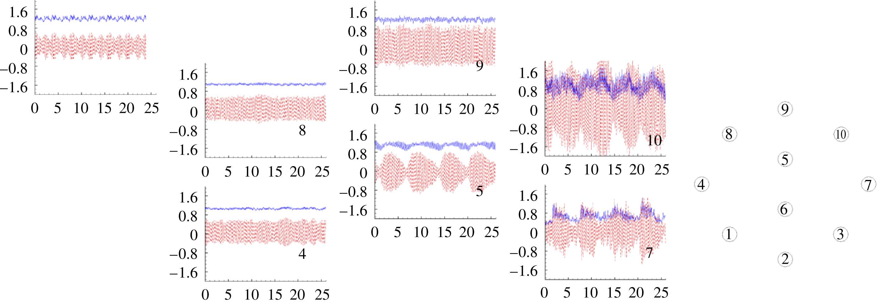
 $n=4$
, 8 in figure 13), the time histories of the lift/drag forces and the mean value of the drag force are very close to the values predicted for an isolated cylinder. The regular contact of wake vortices generated by an upstream cylinder with a cylinder situated along their paths can result in a large amplification of the mean amplitude of the lift force on the latter cylinder (e.g.
 $n=10$
). The absence of a broad spectrum of the drag/lift forces for all cylinders within the array is also expected, given that the transition to turbulence happens outside the porous region (case
 $\text{SVF}=0.023$
in figure 6
d–f).
Variation of the drag coefficient,
 $C_{D}^{n}$
(blue solid line), and lift coefficient,
 $C_{L}^{n}$
(red dashed line), as a function of the non-dimensional time (
 $0\leqslant tU/D\leqslant 25$
) on the solid cylinders in the array (
 $n$
is the index of the solid cylinders). Results are shown for the case
 $\text{SVF}=0.023$
. The inset at the top left shows the distributions of the drag and lift coefficients from a simulation of flow past an isolated solid cylinder with
 $d/D=0.048$
(
 $\mathit{Re}_{d}=480$
). The inset on the right side shows the relative position of the solid cylinders in the array and the cylinder index.

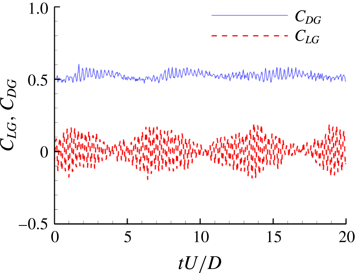
Temporal variation of the total drag coefficient,
 $C_{DG}$
(blue solid line), and total lift coefficient,
 $C_{LG}$
(red dashed line), of the porous cylinder for the case
 $\text{SVF}=0.023$
.

An interesting result is the presence of a very energetic low-frequency component (
 $\mathit{St}_{D}=0.22{-}0.24$
) in the time series of the drag and lift forces acting on the solid cylinders situated in the downstream part of the porous region. This frequency is not associated with large eddies that form and are advected into the SSLs of the porous cylinder, as the lift/drag forces on the
 $n=9$
cylinder situated in the region where the SSL originates are not subject to quasi-regular oscillations with
 $\mathit{St}_{D}=0.22{-}0.24$
. As discussed in the previous section, this frequency is present in velocity spectra at points located inside the wake of the porous cylinder and is associated with the in-phase undulatory motions of the SSLs of the porous cylinder. These undulatory motions and the low-frequency oscillations of the drag are induced by instabilities acting on the row of parallel vortices shed from the upstream cylinders that are directly exposed to the flow. The
 $n=5$
cylinder is not situated in the wake of an upstream cylinder but it is located in between the parallel rows of counter-rotating vortices shed from the
 $n=4$
and
 $n=8$
cylinders. The low-frequency component (
 $\mathit{St}_{D}=0.22{-}0.24$
) is also present in the time series and power spectra of the total drag (
 $C_{DG}=(\sum _{n=1}^{N}F_{x}^{n})/(0.5{\it\rho}U^{2}D)$
) and lift (
 $C_{LG}=(\sum _{n=1}^{N}F_{y}^{n})/(0.5{\it\rho}U^{2}D)$
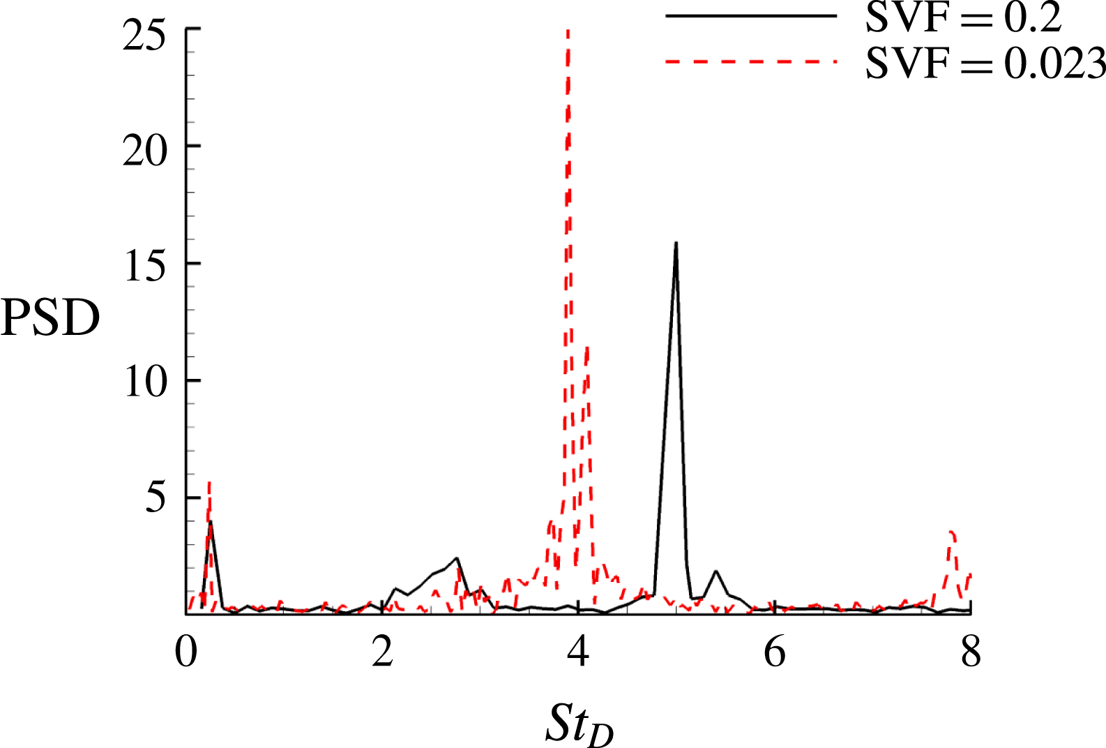
) coefficients (see figures 14 and 15 for
 $\text{SVF}=0.023$
which contain two peaks at
 $\mathit{St}_{D}=3.9~(\mathit{St}_{d}=0.19)$
and
 $\mathit{St}_{D}\approx 0.23$
). The time series of
 $C_{LG}$
for cases with a higher SVF (e.g. see figure 15 for
 $\text{SVF}=0.2$
) show that a low-frequency component corresponding to the dominant frequency in the wake of the porous region (e.g. the shedding frequency of counter-rotating vortices for cases when the von Karman vortex street is observed) is present, but this frequency (
 $\mathit{St}_{D}=0.24$
for
 $\text{SVF}=0.2$
) is less energetic than the dominant frequency associated with the vortex shedding past the solid cylinders in the array (
 $\mathit{St}_{D}=5.1$
for
 $\text{SVF}=0.2$
).
Power density spectra of the total lift coefficient of the porous cylinder,
 $C_{LG}$
, for the cases
 $\text{SVF}=0.2$
(black line) and
 $\text{SVF}=0.023$
(dashed red line). The main peak in the spectra corresponds to the main shedding frequency for the solid cylinders in the array (
 $\mathit{St}_{d}=$
0.25 for
 $\text{SVF}=0.2$
and
 $\mathit{St}_{d}=0.19$
for
 $\text{SVF}=0.023$
as
 $\mathit{St}_{d}=\mathit{St}_{D}/(D/d)$
).

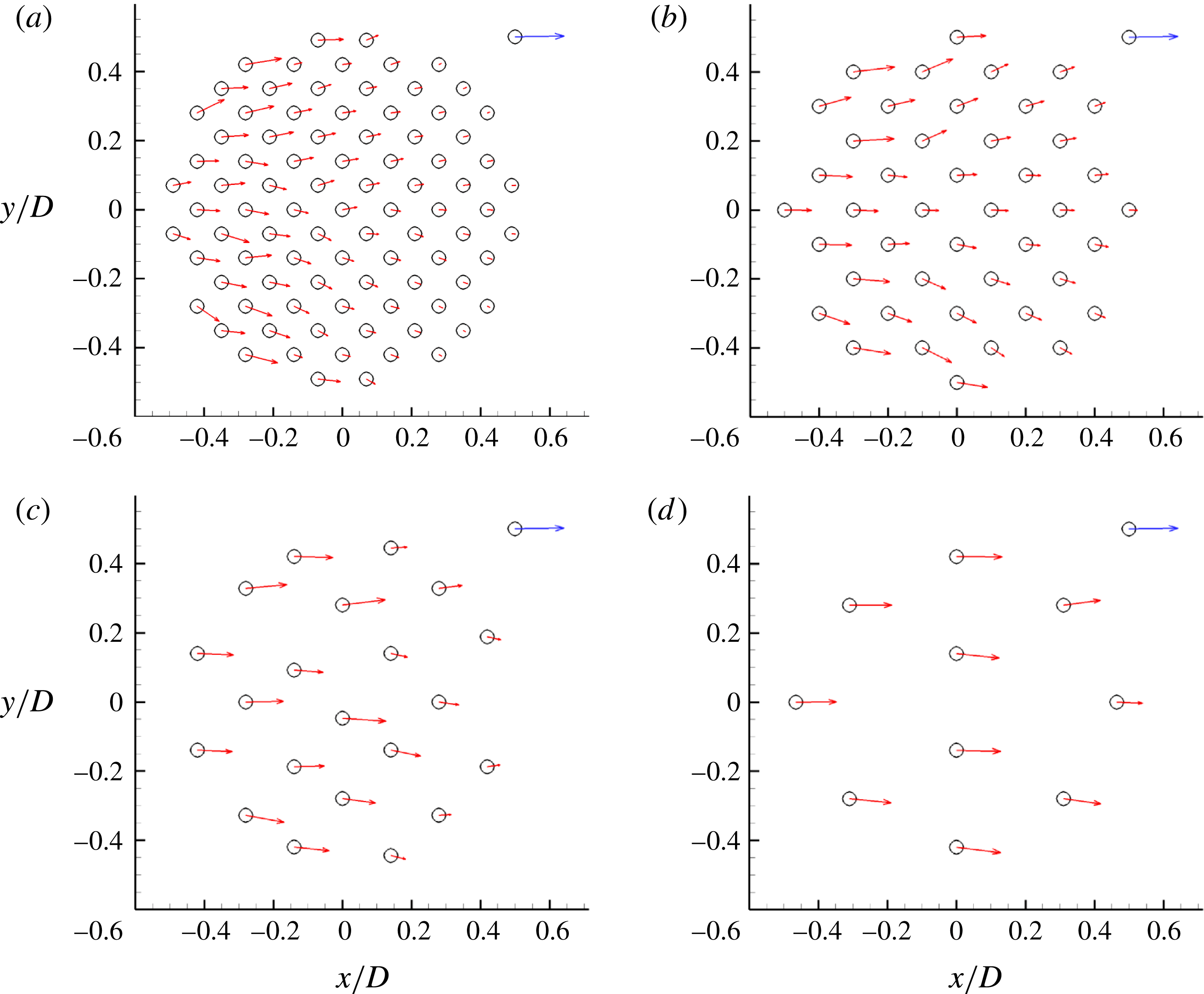
The time-averaged non-dimensional force vector acting on the solid cylinders within the array,
 $\overline{\boldsymbol{F}}^{n}\!/(0.5{\it\rho}U^{2}d)=\overline{C}_{D}^{n}\boldsymbol{i}\pm \overline{C}_{L}^{n}~\boldsymbol{j}$
, gives information on the magnitude and orientation of the time-averaged total drag force acting on the individual cylinders. The direction of the total drag force acting on a particular cylinder is a good indicator of the local direction of the bleeding flow in the vicinity of that cylinder. The effect of the SVF on the distribution of
 $\overline{\boldsymbol{F}}^{n}$
within the array is shown in figure 16. For high values of the SVF (e.g. for
 $\text{SVF}=0.2$
and 0.1 in figure 16
a,b), the magnitude of the force acting on the cylinders is not the largest for the cylinders directly exposed to the incoming flow situated close to the centreline. This happens because the adverse pressure gradients associated with the porous cylinder are the largest in front of these solid cylinders. The peak forces occur for the cylinders situated close to the lateral sides of the porous region, where the cylinders interact with the higher-speed fluid diverted by the porous cylinder. For relatively high values of the SVF, the bleeding flow acquires a strong lateral component and a significant part of it is diverted into the SSLs of the porous cylinder. Only a small part of the bleeding flow at the upstream side of the porous region is advected into the steady wake region. For cases with a high SVF, the maximum force acting on the cylinders within the array is smaller than the streamwise force acting on an isolated cylinder. For intermediate values of the SVF (e.g. for
 $\text{SVF}=0.05$
in figure 16
c), the force on all cylinders is fairly well aligned with the streamwise direction and the maximum force becomes comparable to the streamwise force acting on an isolated cylinder. Only for low values of the SVF are the largest forces induced on the cylinders situated close to the upstream side of the porous region, and this force is close to the value predicted for an isolated cylinder.
Mean non-dimensional force,
 $\overline{\boldsymbol{F}}^{n}/(0.5{\it\rho}U^{2}d)=\overline{C}_{D}^{n}\boldsymbol{i}\pm \overline{C}_{L}^{n}\,\boldsymbol{j}$
, acting on the solid cylinders within the array: (a)
 $\text{SVF}=0.2$
; (b)
 $\text{SVF}=0.1$
; (c)
 $\text{SVF}=0.05$
; (d)
 $\text{SVF}=0.023$
. The (blue) vector at the top right corner corresponds to the mean (streamwise) non-dimensional force (
 $\overline{C}_{D}^{n}=1.29$
) predicted on an isolated solid cylinder of diameter
 $d/D~(\mathit{Re}_{d}=480)$
.

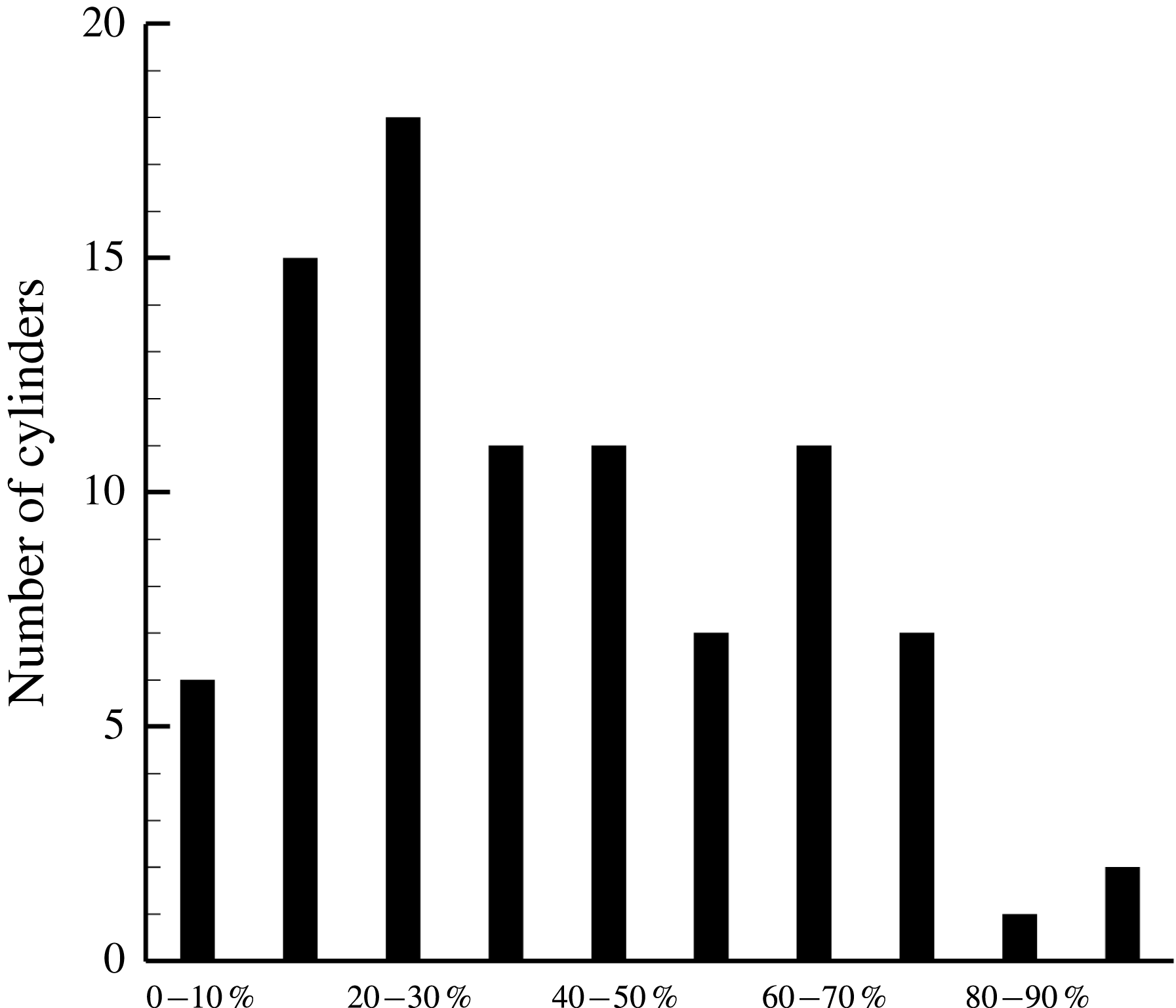
For cases with a large number of solid cylinders (e.g. the case
 $\text{SVF}=0.2$
for which
 $N=89$
), information on the distribution of the mean total force acting on the individual cylinders within the array is particularly relevant for applications related to flow past vegetated canopies. The histogram plot in figure 17 shows the number of cylinders in the array for which the magnitude of the mean total force acting on the individual cylinders is a certain fraction of the maximum mean total force among all cylinders in the array. Figures 16(a) and 17 show that the cylinders facing the flow are in different conditions from those in the middle part or rear of the array and that only a small fraction of the total number of cylinders is subject to forces that are comparable (e.g. within 20 %) to the maximum drag force. If the cylinders are organic (flexible plant stems), they may have different biological properties and oscillatory patterns, depending on their position in the array, and the statistics of such properties may correlate to the histogram.
Histogram showing the number of cylinders in the array for which the magnitude of the mean total force acting on the individual cylinders is a certain fraction of the maximum mean total force among all cylinders in the array. Ten bins were used when counting the number of cylinders in each interval based on the value of the mean total force. Results are shown for
 $\text{SVF}=0.2~(N=89)$
.

5.2. Non-dimensional forces acting on the porous cylinder
Using the time-averaged forces acting on the individual cylinders,
 $\overline{\boldsymbol{F}}^{n}=\overline{F}_{x}^{n}\boldsymbol{i}+\overline{F}_{y}^{n}\boldsymbol{j}$
, one can calculate the total mean force acting on the porous cylinder,
 $\overline{\boldsymbol{F}}=\sum _{n=1}^{N}\overline{\boldsymbol{F}}^{n}$
, and then define a total (streamwise) drag coefficient,
 $\overline{C}_{DG}=\overline{F}_{x}/(0.5{\it\rho}U^{2}D)$
, an average total drag coefficient normalized with the number of solid cylinders in the array,
 $\overline{C}_{D}=\overline{C}_{DG}/N$
, and an average solid cylinder drag coefficient,
 $\overline{C}_{d}=(\overline{C}_{DG}/N)(D/d)=(1/N)\sum _{n=1}^{N}\overline{C}_{D}^{n}$
. The strength of the temporal oscillations of the total drag and lift forces on the porous cylinder can be characterized by calculating the r.m.s. values of
 $C_{DG}=F_{x}/(0.5{\it\rho}U^{2}D)$
and
 $C_{LG}=F_{y}/(0.5{\it\rho}U^{2}D)$
, which are denoted
 $C_{DG,rms}$
and
 $C_{LG,rms}$
respectively.
Figure 18(a) compares the present predictions of
 $\overline{C}_{DG}$
with those of the 2D DNS of Nicolle & Eames (Reference Nicolle and Eames2011) obtained at a lower
 $\mathit{Re}_{D}$
and with the predictions of the analytical model proposed by the same authors. Overall, a good agreement is observed between the LES and DNS for cases with with
 $d/D=0.048$
, with 3D LES results being closer to the analytical model results. The results in figure 18(a) also show that the ratio
 $d/D$
has an important effect on
 $\overline{C}_{DG}$
. For
 $\text{SVF}=0.2$
, doubling of
 $d/D$
results in a 35 % decrease of
 $\overline{C}_{DG}$
. Another important observation is that for
 $\text{SVF}\geqslant 0.1$
,
 $\overline{C}_{DG}$
is larger than 1.17, which is the value for a solid cylinder of equal diameter (case
 $\text{SVF}=1$
). This is because for sufficiently large values of the SVF, the adverse pressure gradients acting on the porous cylinder (e.g. on the solid cylinders situated on or close to the upstream face of the porous region) become comparable to the ones induced on a solid cylinder of same diameter, but additionally there is drag acting on the interior cylinders because of the bleeding flow advected through the porous region. Following Nicolle & Eames (Reference Nicolle and Eames2011), we also plotted
 $\overline{C}_{D}$
as a function of the SVF in figure 18(b). The comparison is shown only for cases with
 $d/D=0.048$
. The analytical model predictions of
 $\overline{C}_{D}$
show good agreement with the numerical results, with 3D LES being slightly closer to the theoretical model for
 $\text{SVF}\approx 0.1$
.
Non-dimensional time-averaged streamwise drag force: (a) Time-averaged total drag coefficient for the array,
 $\overline{C}_{DG}$
versus SVF; (b) mean time-averaged total drag coefficient normalized by the number of solid cylinders in the array,
 $\overline{C}_{D}=\overline{C}_{DG}/N$
versus SVF; results are compared for constant
 $d/D$
; (c) mean time-averaged solid cylinder drag coefficient,
 $\overline{C}_{d}=(\overline{C}_{DG}/N)(D/d)$
versus SVF; (d) mean time-averaged solid cylinder drag coefficient,
 $\overline{C}_{d}$
, and combined drag parameter for the porous cylinder,
 $\overline{{\it\Gamma}}=\overline{C}_{d}(aD)/(1-\text{SVF})$
versus
 $aD$
. Filled circles and squares denote results of the present 3D LES. Hollow circles and squares denote results of the 2D DNS of Nicolle & Eames (Reference Nicolle and Eames2011). The solid black line corresponds to the analytical model of Nicolle & Eames (Reference Nicolle and Eames2011).

The most important parameter to be estimated from the present simulations is
 $\overline{C}_{d}$
. This is the main empirical constant that has to be provided in Reynolds-Averaged Navier–Stokes (RANS) and LES simulations that do not resolve the flow through the porous region and rather add a quadratic drag term in the momentum equations that is active over the porous region. This term is proportional to
 $\overline{C}_{d}$
and is generally assumed to be a constant for the quadratic drag regime (high Reynolds numbers) or, at best, a function of the SVF. The results in figure 18(c) show that
 $\overline{C}_{d}$
is a function of both the SVF and
 $d/D$
. For a constant
 $d/D$
ratio,
 $\overline{C}_{d}$
decreases in a nonlinear way with increase in the SVF. Finally, figure 18(d) shows that the non-dimensional frontal area,
 $aD$
, is a better variable to characterize the variation of
 $\overline{C}_{d}$
. This is because for cases with different values of the SVF and
 $d/D$
ratio,
 $\overline{C}_{d}$
decays monotonically with increase in
 $aD$
.
The results in figure 19 show that
 $C_{DG,rms}$
is mainly a function of the SVF, with
 $d/D$
having a minor influence. The peak value of
 $C_{DG,rms}$
is observed for
 $\text{SVF}=0.05$
, which corresponds to the threshold between the regime characterized by weak wake-to-cylinder interactions and a close-to-horizontal direction of the bleeding flow within the whole porous region and the regime where the von Karman vortex street is present and the bleeding flow has a strong lateral component. The variation of
 $C_{LG,rms}$
is qualitatively similar to that of
 $C_{DG,rms}$
, but the peak value occurs around
 $\text{SVF}=0.1$
. This is expected because of the strong amplification of the lift force fluctuations on solid cylinders situated within the upstream half of the porous region (figure 10
b). Although, on average, the lift force fluctuations are comparable or even slightly higher for
 $\text{SVF}=0.05$
(figure 10
c), the total number of solid cylinders within the same region is 50 % less compared with the case
 $\text{SVF}=0.1$
.
Effect of the volume fraction of solids and relative cylinder diameter,
 $d/D$
, on the r.m.s. of the total non-dimensional drag and lift forces acting on the solid cylinders within the array. Blue squares denote
 $C_{DG,rms}$
; red circles denote
 $C_{LG,rms}$
.

The resolved t.k.e. contour plots in figure 5(a) can also be used to identify the cases for which the largest r.m.s. values of the drag and lift forces acting on the porous cylinder are expected to occur. This is because the main contributor to the t.k.e. is the vortex shedding past the solid cylinders within the array (see supplementary movie_2). Consistent with results in figure 19, the simulations where the t.k.e. values within the porous region are the highest are those with
 $\text{SVF}=0.05$
and
 $\text{SVF}=0.1$
(figure 5
a).
The decay of
 $C_{LG,rms}$
with the volume fraction of solids observed for
 $\text{SVF}\geqslant 0.1$
in figure 19 is expected to last until the SVF is high enough such that the von Karman wake billows form at a small distance from the back of the porous region. Once that happens,
 $C_{LG,rms}$
should start increasing to approach the value (
 $C_{LG,rms}=0.63$
) predicted for a solid cylinder (case
 $\text{SVF}=1.0$
). The amplitude of the
 $C_{DG}$
oscillations is also expected to increase for very high values of the SVF. One should note that the value of
 $C_{DG,rms}$
corresponding to the solid cylinder case (
 $C_{DG,rms}=0.105$
for
 $\text{SVF}=1.0$
) is comparable to the relative peak observed for
 $\text{SVF}=0.05$
.
5.3. Combined drag parameter for the porous cylinder
For high-Reynolds-number cases, the viscous term is much smaller than the advective term in the dimensionless streamwise momentum equation. The dominant terms in the momentum balance within the porous region are the streamwise advection term
 $(1-\text{SVF})u(\partial u/\partial x)$
and the quadratic velocity drag term
 $\overline{C}_{d}au|u|$
, where
 $u$
is the local dimensionless streamwise velocity. The ratio between these two terms characterizes the relative influence of the drag term relative to the advection term. This ratio defines a combined drag parameter for the porous medium
 ${\it\Gamma}_{D}=\overline{C}_{d}\,aD/(1-\text{SVF})\cong \overline{C}_{d}(d/D)SVF/(1-\text{SVF})$
, where we assumed that
 $\partial u/\partial x$
is of the order of the mean deceleration of the streamwise velocity between the upstream and downstream ends of the porous patch. As both streamwise velocities are proportional to
 $U$
, and the average length of the porous patch is proportional to
 $D$
, the gradient is proportional to
 $U/D$
. Therefore, in the present case of a circular porous cylinder,
 ${\it\Gamma}_{D}$
is a measure of the relative deceleration of the streamwise velocity between the front and the back of the porous cylinder for a given total mean drag force. This parameter can also be thought of as a global measure of the obstacle density. The same parameter can be interpreted as the ratio of the porous cylinder diameter,
 $D$
, to the canopy drag length scale,
 $L_{c}=2(1-\text{SVF})/(\overline{C}_{d}a)$
, introduced by Belcher, Jerram & Hunt (Reference Belcher, Jerram and Hunt2003), if the multiplying constant in the definition of
 $L_{c}$
is ignored.
The range of
 ${\it\Gamma}_{D}$
in the present simulations was 0.68–2.57 (table 1). These values are within the range of values observed in vegetated channels (Jamali et al.
Reference Jamali, Zhang and Nepf2008). For relatively low values of the SVF,
 ${\it\Gamma}_{D}\cong \overline{C}_{d}\,aD$
. We have already shown that
 $\overline{C}_{d}$
varies monotonically with
 $aD$
for cases with different values of the SVF and
 $d/D$
. The results in figure 18(d) show that
 ${\it\Gamma}_{D}$
increases monotonically with
 $aD$
based on data from the present 3D LES and the 2D DNS of Nicolle & Eames (Reference Nicolle and Eames2011). Analysis of the
 $\text{SVF}=0.2(2\mathit{d})$
and
 $\text{SVF}=0.1$
simulations which are characterized by nearly equal values of
 ${\it\Gamma}_{D}$
showed that the reduction of the streamwise velocity across the porous cylinder,
 $U{-}U_{1}$
, is close in the two cases, which confirms the physical interpretation of
 ${\it\Gamma}_{D}$
.
Another important parameter is
 ${\it\Gamma}_{D}(d/D)=\overline{C}_{d}ad/(1-\text{SVF})$
(see table 1). This parameter characterizes the geometry of the porous medium within the circular patch. In the case of a layer of uniform SVF extending over the whole volume of the open channel, Tanino & Nepf (Reference Tanino and Nepf2008) have shown that
 ${\it\Gamma}_{D}(d/D)$
controls the turbulence intensity within the porous layer. This is not the case for the flow analysed here, where
 ${\it\Gamma}_{D}(d/D)$
peaks for
 $\text{SVF}=0.2(2\mathit{d})$
, while the maximum t.k.e. inside the porous region is observed for the cases
 $\text{SVF}=0.05$
and
 $\text{SVF}=0.1$
(figure 5
a). An important difference between the case of fully vegetated channels and the present set-up is that we consider long cylinders with no bottom surface. Therefore, there is no mean velocity gradient in the vertical direction.
In the context of fully vegetated channels, King, Tinoco & Cowen (Reference King, Tinoco and Cowen2012) found that
 ${\it\Gamma}_{D}(d/D)$
is a measure of scale separation between the dispersive kinetic energy due to production by mean vertical shear and the t.k.e. generated in the wakes of the solid cylinders mainly by large-scale unsteadiness (vortex shedding). In the flow set-up considered in the present study, the dispersive kinetic energy is mainly associated with production by mean horizontal shear (e.g. in regions where large mean velocity gradients are generated in between the solid cylinders) within the porous region. Indeed, the distributions of the time-averaged streamwise velocity,
 $\overline{u}/U$
, within the porous region in figure 20 confirm that the largest horizontal mean velocity gradients are observed in the case
 $\text{SVF}=0.2(2\mathit{d})$
, which is characterized by the largest value of
 ${\it\Gamma}_{D}(d/D)$
and a non-negligible contribution of the dispersive stress to the total (dispersive plus Reynolds) stress. The results for the time-averaged lateral velocity (not shown) are qualitatively similar. Finally, one should stress that
 ${\it\Gamma}_{D}$
and
 ${\it\Gamma}_{D}(d/D)$
are of equal significance for the case of a porous cylinder situated on a bottom boundary. One expects the values predicted for infinitely long cylinders to be very close to those estimated for patches of emerged cylinders, away from the bed region. Close to the bed, the values of the two variables will change because of the decay of the approaching velocity induced by the no-slip boundary. This will influence the cylinder Reynolds number and thus
 $\overline{C}_{d}$
.
Effect of the volume fraction of solids and relative cylinder size,
 $d/D$
, on the distribution of the mean flow streamwise velocity,
 $\overline{u}/U$
, within and downstream of the (porous) cylinder: (a)
 $\text{SVF}=0.2$
; (b)
 $\text{SVF}=0.2(2\mathit{d})$
; (c)
 $\text{SVF}=0.1$
.

6. Spatial extent of the wake region
The streamwise variations of the centreline profiles of the mean streamwise velocity,
 $\overline{u}/U$
, and the r.m.s. of the lateral velocity,
 $v_{rms}/U$
, are investigated in figure 21. Except for the
 $\text{SVF}=1.0$
case, the initial sharp variation (increase for low SVF cases and decrease for high SVF cases) of
 $\overline{u}/U$
at the back of the porous cylinder is followed by a region of mild decrease. Then,
 $\overline{u}/U$
starts to increase at a faster rate, as the streamwise velocity recovers towards
 $U$
. The velocity at the start of the region of mild decrease of
 $\overline{u}/U$
represents the velocity at the upstream end of the steady wake region and excludes the region that is strongly influenced by the wakes of the solid cylinders situated close to the back of the porous cylinder. This velocity is denoted
 $U_{1}/U$
in table 1. Some of the experiments of Zong & Nepf (Reference Zong and Nepf2012) found a close-to-constant value of
 $\overline{u}/U$
within the steady wake region. Rather than defining
 $U_{1}$
as the mean streamwise velocity along the steady wake region, we prefer to define
 $U_{1}$
as the velocity at the upstream end of the steady wake region. The two definitions are equivalent if
 $\overline{u}/U$
is close to constant.
Longitudinal profiles of the streamwise velocity,
 $\overline{u}/U$
(a), and the r.m.s. of the lateral velocity,
 $v_{rms}/U$
(b), measured along the centreline,
 $y/D=0$
. The vertical dashed lines mark the streamwise extent of the porous cylinder (
 $-0.5\leqslant x/D\leqslant 0.5$
). The black solid arrows in (a) show the end of the steady wake region based on the length
 $L_{1}$
. The black dash–dot–dot arrows in (a) show the end of the wake region based on the length
 $L$
. The dashed red arrows in (a) show the end of the wake region based on the length
 $L^{\prime }$
. The horizontal blue arrows in (a) denote the start of the steady wake region where
 $\overline{u}=U_{1}$
. The red solid arrows in (b) show the end of the steady wake region based on the length
 $L_{1}^{\prime \prime }$
. The red dashed arrows in (a) show the end of the wake region based on the length
 $L^{\prime \prime }$
.

The location of the minimum of
 $\overline{u}/U$
is a good indicator of the end of the steady wake region. The distance between this location and the back of the porous cylinder (
 $x/D=0.5$
) in denoted
 $L_{1}$
(table 1). The region of sharp increase of
 $\overline{u}/U$
is followed by a region where the rate of increase of
 $\overline{u}/U$
decreases strongly. Following Zong & Nepf (Reference Zong and Nepf2012), we define the total length of the wake region,
 $L$
(table 1), as the length from the back of the cylinder to the location where
 $\partial \overline{u}/U/\partial (x/D)$
becomes smaller than a threshold value. For cases where the von Karman vortex street forms, the distance
 $L$
approximately corresponds to the distance from the porous cylinder where the ends of the SSLs interact to form the wake billows. Figure 21 also contains another measure of the total length of the wake denoted
 $L^{\prime }$
(table 1), which extends until the end of the region of sharp increase of
 $\overline{u}/U$
. Obviously,
 $L^{\prime }$
is always smaller than
 $L$
.
Based on the centreline profiles of
 $v_{rms}/U$
in figure 21(b), two lengths are defined. The length
 $L^{\prime \prime }$
(table 1) is defined as the distance from the back of the porous cylinder to the location of the peak of
 $v_{rms}/U$
, which is denoted
 $v_{rms,max}/U$
in table 1. With the exception of the case
 $\text{SVF}=0.032$
for which no vortex street forms, all cases contain a well-defined peak of
 $v_{rms}/U$
. A region where
 $v_{rms}$
has a close-to-constant value is present starting at the back of the cylinder. This is followed by a region where
 $v_{rms}$
increases monotonically towards
 $v_{rms,max}$
. The distance from the back of the cylinder to the upstream end of the region, where
 $v_{rms}$
starts to increase monotonically, is denoted
 ${L_{1}}^{\prime \prime }$
(table 1). Analysis of the values of these lengths in table 1 shows that, to a very good approximation,
 $L^{\prime }=L^{\prime \prime }=L-1.5D$
and
 $L_{1}^{\prime \prime }<L_{1}$
. The advantage of using
 $L^{\prime \prime }$
rather than
 $L$
to define the length of the total wake region is that the position of
 $v_{rms,max}$
can be more easily and less ambiguously identified from measurements. In terms of the profile of
 $\overline{u}/U$
,
 $L^{\prime \prime }$
has a clear interpretation given that
 $L^{\prime \prime }=L^{\prime }$
. Probably, the use of
 $L_{1}^{\prime \prime }$
rather than
 $L_{1}$
to define the length of the steady wake region is a better option.
Following Zong & Nepf (Reference Zong and Nepf2012), figure 22(a,b) shows the variation of
 $L_{1}/D$
and
 $L/D$
with the ratio of the velocity at the start of the steady wake region to the maximum velocity in the acceleration region forming on the outer side of the SSLs,
 $U_{1}/U_{2}$
. Predictions of
 $L_{1}$
and
 $L$
by the present simulations follow the trend indicated by the experimental cases of Zong & Nepf (Reference Zong and Nepf2012). Consistent with experimental data, LES predicts a monotonic decay of
 $L_{2}/D$
with
 $v_{rms,max}/U$
(figure 22
c). Experiments and the present LES also predict a similar decay of
 $U_{1}/U$
with the SVF. Increasing
 $d/D$
, while keeping the SVF constant, results is a significant increase of
 $U_{1}/U$
.
Dependence of the main variables characterizing the near-wake region on the velocity ratio
 $U_{1}/U_{2}$
, the turbulence intensity
 $v_{rms,max}/U$
and the SVF: (a)
 $L_{1}/D$
versus
 $U_{1}/U_{2}$
; (b)
 $L/D$
versus
 $U_{1}/U_{2}$
; (c)
 $L_{2}/D$
versus
 $v_{rms,max}/U$
; (d)
 $U_{1}/U$
versus SVF. The experimental data of Zong & Nepf (Reference Zong and Nepf2012) are included. Here,
 $v_{rms,max}$
is the maximum value of the r.m.s. fluctuations of the lateral velocity along the centreline,
 $y/D=0$
, behind the porous cylinder.

Figure 23 presents a comparison between the present numerical predictions and laboratory experiments of Ball et al. (Reference Ball, Stansby and Allison1996), Takemura & Tanaka (Reference Takemura and Tanaka2007) and Chen et al. (Reference Chen, Ortiz, Zong and Nepf2012) for several main flow variables. Besides the steady wake velocity,
 $U_{1}$
, and the length of the steady wake region,
 $L_{1}$
, the third variable represented in figure 23 is the exit velocity,
 $U_{e}$
, which is the mean streamwise velocity along the centreline (
 $y/D=0$
) right at the back of the porous cylinder (
 $x/D=0.52$
). Following Chen et al. (Reference Chen, Ortiz, Zong and Nepf2012), these variables are plotted as a function of a non-dimensional flow blockage parameter,
 $C_{d}^{\prime }aD$
, which is the ratio of the porous cylinder diameter,
 $D$
, and a drag length scale
 $(C_{d}^{\prime }a)^{-1}$
. To allow a direct comparison with the experimental data, the drag coefficient,
 $C_{d}^{\prime }$
, is estimated based on the value of the Reynolds number defined with the cylinder diameter and the mean flow velocity within the porous cylinder region using the procedure presented by Tanino & Nepf (Reference Tanino and Nepf2008). As seen from the plots in figure 23, the numerical simulations not only capture the general trend in the variation of these three variables with
 $C_{d}^{\prime }\,aD$
, but also predict values that are, in most cases, within the scatter shown by the experimental data.
Dependence of the main variables characterizing the near-wake region on the non-dimensional flow blockage parameter,
 $C_{d}^{\prime }\,aD$
: (a) steady wake velocity,
 $U_{1}/U$
; (b) length of the steady wake region,
 $L_{1}/D$
; (c) exit velocity,
 $U_{e}/U$
. Data from several experimental studies (black hollow symbols) are included together with 3D LES predictions (red filled symbols).

7. Summary and conclusions
In this paper, 3D LES was used to understand how the volume fraction of solids (SVF) and the relative diameter of the cylinders in the array,
 $d/D$
, affect the flow and turbulence structure inside and downstream of an isolated circular array of solid cylinders at a porous cylinder Reynolds number (
 $\mathit{Re}_{D}=10\,000$
) that is high enough that energetic three-dimensional eddies are generated via vortex stretching. Simulations showed that for
 $\text{SVF}>0.1$
the flow becomes highly three-dimensional over most of the array (porous) region, while for
 $\text{SVF}<0.025$
3D effects are relatively small inside the porous region and the flow becomes highly 3D only downstream of the porous cylinder. Compared with the limiting case of a solid cylinder (
 $\text{SVF}=1.0$
), the presence of the bleeding flow through the porous region impedes the formation of wake billows at the back of the porous cylinder and pushes the main separation bubble away from the porous cylinder. The wake billows shed from the cylinders situated close to the lateral extremities of the porous region are an important source of large-scale turbulence for the SSLs of the porous cylinder. This is why the SSLs are much more energetic for a porous cylinder of sufficiently high SVF compared with a solid cylinder.
Two distinct flow regimes were identified. The first one is observed for sufficiently high values of the SVF for which wake billows with alternate directions of rotations are shed in the wake of the porous cylinder, similar to the von Karman vortex street regime observed for solid cylinders at sufficiently high
 $\mathit{Re}_{D}$
. The second one is observed for sufficiently low values of the SVF where no von Karman vortex street forms behind the porous cylinder and the wake-to-cylinder interactions within the array are relatively weak. The threshold value of the SVF that determines which regime occurs is in between 0.1 and 0.05. A first important finding of this study is that well-defined SSLs form on the sides of the porous cylinder even in the second regime (e.g. for
 $\text{SVF}=0.023$
), and that these SSLs are subject to in-phase large-scale undulatory motions with a frequency that is close to that corresponding to the shedding of wake billows in the first regime (
 $\mathit{St}_{D}\approx 0.2{-}0.24$
). This result is consistent with experimental measurements of velocity spectra in the wake of porous cylinders. Although this non-dimensional frequency was also observed in the experiments of Zong & Nepf (Reference Zong and Nepf2012) conducted with low values of the SVF, no explanation was provided for the mechanism responsible for its presence. A second important finding is that no intermediate regime in which the force acting on the solid cylinders is close to steady is observed. Such a regime was observed in the 2D DNS study of Nicolle & Eames (Reference Nicolle and Eames2011). To confirm that this is not an artefact due to the different numerical approach used in the two studies, we ran 2D LES for some of the cases discussed in the present paper. The 2D LES results were found to be fully consistent with the findings of Nicolle & Eames (Reference Nicolle and Eames2011). This shows the importance of using a fully 3D model to study the physics of these flows. Moreover, the fine-resolution data from the numerical simulations allowed us to propose less ambiguous ways to define the lengths of the steady wake and total wake regions, which are two important length scales used to analyse these flows (Chen et al.
Reference Chen, Ortiz, Zong and Nepf2012; Zong & Nepf Reference Zong and Nepf2012).
A main advantage of the present numerical approach, in which the flow around the cylinders in the array is resolved, is that the drag and lift forces on the individual cylinders can be evaluated as functions of the non-dimensional parameters describing the array of cylinders. The results showed that depending on the SVF and
 $d/D$
, some of the cylinders within the array can be subject to highly unsteady drag and lift forces whose mean amplitudes can be much larger than the values observed for an isolated cylinder. Except for cases with a very low SVF, the maximum drag forces on the individual cylinders within the array occur on the interior cylinders rather than on the ones directly exposed to the incoming flow. The relationships showing the variation of the r.m.s. values of the drag and lift forces acting on the cylinders as a function of the SVF provide additional valuable information to characterize the unsteadiness of the drag forces. These findings have important consequences especially for vegetated flows where the plant stems are flexible.
Using the approach advocated in the present paper, the mean time-averaged drag coefficient for the cylinders in the array,
 $\overline{C}_{d}$
, can be directly estimated. This is important given the scarcity of detailed experimental data on drag coefficients for arrays of cylinders and, in particular, for finite arrays. Moreover,
 $\overline{C}_{d}$
is the main parameter that has to be provided to simpler, computationally much less expensive, numerical models not resolving the flow around individual cylinders. The present results show that
 $\overline{C}_{d}$
is mainly a function of the non-dimensional frontal area,
 $aD$
.
The combined drag parameter for the porous cylinder,
 ${\it\Gamma}_{D}=\overline{C}_{d}\,aD/(1-\text{SVF})$
, is the key grouping of parameters that determines by how much the velocity of the bleeding flow at the back of the porous cylinder is reduced compared with the incoming flow velocity for a given total drag force acting on the porous cylinder. Results from simulations conducted with different SVF,
 $d/D$
and
 $\overline{C}_{d}$
show that
 ${\it\Gamma}_{D}$
increases monotonically with increasing
 $aD$
.
The present work considered only the case of an incoming steady flow (no resolved turbulence). A future direction of study will be to investigate how the level of turbulence in the incoming flow modifies the mean flow and turbulence statistics within and downstream of the porous cylinder and how it affects the forces acting on the cylinders within the array. The present work, focusing on an isolated circular patch containing long solid cylinders, can be considered as a limiting case for two other important categories of applications, which are of particular relevance for flow in vegetated channels. The first category of applications concerns porous patches placed in a channel with a bottom wall. The second category of applications concerns flow past arrays of porous cylinders (e.g. vegetation mosaics), where wake-to-porous-cylinder interactions are significant. Such applications will be considered in future work.
Acknowledgements
We gratefully acknowledge the National Center for High Performance Computing (NCHC) in Taiwan and the Transportation Research and Analysis Computing Center (TRACC) at the Argonne National Laboratory for providing substantial computer time.
Supplementary movies
Supplementary movies are available at http://dx.doi.org/10.1017/jfm.2015.321.