


1. Introduction
Low Reynolds number ( $Re$) viscoelastic flow of polymeric fluids is inherent in a wide range of problems of scientific and industrial interest, including secondary flows in DNA and blood suspensions and a variety of polymeric products (Benzi & Ching Reference Benzi and Ching2018). The intricate flow microstructure coupling in complex fluids gives rise to a host of flow instabilities that are unique to viscoelastic fluids (Shaqfeh & Khomami Reference Shaqfeh and Khomami2021). Chief among these is the fascinating flow state dubbed ‘elastic turbulence’ (ET) that occurs solely due to the highly nonlinear dynamics of the elastic stresses at very small
 $Re$ (
 $\ll 1$) and sufficiently large Weissenberg number,
 $Wi\gg 1$ (Groisman & Steinberg Reference Groisman and Steinberg2000). The existence of this inertialess turbulent flow was experimentally discovered by Steinberg and co-workers in a host of curvilinear shear flows of dilute polymeric solutions where hoop stresses are the main driving force for the onset of a purely elastic instability and subsequent flow transitions that lead to the ET flow state (Groisman & Steinberg Reference Groisman and Steinberg2004). Unlike the inertially driven high-
 $Re$ turbulence that has been studied for centuries, this low-
 $Re$ turbulent flow with widespread applications in many important physio-chemical processes is far less understood, particularly from a mechanistic standpoint.
Purely elastic instabilities at  $Re\ll 1$ have been observed in a large variety of curvilinear flow geometries, cone-and-plate and parallel plate torsional flows, cross-channel flows as well as flows past obstacles (Larson, Shaqfeh & Muller Reference Larson, Shaqfeh and Muller1990; Shaqfeh Reference Shaqfeh1996; Khomami & Moreno Reference Khomami and Moreno1997; De et al. Reference De, van der Schaaf, Deen, Kuipers, Peters and Padding2017). To date, the most comprehensive studies of purely elastic instability and higher-order flow transitions have been performed on the Taylor–Couette (TC) flow, namely, the flow between two independently rotating coaxial cylinders (Taylor Reference Taylor1923; Larson et al. Reference Larson, Shaqfeh and Muller1990; Shaqfeh, Muller & Larson Reference Shaqfeh, Muller and Larson1992). In addition, the non-axisymmetric linear (Avgousti & Beris Reference Avgousti and Beris1993) and weakly nonlinear (Sureshkumar, Beris & Avgousti Reference Sureshkumar, Beris and Avgousti1994; Renardy et al. Reference Renardy, Renardy, Sureshkumar and Beris1996) stability analyses of viscoelastic TC flow have demonstrated that the most unstable mode of the inertia-free instability is indeed three-dimensional (3-D) and time dependent. Specifically, non-axisymmetric flow patterns after the onset of the purely elastic instability, namely, ribbons (standing waves) and spirals (travelling waves) are observed (Avgousti & Beris Reference Avgousti and Beris1993). Moreover, Sureshkumar et al. (Reference Sureshkumar, Beris and Avgousti1994) have shown that, for a narrow gap geometry, at least one of the non-axisymmetric flow patterns bifurcates subcritically; while in the wide gap geometry both bifurcations are supercritical. These comprehensive experimental and theoretical studies have clearly demonstrated that this inertialess instability occurs due to the coupling of the radial velocity gradient perturbations and azimuthal shear induced hoop stresses. Higher-order flow transitions show very rich and often highly localized flow patterns, such as rotating standing waves, disordered oscillations, oscillatory strips and solitary vortex pairs or ‘diwhirls’ (Groisman & Steinberg Reference Groisman and Steinberg1997; Dutcher & Muller Reference Dutcher and Muller2009). To that end, large-scale diwhirls that arise due to the symmetry breaking of inflow/outflow patterns have been shown to be a fundamental building block of the spatio-temporal dynamics of higher-order flow transitions in the viscoelastic TC flow of the highly elastic regime (Groisman & Steinberg Reference Groisman and Steinberg1997, Reference Groisman and Steinberg2004). In fact, the presence of the aforesaid asymmetry in the measured radial velocity distribution is a hallmark of ET in TC flow (Groisman & Steinberg Reference Groisman and Steinberg2004).
Extensive experimental and theoretical studies have shown that ET is essentially a spatially smooth and temporally random flow that exhibits a broad range of spatio-temporal scales with a steep power law decay in the velocity power spectra at nearly all scales (Fouxon & Lebedev Reference Fouxon and Lebedev2003; Steinberg Reference Steinberg2019). Moreover, the stress analogy between ET and magnetohydrodynamics suggests that elastic waves with a  $Wi$ dependent speed in ET are similar to Alfvén waves (Varshney & Steinberg Reference Varshney and Steinberg2019). However, the lack of experimental techniques for in situ measurement of elastic stresses strongly limits the much-needed mechanistic understanding of the turbulent dynamics in ET. To that end, recent direct numerical simulations (DNS) of two-dimensional (2-D) ET in Kolmogorov (Berti et al. Reference Berti, Bistagnino, Boffetta, Celani and Musacchio2008; Berti & Boffetta Reference Berti and Boffetta2010; Garg, Calzavarini & Berti Reference Garg, Calzavarini and Berti2021) and TC flows (Buel, Schaaf & Stark Reference Buel, Schaaf and Stark2018) have shown reasonable agreements with the statistics and steep energy spectra decay of the experimentally measured velocities. Specifically, in the Kolmogorov flow, essentially identical scaling in both temporal and spatial spectra of velocity fluctuations has been reported, namely, an exponent of approximately
 $-4$ (Garg et al. Reference Garg, Calzavarini and Berti2021). In addition, Buel et al. (Reference Buel, Schaaf and Stark2018) have clearly shown that scaling exponents in temporal and spatial frequency domains exhibit strong variations in the radial direction in TC flow. These discrepancies raise serious concern about the validity of Taylor's frozen-field hypothesis that is used in experimental investigation of the ET flow state (Garg et al. Reference Garg, Calzavarini and Berti2021). Since both the theory and experiments deal with 3-D flows, the 2-D DNS results cannot accurately capture the essential flow–microstructure coupling of the turbulent dynamics in the ET flow state. Hence, the 3-D simulations are required to pave the way for a full mechanistic understanding of ET in prototypical curvilinear flows.
Due to the well-known ‘high  $Wi$ problem’, 3-D DNS of purely elastic flow (
 $Re\ll 1$) has remained a grand challenge problem for the computational non-Newtonian fluid mechanics community (Talwar, Ganpule & Khomami Reference Talwar, Ganpule and Khomami1994; Yang & Khomami Reference Yang and Khomami1999; Alves, Oliveira & Pinho Reference Alves, Oliveira and Pinho2021). To that end, the results of the first 3-D DNS of ET in TC flows of dilute polymeric solutions are presented. Specifically, it is shown that, at a fixed
 $Wi=30$, reducing
 $Re$ from
 $1000$ to
 $0.0001$ leads to an intriguing transition route from an elastically dominated turbulent (EDT) flow state to a diwhirls dominated flow state and finally to ET. The simulation results demonstrate a significant enhancement of flow resistance and a steep power law decay in velocity power spectra in accord with the seminal experimental work of Groisman & Steinberg (Reference Groisman and Steinberg2004). Finally, the spatio-temporal characteristics of ET and the different mechanisms that give rise to turbulent fluctuations in the EDT and ET flow states are discussed in detail.
2. Numerical details
Three-dimensional DNS has been performed by a recently developed hybrid spectral/finite-difference parallel algorithm (Song et al. Reference Song, Lin, Liu, Lu and Khomami2021a). We have chosen  $d=R_o-R_i$,
 $d/(\varOmega R_i)$,
 $\varOmega R_i$,
 $\rho (\varOmega R_i)^{2}$ and
 $\eta _p \varOmega R_i / d$ as scales for length, time, velocity
 $\boldsymbol {u}$, pressure
 $P$, and polymer stress
 $\boldsymbol {\tau }$, respectively. Here,
 $R_i$ and
 $R_o$ are the inner and outer cylinder radii, respectively;
 $\varOmega$ denotes the inner cylinder angular velocity, and
 $\rho$ the solution density. The polymer stress
 $\boldsymbol {\tau }$ is related to the conformation tensor
 $\boldsymbol{\mathsf{C}}$ through the FENE-P (finitely extensible nonlinear elastic-Peterlin) model (Bird et al. Reference Bird, Curtiss, Armstrong and Hassager1987). The dimensionless governing equations for the incompressible flow of a FENE-P fluid are
 \begin{gather} \boldsymbol{\nabla}\boldsymbol{{\,\cdot\,}}\boldsymbol{u} = 0, \end{gather}
 \begin{gather} \frac{\partial \boldsymbol{u}}{\partial t}+\boldsymbol{u}\boldsymbol{{\,\cdot\,}}\boldsymbol{\nabla}\boldsymbol{u} ={-}\boldsymbol{\nabla} P+\frac{\beta}{Re}\nabla^{2}\boldsymbol{u}+\frac{1-\beta}{Re}\boldsymbol{\nabla}\boldsymbol{{\,\cdot\,}}\boldsymbol{\tau}, \end{gather}
and
 \begin{equation} \frac{\partial \boldsymbol{\mathsf{C}}}{\partial t} + \boldsymbol{u}\boldsymbol{{\,\cdot\,}}\boldsymbol{\nabla}\boldsymbol{\mathsf{C}}=\boldsymbol{\mathsf{C}}\boldsymbol{{\,\cdot\,}}\boldsymbol{\nabla}\boldsymbol{u} +(\boldsymbol{\nabla}\boldsymbol{u})^{\rm T}\boldsymbol{{\,\cdot\,}}\boldsymbol{\mathsf{C}}-\boldsymbol{\tau}, \end{equation}
where polymer molecules are modelled as dumbbells composed of two beads and a nonlinear spring. The polymeric stress  $\boldsymbol {\tau }$ is related to the polymer conformation tensor
 $\boldsymbol{\mathsf{C}}$ via the relationship
 $\boldsymbol {\tau }=(\,f(\boldsymbol{\mathsf{C}})\boldsymbol{\mathsf{C}}-\boldsymbol{\mathsf{I}})/Wi$, where
 $f(\boldsymbol{\mathsf{C}})=(L^{2}-3)/(L^{2}-{{\rm trace}}(\boldsymbol{\mathsf{C}}))$ is the Peterlin function and
 $L$ represents the maximum chain length. The Reynolds number is defined as
 $Re=\rho \varOmega R_i d/\eta _t$, where
 $\eta _t$ represents the sum of the solvent (
 $\eta _s$) and polymer (
 $\eta _p$) viscosities and
 $\beta =\eta _s / \eta _t$. The Weissenberg number is defined as
 $Wi=\lambda \varOmega R_i /d$, with
 $\lambda$ being the polymer relaxation time. The governing equations are supplemented with no-slip boundary conditions at walls, as well as periodic boundary conditions in the axial direction with a periodicity length of
 ${\rm \pi} d$. This hybrid algorithm is numerically stable and preserves the positive definiteness as well as the boundedness of the polymer conformation tensor (
 $0<{{\rm trace}}(\boldsymbol{\mathsf{C}})< L^{2}$) without the addition of a global artificial diffusion term to the conformation tensor evolution equation (Song et al. Reference Song, Lin, Liu, Lu and Khomami2021a).
Our recent studies of EDT in TC flows suggest that the ET flow state should be realized in a large curvature TC system, i.e.  $\eta =R_i /R_o=0.5$, filled with a dilute polymer solution with
 $\beta =0.9$ and
 $L=100$ by increasing the elasticity number (
 $El=Wi/Re$) via decreasing
 $Re$ from
 $1000$ to
 $0.0001$ at
 $Wi=30$. Specifically, as
 $Re$ is progressively decreased, the converged numerical results at a higher
 $Re$ are used as the initial flow field. Guided by our previous calculations (Liu & Khomami Reference Liu and Khomami2013; Song et al. Reference Song, Lin, Liu, Lu and Khomami2021a), a large mesh size of
 $128\times 128\times 256$ for the
 $r\times \theta \times z$ directions and an extremely small time step of
 $0.00025$ is used to reliably capture the velocity and polymer stress fields at related scales (see grid validation in the Appendix). Sufficiently long simulations (typically of
 $\sim 20\lambda$) are performed to ensure that the statistically stationary flow states have been realized. Moreover, ensemble averages are obtained over a time period of
 $\sim 10\lambda$.
3. Results and discussion
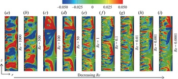
As depicted by figure 1, progressive increase of  $El$ via decreasing
 $Re$ leads to a clear flow transition sequence, namely, from a flow state with irregular large-scale streamwise vortices commonly observed in the EDT flow regime to a flow field with well organized and nearly spatially localized vortices at
 $Re=100$ and
 $Re=50$ (figure 1c,d). The appearance of solitary vortex pairs or diwhirls has been extensively documented in experimental studies of elastically dominated viscoelastic TC flow and it is widely regarded as a signature of the flow state that leads to ET (Groisman & Steinberg Reference Groisman and Steinberg1997; Dutcher & Muller Reference Dutcher and Muller2009). Hence, it is not surprising that further decrease of
 $Re$ leads to another flow transition to a chaotic flow state, particularly near the inner wall. The ET flow state is reached at
 $Re=1$ (see figure 1e–i). The vortical structures seen in this chaotic flow show very little change with further decrease of
 $Re$ from
 $Re=1$ to
 $Re=0.0001$. The fact that the dominant flow structures are insensitive to a four orders of magnitude reduction of
 $Re$ is a clear indication that this chaotic turbulent state can be considered inertia free. Hence, it indeed corresponds to a purely elastic turbulent state, namely, ET. The dominant flow structures in the ET consist of two pairs of diwhirls that nearly span the entire gap along with numerous small-scale streamwise vortices randomly distributed near the inner wall. As demonstrated in our previous studies, these small-scale streamwise vortices are elastic Görtler vortices (Song et al. Reference Song, Teng, Liu, Ding, Lu and Khomami2019). Surprisingly, these vortices wrap up in the left half-side of the diwhirls. This is reminiscent of the inertial Görtler vortices formed over the convex inner wall that are nested to large-scale Taylor vortices in high-
 $Re$ TC turbulence (Wei et al. Reference Wei, Kline, Lee and Woodruff1992). However, it is evident that these two sets of nested flow structures have a totally different driving mechanism as diwhirls and elastic Görtler vortices are formed as a consequence of elastically driven flow transitions.
Time and  $\theta$-direction averaged vectors of radial (
 $\langle u_r\rangle _{\theta, t}$) and axial (
 $\langle u_z\rangle _{\theta, t}$) velocities and contour plots of streamwise vorticity
 $\langle \omega _\theta \rangle _{\theta, t}$ in an (
 $r, z$) plane for various
 $Re$ with
 $Wi=30$,
 $0\leq z \leq {\rm \pi}d$ and
 $R_i\leq r\leq R_o$.

As  $Re$ decreases, the Nusselt number (
 $Nu_\omega = J^{\omega }/J^{\omega }_{lam}$, where
 $J^{\omega }$ is the angular momentum current and
 $J^{\omega }_{lam}$ is its Newtonian laminar flow counterpart) of both viscoelastic and Newtonian TC flows decreases monotonically, as depicted in table 1. It should be noted that, when
 $Re \leq 1$, the Newtonian flows are laminar, i.e. azimuthal Couette flows with the angular momentum
 $ru_\theta$ transported solely by molecule diffusion, and
 $J^{\omega }=J^{\omega }_{lam}=2\varOmega R_i^{2} R_o^{2} /Re(R_i^{2}-R_o^{2})$. In the EDT flow state, i.e.
 $Re \ge 1$ DE first decreases due to a flow transition to a diwhirls dominated flow state. In turn, DE increases to its maximum of
 $103\,\%$ as a result of the stronger flux caused by the coherent large-scale vortical structures; subsequently, it decreases to
 $100\,\%$ once ET begins to set in at
 $Re=1$. Afterwards, the DE in ET state decreases slightly with further decrease in
 $Re$. This could be attributed to slight increase in the ratio of viscous forces to the stochastic polymeric body forces as
 $Re$ becomes vanishingly small. Specifically, for the viscoelastic TC flow,
 $J^{\omega }$ is written as
 \begin{equation} J^{\omega}=r^{3}(\langle u_r\omega \rangle- \nu_s \partial_r \langle\omega\rangle - \nu_p\langle\tau_{r\theta}\rangle/r). \end{equation}
Where  $\nu _s=\beta /Re$ and
 $\nu _p=(1-\beta )/Re$ are the dimensionless kinematic viscosities for solvent and polymers, respectively. The angular velocity
 $\omega = u_\theta /r$. The right-hand side terms of (3.1) represent in sequence the contribution of the convective flux (
 $J^{\omega }_c$), the diffusive flux (
 $J^{\omega }_d$) and the elastic source/sink term (
 $J^{\omega }_p$) to angular momentum (Song et al. Reference Song, Teng, Liu, Ding, Lu and Khomami2019). Also,
 $\langle \,\rangle =\langle \langle \langle \, \rangle _\theta \rangle _z\rangle _t$, denotes hereafter averaging in the
 $\theta$-direction,
 $z$-direction and time and the fluctuating part of variable
 $v$ is obtained as
 $v'=v-\langle v\rangle$. For a statistically stationary turbulent TC flow,
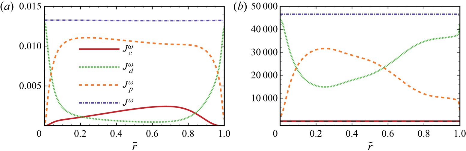
 $J^{\omega }$ should be constant across the gap (Eckhardt, Grossmann & Lohse Reference Eckhardt, Grossmann and Lohse2007). In the EDT flow state (see figure 2a), the elastic contribution
 $J^{\omega }_p$ is much larger than the small but non-zero inertial term
 $J^{\omega }_c$ in transporting angular momentum current in the bulk flow regime. However, in the ET flow state, the dominant contribution to
 $J^{\omega }$ comes from
 $J^{\omega }_p$ in the bulk and diffusive flux in the wall regions, while the inertial convection flux, as expected, is zero (figure 2b). This result fully supports the hypothesis proposed by Groisman & Steinberg (Reference Groisman and Steinberg2000) that the increase in the flow resistance in the ET flow state is solely due to elastic stresses.
Balance of angular momentum current across the gap for viscoelastic TC flows of (a) EDT with  $Re=1000$ and (b) ET with
 $Re=0.0001$. Hereafter,
 $\tilde {r}=(r-R_i)/d$ is the dimensionless distance to the inner cylinder wall. Here,
 $J^{\omega }_c$ represents the convective flux,
 $J^{\omega }_d$ is the diffusive flux and
 $J^{\omega }_p$ is the elastic source/sink term to total angular momentum current
 $J^{\omega }$.

Nusselt number and drag enhancement (DE) for various  $Re$. Here,
 $Nu_\omega ^{V}$ and
 $Nu_\omega ^{N}$ are the Nusselt number of viscoelastic and Newtonian TC flows, respectively and DE is calculated as
 $(Nu_{\omega }^{V}-Nu_{\omega }^{N})/Nu_{\omega }^{N}$.

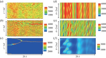
The spatio-temporal characteristics of the polymer chain extension ( ${\rm trace}(\boldsymbol{\mathsf{C}}$)) that results in significant elastic stresses are shown in figure 3. Similar to the 2-D simulation results of Buel et al. (Reference Buel, Schaaf and Stark2018), a strong radial dependence is observed. Specifically, near the inner wall (see figure 3a) travelling wave-like and local rotating standing waves are seen. The rotating standing waves appear as ribbons which can be viewed as a superposition of two counter-propagating upward and downward spiral waves of the same amplitude (Groisman & Steinberg Reference Groisman and Steinberg1996; Thomas, Khomami & Sureshkumar Reference Thomas, Khomami and Sureshkumar2006). However, in the ET flow state, the upward and downward spiral waves have slightly different amplitudes thus the flow patterns are also reminiscent of the disordered oscillations observed in experiments (Groisman & Steinberg Reference Groisman and Steinberg1996). The disordered oscillations are non-axisymmetric as evidenced by the travelling wave-like patterns in the azimuthal space–time plot (see figure 3d,e). At the middle gap (see figure 3b), the axially and azimuthally travelling wave-like flow patterns are not easily discerned and the spatio-temporal flow characteristic is essentially chaotic. However, near the outer wall, as seen in figure 3(c), the flow has a much simpler structure, namely, it is composed of only two localized intensive inflows associated with the diwhirls which eventually coalesce to form one diwhirl. In the azimuthal direction (see figure 3f), the travelling wave-like patterns are not easily discerned. As demonstrated by the non-axisymmetric nonlinear stability analysis of viscoelastic TC flow in the purely elastic regime, for the wide gap system, the possible flow patterns, i.e. ribbons (standing waves) and spirals (travelling waves) bifurcated supercritically (Sureshkumar et al. Reference Sureshkumar, Beris and Avgousti1994). Hence, these two flow patterns are stable after the purely elastic instability sets in even at higher perturbation amplitudes (fully nonlinear regime). In the present purely ET flow of
 $\eta =0.5$, both non-axisymmetric and time-dependent ribbons and travelling wave flow patterns are observed, clearly supporting the weekly nonlinear analysis results of Sureshkumar et al. (Reference Sureshkumar, Beris and Avgousti1994). Moreover, the large-scale diwhirls are shown to span across the gap and mainly dominate the outer gap region. The existence of the large-scale 3-D vortex structure and its extensional nature elucidated in previous TC flow experiments has been considered as a precursor to the ET (Groisman & Steinberg Reference Groisman and Steinberg2004). Overall, the spatio-temporal characteristics of polymer chain extension quantified via
 ${\rm trace}(\boldsymbol{\mathsf{C}})$ indicate the polymer chains are highly stretched in the two localized positions of diwhirls near the outer wall and the inner half-gap regions. With the exception in these two regions, the polymer chains exhibit significant temporal and spatial oscillations i.e. a stochastic stretch/relaxation behaviour. The rapid stochastic-like cycles of the polymer stretch and relaxation events give rise to significant fluctuations in elastic stresses/body forces over a broad frequency range. Hence, the flow–microstructure coupling will give rise to a strong feedback to the flow dynamics.
Axial and azimuthal space–time plots of polymer chain extension  ${{\rm trace}}(\boldsymbol{\mathsf{C}})$ obtained along a line near the inner wall (
 $\tilde {r}=0.01$): (a,d); at the middle gap (
 $\tilde {r}=0.5$): (b,e) and near the outer wall (
 $\tilde {r}=0.99$): (c,f), respectively, for ET at
 $Re=0.0001$,
 $Wi=30$.

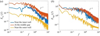
The aforementioned complex spatio-temporal dynamics of the flow can be quantified via examination of the temporal power spectral density of the radial fluctuating velocity and elastic normal stresses. As expected (see figure 4), both quantities display a steep power law decay in the frequency domain, especially at the inner half-gap, where the flow exhibits significant elastic turbulent characteristics. Moreover, the power law decay exponents seen in figure 4 are consistent with the theoretical study of Fouxon & Lebedev (Reference Fouxon and Lebedev2003), where it is shown that, in the ET flow state, the energy spectrum has to decay faster than  $f^{-3}$, where
 $\,f$ is the time frequency. Specifically, for the velocity spectra shown in figure 4(a), a continuous power law decay behaviour with an exponent of approximately
 $f^{-7}$ is observed over a decade at high frequencies. For the elastic stress spectra (see figure 4b), a steep power law decay with an exponent of approximately
 $f^{-5}$ at the middle gap and near the inner wall is observed. It should also be noted that the theoretical analysis of scaling relations in ET performed by Steinberg (Reference Steinberg2019) shows that the algebraic decay exponent of the elastic stress power spectrum
 $\nu$ should be
 $\alpha -2$, where
 $\alpha$ is power law exponent of the velocity energy spectra in a frequency domain. Our results of
 $\alpha =7$ and
 $\nu =5$ clearly support the result of this analysis. Despite the many successes of our 3-D DNS simulations in capturing flow features in the ET flow regime, the mechanism by which the fluctuating velocities in ET are produced is still far from fully understood.
The temporal power spectral density  $E_{u_r}(\,f)$ of (a) radial velocity
 $u_r$, and
 $E_{\tau _{\theta \theta }}(\,f)$ of (b) elastic normal stress
 $\tau _{\theta \theta }$ of ET at different radial locations with
 $Re=0.0001$,
 $Wi=30$.

The absence of Reynolds shear stress ( $J^{\omega }_c=r^{2}\langle u_r u_\theta \rangle =r^{2}\langle u'_r u'_\theta \rangle$, see figure 2b) in ET indicates that the turbulent kinetic energy (TKE,
 $E_t=\langle \boldsymbol {u}^{\prime } \boldsymbol {{\,\cdot\, }} \boldsymbol {u}^{\prime }\rangle /2$) cannot be generated by the typical shear production term (
 $\partial _r \langle u_\theta \rangle \langle u'_r u'_\theta \rangle$) in classical Newtonian turbulence. Hence, it has to be solely generated by the transformation of stored elastic potential energy (EPE,
 $E_p=\nu _p(L^{2}-3)\langle \ln (\,f(\boldsymbol{\mathsf{C}}))\rangle /2Wi$) in stretched polymers. For viscoelastic turbulent flow, the budget equation of
 $E_t$ is given as
 \begin{align} \frac{\partial E_t}{\partial t}+\boldsymbol{U}\boldsymbol{{\,\cdot\,}}\boldsymbol{\nabla} E_t & = \boldsymbol{\nabla}\boldsymbol{{\,\cdot\,}}( \underbrace{-\langle P^{\prime} \boldsymbol{u}^{\prime}\rangle}_{D_{p}}+\underbrace{2\nu_s\langle\boldsymbol{u}^{\prime} \boldsymbol{{\,\cdot\,}}\boldsymbol{\mathsf{s}}^{\prime}\rangle}_{D_{s}}+\underbrace{\nu_p\langle\boldsymbol{u}^{\prime} \boldsymbol{{\,\cdot\,}}\boldsymbol{\tau}^{\prime}\rangle}_{D_{e}}\underbrace{-\langle\boldsymbol{u}^{\prime} \boldsymbol{u}^{\prime}\boldsymbol{{\,\cdot\,}}\boldsymbol{u}^{\prime}\rangle/2}_{D_{t}} ) \nonumber\\ &\quad \underbrace{-2\nu_s\langle\boldsymbol{\mathsf{s}}^{\prime}:\boldsymbol{\mathsf{s}}^{\prime}\rangle}_{\varepsilon} \underbrace{-\nu_p\langle\boldsymbol{\mathsf{s}}^{\prime}:\boldsymbol{\tau}^{\prime}\rangle}_{P_{e}} \underbrace{-\langle\boldsymbol{u}^{\prime}\boldsymbol{u}^{\prime}\rangle:(\boldsymbol{\nabla}\boldsymbol{U})}_{P_{t}}, \end{align}
and the budget equation for polymer additive EPE  $E_p$ (Dallas & Vassilicos Reference Dallas and Vassilicos2010) is
 \begin{align} \frac{\partial E_p}{\partial t}+\boldsymbol{U}\boldsymbol{{\,\cdot\,}}\boldsymbol{\nabla} E_p & = \underbrace{\nu_p(\boldsymbol{\mathsf{S}}:\boldsymbol{T})}_{P_{me}}+\underbrace{\nu_p\langle\boldsymbol{\mathsf{s}}^{\prime}:\boldsymbol{\tau}^{\prime}\rangle}_{P_e} \underbrace{-\frac{\nu_p}{2Wi}f(\langle\boldsymbol{\mathsf{C}}\rangle){\rm Trace}(\boldsymbol{T})}_{\varepsilon_{pm}} \nonumber\\ &\quad \underbrace{-\frac{\nu_p}{2Wi}\langle f(\boldsymbol{\mathsf{C}}^{\prime}){\rm Trace}(\boldsymbol{\tau}^{\prime})\rangle}_{\varepsilon_{pt}}. \end{align}
Where  $\boldsymbol{\mathsf{S}}=(\boldsymbol {\nabla }\boldsymbol {U}+(\boldsymbol {\nabla }\boldsymbol {U})^{\rm T})/2$,
 $\boldsymbol{\mathsf{s}}^{\prime }=(\boldsymbol {\nabla }\boldsymbol {u}^{\prime } + (\boldsymbol {\nabla }\boldsymbol {u}^{\prime })^{\rm T})/2$ and
 $\boldsymbol {T}=\langle \boldsymbol {\tau }\rangle$, respectively. Specifically, in (3.2) and (3.3), the left side represents the total time derivative of
 $E_t$ and
 $E_p$ following a mean-flow fluid particle, while the right-hand side represents the various mechanisms that bring about changes to these quantities. In (3.2), the right-hand side represents, in sequence, the energy transport and redistribution caused by pressure (
 $D_p$), viscous diffusion (
 $D_s$), polymeric elastic stress (
 $D_e$) and turbulent stress (
 $D_t$) and the direct viscous dissipation of TKE (
 $\varepsilon$) via its conversion into heat, the energy production associated with polymer stretch
 $P_{e}$ and the turbulence shear production term
 $P_t$, respectively (Song et al. Reference Song, Lin, Liu, Lu and Khomami2021a). In the EPE budget equation (3.3), the first two terms on the right-hand side are the polymer energy production induced by the mean (
 $P_{me}$) and fluctuations of elastic stress work (
 $P_{e}$), respectively; whereas the last two terms are dissipation terms associated with the mean (
 $\varepsilon _{pm}$) and fluctuating (
 $\varepsilon _{pt}$) polymer chain motions (Dallas & Vassilicos Reference Dallas and Vassilicos2010).
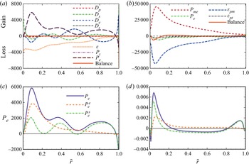
As expected, the balanced TKE budget shown in figure 5(a) depicts that the production of TKE in ET is solely due to the elastic production term ( $P_{e}$). Hence, the Reynolds shear production term (
 $P_t$) is zero. Specifically, except near the outer wall,
 $P_{e}$ has positive values in the entire gap. This signifies increased TKE as a result of a reduction of EPE. Moreover,
 $P_{e}$ achieves its larger values at the inner half-gap, where it is almost balanced by the viscous dissipation
 $\varepsilon$. The viscous and polymer diffusion terms, i.e.
 $D_s$ and
 $D_e$ transport the fluctuating velocity fluids elements near the wall regions to the bulk flow and in turn they alternate as gain and loss terms of relatively small magnitudes. The pressure (
 $D_p$) and turbulent transport (
 $D_t$) terms are approximately zero across the entire gap. The EPE budget shown in figure 5(b) demonstrates that the EPE of polymers is mainly generated by the stretched polymer chains via the mean strain field via
 $P_{me}$. And the dissipation of EPE occurs mainly due to relaxation of stretched polymer chains in the mean flow (via
 $\varepsilon _{pm}$). Moreover, both the largest production and dissipation of EPE occur in the proximity of the inner wall, where rapid stochastic-like spatio-temporal cycles of polymer relaxation/stretch are most intense (see figures 3 and 4). In addition, a small portion of EPE is transformed into TKE to sustain the fluctuating velocities (through
 $P_e$). Consequently, the energy cycle in ET can be summarized as follows: in the presence of the unsteady large-scale diwhirls, polymers are stretched by the mean elongational flow, hence the mean kinetic energy is transformed into EPE, and in turn this energy is transformed into TKE by polymeric stress work; subsequently, the fluctuating fluid velocities produce perturbations to sustain the unsteady character of diwhirls; simultaneously, the entire process is accompanied by dissipation of EPE at the largest flow scale, i.e. by mean flow averaged in time and space (most of the energy) and TKE dissipation occurs by the fluctuating velocities at high-frequency small scales.
(a) The TKE budget for ET at  $Re=0.0001$,
 $Wi=30$: here,
 $D_p$ denotes pressure,
 $D_s$ viscous diffusion,
 $D_e$ polymeric elastic stress and
 $D_t$ the turbulent stress redistribution term of TKE. Also,
 $\varepsilon$ denotes the direct viscous dissipation of TKE,
 $P_t$ is the turbulence shear production term,
 $P_{e}$ is the energy production associated with polymer stretch. (b) The EPE budget for ET at
 $Re=0.0001$,
 $Wi=30$: different lines represent in sequence the polymer energy production induced by the mean (
 $P_{me}$) and fluctuations of elastic stress work (
 $P_{e}$) and dissipation terms associated with the mean (
 $\varepsilon _{pm}$) and fluctuating (
 $\varepsilon _{pt}$) polymer chain motions. The elastic generation term
 $P_{e}$ of the TKE, and its extension (
 $P^{\,e}_{e}=-\nu _p\langle \tau _{rr}^{\prime }s_{rr}^{\prime } + \tau _{\theta \theta }^{\prime }s_{\theta \theta }^{\prime }+\tau _{zz}^{\prime } s_{zz}^{\prime } \rangle$) and shear (
 $P^{\,s}_{e}=-2\nu _p\langle \tau _{r\theta }^{\prime } s_{r\theta }^{\prime }+ \tau _{\theta z}^{\prime }s_{\theta z}^{\prime }+\tau _{rz}^{\prime } s_{rz}^{\prime } \rangle$) parts for (c) ET at
 $Re=0.0001$ and (d) EDT
 $Re=1000$.

The TKE budget analysis of EDT in TC flow and elasto-inertial turbulence (EIT) in channel flows has demonstrated that the elastic production term ( $P_{e}$) makes a dominant contribution to producing TKE, while the Reynolds shear production term (
 $P_t$) is not zero (Dubief, Terrapon & Soria Reference Dubief, Terrapon and Soria2013; Song et al. Reference Song, Lin, Liu, Lu and Khomami2021a). Besides, a qualitative difference in generation of TKE between EDT and pure ET exists. To that end, decomposing
 $P_e$ into its extension (
 $P^{\,e}_{e}$) and shear (
 $P^{\,s}_{e}$) components (see figure 5c,d), in the inner half-gap, shows that
 $P^{\,s}_{e}$ and
 $P^{\,e}_e$ are dominant in
 $P_e$ for EDT and ET, respectively. This is the case for all
 $Re$ of these two turbulent states. Specifically,
 $P^{\,e}_e$/
 $P^{\,s}_e$ corresponds to the work done by the divergent/vortical component of fluctuating elastic stress via the fluctuating extensional/shear flows. This clearly indicates that the coupling of polymer shear stress and the fluctuating shear flows gives rise to EDT. While ET is essentially a turbulent flow that results from significant coupling of rapid cycles of polymer stretch/relaxation and the fluctuating extensional flows realized by the interactions between unsteady diwhirls and propagation of travelling waves.
4. Conclusions
The first 3-D DNS of ET in TC flow of dilute polymeric solutions has enabled quantification of the spatio-temporal dynamics of the flow. Specifically, the simulations qualitatively capture the significant enhancement of flow resistance and a steep power law decay in velocity power spectra observed experimentally. Moreover, the qualitative difference of the turbulence generation mechanism between EDT and pure ET as well as the energy cycle in ET systems have been elucidated via direct examination of the TKE and EPE production, dissipation and transport. The numerical results underscore the importance of 3-D flow structures, namely, axial travelling-like flow patterns in the dynamics of ET. The precise understanding of the effects of travelling waves on the onset of ET still remains an open question that requires detailed investigation. Hence, the present study has paved the way for a mechanistic understanding of polymer induced inertialess turbulence in curvilinear flows.
Funding
This work was supported by the National Natural Science Foundation of China: 12172353, 92052301, 91752110, 11621202, 11572312; and Science Challenge Project TZ2016001; and National Science Foundation CBET0755269. J.S. acknowledges the financial support from the Alexander von Humboldt Research Fellowship Foundation. The calculations were completed on the supercomputing system in the Supercomputing Center at the University of Science and Technology of China.
Declaration of interests
The authors report no conflict of interest.
Appendix. Grid-independence validation
The mesh sizes used in the present DNS are based on our previous numerical studies of inertio-elastic turbulent TC flows (Liu & Khomami Reference Liu and Khomami2013; Song et al. Reference Song, Teng, Liu, Ding, Lu and Khomami2019, Reference Song, Lin, Liu, Lu and Khomami2021a). As demonstrated in our previous grid convergence study, for a wide gap geometry (with the gap width of  $d$, radius ratio
 $\eta =R_i/R_o=1/2=0.5$, the azimuthal computational domain ranges from
 $2{\rm \pi} d$ to
 $4{\rm \pi} d$; hence, it is much smaller than that of the large radius ratio
 $\eta =10.36/11.36=0.912$). To that end, the mesh size of
 $128\times 128\times 256$ for
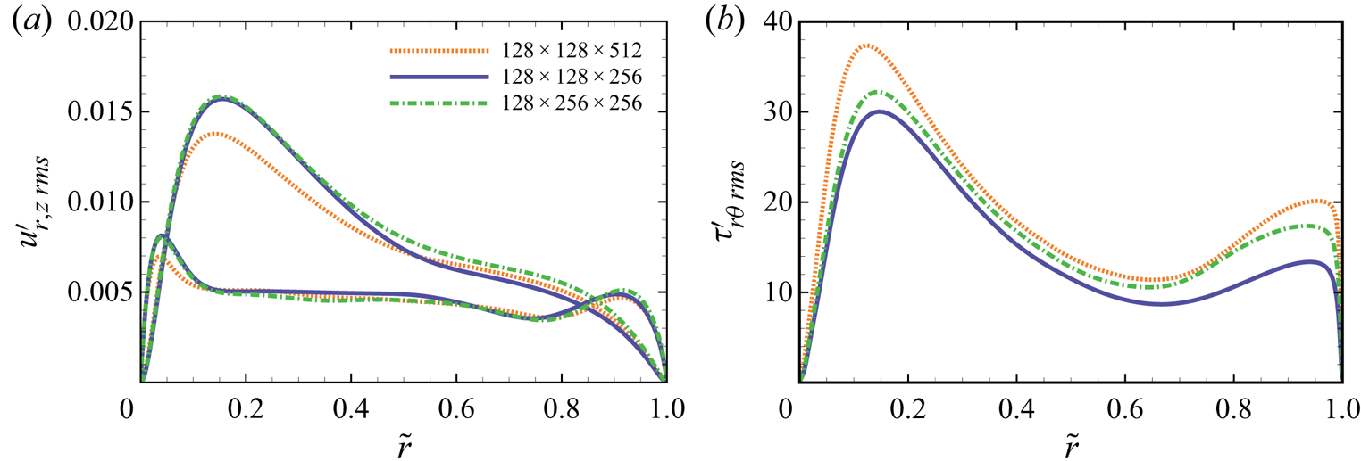
 $r\times \theta \times z$ directions is sufficient to resolve the global response and dynamical behaviour of turbulent TC flows of polymeric solutions considered in this study (Song et al. Reference Song, Teng, Liu, Ding, Lu and Khomami2019, Reference Song, Lin, Liu, Lu and Khomami2021a). In addition, to further scrutinize the accuracy of our simulation results, we have performed a grid-independence check study for the pure ET flow state at
 $Re=0.01$ with
 $Wi=30$. As mentioned in the manuscript, an extremely small time step of
 $0.00025$ is used to avoid numerical instability during the calculation of the highly elastic (
 $El=Wi/Re\geq 3000$) turbulent flows. It should also be noted that this time step is two or three orders of magnitude smaller than the typical DNS of EIT in uni-directional wall bounded shear flows (Lopez, Choueiri & Hof Reference Lopez, Choueiri and Hof2019; Zhu & Xi Reference Zhu and Xi2020). Moreover, this time step is even one order of magnitude smaller than our previous DNS of EDT TC flows (Song et al. Reference Song, Teng, Liu, Ding, Lu and Khomami2019, Reference Song, Lin, Liu, Lu and Khomami2021a,Reference Song, Wan, Liu, Lu and Khomamib). The simultaneous increases of mesh size in the azimuthal and the axial directions makes the calculation tremendously time intensive for our present computational resource. We have only performed two additional simulations with a more refined azimuthal and axial grids (see figure 6). Evidently, the typical turbulent statistics do not show qualitative differences for different mesh sizes. Overall, the most important quantities considered in the present study, i.e. radial and axial velocity and elastic shear stress fluctuations show minor but certainly acceptable quantitative differences with grid refinement. Hence, the mesh sizes used in the present DNS of purely elastic turbulent TC flows are sufficiently refined to capture the purely elastic turbulent dynamics analysed in this study.
Profiles of root-mean-square (r.m.s.) values of (a) radial (upper) and axial (lower) velocity components and (b) polymer shear stress component  $\tau _{r\theta }$ at
 $Re=0.01, Wi=30$ with various mesh sizes.