1 Introduction
Flow-induced vibration (FIV) of elastically mounted bluff bodies is observed in applications as diverse as the oscillation of a flagpole in the wind, the vibration of cooling arrays in nuclear power generators and offshore oil risers. These vibrations can decrease the life of engineering structures and even cause catastrophic failures. Design methods used to avert such effects require a means of predicting their occurrence and characteristics. This has motivated numerous investigations that aim to characterise the fluid–structure system and provide a good understanding of the mechanisms. Surveys of the field are covered in reviews by Griffin, Skop & Koopmann (Reference Griffin, Skop and Koopmann1973), Bearman (Reference Bearman1984), Blevins (Reference Blevins1990), Carberry, Sheridan & Rockwell (Reference Carberry, Sheridan and Rockwell2001), Sarpkaya (Reference Sarpkaya2004), Williamson & Govardhan (Reference Williamson and Govardhan2004), Naudascher & Rockwell (Reference Naudascher and Rockwell2005) and Païdoussis, Price & De Langre (Reference Païdoussis, Price and De Langre2010), amongst others. FIV, on the other hand, could also find applications in energy harvesting and vibration control. Comprehensive reviews on this topic are given by Xiao & Zhu (Reference Xiao and Zhu2014) and Young, Lai & Platzer (Reference Young, Lai and Platzer2014).
There are two body oscillator phenomena typical of FIV: vortex-induced vibration (VIV) and transverse galloping (see Naudascher & Rockwell Reference Naudascher and Rockwell2005). VIV is caused by vortex shedding in the wake of a body that then causes structural vibration due to the spatially oscillating pressure field associated with the shed vortices. Since the pioneering study by Feng (Reference Feng1968), VIV has been extensively investigated using the canonical model of an elastically mounted rigid circular cylinder that is free or forced to oscillate transversely in a free stream (Bishop & Hassan Reference Bishop and Hassan1964; Bearman Reference Bearman1984, Reference Bearman2011; Williamson & Roshko Reference Williamson and Roshko1988; Govardhan & Williamson Reference Govardhan and Williamson2000; Carberry et al. Reference Carberry, Sheridan and Rockwell2001; Morse & Williamson Reference Morse and Williamson2009; Zhao et al. Reference Zhao, Leontini, Lo Jacono and Sheridan2014a ).
While the axial symmetry of a circular cross-section enables VIV to be studied independently from other forms of FIV (i.e. galloping), it should be noted that VIV can still occur under certain conditions (e.g. mass and damping ratios) and dominate over a range of reduced velocity when the axial symmetry is broken, as demonstrated by Corless & Parkinson (Reference Corless and Parkinson1988), Nemes et al. (Reference Nemes, Zhao, Lo Jacono and Sheridan2012) and Zhao et al. (Reference Zhao, Leontini, Lo Jacono and Sheridan2014b
). In such cases, however, the body may also be subjected to transverse galloping. Galloping is categorised as movement-induced excitation (MIE) by Naudascher & Rockwell (Reference Naudascher and Rockwell2005). It commonly occurs when the cylindrical body is not axisymmetric, making it aerodynamically unstable to transverse oscillations (Blevins Reference Blevins1990; Naudascher & Rockwell Reference Naudascher and Rockwell2005; Païdoussis et al.
Reference Païdoussis, Price and De Langre2010). Generally, galloping is characterised by oscillations with amplitudes increasing monotonically with flow speed and frequencies much lower than that of vortex shedding (Bearman et al.
Reference Bearman, Gartshore, Maull and Parkinson1987); for instance, iced electrical transmission cables were observed to oscillate with low frequencies and amplitudes of the order of
 $100$
diameters in winds (see Den Hartog Reference Den Hartog1932). The galloping response is attributable to the asymmetric pressure distribution over the body that is created by the changing instantaneous angle of attack between the flow and the body. VIV and galloping need not occur mutually exclusively; their occurrence depends on the flow and structural properties. In fact, the two FIV phenomena may occur in the same flow regimes, as shown in Corless & Parkinson (Reference Corless and Parkinson1988), Nemes et al. (Reference Nemes, Zhao, Lo Jacono and Sheridan2012) and Zhao et al. (Reference Zhao, Leontini, Lo Jacono and Sheridan2014b
). Nemes et al. (Reference Nemes, Zhao, Lo Jacono and Sheridan2012) and Zhao et al. (Reference Zhao, Leontini, Lo Jacono and Sheridan2014b
) have shown that large amplitude response regions can result from the interaction between VIV and galloping.
The present study introduces asymmetry into the system via actuating the body through the application of forced rotation to an elastically mounted circular cylinder. Similar mechanical configurations could have practical applications in offshore engineering, where long slender rotating shafts are exposed to varying flow in an ocean current. Understanding the behaviour of a rotating cylinder undergoing VIV may enable behavioural prediction of similar mechanical systems, and could contribute to energy harvesting applications and FIV control, given the possibility of enhancing or suppressing the vibrations.
Rigidly mounted (non-oscillating) circular cylinders undergoing forced rotation in a cross-flow have also been the subject of studies and reviews over the past century (e.g. Tietjens & Prandtl Reference Tietjens and Prandtl1957; Swanson Reference Swanson1961; Coutanceau & Ménard Reference Coutanceau and Ménard1985; Mittal & Kumar Reference Mittal and Kumar2003; Rao et al.
Reference Rao, Leontini, Thompson and Hourigan2013), due to the potential for wake manipulation. Different wake regimes have been identified in these previous studies that are found to depend on the non-dimensional rotation rate of the cylinder, defined as the ratio between the cylinder surface (
 $|\unicode[STIX]{x1D6FA}|$
) and free-stream (
 $U$
) velocities, namely
 $\unicode[STIX]{x1D6FC}=|\unicode[STIX]{x1D6FA}|D/(2U)$
, where
 $D$
is the diameter of the cylinder. Asymmetric vortex shedding occurs in the wake for
 $0<\unicode[STIX]{x1D6FC}\lesssim 2$
; and many experimental and numerical works have shown this alternating vortex shedding over a wide range of Reynolds number (e.g. Coutanceau & Ménard Reference Coutanceau and Ménard1985; Badr et al.
Reference Badr, Coutanceau, Dennis and Ménard1990; Kang, Choi & Lee Reference Kang, Choi and Lee1999; He et al.
Reference He, Glowinski, Metcalfe, Nordlander and Periaux2000; Stojković, Breuer & Durst Reference Stojković, Breuer and Durst2002; Mittal & Kumar Reference Mittal and Kumar2003; Rao et al.
Reference Rao, Leontini, Thompson and Hourigan2013). Over a small range of
 $\unicode[STIX]{x1D6FC}\geqslant 4$
there is a secondary region of wake unsteadiness, comprising low-frequency one-sided vortices, as shown by Mittal & Kumar (Reference Mittal and Kumar2003), Stojković et al. (Reference Stojković, Schön, Breuer and Durst2003) and Pralits, Brandt & Giannetti (Reference Pralits, Brandt and Giannetti2010). Numerical simulations have shown that the critical Reynolds number of the secondary instability associated with the spanwise undulation of the von Kármán vortices increases with Reynolds number (El Akoury et al.
Reference El Akoury, Braza, Perrin, Harran and Hoarau2008; Rao et al.
Reference Rao, Radi, Leontini, Thompson, Sheridan and Hourigan2015). Depending on
 $\unicode[STIX]{x1D6FC}$
and
 $Re$
, there exist a number of steady and unsteady wake modes (Pralits, Giannetti & Brandt Reference Pralits, Giannetti and Brandt2013; Rao et al.
Reference Rao, Leontini, Thompson and Hourigan2013, Reference Rao, Radi, Leontini, Thompson, Sheridan and Hourigan2015).
Bourguet & Lo Jacono (Reference Bourguet and Lo Jacono2014, hereafter BL14) appear to have been the first to conduct a low-
 $Re$
numerical study of an elastically mounted circular cylinder undergoing forced rotation. This study was undertaken at
 $Re=100$
over a parameter space spanning the reduced velocity range
 $4\leqslant U^{\ast }\leqslant 34$
and the rotation rate range
 $0\leqslant \unicode[STIX]{x1D6FC}\leqslant 4$
. Here, the reduced velocity is defined by
 $U^{\ast }=U/(f_{nw}D)$
, with
 $U$
the free-stream velocity,
 $f_{nw}$
the natural frequency of the system in quiescent water and
 $D$
the cylinder diameter. They found that the time-averaged displacement of the cylinder tended to increase with
 $\unicode[STIX]{x1D6FC}$
, as did the time-averaged transverse lift-force coefficient. Non-negligible oscillations (i.e.
 $A^{\ast }\equiv A/D\geqslant 0.05$
, with
 $A$
the oscillation amplitude) occurred in both the unstable (
 $\unicode[STIX]{x1D6FC}<1.8$
) and stable (
 $1.8\leqslant \unicode[STIX]{x1D6FC}\leqslant 3.75$
) flow regimes, based on whether the wake of a non-oscillating rotating cylinder had an unsteady or steady wake. For
 $\unicode[STIX]{x1D6FC}\leqslant 3.75$
, the peak amplitude response was found to increase with
 $\unicode[STIX]{x1D6FC}$
, and the largest peak amplitude was observed to be
 $1.9D$
at
 $(\unicode[STIX]{x1D6FC},U^{\ast })=(3.75,13)$
, three times the peak response of the non-rotating case. Also, they found that large oscillations of the rotating cases were associated with wake–body synchronisations, similar to the lock-in of a non-rotating cylinder. In addition, BL14 examined the wake patterns associated with the effects of cylinder rotation. They observed wake patterns (i.e. 2S,
 $\text{P}+\text{S}$
) that have commonly been reported in previous VIV studies of a non-rotating cylinder (e.g. Williamson & Roshko Reference Williamson and Roshko1988; Blackburn & Henderson Reference Blackburn and Henderson1999; Mittal & Kumar Reference Mittal and Kumar2003; Jauvtis & Williamson Reference Jauvtis and Williamson2004; Dahl et al.
Reference Dahl, Hover, Triantafyllou, Dong and Karniadakis2007). However, they also identified a novel T+S wake pattern composed of a triplet of vortices and a single vortex shed per oscillation cycle, which was attributable to the largest amplitude response.
Zhao, Cheng & Lu (Reference Zhao, Cheng and Lu2014c
) numerically studied both one- and two-degree-of-freedom (1- and 2-DOF) systems with imposed cylinder rotation, again at low Reynolds numbers. At a constant
 $\unicode[STIX]{x1D6FC}$
, they observed hysteretic regions in the amplitude response. These regions were similar to those of a non-rotating circular cylinder undergoing VIV when monotonically increasing and then decreasing
 $U^{\ast }$
. The 2-DOF studies showed significant differences in vibration response between a non-rotating cylinder and cylinders rotating at
 $\unicode[STIX]{x1D6FC}=0.5$
and
 $1.0$
.
More recently, Seyed-Aghazadeh & Modarres-Sadeghi (Reference Seyed-Aghazadeh and Modarres-Sadeghi2015, hereafter SM15) experimentally studied VIV of a rotating cylinder at relatively low Reynolds numbers (
 $Re=350$
–
 $1000$
). Results were presented showing the vibration response and corresponding flow visualisations in the wake. Of interest, the amplitude response was found to increase only marginally with rotation rate over that of a non-rotating cylinder undergoing VIV, from
 $A^{\ast }\simeq 0.5$
to
 $A^{\ast }\simeq 0.6$
at
 $\unicode[STIX]{x1D6FC}\simeq 2.4$
, and dropping away after this. This result, showing only a minimal effect of rotation, is distinctly different from the previous numerical studies of BL14 and Zhao et al. (Reference Zhao, Cheng and Lu2014c
).
In summary, previous parameter space studies have investigated the vibration responses and wake modes for both the 1-DOF and 2-DOF oscillation cases, but only at relatively low Reynolds number. Some of these studies appear to be at least superficially contradictory, in terms of amplitude response with rotation rate, peak response and the reduced velocity ranges for significant vibration response. The present work is an attempt to study this problem over a higher-Reynolds-number range, where the VIV response is likely to be less sensitive to Reynolds-number variations. Thus, the findings are likely to be more applicable to typical physical and/or industrial applications, where Reynolds numbers are generally higher. This investigation also aims to study the vibration response and wake structure over a wider range of parameter space (
 $U^{\ast }$
,
 $Re$
and
 $\unicode[STIX]{x1D6FC}$
) than previous experimental work.
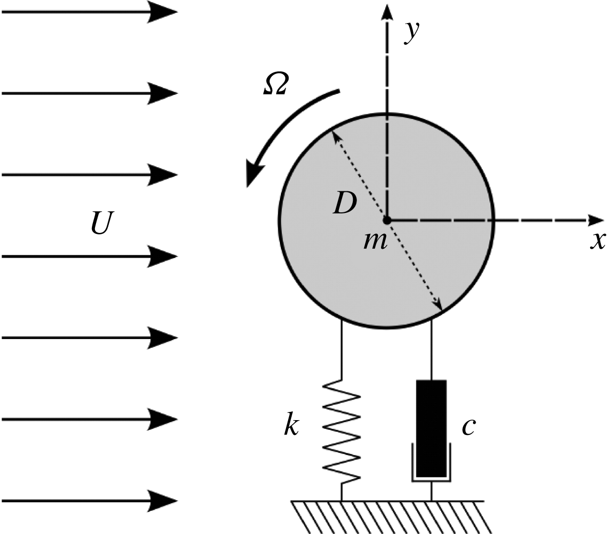
Definition sketch for the transverse FIV of a rotating cylinder. The hydroelastic system is simplified as a 1-DOF system constrained to move in the cross-flow direction. The axis of rotation is transverse to both the flow direction (
 $x$
-axis) and the oscillation axis (
 $y$
-axis). Here,
 $U$
is the free-stream velocity,
 $k$
the spring constant,
 $D$
the cylinder diameter,
 $m$
the oscillating mass,
 $c$
the structural damping and
 $\unicode[STIX]{x1D6FA}$
the angular velocity.
The remainder of the paper is structured as follows. The experimental methodology, including the fluid–structure system modelling, experimental details and a validation study, is presented in § 2. The results are presented in § 3, followed by discussion in § 3.4. Finally, conclusions are drawn in § 4.
2 Experimental methodology
2.1 Fluid–structure system modelling
A schematic of the fluid–structure system is presented in figure 1. The elastically mounted cylinder is free to oscillate in only one direction transverse to the oncoming free stream. The governing equation of motion can be written as
 $$\begin{eqnarray}m\ddot{y} +c{\dot{y}}+ky=F_{y},\end{eqnarray}$$
where
 $F_{y}$
represents the fluid force in the transverse direction,
 $m$
is the total oscillating mass of the system,
 $c$
is the structural damping of the system,
 $k$
is the spring constant and
 $y$
is the displacement in the transverse direction.
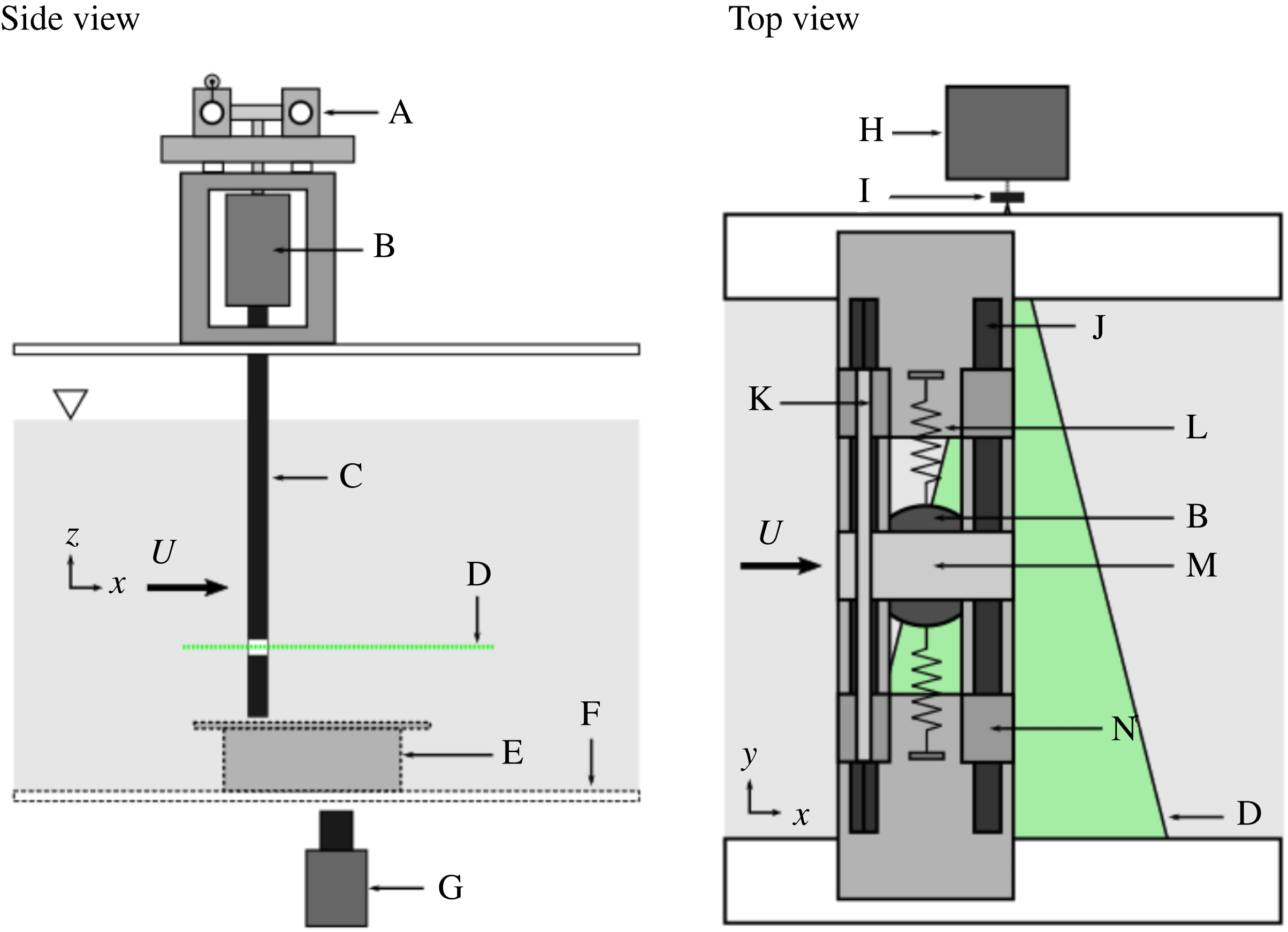
In the present experiments, the hydroelastic system was modelled based on a low-friction air bearing system in conjunction with the recirculating free-surface water channel of the Fluids Laboratory for Aeronautical and Industrial Research (FLAIR), Monash University. The test section of the water channel has dimensions of 600 mm in width, 800 mm in depth and 4000 mm in length. The free-stream velocity in the present experiments could be varied continuously over the range
 $0.05\leqslant U\leqslant 0.45~\text{m}~\text{s}^{-1}$
. The free-stream turbulence level was less than
 $1\,\%$
. Figure 2 shows a schematic of the experimental set-up, while figure 3 shows an actual photograph of the experimental rig to clarify details. The air-bearing system positioned above the water channel provided low structural damping and constrained the body motion to the cross-flow (transverse) direction. Structural stiffness of the oscillating system was controlled by stainless-steel extension springs attached to both sides of the support carriage and the base of the air-bearing system. More details of this hydroelastic system can be found in Nemes et al. (Reference Nemes, Zhao, Lo Jacono and Sheridan2012) and Zhao et al. (Reference Zhao, Leontini, Lo Jacono and Sheridan2014a
,Reference Zhao, Leontini, Lo Jacono and Sheridan
b
).
Schematic of the experiment (not scaled): A, low-friction air-bearing system; B, cylinder rotation device with built-in motor and optical rotary encoder; C, 30 mm test cylinder with transparent laser window; D, 532 nm laser sheet; E, transparent end plate; F, transparent test section window; G, camera; H, 532 nm laser; I, cylindrical lens; J, carbon shaft; K, linear voltage differential transformer (LVDT); L, stainless-steel springs; M, support carriage; N, air-bearing bushing.
The cylinder model used was precision-machined from aluminium tubing and had a diameter of
 $D=30\pm 0.01~\text{mm}$
. The immersed length of the cylinder was
 $L=614~\text{mm}$
, giving an aspect ratio of
 $L/D\simeq 20.5$
. To reduce end effects of the cylinder and to promote parallel vortex shedding, a conditioning platform was placed under the cylinder, and the gap between the cylinder end and the platform surface was set to approximately 1 mm
 $(0.03D)$
(see Khalak & Williamson Reference Khalak and Williamson1997, Reference Khalak and Williamson1999; Zhao et al.
Reference Zhao, Leontini, Lo Jacono and Sheridan2014a
,Reference Zhao, Leontini, Lo Jacono and Sheridan
b
).
The cylinder rotation rate is defined as the ratio of the cylinder surface speed to the free-stream velocity, namely
 $\unicode[STIX]{x1D6FC}=|\unicode[STIX]{x1D6FA}|D/(2U)$
. The rotation speed of the cylinder was controlled using a motion control system manufactured by Parker Hannifin (USA) consisting of a controller (model 6K2), a motor drive (model E-DC) and a miniature low-voltage micro-stepping motor (model LV172) with a resolution of 25 000 steps per revolution.
The total oscillating mass, including the cylinder model, motor assembly and moving components of the air-bearing system, was
 $m=2503.6~\text{g}$
and the displaced mass of the fluid was
 $m_{d}=433.1~\text{g}$
, resulting in a mass ratio of
 $m^{\ast }=m/m_{d}=5.78$
. The natural frequencies of the system and the structural damping in both air and water were determined by conducting free-decay tests individually in air and in quiescent water. The natural frequency in quiescent water was found to be
 $f_{nw}=0.671~\text{Hz}$
. The structural damping ratio in air was
 $\unicode[STIX]{x1D701}_{air}\simeq c/(2\sqrt{km})=4.1\times 10^{-3}$
.
The cylinder flexed slightly under large body oscillations, which resulted in a minor deviation between the cross-sectional centroid position of the cylinder at the top, where there was minimal cylinder flexing, and the centroid position of the cylinder at the bottom, where transverse deflection due to flexing was largest. This was quantified by measuring the difference in the centroid positions at the top and bottom using a linear variable differential transformer (LVDT) and a high-speed camera (see § 2.2 for further details), respectively. In the worst case (
 $U^{\ast }=6.0$
) the deviation was measured as
 ${\sim}0.1D$
, while the peak-to-peak oscillation measured
 $2.8D$
, i.e. approximately 3.5 %. Alternatively, this represented a deflection of the cylinder over its length of less than
 $0.3^{\circ }$
.
A photograph showing the experimental rig used in the present study.

2.2 Data acquisition and processing methods
The data acquisition and the control of the free-stream velocity and motor rotation speed over the
 $U^{\ast }$
–
 $\unicode[STIX]{x1D6FC}$
parameter space were automated using customised LabVIEW (National Instruments, USA) programs. The reduced velocity was varied over the range
 $2.5\leqslant U^{\ast }\leqslant 14$
in increments between 0.25 and 1 (depending on structural response regimes). The corresponding Reynolds-number range was
 $1132\leqslant Re\leqslant 6313$
. Note that the Reynolds number is defined by
 $Re=UD/\unicode[STIX]{x1D708}$
, where
 $\unicode[STIX]{x1D708}$
is the kinematic viscosity of the fluid. Fluctuations in the kinematic viscosity with temperature were considered minimal, with temperature fluctuations of less than
 $\pm 0.5\,^{\circ }\text{C}$
while the experiments were undertaken. The cylinder rotation rate was varied over the range
 $0\leqslant \unicode[STIX]{x1D6FC}\leqslant 4.2$
in increments of
 $0.05$
.
The body displacement was measured using a non-contact (magnetostrictive) LVDT. The accuracy of the LVDT was within
 $\pm 0.01\,\%$
of the 250 mm range available (see Zhao et al.
Reference Zhao, Leontini, Lo Jacono and Sheridan2014a
,Reference Zhao, Leontini, Lo Jacono and Sheridan
b
). The rotation speed was measured using a digital optical rotary encoder (model E5-1000, US Digital, USA) with a resolution of 4000 counts per revolution. The sampling frequency for all measurements was set to 100 Hz. For each point in the
 $U^{\ast }$
–
 $\unicode[STIX]{x1D6FC}$
parameter space, the structural response was measured for at least 300 s, which amounted to more than
 $300$
oscillation cycles. Sufficient transition time (180 s) was allowed between changing either
 $\unicode[STIX]{x1D6FC}$
or
 $U^{\ast }$
to enable the VIV response to fully develop before recording the signal sequences. To remove high-frequency electrical noise, a low-pass Butterworth filter of order
 $4$
with a cut-off frequency of 2 Hz was applied to all analogue signals prior to further processing. Fast Fourier transforms (FFTs) were used to extract body oscillation frequencies from the LVDT signals.
The particle image velocimetry (PIV) technique was employed to capture flow structures in the near wake of the cylinder. The flow was seeded with hollow microspheres (Sphericel 110P8, Potters Industries Inc.) having a normal diameter of
 $13~\unicode[STIX]{x03BC}\text{m}$
and a specific weight of
 $1.1~\text{g}~\text{m}^{-3}$
. The particles were illuminated by a 2 mm thick horizontal planar laser sheet from two miniature Ng:YAG pulse lasers (Continuum Minilite II, USA), while imaging was performed using a high-speed camera (Dimax S4, PCO AG, Germany) with a resolution of 2016 pixel
 $\times$
2016 pixel. The camera was equipped with a 50 mm lens (Nikon Corporation, Japan), giving a magnification of
 $9.71~\text{pixel}~\text{mm}^{-1}$
for the field of view of interest. The PIV image pairs were captured at 14 Hz using a TTL pulse generator. For each PIV imaging location in the
 $U^{\ast }$
–
 $\unicode[STIX]{x1D6FC}$
space,
 $3140$
image pairs were recorded for quantitative analysis. The imaging data were processed using validated in-house PIV software developed by Fouras, Lo Jacono & Hourigan (Reference Fouras, Lo Jacono and Hourigan2008). More details of the method used for identifying the wake structures are further provided in § 3.2.
2.3 Validation
The vibration response of a non-rotating circular cylinder undergoing VIV is compared against previous work by Khalak & Williamson (Reference Khalak and Williamson1997, Reference Khalak and Williamson1999) and Zhao et al. (Reference Zhao, Leontini, Lo Jacono and Sheridan2014b
) in figure 4. Figure 4(a) presents the amplitude response as a function of reduced velocity and shows the current experimental configuration produces non-rotating VIV results in good agreement with previous VIV studies. Here, it is important to note the effect of the mass ratio, which is necessarily higher here than for some of the comparison studies because of the added weight arising from the motor assembly. At the lowest
 $m^{\ast }$
achievable, of
 $m^{\ast }=5.78$
, the typical VIV amplitude response branches of a non-rotating cylinder are seen. The initial branch exists for
 $U^{\ast }<4.8$
. At
 $m^{\ast }=5.78$
, the upper branch covers the range
 $U^{\ast }=4.8{-}6.4$
; the lower response branch lies within the range
 $6.4\leqslant U^{\ast }\leqslant 9.5$
; and the desynchronised region occurs for
 $U^{\ast }>9.5$
. Previous studies by Khalak & Williamson (Reference Khalak and Williamson1997) and Zhao et al. (Reference Zhao, Leontini, Lo Jacono and Sheridan2014b
) at
 $m^{\ast }=2.4$
showed a peak amplitude response of
 $A^{\ast }\approx 0.95$
. The mean of the highest
 $10\,\%$
of peak amplitude response (
 $A_{10}^{\ast }$
) of the current system is
 $A_{10}^{\ast }=0.82$
. This agrees with previous studies on the effects of mass and damping. As the mass and damping ratios are increased, the magnitude of the amplitude response decreases and the range of
 $U^{\ast }$
over which the system self-excites reduces (Feng Reference Feng1968). A hysteretic transition between the initial and upper branch occurs at
 $U^{\ast }\approx 4.8$
and is accompanied by a jump in
 $A_{10}^{\ast }$
from
 $0.25$
to
 $0.79$
. The transition from the upper to lower branch causes a reduction in
 $A_{10}^{\ast }$
from
 $0.78$
to
 $0.55$
, and the desynchronisation of the system at
 $U^{\ast }\approx 9.5$
is accompanied by a drop in
 $A_{10}^{\ast }$
from
 $0.54$
to
 ${\sim}0.07$
. This comparison with results from previous literature shows that the current air-bearing system reproduces an amplitude response consistent with previous careful studies.
Vibration response of a non-rotating circular cylinder undergoing VIV. (
 $a$
) The normalised amplitude response (
 $A^{\ast }$
) as a function of reduced velocity (
 $U^{\ast }$
): ●, the mean of the highest
 $10\,\%$
of oscillation amplitude in the present study with
 $m^{\ast }=5.78$
and
 $\unicode[STIX]{x1D701}=0.0041$
; ▫, results from Zhao et al. (Reference Zhao, Leontini, Lo Jacono and Sheridan2014b
) with
 $m^{\ast }=2.4$
and
 $\unicode[STIX]{x1D701}=0.00243$
; ▵, results from Khalak & Williamson (Reference Khalak and Williamson1997) with
 $m^{\ast }=2.4$
and
 $\unicode[STIX]{x1D701}=0.0045$
; ▿, results from Khalak & Williamson (Reference Khalak and Williamson1999) with
 $m^{\ast }=10.3$
and
 $\unicode[STIX]{x1D701}=0.00165$
. The vertical dashed lines represent the boundaries of branches for the present study. (
 $b$
) A PSD contour map of
 $A^{\ast }$
as a function of
 $f^{\ast }$
and
 $U^{\ast }$
. Essentially normalised power spectra are assembled together horizontally to construct this map. Note that the PSD is normalised by the peak value at each
 $U^{\ast }$
.

Figure 4(b) presents a power spectral density (PSD) contour plot of the normalised cylinder displacement as a function of the normalised frequency response
 $f^{\ast }$
and reduced velocity
 $U^{\ast }$
. This consists of individual vertically aligned greyscale-coded power spectra for each
 $U^{\ast }$
stacked together horizontally to show the frequency response of the system, with darker regions representing frequencies of higher power. The narrowness or broadness of the spectral peaks is also clear from the colour gradation. The variation of the shedding frequency ratio (
 $f_{sh}/f$
) with
 $U^{\ast }$
is plotted as a dot-dashed line in figure 4(b) to highlight
 $U^{\ast }$
regions where
 $f\approx f_{sh}$
. To highlight
 $U^{\ast }$
ranges where
 $f$
locks to
 $f_{nw}$
(i.e.
 $f\approx f_{nw}$
), the
 $f^{\ast }=1$
curve is shown as a dotted line in figure 4(b). The body’s frequency response (
 $f$
) follows the shedding frequency (
 $f\approx f_{sh}$
) until the end of the initial amplitude response branch, where it begins to bend towards
 $f_{nw}$
and subsequently lock in to it (
 $f\approx f_{nw}$
). The frequency response remains synchronised throughout the upper and lower amplitude response branches until the desynchronised region is reached. At that point, the body frequency response deviates from
 $f_{nw}$
, returning to follow
 $f_{sh}$
, although there is still a broad spectral peak close to the natural shedding frequency. For the current experiment, the mean Strouhal number, defined by
 $St=f_{sh}D/U$
, was measured as
 $St\approx 0.215$
for the
 $Re$
range investigated; this agrees with the known
 $St$
value in the same
 $Re$
range.
3 Results
The vibration response and time-averaged position of the cylinder are presented in § 3.1, and the wake modes and structure are explored in § 3.2. A specific section is devoted to the wake state in the upper branch where intermittent behaviour is observed to occur (§ 3.3), prior to a short discussion comparing current results with those from previous related studies in the following section (§ 3.4).
3.1 Vibration response
The time-averaged displacement of the cylinder from its non-rotating neutral position (
 $\bar{y}$
) is discussed first, followed by the observed vibration response, i.e. the oscillation amplitude and frequency response, as
 $U^{\ast }$
and
 $\unicode[STIX]{x1D6FC}$
are varied. The oscillations observed in the current study are typically broadly periodic although there is some variation of the waveform from cycle to cycle. When a cylindrical body is rotated about its axis in a fluid flow, an asymmetric pressure distribution is generated. This uneven pressure distribution is the result of fluid being accelerated by the body rotation on the leeward side, and decelerated with flow separation from the body on the windward side. This is generally known as the Magnus effect, and it has been extensively studied over the past century (e.g. Tietjens & Prandtl Reference Tietjens and Prandtl1957; Coutanceau & Ménard Reference Coutanceau and Ménard1985; Badr et al.
Reference Badr, Coutanceau, Dennis and Ménard1990; Kang et al.
Reference Kang, Choi and Lee1999; He et al.
Reference He, Glowinski, Metcalfe, Nordlander and Periaux2000; Stojković et al.
Reference Stojković, Breuer and Durst2002; Mittal & Kumar Reference Mittal and Kumar2003; Rao et al.
Reference Rao, Leontini, Thompson and Hourigan2013). A net transverse force is generated by the asymmetric pressure distribution. The magnitude of the force increases with
 $\unicode[STIX]{x1D6FC}$
; therefore, it is expected that, at any
 $U^{\ast }$
, an increase in
 $\unicode[STIX]{x1D6FC}$
will result in an increase in the magnitude of
 $\bar{y}$
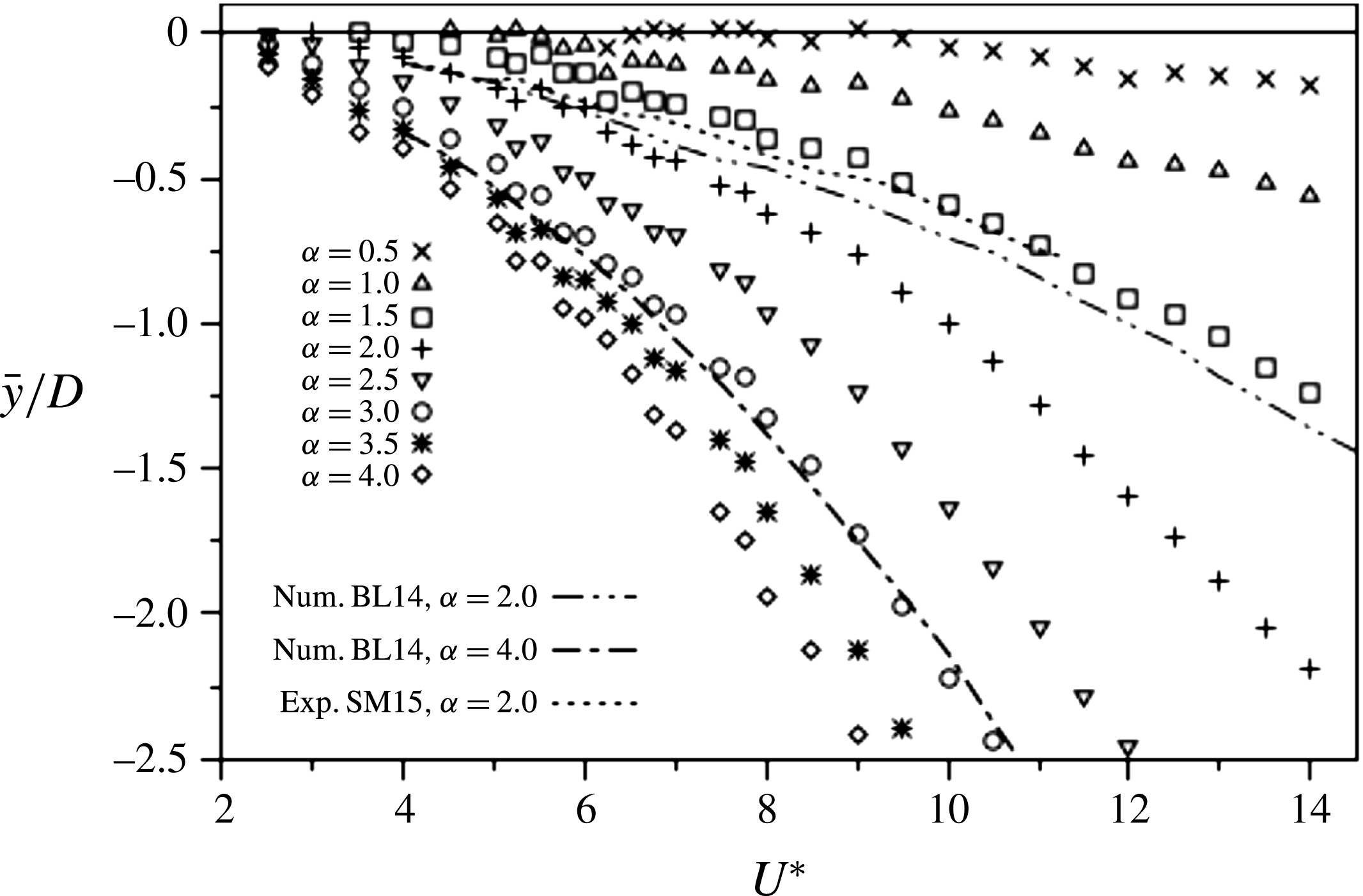
. Figure 5 presents
 $\bar{y}$
as a function of
 $U^{\ast }$
at varying
 $\unicode[STIX]{x1D6FC}$
. This shows that
 $\bar{y}$
increases in magnitude with
 $\unicode[STIX]{x1D6FC}$
as expected due to the increase in the mean cross-flow force. This general behaviour agrees with rotating VIV results from low-Reynolds-number (
 $Re=100$
) simulations of BL14, although the current experimental offsets are generally larger than the numerical ones. In figure 5, the
 $Re=100$
numerical predictions for
 $\unicode[STIX]{x1D6FC}=2.0$
(dashed) and
 $\unicode[STIX]{x1D6FC}=4.0$
(solid) are overlaid for comparison. The measured experimental variation of SM15 for
 $\unicode[STIX]{x1D6FC}=2.0$
is also overlaid (dot-dashed line). This is closer to the
 $Re=100$
numerical result than the present variation, perhaps consistent with the lower-Reynolds-number range (
 $Re=350$
–
 $1000$
) of that study.
The time-averaged displacement of the cylinder (
 $\bar{y}$
) as a function of reduced velocity (
 $U^{\ast }$
) at different rotation rates (
 $\unicode[STIX]{x1D6FC}$
). Numerical predictions BL14 for
 $Re=100$
at
 $\unicode[STIX]{x1D6FC}=2.0$
and
 $4.0$
are shown by the dot-dashed lines. The dotted line shows experimental results of SM15 at
 $Re=350$
–
 $1000$
,
 $\unicode[STIX]{x1D6FC}=2.0$
for comparison.
The vibration response of an elastically mounted circular cylinder undergoing constant rotation as a function of reduced velocity (
 $U^{\ast }$
) at different rotation rates (
 $\unicode[STIX]{x1D6FC}$
). (a) The normalised amplitude response (
 $A_{10}^{\ast }$
). (b) The normalised frequency response (
 $f^{\ast }$
). Approximate fits to cases
 $\unicode[STIX]{x1D6FC}=0$
,
 $1.0$
,
 $2.0$
and
 $3.0$
are shown by the labelled dashed lines.
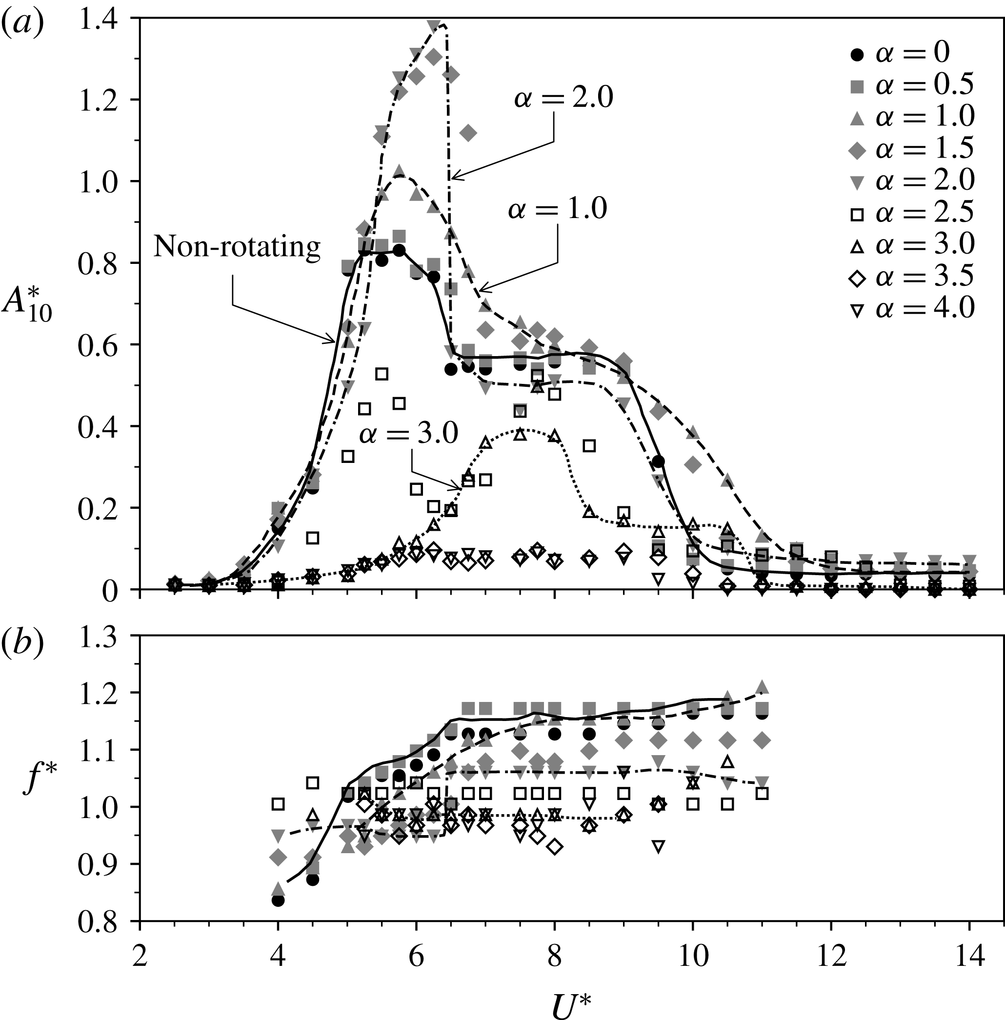
The oscillatory component of the motion of the cylinder is characterised in figures 6 and 7. Figure 6 shows how the vibration response varies as a function of
 $U^{\ast }$
. The means of the highest
 $10\,\%$
of normalised amplitude response peaks (
 $A_{10}^{\ast }$
) about their time-averaged positions (
 $\bar{y}$
) are presented as a function of
 $U^{\ast }$
and
 $\unicode[STIX]{x1D6FC}$
in figure 6(a). The amplitude response for a number of different cases (
 $\unicode[STIX]{x1D6FC}=0$
, 1.0, 2.0 and 3.0) are highlighted by dashed lines to help clarify the overall behaviour with rotation rate. Large amplitude oscillations are observed over a broad range of
 $U^{\ast }$
and
 $\unicode[STIX]{x1D6FC}$
. The peak amplitude first increases as the rotation rate is increased from
 $\unicode[STIX]{x1D6FC}=0$
, while beyond
 $\unicode[STIX]{x1D6FC}=2$
there is a decrease in the peak response. Overall, the amplitude response is similar to the non-rotating VIV case for
 $\unicode[STIX]{x1D6FC}\leqslant 2.0$
. While distorted by the effects of rotation, the three amplitude response branches, i.e. the initial, upper and lower branches, can be clearly identified. Over the rotation rate range
 $0<\unicode[STIX]{x1D6FC}\leqslant 1.5$
, an increase in
 $\unicode[STIX]{x1D6FC}$
results in an increase in peak amplitude response, transitions between the upper and lower branch and the desynchronisation become less distinct, and the width of the
 $U^{\ast }$
range over which excitation occurs increases. For rotation rates between
 $1.5<\unicode[STIX]{x1D6FC}\leqslant 2.0$
, the peak amplitude increases to higher values than seen at lower
 $\unicode[STIX]{x1D6FC}$
. The transition between upper and lower branches is abrupt, but the range of
 $U^{\ast }$
at which excitation occurs is similar to that of a non-rotating cylinder. Up to a rotation rate of
 $\unicode[STIX]{x1D6FC}\approx 2.0$
, the
 $U^{\ast }$
range corresponding to the amplitude peak increases with
 $\unicode[STIX]{x1D6FC}$
. In the range
 $2<U^{\ast }\leqslant 3$
, the amplitude response decreases significantly, and the response curve shape no longer resembles that seen for non-rotating VIV. Instead of the typical two- or three-branch response, in this range of
 $\unicode[STIX]{x1D6FC}$
these are replaced with a twin-peak (
 $\unicode[STIX]{x1D6FC}=2.5$
) and a small single-peak (
 $\unicode[STIX]{x1D6FC}=3.0$
) response. Also, the range of reduced velocity at which excitation occurs becomes narrower. For
 $\unicode[STIX]{x1D6FC}>3.0$
, body excitation is minimal.
The vibration response of an elastically mounted circular cylinder undergoing constant rotation as a function of rotation rate (
 $\unicode[STIX]{x1D6FC}$
) at selected reduced velocities (
 $U^{\ast }$
). In each reduced velocity case, panel (i) is the normalised amplitude response (
 $A_{10}^{\ast }$
) and panel (ii) is the PSD contour of the normalised reduced velocity (
 $f^{\ast }$
) normalised by the peak power. The horizontal solid lines in panels (ii) indicate
 $f^{\ast }=1$
(or
 $f=f_{nw}$
). The vertical dashed lines highlight features of interest discussed in the text.

The normalised frequency response about its time-averaged position is presented as a function of
 $U^{\ast }$
and
 $\unicode[STIX]{x1D6FC}$
in figure 6(b). As for the amplitude response curves, the frequency variations for the non-rotating case and
 $\unicode[STIX]{x1D6FC}=1.0,~2.0$
and
 $3.0$
are highlighted by dashed lines. For the non-rotating case, again there is good agreement with previous VIV studies. The frequency response follows the non-rotating VIV response and the response globally decreases with increasing
 $\unicode[STIX]{x1D6FC}$
. This is also in good agreement with the numerical results found by BL14 and experiments of SM15.
A study of the vibration response at fixed
 $\unicode[STIX]{x1D6FC}$
increments can better show the effects of rotation on the vibration response and how each
 $\unicode[STIX]{x1D6FC}$
increment compares to the non-rotating VIV case over the tested
 $U^{\ast }$
range. The normalised vibration response about its time-averaged position at several
 $U^{\ast }$
of interest were selected and are presented as a function of
 $\unicode[STIX]{x1D6FC}$
and
 $U^{\ast }$
in figure 7. The selection of these values of
 $U^{\ast }$
was based on how each represents the vibration response at similar
 $U^{\ast }$
, and how well these cases show the response progression with increasing
 $U^{\ast }$
. Figure 7(ai) shows
 $A_{10}^{\ast }$
as a function of
 $\unicode[STIX]{x1D6FC}$
at
 $U^{\ast }=4.00$
. At this reduced velocity, the amplitude response is small (
 $A^{\ast }\lesssim 0.2$
) with increased rotation further suppressing oscillations beyond
 $\unicode[STIX]{x1D6FC}=2.3$
. Figure 7(
 $a$
ii) shows
 $f^{\ast }$
as a function of
 $\unicode[STIX]{x1D6FC}$
at
 $U^{\ast }=4.00$
. When the rotation rate is increased, the body frequency response converges towards
 $f_{nw}$
with an associated decreased amplitude response. This trend was observed in the initial branch and at the beginning of the upper branch.
Figure 7(bi,ii) show that the amplitude increases significantly up to a rotation rate of
 $\unicode[STIX]{x1D6FC}\approx 2.0$
and abruptly decreases thereafter (highlighted by the vertical dashed line in figure 7
bi). The highest amplitude observed in the current study occurred at
 $U^{\ast }=6.25$
. Specifically, the amplitude increased from
 $A_{10}^{\ast }=0.79$
in the non-rotating case to a peak value of
 $A_{10}^{\ast }=1.39$
at
 $\unicode[STIX]{x1D6FC}=2.0$
. With further increase in
 $\unicode[STIX]{x1D6FC}$
, the amplitude drops to
 $A_{10}^{\ast }\approx 0.3$
at
 $\unicode[STIX]{x1D6FC}\approx 2.3$
.
The frequency response decreases with increasing
 $\unicode[STIX]{x1D6FC}$
towards
 $f_{nw}$
. There is a small jump in the frequency response accompanying the drop in amplitude response (highlighted by the vertical dashed line in figure 7
bii). As the frequency initially converges towards the natural frequency of the structure, the oscillation locks in to the natural frequency, resulting in an increase in amplitude response. As the rotation rate is increased past
 $\unicode[STIX]{x1D6FC}\approx 2.25$
, the wake mode changes (refer to § 3.2) and the response frequency is no longer locked in with the natural frequency of the structure.
When the reduced velocity is further increased to the onset of the lower amplitude response branch (
 $U^{\ast }=6.5$
), there is an increase in the amplitude response. Figure 7(
 $c$
i) shows that the amplitude response does drop following the peak, but in this case the sharp drop occurs at a lower rotation rate (
 $\unicode[STIX]{x1D6FC}\approx 1.7$
) and is followed by a plateau between the peak and the lower amplitude regions. Over the range of
 $\unicode[STIX]{x1D6FC}$
where the amplitude plateau exists, the frequency response locks in with the natural frequency of the structure, i.e.
 $f\approx f_{nw}$
. When the rotation rate is increased past
 $\unicode[STIX]{x1D6FC}\approx 2.25$
(second vertical dotted line), the frequency response is similar to that of the upper branch. From
 $\unicode[STIX]{x1D6FC}\approx 2.25$
onwards,
 $f^{\ast }$
in both cases begins at a value slightly above
 $f^{\ast }=1$
, then it gradually decreases to below
 $f^{\ast }=1$
as
 $\unicode[STIX]{x1D6FC}$
is increased.
When the reduced velocity is further increased to the
 $U^{\ast }=7.50$
(lower branch), the vibration response is different from that seen at the beginning of the lower response branch (
 $U^{\ast }=6.5$
). Figure 7(
 $d$
i) exhibits two amplitude peaks, the second appearing at a higher
 $\unicode[STIX]{x1D6FC}$
than the peaks seen at lower
 $U^{\ast }$
. The amplitude response is relatively unresponsive to rotation rates up to
 $\unicode[STIX]{x1D6FC}\approx 0.8$
(highlighted by the vertical dashed line in figure 7
di). The second peak appears when the rotation rate is close to
 $\unicode[STIX]{x1D6FC}\approx 2.75$
. The frequency response is similar to that of the amplitude, with little effect of rotation up to
 $\unicode[STIX]{x1D6FC}\approx 0.8$
. Further increase in
 $\unicode[STIX]{x1D6FC}$
is accompanied by a gradual reduction in
 $f^{\ast }$
down to and then below
 $f^{\ast }=1$
 $(f=f_{nw})$
. The location of the second amplitude peak and the point at which
 $f$
decreases past
 $f_{nw}$
suggests that the appearance of the second amplitude peak is due to
 $f$
approaching
 $f_{nw}$
. Similar trends were observed at
 $U^{\ast }=8.0$
; however, the second peak becomes less distinct.
At
 $U^{\ast }=10.0$
(desynchronised region), the amplitude and frequency responses tend to be similar to those in the lower branch, as can be observed from figure 7(fi,ii). However, the magnitude of the amplitude is much lower than in the lower branch. Body rotation does not appear to significantly affect the amplitude response of the cylinder when the reduced velocity lies in the initial branch. However, in the desynchronised region there is an unexpected response. With increasing rotation rate, the amplitude response increases from approximately 0.1 to 0.5, while the frequency response is not close to the natural frequency of the structure.
To understand how the wake structure affects the vibration response of the cylinder, the wake patterns are examined in the following section.
3.2 Wake structures
Vortex shedding structures in the wake are significant as they influence the body vibration response of an elastically mounted structure. Williamson & Roshko (Reference Williamson and Roshko1988), Badr et al. (Reference Badr, Coutanceau, Dennis and Ménard1990), Khalak & Williamson (Reference Khalak and Williamson1999), Carberry et al. (Reference Carberry, Sheridan and Rockwell2001), Mittal & Kumar (Reference Mittal and Kumar2003), Rao et al. (Reference Rao, Leontini, Thompson and Hourigan2013) and Zhao et al. (Reference Zhao, Leontini, Lo Jacono and Sheridan2014a
) have discovered and categorised the wake patterns of forced rotation on rigidly mounted cylinders and non-rotating cylinders undergoing free and forced vibrations. The wake structure can vary significantly from the Kármán vortex streets typically observed for a stationary cylinder. BL14 have shown that an elastically mounted cylinder undergoing forced rotation can exhibit wake structures previously observed in forced vibration, free vibration and forced rotation studies. To better understand how the wake modes interact with the body vibration response, the wake modes have been mapped against the primary independent variables,
 $U^{\ast }$
and
 $\unicode[STIX]{x1D6FC}$
.
The wake patterns observed based on PIV data with approximate boundaries shown by the solid lines. This overlays a greyscale contour map of the mean peak amplitude, in
 $U^{\ast }$
–
 $\unicode[STIX]{x1D6FC}$
parameter space, with amplitude levels indicated by the dashed lines. There appears to be a gradual change from 2P to
 $\text{P}+\text{S}$
as the rotation is increased, causing a deflection of the wake away from the streamwise centreline.
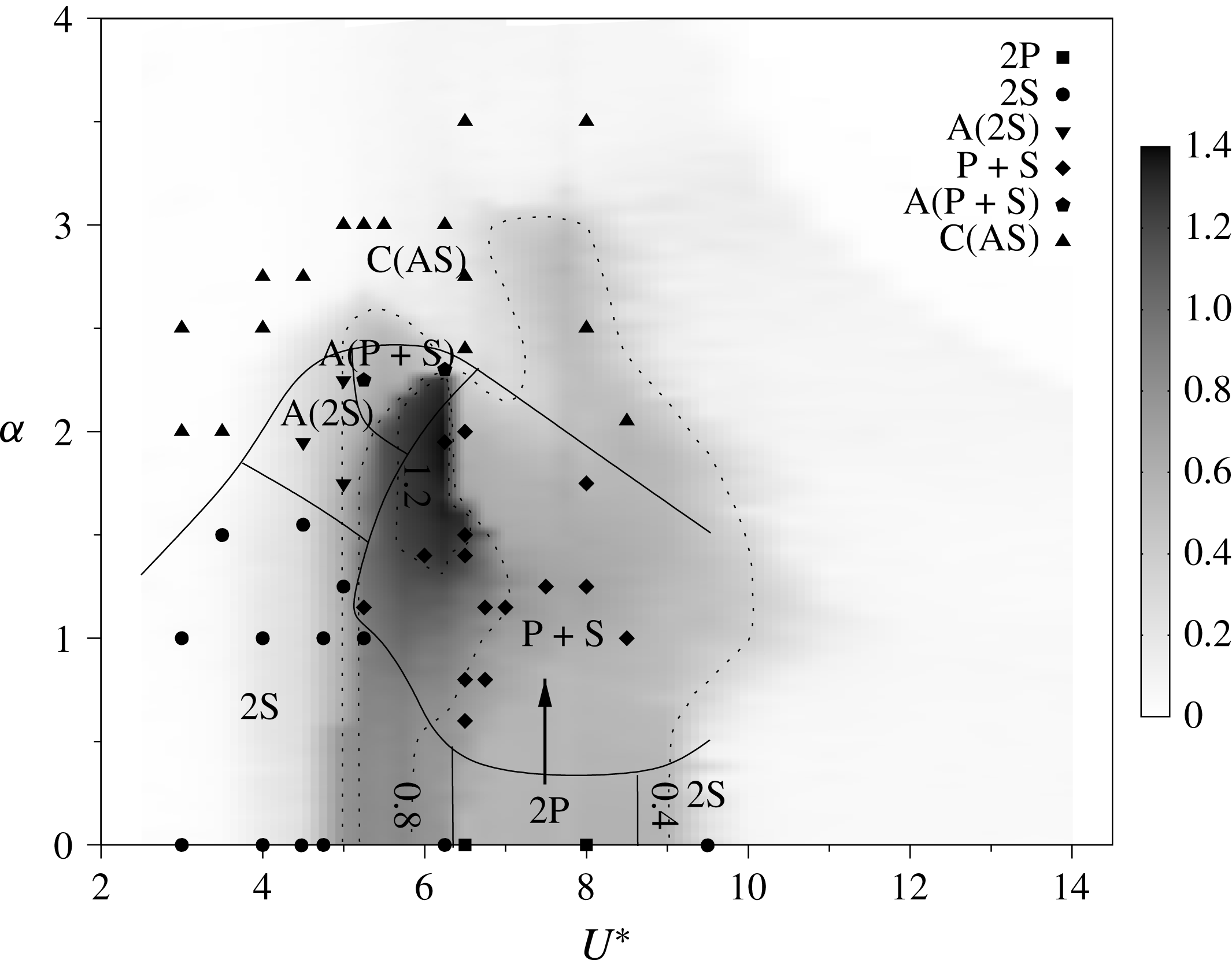
Figure 8 is a contour map of the mean response amplitude in
 $U^{\ast }$
–
 $\unicode[STIX]{x1D6FC}$
parameter space. The dashed lines are iso-amplitude contours. The wake patterns observed for selected PIV datasets (discussed in more detail below) are marked on this figure to indicate how the wake state affects the amplitude response. The solid lines represent approximate boundaries of regions with the same wake state. These are mainly drawn to aid in the interpretation of how the wake state and amplitude response are related.
Phase-averaged spanwise vorticity contours of a 2S mode at
 $U^{\ast }=5.0,~\unicode[STIX]{x1D6FC}=1.0$
(a), 2P mode at
 $U^{\ast }=8.0,~\unicode[STIX]{x1D6FC}=0.0$
(b) and
 $\text{P}+\text{S}$
mode at
 $U^{\ast }=6.5,~\unicode[STIX]{x1D6FC}=0.6$
(c) over an oscillation cycle. Cylinder rotation is anticlockwise. The normalised vorticity range is
 $\unicode[STIX]{x1D714}^{\ast }=\unicode[STIX]{x1D714}D/U\in [-1,1]$
, where
 $\unicode[STIX]{x1D714}$
is the vorticity. Near the cylinder the vorticity exceeds these values, so the contour levels are clipped to this range to allow downstream vortices to be visible.

As indicated above, a large number of PIV snapshots were gathered at a high sampling frequency capturing approximately 12–15 snapshots per cycle for typically 200–300 cycles (3140 images gathered). The recording of the PIV snapshots were synchronised with the cylinder motion.
To investigate the wake state beyond the PIV images, the classical snapshot method (Sirovich Reference Sirovich1987; Holmes et al.
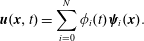
Reference Holmes, Lumley, Berkooz and Rowley2012) was followed using the MODRED 2.0.1 library to decompose the fields. The velocity field,
 $\boldsymbol{u}(\boldsymbol{x},t)$
, is decomposed as follows:
 $$\begin{eqnarray}\boldsymbol{u}(\boldsymbol{x},t)=\mathop{\sum }_{i=0}^{N}\unicode[STIX]{x1D719}_{i}(t)\unicode[STIX]{x1D74D}_{i}(\boldsymbol{x}).\end{eqnarray}$$
Here
 $\boldsymbol{x}$
is the illuminating laser plane coordinates,
 $N=3140$
is the number of snapshots taken,
 $\unicode[STIX]{x1D74D}(\boldsymbol{x})$
are the proper orthogonal decomposition (POD) spatial modes and
 $\unicode[STIX]{x1D719}(t)$
are the temporal mode coefficients. In the presence of periodic or near-periodic flow, the mean flow is approximately represented by
 $\unicode[STIX]{x1D74D}_{0}(\boldsymbol{x})$
, whereas, in terms of the shedding process, the first pair of temporal modes,
 $\unicode[STIX]{x1D719}_{1}$
and
 $\unicode[STIX]{x1D719}_{2}$
, together represent the most energetic shedding mode. The subsequent pair is often a harmonic of the first pair. Therefore, the first temporal coefficients (
 $\unicode[STIX]{x1D719}_{1}$
–
 $\unicode[STIX]{x1D719}_{4}$
) are often sufficient to assess the flow state and to reorder the velocity/vorticity fields into similar phases, as shown in Legrand et al. (Reference Legrand, Nogueira, Tachibana, Lecuona and Nauri2011), Sherry et al. (Reference Sherry, Nemes, Lo Jacono, Blackburn and Sheridan2013) and Venning et al. (Reference Venning, Lo Jacono, Burton, Thompson and Sheridan2015). All the PIV data were subsequently analysed with the POD approach and phase averaging was based on the temporal evolution of the first two modes associated with the main shedding behaviour. In the present study, the images in each set were categorised into 12 phases for averaging.
A non-rotating cylinder undergoing VIV shows hysteresis and wake mode switching in the transition regions between the amplitude response branches (Feng Reference Feng1968; Khalak & Williamson Reference Khalak and Williamson1999; Williamson & Govardhan Reference Williamson and Govardhan2004). A primary focus of the current study is to determine the wake patterns in
 $U^{\ast }$
–
 $\unicode[STIX]{x1D6FC}$
parameter space.
In low amplitude response regions, i.e. at reduced velocities associated with the initial response branch (
 $U^{\ast }<4.8$
) and in the desynchronised region (
 $U^{\ast }\geqslant 9.5$
), the shedding mode typically found for non-rotating VIV was observed up to a rotation rate of
 $\unicode[STIX]{x1D6FC}\approx 2.0$
. This wake is characterised by shedding two single counter-rotating vortices per oscillation cycle (figure 9). This is referred to as the 2S mode. This is the standard shedding mode commonly found in both stationary and non-rotating VIV studies.
Instantaneous isocontours of the C(AS) mode at
 $U^{\ast }=4.00,~\unicode[STIX]{x1D6FC}=2.75$
. The C(AS) wake pattern is of a chaotic nature and consists of small vortices patched around a curve. The normalised vorticity range is
 $\unicode[STIX]{x1D714}^{\ast }=\unicode[STIX]{x1D714}D/U\in [-1,1]$
.
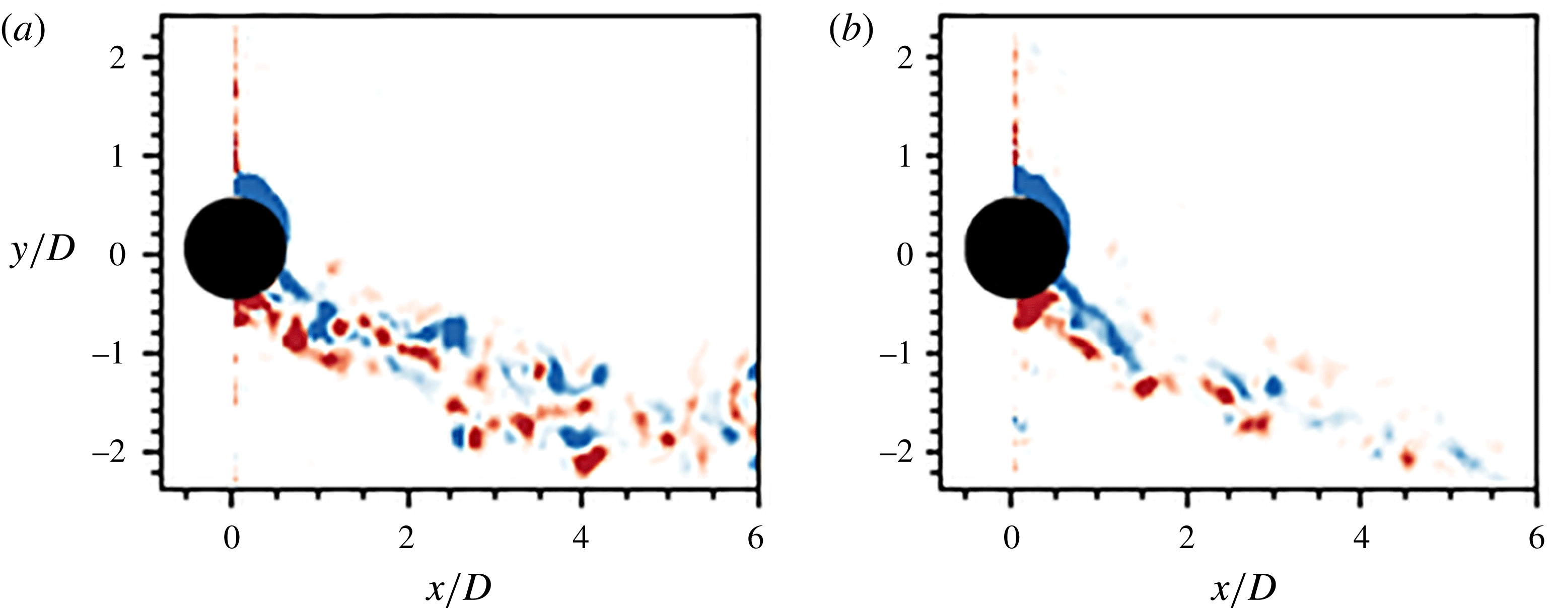
When the rotation rate is above
 $\unicode[STIX]{x1D6FC}\approx 2.0$
for the same reduced velocity ranges (
 $U^{\ast }<4.8$
,
 $U^{\ast }\geqslant 9.5$
), a new wake pattern characterised by shedding of small asymmetric vortices was observed. It appears similar to the shedding mode observed in the second region of wake instability reported by Mittal & Kumar (Reference Mittal and Kumar2003), although that mode was observed at significantly higher rotation rates (
 $\unicode[STIX]{x1D6FC}\sim 4.5$
). When the flow first undergoes transition to this mode, i.e. at its boundary with other wake modes, the vortices shed are larger and more periodic. As the rotation rate is increased further, the shed vortices become smaller and their shedding is more chaotic. However, it was observed that the wake switches between a wider and a narrower state, with the former associated with the shedding of smaller vortices. The coalescence of these small asymmetric vortices, together with its wake switching, has led to this mode to be named C(AS). Instantaneous spanwise vorticity contours for this mode are illustrated in figure 10: (b) illustrates the wider wake state; and (a) shows the narrower state.
At moderate reduced velocities associated with the lower amplitude response branch (
 $6.5\leqslant \unicode[STIX]{x1D6FC}\leqslant 9.5$
), where
 $0.4<A_{10}^{\ast }\leqslant 0.6$
and the rotation rate is below
 $\unicode[STIX]{x1D6FC}\leqslant 0.5$
, two pairs of counter-rotating vortices are shed per oscillation cycle (figure 9). This resembles the standard 2P mode reported in previous non-rotating VIV studies (e.g. Williamson & Roshko Reference Williamson and Roshko1988; Khalak & Williamson Reference Khalak and Williamson1999).
At moderate rotation rates (
 $1.25\leqslant \unicode[STIX]{x1D6FC}<2.25$
) a dominant wake mode persists across the vibration region (
 $5.0<U^{\ast }\leqslant 9.0$
), for which the wake and body motions synchronise. Here, the wake is characterised by the
 $\text{P}+\text{S}$
mode as shown in figure 9. This wake mode is composed of a pair (P) of counter-rotating vortices and a single (S) vortex shed per oscillation cycle. Again, this mode has been previously observed in free and forced vibration studies (see Williamson & Roshko Reference Williamson and Roshko1988). It has also been observed for the low-Reynolds-number rotating VIV simulations of BL14 and experiments of SM15.
Over the same reduced velocity range (
 $5.0<U^{\ast }\leqslant 9.0$
), the C(AS) wake mode appears when the rotation rate is increased above
 $\unicode[STIX]{x1D6FC}>2.25$
.
From figures 7 and 8, it is evident that large changes in the oscillation amplitude response correspond to changes in the wake mode. For example, in the case of
 $U^{\ast }=6.25$
, the drop in amplitude and jump in frequency response near
 $\unicode[STIX]{x1D6FC}=2.25$
coincide with a change in wake mode from 2S, in the unsteady flow regime, to the C(AS) mode, where the flow becomes almost steady. At the start of the lower branch (
 $U^{\ast }=6.5$
) there is a similar wake transition when
 $\text{P}+\text{S}$
undergoes transition to C(AS).
Phase-averaged spanwise vorticity contours of the 2S mode at different
 $\unicode[STIX]{x1D6FC}$
over an oscillation cycle:
 $U^{\ast }=5.00,~\unicode[STIX]{x1D6FC}=0.00$
(a–c),
 $U^{\ast }=5.00,~\unicode[STIX]{x1D6FC}=1.00$
(d–f) and
 $U^{\ast }=5.00,~\unicode[STIX]{x1D6FC}=2.25$
(g–i). Contours were selected to align the leading vortex of each oscillation cycle, i.e. the vortex with positive vorticity, to the trailing vortex of the previous oscillation cycle. This illustrates the effects of
 $\unicode[STIX]{x1D6FC}$
on wake asymmetry and the gap between vortices from adjacent oscillation cycles. Therefore, the contours between different
 $\unicode[STIX]{x1D6FC}$
are not necessarily in phase. The normalised vorticity range is
 $\unicode[STIX]{x1D714}^{\ast }=\unicode[STIX]{x1D714}D/U\in [-1,1]$
.
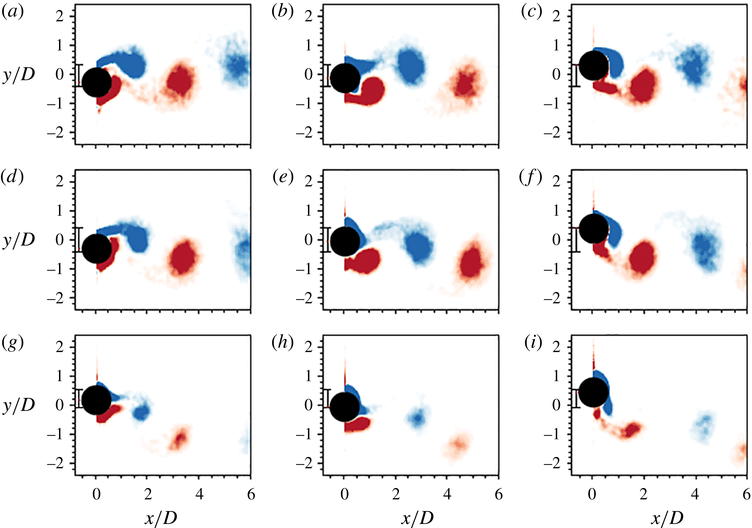
To further understand and characterise the effects of increasing rotation rate on the cylinder wake, the induced changes to the dominant 2S mode are examined. Figure 11 shows the progression of the 2S wake mode with increasing rotation rate at a constant reduced velocity of
 $U^{\ast }=5.0$
. In figure 11, (a–c) shows the characteristic vortex shedding for the non-rotating cylinder. Figure 11(d–f) and (g–i) show shedding at non-zero rotation rates:
 $\unicode[STIX]{x1D6FC}=1$
and
 $2.25$
, respectively. With increasing rotation rate, the mean position of the cylinder shifts upwards and the shed vortices deviate further downwards from the streamwise centreline as they advect downstream. This is expected as the body rotation causes wake deflection due to the Magnus effect.
Increased rotation also changes the spacing between the clockwise and anticlockwise vortex cores in the wake. With no rotation, the positive and negative vortex cores are distributed evenly along the wake. However, the addition of rotation means that the wake vortices show signs of collecting in pairs. This effect is enhanced with increasing rotation rate. This is shown in figure 11(c,f,i. It can be seen that, as the rotation rate is increased, the distance between a shed anticlockwise (red) vortex and the subsequently formed clockwise (blue) vortex is less than the distance between that vortex and the anticlockwise vortex shed next. With increasing rotation rate, the size and strength of shed vortices decreases. This has been seen in rotating cylinder wakes previously, e.g. figure 5 from Radi et al. (Reference Radi, Thompson, Rao, Hourigan and Sheridan2013). This is consistent with rotation causing the two separation points, which feed the shed vortices, to move together, thereby restricting the vorticity shed into each wake vortex and increasing cross-annihilation. Similar observations of the effects on the asymmetry and spacing are seen with the
 $\text{P}+\text{S}$
mode.
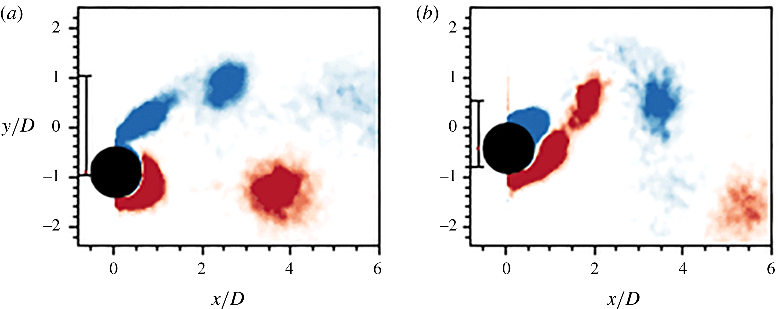
Images of the
 $\text{P}+\text{S}$
mode at different reduced velocities show a subtle change in the vortex pattern. Previous observations of the
 $\text{P}+\text{S}$
mode in VIV studies showed that it consisted of a single vortex on one side of the cylinder centreline, together with a clockwise and anticlockwise vortex pair on the other. Owing to symmetry in the non-rotating case, the pair and single vortices can form interchangeably on either side of the cylinder centreline. Figure 12 illustrates the
 $\text{P}+\text{S}$
mode in the upper amplitude response branch at
 $U^{\ast }=5.50$
(figure 12
a) and in the lower response branch at
 $U^{\ast }=6.5$
(figure 12
b). In the upper branch there are two clockwise vortices on the retreating side of the cylinder and one anticlockwise vortex on the advancing side of the cylinder. In the lower branch, the anticlockwise vortices on the advancing side of the cylinder that were previously observed in the upper branch remain. However, on the retreating side there are now one clockwise and one anticlockwise vortex. This observation was unexpected. It had been thought that the flow asymmetry created by the cylinder rotation would promote the shedding of vortices in one direction, hence the consistent combination of vortices seen in previous work (Williamson & Roshko Reference Williamson and Roshko1988; Morse & Williamson Reference Morse and Williamson2009) and figure 12(b). This result was observed at a range of rotation rates in the upper and lower branch. Further work is needed to better understand this behaviour.
Phase-averaged isocontours of the
 $\text{P}+\text{S}$
mode at
 $U^{\ast }=5.50,~\unicode[STIX]{x1D6FC}=1.15$
in the upper response branch (a) and
 $U^{\ast }=6.50,~\unicode[STIX]{x1D6FC}=0.60$
in the lower response branch (b). The normalised vorticity range is
 $\unicode[STIX]{x1D714}^{\ast }=\unicode[STIX]{x1D714}D/U\in [-1,1]$
.
3.3 Intermittent nature of the wake in the upper branch
When a cylinder undergoes VIV, previous studies have shown that, in the upper branch, the wake is of an intermittent or chaotic nature (Lucor & Triantafyllou Reference Lucor and Triantafyllou2008; Zhao et al. Reference Zhao, Leontini, Lo Jacono and Sheridan2014a ). One question of interest is whether this mode-switching signature of the upper branch still prevails when the cylinder is undergoing forced vibration. Indeed, the action of rotating fixed cylinders modifies the wake stability, whether the rotation is oscillatory (Tokumaru & Dimotakis Reference Tokumaru and Dimotakis1991; Lo Jacono et al. Reference Lo Jacono, Leontini, Thompson and Sheridan2010; D’Adamo, Godoy-Diana & Wesfreid Reference D’Adamo, Godoy-Diana and Wesfreid2015) or uniform (El Akoury et al. Reference El Akoury, Braza, Perrin, Harran and Hoarau2008; Rao et al. Reference Rao, Leontini, Thompson and Hourigan2013, Reference Rao, Radi, Leontini, Thompson, Sheridan and Hourigan2015). Thus, given that the cylinder is under uniform rotation, hence biasing the vorticity production towards one side and therefore biasing the wake topology, the question of how this affects the wake dynamics of the upper branch is of interest.
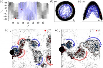
Instantaneous measurement showing transition from the 2P to 2S mode for
 $U^{\ast }=6.50$
and
 $\unicode[STIX]{x1D6FC}=0.0$
. (a) Time-varying body position
 $y^{\ast }=y^{\prime }/D$
, with
 $y^{\prime }=y-\bar{y}$
, as a function of
 $t^{\ast }=tf_{nw}$
. The black line represents the zone of 2P mode, and the blue line represents the zone of 2S mode. The red filled symbols (● and ▴) match the instantaneous vorticity fields presented in (d) and (e) showing a 2P and 2S mode, respectively, to the instantaneous positions in the other plots. Plots (b) and (c) represent the temporal evolution of the POD modes, highlighting the differences over time (i.e. providing different Lissajous shapes). See supplementary movie 1.

In the following, observations on the vortex wake state are presented for
 $U^{\ast }=6.5$
at three different rotation rates:
 $\unicode[STIX]{x1D6FC}=0.0,~0.8,~1.5$
. The switching of the wake state was identified from the inspection of the
 $\unicode[STIX]{x1D719}_{1}$
–
 $\unicode[STIX]{x1D719}_{4}$
POD temporal coefficients. The instantaneous amplitude provided by
 $y(t)$
was not enough to unambiguously decipher changes within the wake, as exemplified through figures 13–15. Given the substantial number of snapshots gathered (
 ${\sim}3100$
), covering a large number of shedding cycles (
 ${\sim}200$
–300), it is possible to observe many examples of mode switching. In the supplementary material associated with this paper (available at https://doi.org/10.1017/jfm.2017.540), movies displaying these transitions provide a useful adjunct to the still images presented in this section.
Figure 13 shows an example of this mode-switching behaviour for
 $\unicode[STIX]{x1D6FC}=0$
. This example shows the transition from a 2P to 2S shedding mode. The time history of the motion is given in figure 13(a), with the section in blue marking where mode switching is observed. The temporal evolution of the mode is represented through Lissajous figures of the first pair (
 $\unicode[STIX]{x1D719}_{1}$
and
 $\unicode[STIX]{x1D719}_{2}$
), and the first and third modes (
 $\unicode[STIX]{x1D719}_{1}$
and
 $\unicode[STIX]{x1D719}_{3}$
), in figure 13(b,c), respectively. The symbols (● and ▴) appearing in these plots in figure 13(a–c) correspond to the instantaneous vorticity fields given in figure 13(d,e), representing the 2P and 2S modes, respectively. Clearly, the information contained in the displacement signal
 $y(t)$
is not sufficient to reveal the behaviour within the wake, yet the changing form of the two Lissajous curves clearly differentiates the modes. In the supplementary movie, additional switching within the blue zone can be observed. Inspection of the POD temporal mode was instrumental to differentiate the wake dynamics and was only possible due to the large number of shedding periods recorded.
Instantaneous measurement showing transition from the
 $\text{P}+\text{S}^{+}$
to 2S shedding mode for
 $U^{\ast }=6.50$
and
 $\unicode[STIX]{x1D6FC}=0.80$
. (a) Time-varying body position
 $y^{\ast }$
as a function of
 $t^{\ast }$
. The black line represents the zone of
 $\text{P}+\text{S}^{+}$
mode, and the blue line represents the zone of 2S mode. The red filled symbols (● and ▴) correspond to the instantaneous vorticity presented in panels (d) and (e) showing a
 $\text{P}+\text{S}^{+}$
and 2S mode, respectively. Plots (b) and (c) are representative of the temporal POD mode evolution, highlighting the differences in time (providing different Lissajous shapes). See supplementary movie 2.

Figure 14 shows a further example of mode switching at
 $\unicode[STIX]{x1D6FC}=0.80$
. This example shows the transition from a
 $\text{P}+\text{S}^{+}$
to 2S shedding mode. Note that the S
 $^{+}$
represents an anticlockwise single vortex. The time history of the displacement trace is given in figure 14(a), with the mode switching zone coloured in blue. The temporal mode evolution is given through Lissajous figures of the first pair (
 $\unicode[STIX]{x1D719}_{1}$
and
 $\unicode[STIX]{x1D719}_{2}$
), and the first and third modes (
 $\unicode[STIX]{x1D719}_{1}$
and
 $\unicode[STIX]{x1D719}_{3}$
), in figure 14(b,c), respectively. The symbols appearing in figure 14(a–c) correspond to the instantaneous vorticity field given in figure 14(d,e), representing the
 $\text{P}+\text{S}^{+}$
and 2S modes, respectively. Again, the changing shape of the two Lissajous curves clearly differentiates the shedding modes, while the displacement signal
 $y(t)$
is not sufficient to reveal the mode switch.
As the rotation rate is increased to
 $\unicode[STIX]{x1D6FC}=1.50$
, the mode switching behaviour still prevails at
 $U^{\ast }=6.5$
. Figure 15 shows the transition from a
 $\text{P}+\text{S}^{-}$
to 2P mode. Note that S
 $^{-}$
represents a clockwise single vortex. As before, the time history of the motion is given, with the switch to blue marking the transition between wake states. Once again, the switch is clear through the change in the response depicted in the Lissajous figures (figure 15
b,c). The supplementary movie 3 further confirms these modes, noting that it can be difficult to interpret a shedding mode from a single instantaneous snapshot.
Instantaneous measurement showing transition from the
 $\text{P}+\text{S}^{-}$
to 2S shedding mode for
 $U^{\ast }=6.50$
and
 $\unicode[STIX]{x1D6FC}=1.50$
. (a) Time-varying body position
 $y^{\ast }$
as a function of
 $t^{\ast }$
. The black line represents the zone of
 $\text{P}+\text{S}^{-}$
mode, and the blue line represents the zone of 2S mode. The red filled symbols (● and ▴) correspond to the instantaneous vorticity presented in panels (d) and (e), showing a
 $\text{P}+\text{S}^{-}$
and 2P mode respectively. Plots (b) and (c) are representative of the temporal POD mode evolution, highlighting the differences in time (providing different Lissajous shapes). See supplementary movie 3.

It is acknowledged that the results presented do not provide a complete picture reflecting all possible transitions. However, the limited information reported is sufficient to confirm that the intermittent behaviour in the upper branch is sustained even for high rotation rates.
3.4 Discussion
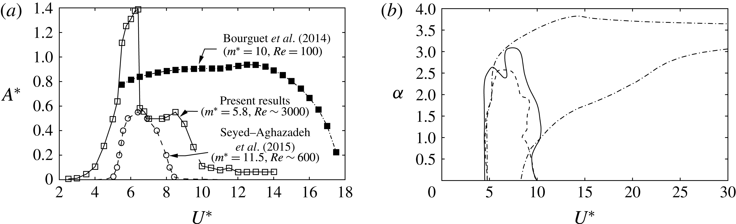
Figure 16(a) shows a comparison of the vibration response curve at
 $\unicode[STIX]{x1D6FC}=2$
with previous parameter studies from the literature. The response curve of SM15, who also performed experiments using a water channel for their VIV studies of a rotating cylinder, has been extracted from an amplitude contour plot in their paper. Their Reynolds-number range covers the interval
 $350\leqslant Re<1000$
, with the maximum response recorded for
 $U^{\ast }=6.5$
, corresponding to
 $Re\simeq 600$
. The
 $Re=100$
numerical results of BL14 are also shown for this rotation rate. The maximum response (
 $A^{\ast }\simeq 0.6D$
) found by SM15 actually occurred at a slightly higher rotation rate of
 $\unicode[STIX]{x1D6FC}\simeq 2.3$
, although this was only marginally in excess of the value recorded for the
 $\unicode[STIX]{x1D6FC}=2.0$
case shown. On the other hand, the low-Reynolds-number simulations of BL14 indicate that the vibration response continues to increase with rotation rate up to
 $\unicode[STIX]{x1D6FC}=4.0$
, after which there is minimal response. Notably, they also found a significant vibration response for a much larger
 $U^{\ast }$
range than observed in both sets of experiments. The different vibration response seen in the current experiments is likely to be due to the significantly higher Reynolds number (
 $Re=3000$
at
 $U^{\ast }=6.5$
) of the current study, rather than the different mass ratios (
 $m^{\ast }=5.78$
compared with
 $11.5$
and
 $10$
), or the different but low mass-damping ratios, of the different experiments and simulations. Figure 16(b) shows the approximate vibration response boundaries for these three cases, delimiting regions where the response is non-negligible. Interestingly, the two sets of experiments show similar boundaries, despite the distinct differences in amplitude response. The unstable region from the numerical simulations is also similar over the initial
 $U^{\ast }$
range for low
 $\unicode[STIX]{x1D6FC}$
but shows that significant vibration response extends up to high
 $U^{\ast }$
for larger values of
 $\unicode[STIX]{x1D6FC}$
.
(a) Comparison of the response curve for
 $\unicode[STIX]{x1D6FC}=2.0$
against previous numerical and experimental studies. Note, in particular, the much higher vibration response in this case. (b) Corresponding approximate vibration boundaries as a function of
 $U^{\ast }$
and
 $\unicode[STIX]{x1D6FC}$
. Refer to panel (a) for data references.
4 Conclusions
The present study on the vibration response and wake structure of an elastically mounted circular cylinder subjected to forced, constant rotation over a range of rotation rates and Reynolds numbers has made several new findings.
Substantial body vibration was found to occur through wake–body synchronisation over a range of rotation rates and reduced velocities. Significant cylinder oscillations were observed to occur for rotation rates up to
 $\unicode[STIX]{x1D6FC}\approx 3.5$
over the lock-in range. Interestingly, previous rigidly mounted cylinder studies show that rotation rates beyond
 $\unicode[STIX]{x1D6FC}=2$
cause suppression of vortex shedding. Overall, this study shows that forced rotation can cause the cylinder to vibrate at up to
 $1.4D$
, a
 $76\,\%$
increase in amplitude response over non-rotating VIV. This maximal response occurs when the rotation rate is close to
 $2.0$
and in the range of reduced velocities associated with the upper amplitude response branch of a non-rotating cylinder. Across the
 $U^{\ast }$
–
 $\unicode[STIX]{x1D6FC}$
parameter space where a large amplitude response is seen, the cylinder frequency response is observed to be synchronised with the natural frequency of the oscillating system. It is the resonance between these two frequencies that enables large vortex-induced oscillations for non-rotating VIV and also enables large oscillations for VIV of a rotating cylinder. Increasing the rotation rate from 0 to 2 both broadens the range of reduced velocities where large body oscillations occur and increases the peak amplitude response. As the rotation rate is increased towards
 $\unicode[STIX]{x1D6FC}\approx 2.0$
, the frequency response
 $f^{\ast }$
gradually decreases to fall below
 $f^{\ast }=1$
, where the oscillation frequency equals the natural frequency of the structure. This is correlated with the amplitude response increasing as the rotation rate is increased towards
 $\unicode[STIX]{x1D6FC}\approx 2.0$
. An increase in rotation rate beyond
 $\unicode[STIX]{x1D6FC}\approx 2.0$
results in a reduced peak amplitude response, noting that the body oscillation becomes desynchronised with the weakened, less coherent vortex shedding.
A variety of wake modes were observed over the parameter space covered by the present study. At low to moderate reduced velocities (
 $U^{\ast }<6.5$
), the 2S mode dominates at all rotation rates observed. At low rotation rates (
 $\unicode[STIX]{x1D6FC}<1.25$
), the 2S and 2P modes characterise the wake at reduced velocities associated with the upper and lower response branches, respectively. In the desynchronised region, the 2S mode appears again. At moderate rotation rates (
 $1.25\leqslant \unicode[STIX]{x1D6FC}<2.25$
), the
 $\text{P}+\text{S}$
mode, a mode composed of a pair of counter-rotating vortices and a single vortex shed per cycle, was observed for most of the synchronisation region. Chaotic switching of the wake mode was observed in the upper branch. Indeed, it was found that, regardless of the rotation rate, the upper response branch seemed to retain its chaotic state. In the desynchronised region, a mode in which small-scale vortices coalesce and shed asymmetrically, C(AS), was observed at rotation rates above
 $\unicode[STIX]{x1D6FC}\approx 1.25$
. Beyond
 $\unicode[STIX]{x1D6FC}\approx 2.25$
, C(AS) dominates in the reduced velocity range associated with the vibration region of a non-rotating cylinder (
 $U^{\ast }\approx 4{-}10$
). On further increasing the rotation rate, shed vortices increasingly deviate from the streamwise centreline of the cylinder. This deviation with rotation rate was observed for multiple wake modes, as is expected from the Magnus effect. In addition, the distance between vortices of adjacent oscillation cycles increases, and the size and peak vorticity of the vortices shed decreases, in line with non-VIV studies.
Of further interest is the significantly lower amplitude response observed experimentally by Seyed-Aghazadeh & Modarres-Sadeghi (Reference Seyed-Aghazadeh and Modarres-Sadeghi2015) relative to that found in this case. Given the substantial Reynolds-number difference between these studies, this could simply be a low-Reynolds-number effect, but it would be useful to have independent verification of either study. In a sense, it is surprising that rotation significantly enhances vibration amplitudes, given that it tends to make the wake narrower and asymmetric, so a deeper understanding of the near-wake dynamics and the effects on VIV would be useful. Also of interest is the still significant amplitude response observed at
 $\unicode[STIX]{x1D6FC}=2.5$
and
 $3$
, well beyond the rotation rate for suppressing shedding from a fixed rotating cylinder, which warrants further investigation.
Acknowledgements
The authors acknowledge financial support from Australian Research Council Discovery Project grants DP110102141 and DP150102879. The authors would like to acknowledge the financial support of the Centre National de la Recherche Scientifique (CNRS) through grant no. PICS161793 under the Projet International de Coopération Scientifique. K.W.L. acknowledges financial support from a Commonwealth sponsored Australian Postgraduate Award (APA) for his PhD study.
Supplementary movies
Supplementary movies are available at https://doi.org/10.1017/jfm.2017.540.