1. INTRODUCTION
The detection of a unit root in the characteristic polynomial of an autoregressive model is still one of the most debated issues in time series analysis (see, e.g., Phillips and Xiao, 1998). This is a big issue concerned with distinguishing stationary time series from time series for which differencing is required to induce stationarity, and in practice it is usually addressed through formal hypothesis testing.
In recent years, however, there has been more and more interest in the Bayesian approach to this problem, leading to the comparison of stationary models with those involving a unit autoregressive root via the calculation of posterior odds and of Bayes factors (for a different model selection criterion based on predictive densities see Phillips and Ploberger, 1994).
In particular, the literature has devoted great attention to the nature of suitable noninformative priors for the autoregressive coefficients. As a few examples consider the work of Sims (1988) and Sims and Uhlig (1991), who advocate the use of flat priors. Phillips (1991a) finds that flat priors bias the inference toward stationary models and suggests instead using Jeffreys priors derived from conditional likelihood functions. Also Uhlig (1994a) determines the Jeffreys priors for an AR(1) process from the exact likelihoods and justifies the use of flat priors only in some specific cases. Uhlig (1994b) summarizes most of the Bayesian contribution to the unit root problem and discusses the sensitivity of the tails of the predictive densities on the prior treatment of explosive roots. Schotman and Van Dijk (1991a) stress the sensitivity of the posterior odds to the size of the stationary region and suggest restricting this size. Many authors (e.g., Schotman and Van Dijk, 1991b; Phillips, 1991b; Zivot, 1994; Marriott and Newbold, 1998) note that, in the unit root case, the lack of identifiability of the process level parameter implies that any improper prior on this parameter generates a posterior probability for the unit root hypothesis that goes to one. Berger and Yang (1994) consider a reference prior approach for the AR(1) model. Marinucci and Petrella (1999) also derive a noninformative prior for the AR(1) model by considering the functional relationship between the autoregressive parameter and the variance of the process. It is particularly interesting to note the paper by Marriott and Newbold (1998), who criticize the use of priors such as the uniform or the Jeffreys prior for the autoregressive coefficients in this setting and advocate the use of sharp, informative prior distributions. However, for the simple problem of testing for a unit root in a first-order autoregressive process, they find that the prior distribution for the autoregressive coefficient has a substantial impact on the posterior odds, so that, e.g., a very sharp beta prior performs extremely well when the generating process is stationary autoregressive, but the uniform prior is preferable when the “true” model is nonstationary. To better clarify this point, consider the two models Yt = Yt−1 + ηt versus Yt = φ1Yt−1 + ηt where {ηt} is a Gaussian white noise process and assume a flat prior for φ1. If the data are nearly a random walk then the standard procedure is heavily tilted toward finding a unit root, because a flat prior over φ1 assigns a lot of a priori probability to parameters that we know from the start will have little chance at explaining the data.
The purpose of the present paper is to further investigate the choice of the prior distribution for the autoregressive coefficients in this setting and to derive a procedure for the identification of the order of an autoregressive model for an observed time series and the detection of a unit root in its characteristic polynomial, which is robust with respect to such prior. To make the model comparison robust to the choice of priors for the autoregressive coefficients, one could use the first l observations for training and let the rest of the data choose a model. In the preceding example, e.g., the updated prior for φ1 already will be concentrated on the values that are more plausible for explaining the data. Here, to avoid the choice of a specific training sample, we suggest using updated versions of the priors obtained from suitable training likelihoods based on all observations. As in Marriott and Newbold (1998) we remove the problem of the lack of identifiability of the level parameter by considering the first differences of the original series. Furthermore, as the alternative hypothesis to the stationary case, we consider the unit root model, assigning null prior probability to explosive roots (for a discussion on the unit root as hypothesis of interest, see Schotman and Van Dijk, 1991b). Also, we introduce a new parametrization to allow expressing the prior distributions on the parameters of the models under comparison through conditional distributions obtained from the prior assigned to the largest model.
The models and notation are introduced in Section 2, and the general ideas and key tools for comparing different models in the Bayesian setting are introduced in Section 3; particular attention is devoted to model selection problems for dependent data with weak prior information and to alternative Bayes factors. The marginal distributions for computing the Bayes factors and posterior odds are derived in Section 4. Section 5 considers in detail the simple problem of testing for a unit root in a first-order autoregressive process, and Section 6 deals with the more general case in which the order of the process is also unknown. A few concluding remarks are presented in Section 7.
2. MODELS AND NOTATION
Let

be a Gaussian stationary stochastic process with mean

. The process {Yt} is said to be an autoregressive process of order p (ARMA(p,0)) if it may be represented as

where φp(B) = 1 − φ1 B − ··· − φp Bp is the autoregressive polynomial, B is the backshift operator such that BkYt = Yt−k, and {ηt} is a Gaussian white noise process with variance τ2; the stationarity condition constrains the parameter vector φ(p) = (φ1,φ2,…, φp) to lie in the stationarity region {φ(p) : φp(z) = 0 implies |z| > 1}.
Suppose we observe the time series y = (y1,…, yn), a finite realization of an autoregressive process of order p, with p unknown; the goal is the identification of p and the simultaneous test for a unit root in the autoregressive polynomial.
Recall that if in the generating process there is a unit autoregressive root, stationarity can be achieved by considering the first differences of the original series. In fact in this case, letting Zt = Yt+1 − Yt, the process {Zt} is stationary ARMA(p − 1,0) and can be represented as

where φp−1(B) = 1 − φ1 B − ··· − φp−1 Bp−1 and

.
It follows that for fixed p, the test for a unit root can be performed by choosing between (1) and (2). However, the use of Bayes factors requires that the comparison between models is done by considering the same observations; thus, following Marriott and Newbold (1998), we also write the stationary process (1) in terms of the first differences. In particular, it is straightforward to verify that if {Yt} is stationary ARMA(p,0), the process {Zt} is stationary ARMA(p,1) with moving average coefficient equal to 1 and can be represented in terms of the parameter vector φ(p) as

or equivalently in terms of φ(p−1) = (φ1,φ2,…, φp−1) and φ0 as

where φ0 = φ1 if p = 1 and

otherwise, and

This latter representation has the advantage of emphasizing that the ARMA(p − 1,0) model (2) is nested in the ARMA(p,1) model (4) and can be obtained from (4) by letting φ0 = 1. More generally, the smaller models ARMA(p − h,0),h = 2,…, p, and ARMA(p − h,1),h = 1,…, p − 1, can be obtained from (4) simply by letting φp−1 = ··· = φp−h+1 = 0, φ0 = 1 and φp−1 = ··· = φp−h = 0, respectively.
Now for a given order p, the test for a unit root can be performed by comparing model (4) and model (2) for the first differences zt = yt+1 − yt (t = 1,…, n − 1); if p is also unknown, the problem of identifying the model for an observed time series and testing for a unit root can be seen as the one of choosing a model for the first differences in the set

where

is a set of possible values for p and Mp,q denote the stationary ARMA(p,q) model for z = (z1,…, zn−1)

.
It should be noted that the primary motivation in Marriott and Newbold (1998) for conducting the analysis in first differences is that this allows them to circumvent having to specify a prior distribution for the mean μ. In fact, Marriott and Newbold (1998) argued that under the stationary model a reasonable prior for μ is the (improper) uniform prior. However, because μ is unidentified under the unit root model, specification of an improper uniform prior will result in an indeterminacy in the Bayes factor. Hence, doing the analysis in the first differences allows them to get around this problem. In the following section we discuss more generally the issue of the sensitivity of the Bayes factor to prior assumptions, and we review some methods recently proposed in the literature for dealing with this problem.
3. BAYES FACTORS AND ALTERNATIVE BAYES FACTORS
The choice of the model that better fits the data is a crucial problem in the various approaches to statistical inference; in the Bayesian setting the key tool for model comparison is the Bayes factor.
Suppose we are comparing two models, Mi and Mj, and let fr(z|θr) and πr(θr) be, respectively, the distribution of the data and the prior distribution of the parameters θr under model Mr (r = i,j). The Bayes factor for Mi against Mj is defined as

and it represents the weight of evidence in the data in favor of Mi against Mj. Combining this information with the prior odds we then obtain the posterior probabilities of the models under comparison. Then, e.g., we can predict future observations by taking a weighted average of the optimal predictors for each model, with weights given by these posterior probabilities.
Many problems arise, however, when using the Bayes factor if the prior information is weak, mainly as a consequence of its sensitivity to prior assumptions. In fact, when the prior distributions are proper but diffuse, the more flat the prior, the more penalized the corresponding model; moreover, when they are improper, i.e., defined only up to arbitrary constants, then the Bayes factor is itself a multiple of these constants.
Thus, when the prior information is weak, various authors suggest the use of partial Bayes factors: the idea is to use part of the data as a training sample to update the prior distributions and the remainder of the data to compare the models. Formally, divide the data into two parts. First, subsample z(l) of size l is used to obtain the posterior distributions πr(θr|z(l)); in the second step, taking these as prior distributions, the remaining data z(−l) are used to compute a Bayes factor:

As discussed in O'Hagan (1995, 1997) and in De Santis and Spezzaferri (1997, 1999), partial Bayes factors are less sensitive to prior distributions than Bayes factors. In fact, if z(l) is a proper training sample, i.e., is such that the updated prior distributions πr(θr|z(l)) are proper for r = i,j, partial Bayes factors do not depend on arbitrary constants when improper priors are used. Furthermore, they are well defined also with proper priors, and they have the appealing property of balancing the bias introduced to Bayes factors by flat (proper) priors; it follows that they can be successfully used not only as automatic methods when the prior distributions are improper but also in the robust approach to model selection.
There is, however, a difficulty with the use of partial Bayes factors, namely, the selection of the training sample from the data. Among the different proposals to remove the dependence of the partial Bayes factor on a specific training sample, it is particularly interesting to look at that of De Santis and Spezzaferri (1997, 2001), who suggested replacing the likelihood fr(z(l)|θr) in (6) with the geometric training likelihood frl(z|θr), defined as the geometric mean of the fr(z(l)|θr) as z(l) varies over the set of all possible proper training samples of a given size l (r = i,j). For independent and identically distributed (i.i.d.) data this proposal leads to the fractional Bayes factor (O'Hagan, 1991, 1995), but in more general situations, where the use of fractional Bayes factor is not justified as it is in the case of dependent data, the geometric training likelihood can be used to introduce a new tool for Bayesian model choice with weak prior information, which we can refer to as the generalized fractional Bayes factor.
Now, when choosing a model in (5), because of the stationarity constraints, the choice of the prior distribution for the autoregressive parameters under both the stationary model and the integrated one does not represent a problem for the evaluation of Bayes factors and of posterior odds; in fact, even if we assume noninformative priors for these parameters, on the stationarity regions these turn out to be proper. On the other hand, if the prior distribution for τ2 is improper, the Bayes factor for comparing any two models in (5) is undefined. Now, it may be argued that because τ2 appears in all the models in (5), the (unknown) multiplicative constants in the Bayes factor would cancel; however, as pointed out in Berger and Pericchi (1996), this is a dangerous practice because what appears to be the same parameter can have very different interpretations, and therefore different prior distributions, under different models. Moreover, whether or not the prior for τ2 is improper, it was shown by Marriott and Newbold (1998) that the standard Bayesian analysis is extremely nonrobust with respect to the choice of the prior distribution for the autoregressive coefficients. Thus, we will adopt a robust approach and in particular focus our attention on the generalized fractional Bayes factor.
One last issue is worth some consideration. The choice of the size of the training sample has been widely discussed in the literature; see, e.g., O'Hagan (1995, 1997). One simple and obvious choice that has proved to be reliable in a range of problems involving improper priors is to consider the minimal training sample, i.e., the smallest sample size needed to update an improper prior so as to obtain a proper prior distribution. On the other hand, it is interesting to note the paper by Conigliani and O'Hagan (2000); through the analysis of a suitable sensitivity measure the authors prove that, within the fractional Bayes factor approach, greater robustness with respect to misspecification of the priors can be achieved by increasing the size of the training sample. Here, if we consider an improper prior for τ2, a minimal training sample is any subset of z made of a single observation zt (t = 1,2,…, n − 1). Being a proper training sample, each zt carries enough information to update the prior distribution for τ2 and turn it into a proper distribution. On the other hand, being minimal, it does not carry any other information, and in particular it does not carry any information about the autoregressive coefficients; in this sense, to learn also about the autoregressive coefficients and to reduce the impact of their prior distribution on posterior odds and Bayes factors, we expect larger training samples to be more appropriate.
4. COMPUTING THE GENERALIZED FRACTIONAL BAYES FACTOR
Suppose we intend to select a model in (5) for a set of observations z = (z1,…, zn−1). Let fp,q(z|·) be the distribution of the data, θp,q be the vector of parameters, and πp,q(θp,q) be the prior distribution of the parameters under each model Mp,q in (5)

; clearly, from Section 2, and letting φ0(p) = (φ0,φ1,…, φp−1),

and

Moreover, let z(l) be a training sample of size l and let fp,ql(z|θp,q) be the geometric training likelihood of size l under Mp,q. The generalized fractional Bayes factor for comparing any two models in (5), say, Mi,δ and Mj,γ, is defined as

where

and

are the marginal distributions under Mp,q corresponding to the full likelihood, and to the geometric training likelihood, respectively (p = i,j;q = δ,γ).
We now determine the various marginal distributions needed for comparing all models in (5). First, note that because of the stationarity constraints, under both Mp,1 and Mp,0 we can define the exact likelihood function (Box, Jenkins, and Reinsel, 1994). Moreover, note that as the integrals with respect to the autoregressive coefficients, assuming either informative or noninformative priors for these parameters, cannot be solved analytically, here we do not specify a particular form for πp,1(φ0(p)) and πp,0(φ(p)), whereas for τ2 we assumed the standard noninformative prior


. However, there is one issue concerning the priors πp,1 and πp,0 that is worth emphasizing. Let p be the maximum value of p in the set

defined in (5) and consider a prior πp,1(φ0(p)) assigned on the stationary region of the largest model Mp,1 in (5). As previously noted all the other models Mp−h,1 and Mp−h,0(h = 1,…, p − 1) in (5) can be obtained from Mp,1. It follows that extending πp,1 by continuity on the set φ0 = 1, as priors for the parameters φ0(p−h) and φ(p−h) under models Mp−h,1 and Mp−h,0 we can consider the conditional distributions

and

respectively. It is shown in the Appendix that the preceding distributions are defined on the stationary regions of the corresponding models.
Finally note that when we let l = 1, i.e., the size of the minimal training sample, for all p and for all q the marginal distribution corresponding to the geometric training likelihood under Mp,q is

i.e., is independent of p and q, and also of the prior distribution for the autoregressive parameters φ(p) and φ0(p). This is an important point: it confirms that minimal training samples do not carry enough information about the autoregressive parameters; moreover, it implies that when l = 1, the generalized fractional Bayes factor for comparing any two models in (5) equals the corresponding standard Bayes factor. For this reason, to achieve robustness with respect to the choice of the prior distributions for the autoregressive coefficients, we consider the case l > 1. In particular, as it was noted in Varshavsky (1996) and Barbieri and Conigliani (1998, 2000) that in the time series setup it seems natural to preserve the time structure for the training samples, instead of considering all possible subsets of the data of a given size, when computing the geometric training likelihood we consider only subsamples zk(l) = (zk+1,…, zk+l) made of successive observations.
Consider Mp,0 first and suppose that p > 0. Let τ2Vp−1 be the variance and covariance matrix of p consecutive variables of the stationary process (2) and let vts be the (t,s) element of Vp; following Galbraith and Galbraith (1974)

and

and the other elements of the matrix may be determined by noting that Vp is symmetric with respect to both its principal diagonals. Then the marginal distributions corresponding to the full likelihood and to the geometric training likelihood can be written as

and, for l > p,

respectively, where

Instead, if p = 0, z = (z1,…, zn−1) is a realization of a white noise process, so that

and

Now consider model Mp,1 and suppose that p > 0. Let τ2Wp−1 be the variance and covariance matrix of p consecutive variables of the process (4), b = (0,…,0,1) be a vector with p − 1 elements equal to 0 and the last element equal to 1, and D be the block matrix defined by

Then, following Galbraith and Galbraith (1974), the marginal distributions corresponding to the full likelihood and to the geometric training likelihood can be written as

and, for l > p,

respectively, where rts is the (t,s) element of the (n − 1) × (n − 1) matrix R defined by R = A′A − (H′A)′(D + H′H)−1(H′A), A is a lower triangular (n − 1) × (n − 1) matrix with (r,s) element ars given by

H is the (n − 1) × (p + 1) matrix with (i,j) element hij given by

(where we use the convention that for all j = 1,…, p, hij = 0 if i < 1),

is the (t,s) element of the l × l matrix

defined by

,

is the lower triangular l × l matrix obtained from A by considering the first l elements of the first l rows of A, and

is the l × (p + 1) matrix with rows given by the first l rows of H.
5. TESTING FOR A UNIT ROOT IN A FIRST-ORDER AUTOREGRESSIVE PROCESS: A SIMULATION EXPERIMENT
Let y = (y1,…, yn) be a finite realization of a first-order autoregressive process. As discussed in Section 2, the problem of testing for a unit root in its characteristic polynomial can be solved with reference to the differenced time series z = (z1,…, zn−1) by comparing the ARMA(1,1) model M1,1

and the ARMA(0,0) model M0,0

As pointed out in the Introduction, this problem was considered in detail in Marriott and Newbold (1998), with particular attention devoted to the problem of the sensitivity of the standard Bayesian analysis with respect to the choice of the prior distribution for the autoregressive coefficient. In fact, they criticize the use of priors such as the uniform or the Jeffreys prior for the autoregressive coefficient in this setting, the argument being that it is unreasonable to hold such vague prior belief while at the same time attaching nonzero probability mass at φ0 = 1. Instead, they advocate the use of sharp, informative prior distributions, with densities giving more prior weight to values of φ0 close to one; in particular, they find that a realistic representation of the beliefs of an investigator considering the random walk model as a possible explanation for the behavior of a series is a beta distribution with parameters (α = 5,β = 0.5) or (α = 50,β = 0.5), the latter being a sharper distribution with mean and variance approximately equal to 0.98 and 0.0008.
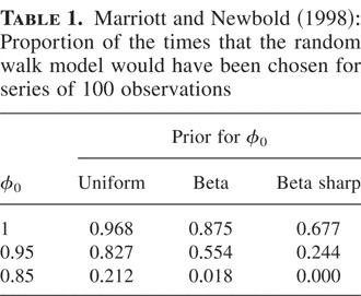
Thus, they generated 1,000 samples of 100 observations from first-order autoregressive processes with different values of φ0, and for each sample they computed the Bayes factor B(1,1)(0,0)(z) considering either the uniform prior, the beta prior, or the sharp beta prior for φ0. Assuming equal prior probabilities for the two models they computed the proportion of the samples for which the posterior probability of M0,0, i.e.,

is greater than ½. The results are presented in Table 1 and led the authors to conclude that the sharp beta prior performed extremely well when the “true” process was stationary autoregressive, whereas the opposite was the case for a random walk generating process, in which case the uniform prior should be preferred. The authors conclude that the choice of the prior distribution for φ0 is particularly relevant, so that special care should be devoted to elicit such a prior and “automatic” choices of noninformative priors such as the uniform should be avoided.
Marriott and Newbold (1998): Proportion of the times that the random walk model would have been chosen for series of 100 observations

For purposes of comparison we consider here the same model selection problem and solve it by means of the generalized fractional Bayes factor B(1,1)(0,0)l(z). We also explore the behavior of a triangular prior of the form

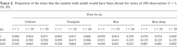
which is somehow intermediate between the uniform and the beta. The results are presented in Table 2, and we will see that they lead to very different conclusions with respect to those in Marriott and Newbold (1998), in favor of the use of noninformative priors.
Proportion of the times that the random walk model would have been chosen for series of 100 observations (l = 1, 10, 20)

Two issues clearly arise from Table 2, as a direct consequence of the use of the updated priors in the generalized fractional Bayes factor (7). First, notice that as l increases, the differences in the behavior of the various prior distributions are less relevant. In fact, whereas for l = 1 we obtain results in accordance with those in Marriott and Newbold (1998), when l = 20 the uniform prior, the triangular prior, and the beta prior give similar results both when the “true” process is stationary autoregressive and when it is a random walk. Second, as l increases the uniform prior performs better than when l = 1 in the stationary case and only slightly worse in the random walk case. Similar behavior is shared also by the triangular and beta prior, whereas no improvements are obtained by increasing l when using the beta sharp.
Indeed, the sharper the prior, the less the updated prior distribution is sensitive to the training likelihood, so that we did not expect the behavior of the beta sharp to change significantly by increasing l. Moreover, it is not surprising that if in the stationary case we assume a prior distribution that gives a lot of prior weight in the neighborhood of the true φ0, this will always perform better than a flat prior, no matter what the value of l. And in fact for l = 20 the uniform prior still (wrongly) favors the unit root model more often than the beta sharp for both φ0 = 0.95 and φ0 = 0.85.
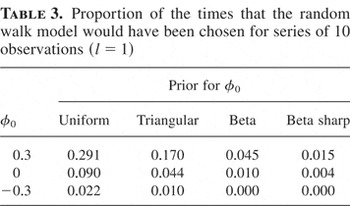
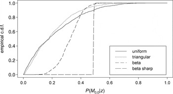
To further investigate this issue, we compare the performance of the different priors simulating series of 10 observations from first-order autoregressive processes with φ0 = 0.3, 0, −0.3; note that with samples of 100 observations, whatever prior we assume for φ0, the random walk model would never be chosen in these cases. The results are presented in Table 3 for l = 1 and again show that the two beta priors perform slightly better than the uniform and the triangular prior when the true process is stationary. However, it is interesting to look also at the shapes of the empirical cumulative distribution function for the posterior probability of M0,0. For instance if we consider the case φ0 = 0, we can see from Figure 1 that under either one of the beta priors the empirical c.d.f.s for P(M0,0|z) exhibit a steep growth around the median, so that only very rarely will P(M0,0|z) be either very large or very small. In other words, although the posterior probabilities corresponding to the beta priors almost always choose the right model, they hardly ever provide strong evidence in favor of the stationary model as the uniform prior does. The behavior of the four c.d.f.s in Figure 1 can also be synthesized by averages and standard deviations of the simulated values of P(M0,0|z). They are, respectively, 0.21858 and 0.17975 under the uniform prior, 0.19879 and 0.14547 under the triangular prior, 0.32313 and 0.07920 under the beta prior, and 0.48758 and 0.00251 under the beta sharp.
Proportion of the times that the random walk model would have been chosen for series of 10 observations (l = 1)


Empirical c.d.f. for P(M0,0|z) for series of 10 observations (l = 1,φ0 = 0).
These results are particularly interesting and suggest that even in the stationary case very sharp prior distributions perform rather poorly. In fact, for almost all samples generated from the stationary model, under the beta sharp the posterior odds are practically equal to the prior odds, and the information on the true model contained in the data is ignored. The same problem in terms of posterior uncertainty in the model choice can be observed also in the simulation experiment summarized in Table 2. Really, when we use the beta sharp we effectively compare models that are very close to each other and practically indistinguishable. For this reason we argue that the criterion based on the proportion of the samples for which the posterior probability of one model is greater than ½ can be misleading when comparing the different priors. A better understanding of the implications on the posterior odds of the prior specification can be achieved by looking at the shape of the empirical cumulative distribution functions. Moreover, we argue that a more disperse distribution such as the uniform, together with an appropriate size l of the training samples, should be preferred.
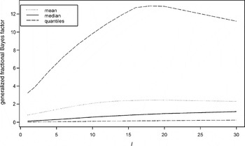
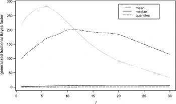
As for the problem of what an appropriate size of the training samples could be, some useful indications can be obtained from Figures 2 and 3, which show how the distribution of the generalized fractional Bayes factor varies with l when we assume a uniform prior for φ0. In particular, for the simulation experiment of Table 2, the two figures show the mean, the median, and the 2.5% and the 97.5% quantiles of B(1,1)(0,0)l(z) for φ0 = 0.95 and φ0 = 0.85, respectively. In both cases we see that at l = 1 the distribution of the generalized fractional Bayes factor is significantly concentrated on the interval (0,1). Then, as l starts to increase, it gives more weight to values bigger than 1, so that less often B(1,1)(0,0)l(z) wrongly chooses the random walk model. Finally, for large values of l, the mass of the distribution tends to be concentrated on 1, because the more observations are used for training, the fewer observations are left to choose between the models; in the limiting case, as l approaches n = 100, no model choice can be done.

Summaries of the distribution of the generalized fractional Bayes factor for different values of l (φ0 = 0.95).

Summaries of the distribution of the generalized fractional Bayes factor for different values of l (φ0 = 0.85).
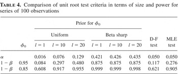
Finally, note that although our approach is fully Bayesian, its performance also can be interpreted within the usual hypothesis testing framework. Table 4 shows some of the results of Table 2 in terms of size and power of the test, together with those derived in Pantula, Gonzales-Farias, and Fuller (1994) concerning the usual Dickey–Fuller (D-F) test and a test based on maximum likelihood estimation (MLE). Note that in the uniform case considerably more power can be achieved by increasing l, whereas the size of the test increases only slightly.
Comparison of unit root test criteria in terms of size and power for series of 100 observations

6. TESTING FOR A UNIT ROOT AND ESTIMATING THE ORDER OF AN AUTOREGRESSIVE PROCESS: A SIMULATION EXPERIMENT
Let y = (y1,…, yn) be a finite realization of an autoregressive process of order p unknown and suppose that p varies in the set

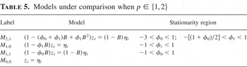
. As discussed in Section 2, the problem of identifying the model for this series can be solved with reference to the differenced time series z = (z1,…, zn−1) by comparing the models summarized in Table 5.
Models under comparison when p ∈ {1,2}

For the specification of the prior distributions under these models, two points should be taken into account. First, note that all models are nested in M2,1; in particular, M1,0, M1,1, and M0,0 can be obtained from M2,1 by letting φ0 = 1, φ1 = 0, and (φ0,φ1) = (1,0), respectively. It follows that once π2,1(φ0,φ1) is introduced under M2,1, the priors to be considered under M1,0 and M1,1 are the conditional distributions:

and

respectively (extending π2,1 by continuity on the set {φ0 = 1}). Moreover, if π2,1(φ0,φ1) is defined on the stationarity region of M2,1, then the preceding conditional distributions are defined on the stationarity regions of the corresponding models (see the Appendix).
Second, to express explicitly the prior belief on the presence of a unit root, under M2,1 we specify π2,1(φ0,φ1) by introducing a prior distribution for φ0, π2,1(φ0), and a prior distribution for the remaining parameter conditionally on φ0, π2,1(φ1|φ0); by doing so, we can compare the performance of the different prior distributions for φ0 considered in the previous section. In particular, we assume π2,1(φ1|φ0) to be uniform on the interval (−[(1 + φ0)/2];1) and π2,1(φ0) to be either uniform, beta, or beta sharp on (−3;1); the corresponding prior distributions under the remaining models are a uniform distribution on (−1;1) for φ1 under M1,0, and either a uniform, a beta, or a beta sharp on (−1;1) for φ0 under M1,1.
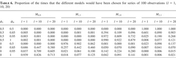
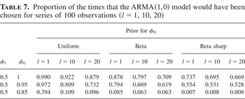
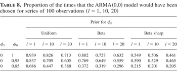
The results, corresponding to different sizes l of the training samples, are presented in Tables 6, 7, and 8. In particular, assuming a uniform prior for φ0, Table 6 illustrates the performance of our procedure with emphasis on the identification of the order of the autoregressive process; as expected, for all p the uncertainty between the stationary model that generated the data and the corresponding integrated one increases as φ0 approaches 1. The results in Tables 7 and 8 emphasize the effects of the different prior distributions for φ0 on the performance of the proposed method in detecting unit root models. These results are in accordance with those observed in Section 5.
Proportion of the times that the different models would have been chosen for series of 100 observations (l = 1, 10, 20)

Proportion of the times that the ARMA(1,0) model would have been chosen for series of 100 observations (l = 1, 10, 20)

Proportion of the times that the ARMA(0,0) model would have been chosen for series of 100 observations (l = 1, 10, 20)

7. DISCUSSION
In this paper we derived a procedure for the identification of an autoregressive model for an observed time series and the detection of a unit root in its characteristic polynomial, which is robust with respect to the choice of the prior distribution for the autoregressive coefficients. The procedure is based on the generalized fractional Bayes factor, which has been shown to be less sensitive to prior distributions than the standard Bayes factor. Moreover, we pointed out that it is possible to assign coherently the prior distributions on the parameters of the various models under comparison by introducing a suitable parametrization.
Numerical simulations show that as the size of the training sample increases the differences in the behavior of the various prior distributions are less relevant. Moreover, we have shown that by increasing the size of the training sample the uniform prior performs well also when the true process is stationary, whereas no improvements were observed in the behavior of the sharp priors when the data are generated from a nonstationary process. And even when the sharp priors choose the right model, as in the stationary case, they hardly provide strong evidence as the uniform does, so that our analysis clearly favors flat priors with respect to sharp priors.
Finally note that a possible generalization of the models given in Section 2 can be obtained including a deterministic time trend in (1):

If we let yt* = yt − δt and zt* = yt+1* − yt*, the series {yt*} follows an autoregressive process of order p. Then if the generating process is stationary {zt*} is a stationary ARMA(p,1) process, whereas in the unit root case {zt*} is a stationary ARMA(p − 1,0) process. For example, if p = 1, because zt* = zt − δ, we compare the ARMA(1,1) model zt − δ = φ0(zt−1 − δ) + ηt − ηt−1 with the ARMA(0,0) model zt = δ + ηt, where the mean δ is a common nuisance parameter. Using a flat prior for δ (Schotman and Van Dijk, 1991b; Lubrano, 1995) the marginal distributions corresponding to the full likelihoods and to the geometric training likelihoods under both models can be easily obtained substituting zt with zt − δ in the expressions of mp,1(z), mp,1l(z), mp−1,0(z), and mp−1,0l(z) given in Section 4 and integrating out δ.
APPENDIX A: Stationarity Regions
In this Appendix, we characterize the stationarity regions of the autoregressive polynomials φp0(B) defined in (4), and we show that the conditional distributions introduced in Section 4 as priors for the parameters of the models Mp−h,1 and Mp−h,0,h = 1,…, p − 1, are defined on the appropriate stationarity regions. Let Cp and Cp0 be the stationarity regions of the autoregressive polynomials φp(B) and φp0(B) under Mp,0 and Mp,1, respectively, and recall the following result by Monahan (1984).
THEOREM 1 (Monahan, 1984). (φ1,…, φp) ∈ Cp (p > 1) if and only if

where

Now, a similar result also can be obtained for Cp0. Recall that the one-to-one transformation that reparametrizes φ(p) in terms of the partial autocorrelations r1,…, rp of the autoregressive process of order p is

where

It follows that also the coefficients φ0,φ1,…, φp−1 of φp0(B) can be written in terms of partial autocorrelations:

and by inverting (A.1) we obtain the analogue of Monahan's result.
THEOREM 2. (φ0,φ1,…, φp−1) ∈ Cp0 (p > 1) if and only if

where

We can now prove the following two results concerning the behavior of the conditional distributions πp,1(φ1,…, φp−1|φ0 = 1) and πp,1(φ0,φ1…,φp−2|φp−1 = 0) in terms of stationarity conditions.
THEOREM 3. Let πp,1(φ0,…, φp−1) be defined on the stationarity region of the autoregressive component of Mp,1 (p > 1). Then πp,1(φ1,…, φp−1|φ0 = 1) is defined on the stationarity region of the autoregressive component of Mp−1,0:

Proof. The result is clearly verified for p = 2. We now prove it for p > 2, assuming that it is true for p − 1. With φ0 = φ0p−1 = 1, from Theorem 2 we have
(a)

(b)

(c)

.
It follows from (c) that (φ1p−2,…, φp−2p−2) ∈ Cp−2, so that, from Monahan (1984), (φ1,…, φp−1) ∈ Cp−1. █
THEOREM 4. Let πp,1(φ0,…, φp−1) be defined on the stationarity region of the autoregressive component of Mp,1 (p > 1). Then πp,1(φ0,…, φp−2|φp−1 = 0) is defined on the stationarity region of the autoregressive component of Mp−1,1:

Proof. With φp−1 = φp−1p−1 = 0, from Theorem 2 it follows that

hence the thesis. █
By applying Theorems 3 and 4 recursively, the preceding results also hold for the conditional distributions that define the priors of the parameters of each model in (5).