2.1 Basic notation

Consider a random vector X = (X ⁽¹⁾, …, X ^(d)) in $$${{{\Bbb R}}^d} $$$ representing risks or asset returns. Focusing on the risky side, let positive component values X ⁽ⁱ⁾ represent losses and let the gains be indicated by negative X ⁽ⁱ⁾. Then the portfolio loss is given by

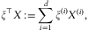$${{\xi }^ \top } \:X\::\: = \:\mathop{\sum}\limits_{i\: = \:1}^d {{\xi }^{(i)}} {{X}^{(i)}}, $$

where ξ = (ξ ⁽¹⁾, …, ξ ^(d)) is a vector of portfolio weights. If not mentioned otherwise, all vectors in $$${{{\Bbb R}}^d} $$$ will be regarded as column vectors. In particular, ξ = (ξ ⁽¹⁾, …, ξ ^(d)) actually means ξ = (ξ ⁽¹⁾, …, ξ ^(d))^⊤. To keep the writing as simple as possible, the transposition operation (·)^⊤ will be mentioned explicitly only if really necessary.

According to the intuition of diversifying a unit capital over different assets, we restrict ξ to the hyperplane

$${{H}_1}\::\: = \:\left\{ {x\: \in \:{{{\Bbb R}}^d} \::\:{{x}^{(1)}} \: + \: \ldots \: + \:{{x}^{(d)}} \: = \:1} \right\}.$$

Additional constraints on the portfolio weights can be implemented by restriction of ξ to smaller subsets of H ₁. A particularly important special case is the exclusion of negative portfolio weights, so-called short positions. The corresponding portfolio set is the unit simplex:

$${{{\rm{\rSigma }}}^d} \::\: = \:\left\{ {x\: \in \:{\Bbb R}_{ + }^{d} \::\:{{x}^{(1)}} \: + \ldots + \:{{x}^{(d)}} \: = \:1} \right\}.$$

2.2 Multivariate regular variation

Aiming at dependence of extremes, we assume that the probability distribution of X features a non-trivial dependence structure in the tails. This assumption is made precise in the following definition.

Definition 2.1 A random vector X in $$${{{\Bbb R}}^d} $$$ is multivariate regularly varying ($$${\cal M}{\cal R}{\cal V} $$$), if, as t → ∞,

$${\cal L}\left( {({{t}^{{\rm{ - }}1}} \:\parallel \:X\:\parallel \:,\:\parallel \:X\:\parallel {{\:}^{{\rm{ - }}1}} X)\, |\, \parallel \:X\:\parallel \: \gt \:t} \right){\mathop{ \rightarrow }\limits^{{\rm{w}}}} {{\rho }_\alpha } \otimes {\rm{\rPsi }}$$

where ρ_α is the Pareto(α) distribution, i.e., ρ_α((x,∞)): = x ^−α for x ≥ 1, and Ψ is a probability measure on the $$$ \parallel \cdot \parallel $$$-unit sphere $$$ {\Bbb S}_{{\parallel \cdot \parallel }}^{d} \::\: = \:\left\{ {s\: \in \:{{{\Bbb R}}^d} \::\parallel s\parallel \: = \:1} \right\} $$$.

The parameter α > 0 is called tail index of X, and the measure Ψ in (1) is called spectral or angular measure of X. In the sequel we will use the short notation X ∈ $$${\cal M}{\cal R}{\cal V}$$$_{−α ,Ψ} for multivariate regular variation with tail index α and spectral measure Ψ.

It is obvious that X ∈ $$${\cal M}{\cal R}{\cal V}$$$_{−α ,Ψ} entails univariate regular variation of $$$ \parallel X\parallel $$$ with same tail index α. That is, the distribution function $$$ {{F}_{\parallel X\parallel }} $$$ of $$$ \parallel X\parallel $$$ satisfies

$$\forall r\: \gt \:0\; \; \mathop {\lim }\limits_{t \rightarrow \infty } \frac{{1{\rm{ - }}{{F}_{\parallel X\parallel }}(tr)}}{{1{\rm{ - }}{{F}_{\parallel X\parallel }}(t)}}\: = \:{{r}^{{\rm{ - }}\alpha }} .$$

We will also use the short writing $$$ \parallel X\parallel \: \in \:{\cal R}{{{\cal V}}_{{\rm{ - }}\alpha }} $$$ for this property. It is well known that the tail index α separates finite moments from the infinite ones: (2) implies that $$$ {\rm{E}}\parallel X{{\parallel }^\beta } \: \lt \:\infty $$$ for β < α and $$$ {\rm{E}}\parallel X{{\parallel }^\beta } \: = \:\infty $$$ for β > α. Regular variation of random variables taking positive and negative values can be considered for the upper and the lower tail separately.

Moreover, X ∈ $$${\cal M}{\cal R}{\cal V}$$$_{−α ,Ψ} implies $$$ &#x007C;{{X}^{(i)}} &#x007C;\: \in \:{\cal R}{{{\cal V}}_{{\rm{ - }}\alpha }} $$$ for all i if

$$\forall i\: \in \:\{ 1, \ldots, d\} \; \; {\rm{\rPsi }}\left( {\left\{ {s\: \in \:{\Bbb S}_{{\parallel \cdot \parallel }}^{d} \::\:{{s}^{(i)}} \: = \:0} \right\}} \right)\: \lt \:1.$$

This non-degeneracy condition guarantees that all components X ⁽ⁱ⁾ are relevant to the extremes of the portfolio loss $$$ {{\xi }^ \top } X $$$. It should also be noted that X ∈ $$${\cal M}{\cal R}{\cal V}$$$_{−α ,Ψ} implies $$$ {{\xi }^ \top } X\, \in \,{\cal R}{{{\cal V}}_{{\rm{ - }}\alpha }} $$$ for all ξ under appropriate non-degeneracy conditions in the spirit of (3). For further details and for inverse results of Cramér-Wold type we refer to Basrak et al. (Reference Basrak, Davis and Mikosch2002) and Boman & Lindskog (Reference Boman and Lindskog2009).

The $$${\cal M}{\cal R}{\cal V} $$$ property can also be defined without polar coordinates. One can start with the assumption that there exists a sequence a_n→∞ and a (non-zero) Radon measure ν on the Borel σ-field $$$ {\cal B}([{\rm{ - }}\infty, \infty {{]}^d} \:\backslash \:\{ 0\} ) $$$ such that $$$ \nu ([{\rm{ - }}\infty, \infty {{]}^d} \backslash {{{\Bbb R}}^d} )\: = \:0 $$$ and, as n→∞,

$$n{{{\rm{P}}}^{a_{n}^{{{\rm{ - }}1}} X}} {\mathop{ \rightarrow }\limits^{{\rm{v}}}} \nu \ {\rm{on}}\,\,\,{\cal B}\left( {{{{[{\rm{ - }}\infty, \infty ]}}^d} \:\backslash \:\{ 0\} } \right),$$

where $$$ {\mathop{ \rightarrow }\limits^{{\rm{v}}}} $$$ denotes the vague convergence of Radon measures and $$$ {{{\rm{P}}}^{a_{n}^{{{\rm{ - }}1}} X}} $$$ is the probability distribution of $$$ a_{n}^{{{\rm{ - }}1}} X $$$. (cf. Resnick, Reference Resnick2007). This formulation is more technical than (1), but the measure ν in (4) is a very useful object. It is unique except for a multiplicative factor and exhibits the scaling property

$$\forall t\: \gt \:0\; \; \nu (tA)\: = \:{{t}^{{\rm{ - }}\alpha }} \nu (A),$$

which is the key to the most applications of $$${\cal M}{\cal R}{\cal V} $$$ models. It already implies that $$$ \nu \: = \:(c{{\bar{\rho }}_\alpha } \otimes {\rm{\rPsi }}) \circ \tau $$$ where $$$ \tau (x):\: = \:(\parallel x\parallel, \parallel x{{\parallel }^{{\rm{ - }}1}} x) $$$ is the polar coordinate transform, $$$ {{\bar{\rho }}_\alpha }((x,\infty ]):\: = \:{{x}^{{\rm{ - }}\alpha }} $$$ is an extension of ρ_α to (0,∞], and c > 0 is a constant. One can always obtain c = 1 by choosing $$$ {{a}_n}\: = \:F_{{\parallel X\parallel }}^{ \leftarrow } (1{\rm{ - }}1/n) $$$ where $$$ F_{{\parallel X\parallel }}^{ \leftarrow } $$$ is the quantile function of $$$ \parallel X\parallel $$$. We assume this standardization of ν throughout the following.

The measure ν also provides a link to the multivariate Extreme Value Theory. If

$$\nu \left( {\left\{ {x\: \in \:{{{\Bbb R}}^d} \::\:{{x}^{(i)}} \: \gt \:1} \right\}} \right)\: \gt \:0,\; \; i\: = \:1, \ldots, d,$$

then ν also characterizes the asymptotic distribution of the componentwise maxima $$$ {{M}_n}\::\: = \:({{M}^{(1)}}, \ldots, {{M}^{(d)}} ) $$$ with $$$ {{M}^{(i)}} \::\: = \:\max \{ X_{1}^{{(i)}}, \ldots, X_{n}^{{(i)}} \} $$$. An equivalent writing of (6) is $$$ {\rm{\rPsi }}(\{ s \in {\Bbb S}_{{\parallel \cdot \parallel }}^{d} :{{s}_i}\: \gt \:0\} )\: \gt \:0 $$$ for all i, which is a special case of (3). This assumption implies that

$${\rm{P}}\left\{ {a_{n}^{{{\rm{ - }}1}} {{M}_n}\: \in \:[{\rm{ - }}\infty, x]} \right\}{\mathop{ \rightarrow }\limits^{{\rm{w}}}} \exp \left( {{\rm{ - }}\nu \left( {{{{[{\rm{ - }}\infty, \infty ]}}^d} \:\backslash \:[{\rm{ - }}\infty, x]} \right)} \right)$$

for x ∈ (0,∞]^d and $$$ {{a}_n}\: = \:F_{{\parallel X\parallel }}^{ \leftarrow } (1{\rm{ - }}1/n) $$$. Therefore ν is also called exponent measure. For further details on the asymptotic distributions of maxima see Resnick (Reference Resnick1987) and Haan & Ferreira (Reference Ferreira2006).

Although the domain of Ψ depends on the norm underlying the polar coordinates, the $$${\cal M}{\cal R}{\cal V} $$$ property is norm-independent in the following sense: if (1) holds for some norm $$$ \parallel \cdot \parallel $$$, then it holds also for any other norm $$$ \parallel \cdot {{\parallel }_\diamondsuit } $$$ that is equivalent to $$$ \parallel \cdot \parallel $$$. In this paper we use the sum norm $$$ \parallel x{{\parallel }_1}:\: = \:\mathop{\sum}\sidelimits_{i\: = \:1}^d &#x007C;{{x}^{(i)}} &#x007C; $$$ and let Ψ denote the spectral measure on the unit sphere $$$ {\Bbb S}_{1}^{d} $$$ induced by $$$ \parallel \cdot {{\parallel }_1} $$$. In the special case of $$$ {\Bbb R}_{ + }^{d} $$$-valued random vectors it may be convenient to reduce the domain of Ψ to $$$ {\Bbb S}_{{\parallel \cdot \parallel }}^{d} \: \cap \:{\Bbb R}_{ + }^{d} $$$. For $$$ {\Bbb S}_{1}^{d} $$$ this is the unit simplex Σ^d.

Further details on regular variation of functions or random variables can be found in Bingham et al. (Reference Bingham, Goldie and Teugels1987), Resnick (Reference Resnick1987), Basrak et al. (Reference Basrak, Davis and Mikosch2002), Mikosch (Reference Mikosch2003), Hult & Lindskog (Reference Hult and Lindskog2006), Haan & Ferreira (Reference Ferreira2006), Resnick (Reference Resnick2007).

2.3 Portfolio loss asymptotics

The $$${\cal M}{\cal R}{\cal V} $$$ assumption has strong consequences on the asymptotic behaviour of large portfolio losses. It allows to assess the asymptotics of the Value-at-Risk VaR_λ and the Expected Shortfall ES_λ for $$$ \lambda \nearrow 1 $$$, i.e., far out in the tail. The next result provides a general characterization of the asymptotic portfolio losses in multivariate regularly varying models. The special case of random vectors in $$$ {\Bbb R}_{ + }^{d} $$$ was studied in Mainik & Rüschendorf (Reference Mainik and Rüschendorf2010). The general case is treated in Mainik (Reference Mainik2010, Lemma 3.2).

(a)

$$\mathop {\lim }\limits_{t \rightarrow \infty } \; \; \frac{{{\rm{P}}\{ {{\xi }^{\rm \top}} X\: \gt \:t\} }}{{{\rm{P}}\{ \parallel X{{\parallel }_1}\: \gt \:t\} }}\: = \:{{\gamma }_\xi }:\: = \:{\int}_{{\!\!\!\!\Bbb S}_{1}^{d} } ({{\xi }^{\rm \top}} s)_{ + }^{\alpha } \:{\rm{d\rPsi }}(s);$$

(b)

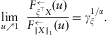$$\mathop {\lim }\limits_{u \nearrow 1} \; \; \frac{{F_{{{{\xi }^{\rm \top}} X}}^{ \leftarrow } (u)}}{{F_{{\parallel X{{\parallel }_1}}}^{ \leftarrow } (u)}}\: = \:\gamma _{\xi }^{{1/\alpha }} .$$

The immediate consequence of (8) and (9) is that the functional γ_ξ characterizes the asymptotics of portfolio loss probabilities and the corresponding high loss quantiles. In particular, the limit relation (9) allows for an asymptotic comparison of the Value-at-Risk associated with different portfolio vectors ξ. The Value-at-Risk VaR_λ(Y) of a random loss Y is defined as the λ-quantile of Y (cf. McNeil et al. Reference McNeil, Frey and Embrechts2005):

$${\rm{Va}}{{{\rm{R}}}_\lambda }(Y):\: = \:F_{Y}^{ \leftarrow } (\lambda ).$$

In the context of diversification effects, the basic question is the comparison of portfolio losses $$$ \xi _{1}^{ \top } X $$$ and $$$ \xi _{2}^{ \top } X $$$ for standardized portfolio vectors ξ ₁, ξ ₂ ∈ H ₁. From (10) we immediately obtain an asymptotic comparison of the portfolio VaR.

Corollary 2.3. Let X ∈ $$${\cal M}{\cal R}{\cal V}$$$_{−α ,Ψ}and ξ ₁, ξ ₂ ∈ H ₁. Then

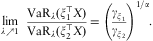$$\mathop {\lim }\limits_{\lambda \nearrow 1} \; \; \frac{{{\rm{Va}}{{{\rm{R}}}_\lambda }(\xi _{1}^{{\rm \top}} X)}}{{{\rm{Va}}{{{\rm{R}}}_\lambda }(\xi _{2}^{{\rm \top}} X)}}\: = \:{{\left( {\frac{{{{\gamma }_{{{\xi }_1}}}}}{{{{\gamma }_{{{\xi }_2}}}}}} \right)}^{1/\alpha }} .$$

Analogous comparison results for the Expected Shortfall ES_λ and other spectral risk measures are also possible (cf. Mainik & Rüschendorf, Reference Mainik and Rüschendorf2010).

A particularly important case is ξ ₂ = e_i, where e_i is the i-th unit vector for i∈{1, …, d}. This portfolio vector represents the single asset strategy investing all capital in the i-th asset. The ratio γ_ξ/γ_ei is well defined if γ_ei > 0. If γ_ei = 0 for some i, then the risk optimal portfolio cannot contain any asset j with γ_ej > 0. The non-degeneracy assumption (6) is equivalent to γ_ei > 0 for all i. It keeps the losses of all assets on the same scale and focuses the discussion on the non-trivial cases. Henceforth we assume (6) to be satisfied.

2.4 Sub- and superadditivity

The limit relation (11) links asymptotic subadditivity of VaR to the functional $$$ \gamma _{\xi }^{{1/\alpha }} $$$. Indeed, we can write $$$ {{X}^{(i)}} \: = \:e_{i}^{ \top } X $$$ and $$$ {{X}^{(1)}} \: + \:{{X}^{(2)}} \: = \:2{{\eta }^ \top } X $$$ with $$$ \eta :\: = \:\left( {\frac{1}{2},\frac{1}{2}} \right) $$$. Applying (11), we obtain that

$$\frac{{{\rm{Va}}{{{\rm{R}}}_\lambda }({{X}^{(1)}} \: + \:{{X}^{(2)}} )}}{{{\rm{Va}}{{{\rm{R}}}_\lambda }({{X}^{(1)}} )\: + \:{\rm{Va}}{{{\rm{R}}}_\lambda }({{X}^{(2)}} )}} \rightarrow \frac{{\gamma _{{\left( {\frac{1}{2},\frac{1}{2}} \right)}}^{{1/\alpha }} }}{{\tfrac{1}{2}\gamma _{{{{e}_1}}}^{{1/\alpha }} \: + \:\tfrac{1}{2}\gamma _{{{{e}_2}}}^{{1/\alpha }} }}.$$

Thus we see that checking the asymptotic subadditivity of VaR for X = (X ⁽¹⁾, X ⁽²⁾) is related to the comparison of $$$ \gamma _{\eta }^{{1/\alpha }} $$$ and $$$ {{\eta }^{(1)}} \gamma _{{{{e}_1}}}^{{1/\alpha }} \: + \:{{\eta }^{(2)}} \gamma _{{{{e}_2}}}^{{1/\alpha }} $$$.

A more general approach is the analysis of the mapping $$$ \xi \, \mapsto \,\rho ({{\xi }^{\rm \top}} X) $$$ for some risk measure ρ. Extending from the equally weighted portfolio η to ξ ∈ Σ^d, we see that the asymptotic subadditivity of VaR_λ for $$$ \lambda \nearrow 1 $$$ is related to the inequality

$$\gamma _{\xi }^{{1/\alpha }} \:\leq \:\mathop{\sum}\limits_{i\: = \:1}^d {{\xi }^{(i)}} \gamma _{{{{e}_i}}}^{{1/\alpha }} .$$

That is, we need to know whether the mapping $$$ \xi \, \mapsto \,\gamma _{\xi }^{{1/\alpha }} $$$ is convex on the unit simplex Σ^d. In terms of diversification, convexity of $$$ \gamma _{\xi }^{{1/\alpha }} $$$ means that a mixed portfolio is typically better than a one-asset strategy.

The convexity of $$$ \gamma _{\xi }^{{1/\alpha }} $$$ is related to the Minkowski inequality on the function space $$$ {{L}^\alpha } ({\rm{\rPsi }}) $$$. This was already pointed out by Embrechts et al. (Reference Embrechts, Lambrigger and Wüthrich2009) in a slightly different setting related to the aggregation of risks. Applying (8), one immediately obtains that

$$\gamma _{\xi }^{{1/\alpha }} = \parallel {{h}_\xi }{{\parallel }_{{\rm{\rPsi }},\alpha }}$$

with $$$ {{h}_\xi }(s):\: = \:{{({{\xi }^{\rm \top}} s)}_ + } $$$ and $$$ \parallel f{{\parallel }_{{\rm{\rPsi }},\alpha }}:\: = \:{{(\int {{f}^\alpha } {\rm{d\rPsi }})}^{1/\alpha }} $$$. Although $$$ \parallel \cdot {{\parallel }_{\rPsi, \alpha }} $$$ is not a norm for α < 1, one still can define function spaces L ^α(Ψ) as collections of all measurable functions $$$ f:{\Bbb S}_{1}^{d} \: \rightarrow \:{\Bbb R} $$$ such that $$$ \parallel f{{\parallel }_{\rPsi, \alpha }}\, \lt \,\infty $$$. We demonstrate below that the missing triangle inequality for $$$ \parallel \cdot {{\parallel }_{\rPsi, \alpha }} $$$ is the origin of asymptotic risk superadditivity in $$${\cal M}{\cal R}{\cal V} $$$ models with α < 1.

The next theorem summarizes the diversification properties in the special case Ψ(Σ^d) = 1, as it occurs for random vectors in $$$ {\Bbb R}_{ + }^{d} $$$. For $$$ {\Bbb R}_{{}}^{d} $$$-valued random vectors, Ψ(Σ^d) = 1 means that the excess behaviour of the gains is weaker than that of the losses, so that compensation of high losses by high gains is impossible. This setting is typical for risk aggregation in insurance and reinsurance, with small incremental premia constantly coming in and potentially large losses from rare events. In financial applications, risk aggregation without loss-gain compensation is particularly important in the area of operational risk.

1. (a) convex for α > 1;

2. (b) linear for α = 1;

3. (c) concave for α < 1.

Proof. Let ξ ₁, ξ ₂∈Σ^d and λ∈(0, 1). Then

$$\forall s\: \in \:{{\rSigma }^d} \; \; {{h}_{\lambda {{\xi }_1}\: + \:(1{\rm{ - }}\lambda ){{\xi }_2}}}(s)\: = \:\lambda {{h}_{{{\xi }_1}}}\: + \:(1{\rm{ - }}\lambda ){{h}_{{{\xi }_2}}}.$$

Thus the case α = 1 is trivial and the rest follows from the Minkowski inequality for L ^p spaces with p∈(0,∞). The standard case p ≥ 1 is well known, whereas for p < 1 and non-negative functions the inequality is inverse. (cf. Hardy et al. Reference Hardy, Littlewood and Pólya1934, Theorem 2.24, p.30). □

There are two general conclusions from Theorem 2.4. On the one hand, if the $$${\cal M}{\cal R}{\cal V} $$$ assumption accords with the real world data and α is greater than 1, then one can expect VaR_λ to be subadditive for λ close to 1. Although appropriate choice of dependence structure for given marginal distributions always allows to violate the subadditivity of VaR (cf. McNeil et al. Reference McNeil, Frey and Embrechts2005, Example 6.22, and Embrechts & Puccetti, Reference Embrechts and Puccetti2010), $$${\cal M}{\cal R}{\cal V} $$$ excludes these pathological cases at least in the asymptotic sense. On the other hand, if α < 1 and the $$${\cal M}{\cal R}{\cal V} $$$ assumption fits the reality, then diversification is generally bad for any asymptotic dependence structure Ψ on Σ^d. Surprising as it may appear at the first glance, this phenomenon has an intuitive explanation. The mathematical background of diversification is the Law of Large Numbers, which essentially means that the fluctuation of averages is lower than that of separate random variables. If the expectations are infinite, this reasoning breaks down. In the insurance context, this means that sharing catastrophic risks may increase the danger of insolvency. In the context of operational risk data having a tail index below 1, the increased financial power of a larger bank may still be insufficient to compensate the increased intensity of operational losses. With infinite means in the risk data, one can only reduce the total risk by reducing the number of risk exposures.

The next theorem summarizes the diversification properties in the general case, where Ψ is not concentrated on Σ^d. This setting allows the gains to be on the same scale with losses, so that loss-gain compensation can take place in the tail region.

1. (a) continuous;

2. (b) convex for α ≥ 1.

Proof. Part (a). As s∈Σ^d is bounded, the mapping $$$ \xi \, \mapsto \,{{h}_\xi }(s) $$$ is continuous uniformly in s∈Σ^d. This implies the continuity of the mapping $$$ \xi \, \mapsto \,\parallel {{h}_\xi }{{\parallel }_{{\rm{\rPsi }},\alpha }} $$$.

Part (b). Let $$$ {{\xi }_1},{{\xi }_2}\: \in \:{\Bbb S}_{1}^{d} $$$ and λ ∈ (0,1). The convexity of the mapping $$$ t\, \mapsto \,{{t}_ + } $$$ yields

$$\forall s\: \in \:{{\rSigma }^d} \; \; {{h}_{\lambda {{\xi }_1}\: + \:(1{\rm{ - }}\lambda ){{\xi }_2}}}(s)\:\leq \:\lambda {{h}_{{{\xi }_1}}}(s)\: + \:(1{\rm{ - }}\lambda ){{h}_{{{\xi }_2}}}(s).$$

The result follows from the Minkowski inequality. □

Compared to Theorem 2.4, the most important difference in Theorem 2.6 is the missing statement for α < 1. This is not only because the techniques used before do not apply here. Diversification effects for α < 1 in models with loss-gain compensation are much more complex than in the pure loss setting. The crucial factor here is the tail dependence structure, i.e., the spectral measure Ψ. For some Ψ one can have convexity, for some others piecewise concavity. Models that appear similar at a first glance turn out to have very different VaR asymptotics. Some of these modelling traps and the resulting confusion will be discussed in the next section.

3.1 Catastrophic risks: dependence vs. independence

According to Theorem 2.4, superadditivity of portfolio risks is inevitable if α < 1 and the losses cannot be compensated by gains. In addition to that, it turns out that the influence of dependence on the diversification effects is inverse in this case. That is, lower dependence of risk components X ⁽ⁱ⁾ increases the risk of any portfolio $$$ {{\xi }^ \top } X $$$ for ξ ∈ Σ^d. The upper bound for asymptotic portfolio risk is attained by the random vector with independent components, whereas the lower bound is achieved by taking all risk components equal. This inverse ordering of diversification effects for α < 1 was shown by Mainik & Rüschendorf (Reference Mainik and Rüschendorf2012).

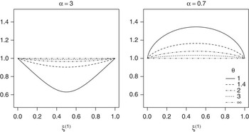
Figure 1 shows the diversification effects arising in a bivariate regularly varying model with a Gumbel copula C_ϑ and identically distributed, non-negative, regularly varying margins X ⁽ⁱ⁾. The dependence parameter ϑ ranges from 1 to ∞, thus covering both extremal cases: the independence (ϑ = 1) and the monotonicity (ϑ = ∞). To make the diversification effect curves comparable, the portfolio risk functional is normalized according to (11). That is, the plots show the asymptotic VaR ratio of the portfolio ξ $$$^\top$$$X and the single asset X ⁽¹⁾:

$$\gamma {{_{\xi }^{ \ast } }^{1/\alpha }} :\: = \:{{\left( {\frac{{{{\gamma }_\xi }}}{{{{\gamma }_{{{e}_1}}}}}} \right)}^{1/\alpha }} \: = \:\mathop {\lim }\limits_{\lambda \nearrow 1} \frac{{{\rm{Va}}{{{\rm{R}}}_\lambda }({{\xi }^{\rm \top}} X)}}{{{\rm{Va}}{{{\rm{R}}}_\lambda }({{X}^{(1)}} )}}.$$

Figure 1

The asymptotic VaR ratio $$$ \gamma {{_{\xi }^{ \ast } }^{1/\alpha }} $$$ for $$${\cal M}{\cal R}{\cal V} $$$ models with a Gumbel copula: diversification is bad for α < 1.

The ordering of the asymptotic risk profiles $$$ \gamma {{_{\xi }^{ \ast } }^{1/\alpha }} $$$ with respect to the dependence parameter ϑ suggests a uniform ordering of diversification effects for ξ ∈ Σ^d. The direction of this ordering depends on α: smaller ϑ improves the diversification effects for α > 1, but increases the portfolio risk for α < 1. For the calculation of $$$ \gamma _{\xi }^{ \ast } $$$ in this model and a mathematical proof of the ordering result see Mainik & Rüschendorf (Reference Mainik and Rüschendorf2012).

The inverse diversification effects for α < 1 and the inverse impact of dependence on the portfolio risk illustrated in Figure 1 are typical for regularly varying models in $$$ {\Bbb R}_{ + }^{d} $$$. Moreover, the parameter values ϑ = 1 and ϑ = ∞ represent ultimate bounds for diversification effects that can be attained at any dependence structure (cf. Mainik & Rüschendorf, Reference Mainik and Rüschendorf2012). In particular, additive VaR is the best case one can have for α < 1.

3.2 Elliptical distributions

An important class of stochastic models is that of elliptical distributions. It can be considered as a generalization of the multivariate Gaussian distribution that preserves the elliptical shape of sample clouds but allows for non-Gaussian tails. In particular, the standard variance-covariance aggregation rules for VaR remain valid for all elliptical distributions (cf. McNeil et al. Reference McNeil, Frey and Embrechts2005, Theorem 6.8).

A random vector X in $$$ {\Bbb R}_{{}}^{d} $$$ is elliptically distributed if it satisfies

$$X\,{\mathop{ = }\limits^{{\rm{d}}}} \,\mu \, + \,RAU,$$

where μ ∈ $$$ {\Bbb R}_{{}}^{d} $$$, A ∈ $$$ {\Bbb R}_{{}}^{{d\times d}} $$$, U is uniformly distributed on the Euclidean sphere $$$ {\Bbb S}_{2}^{d} $$$, and R is a non-negative random variable that is independent of U. If ER < ∞, then EX = μ, and if ER ² < ∞, then the covariance matrix of X is given by

$${\rm{E}}\left( {(X{\rm{ - }}\mu )(X{\rm{ - }}\mu {{)}^ \top } } \right)\: = \:{\rm{E}}\left( {{{R}^2} AU{{U}^ \top } {{A}^ \top } } \right)\: = \:{\rm{E}}{{R}^2} A{{A}^ \top } .$$

The matrix $$$C:\: = A{{A}^ \top } $$$ is called ellipticity matrix of X. It is unique except for a constant factor. Given a symmetric and positive semidefinite matrix C, we can always find A such that C = $$$ A{{A}^ \top } $$$ by Cholesky decomposition.

For elliptically distributed X, X ∈ $$${\cal M}{\cal R}{\cal V}$$$ is equivalent to R ∈ $$${\cal R}{\cal V}$$$_−α for some α > 0 (cf. Hult & Lindskog, Reference Hult and Lindskog2002). To exclude degenerate cases, we assume throughout the following that C is positive definite. The spectral measure of X depends on C and α. Explicit formulas for the spectral density in the bivariate case are derived in Hult & Lindskog (Reference Hult and Lindskog2002), and a general representation for d ≥ 2 is given in Mainik (Reference Mainik2010).

However, the calculation of the asymptotic risk profile $$$ \gamma {{_{\xi }^{ \ast } }^{1/\alpha }} $$$ for elliptical distributions can be carried out without spectral measures. Let a: = ξ ^⊤A. Then

$${{\xi }^ \top } X\,{\mathop{ = }\limits^{{\rm{d}}}} \,{{\xi }^ \top } \mu \, + \:\parallel a{{\parallel }_2}R{{(\parallel a\parallel _{2}^{{{\rm{ - }}1}} a)}^ \top } U.$$

By symmetry of $$$ {\Bbb S}_{2}^{d} $$$ we have that $$$ {{(\parallel a\parallel _{2}^{{{\rm{ - }}1}} a)}^ \top } U\,{\mathop{ = }\limits^{{\rm{d}}}} \,e_{1}^{ \top } U\, = \,{{U}^{(1)}} $$$. This gives

$${{\xi }^ \top } X\,{\mathop{ = }\limits^{{\rm{d}}}} \,{{\xi }^ \top } \mu \, + \,\parallel {{\xi }^ \top } A{{\parallel }_2}Z$$

with $$$ Z\,{\mathop{ = }\limits^{{\rm{d}}}} \,R{{U}^{(1)}} $$$.

Hence $$$ {\rm{Va}}{{{\rm{R}}}_\lambda }({{\xi }^ \top } X)\: = \:{{\xi }^ \top } \mu \: + \:\parallel {{\xi }^ \top } A{{\parallel }_2}F_{Z}^{ \leftarrow } (\lambda ) $$$. As $$$ F_{Z}^{ \leftarrow } (\lambda )\: \rightarrow \:\infty $$$ for $$$ \lambda \nearrow 1 $$$, we obtain from (11) that

$$\gamma {{_{\xi }^{ \ast } }^{1/\alpha }} \: = \:{{\left( {\frac{{{{\gamma }_\xi }}}{{{{\gamma }_{{{e}_1}}}}}} \right)}^{1/\alpha }} \: = \:\mathop {\lim }\limits_{t\: \rightarrow \:\infty } \frac{{{{\xi }^ \top } \mu \: + \:t\parallel {{\xi }^ \top } A{{\parallel }_2}}}{{{{\mu }^{(1)}} \: + \:t\parallel e_{1}^{ \top } A{{\parallel }_2}}}\: = \:\sqrt {{{\xi }^ \top } C\xi /{{C}_{1,1}}} .$$

It is also easy to see that this diversification effect is non-asymptotic for all centred elliptical distributions with any R (not necessarily regularly varying). That is, for μ = 0 and $$$ \lambda \: \in \:\left( {\frac{1}{2},1} \right) $$$ we always have

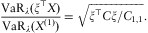$$\frac{{{\rm{Va}}{{{\rm{R}}}_\lambda }({{\xi }^ \top } X)}}{{{\rm{Va}}{{{\rm{R}}}_\lambda }({{X}^{(1)}} )}}\: = \:\sqrt {{{\xi }^ \top } C\xi /{{C}_{1,1}}} .$$

This is exactly the variance-covariance VaR aggregation rule, which was originally derived in the Gaussian setting.

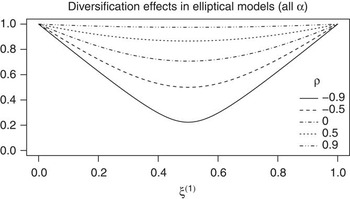
Figure 2 shows plots of this ratio in the bivariate setting with $$$ { {C}\: = \:\left( {\matrix{ 1 &amp; \rho \cr \rho &amp; 1 }}\right)$$$ for different values of ρ. In particular, the asymptotic diversification effect $$$ \gamma {{_{\xi }^{ \ast } }^{1/\alpha }} \: = \:{{({{\gamma }_\xi }/{{\gamma }_{{{e}_1}}})}^{1/\alpha }} $$$ does not depend on α if X is elliptical. Moreover, we have a uniform ordering of portfolio risks in the sense that lower ρ implies lower portfolio risk for any ξ ∈ Σ^d. This remarkable property is a consequence of the geometric structure of elliptical distributions. On the other hand, the asymptotic ratio of excess probabilities for different portfolios depends on α. Applying (8), we immediately obtain that

$$\mathop {\lim }\limits_{t \rightarrow \infty } \frac{{{\rm{P}}({{\xi }^ \top } X\: \gt \:t)}}{{{\rm{P}}({{X}^{(1)}} \: \gt \:t)}}\: = \:\frac{{{{\gamma }_\xi }}}{{{{\gamma }_{{{e}_1}}}}}\: = \:{{\left( {{{\xi }^ \top } C\xi /{{C}_{1,1}}} \right)}^{\alpha /2}} .$$

Figure 2

The asymptotic VaR ratio $$$ \gamma {{_{\xi }^{ \ast } }^{1/\alpha }} $$$ for elliptical distributions does not depend on α.

Plots of this ratio are shown in Figure 3.

Figure 3

Asymptotic excess probabilities may be misleading: γ_ξ/γe ₁ for elliptical distributions depends on α (whereas $$$ \gamma {{_{\xi }^{ \ast } }^{1/\alpha }} \: = \:{{({{\gamma }_\xi }/{{\gamma }_{{{e}_1}}})}^{1/\alpha }} $$$ does not).

3.3 Heavy-tailed linear models are not elliptical

An appealing property of multivariate Gaussian models is their interpretation in terms of linear regression. In the bivariate case this essentially means that a bivariate Gaussian random vector X = (X ⁽¹⁾, X ⁽²⁾) with margins $$$ {{X}^{(1)}}, \,{{X}^{(2)}} \: \sim \:{\cal N}(0,1) $$$ and correlation ρ ∈ (−1, 1) satisfies

$${{X}^{(2)}} \: = \:\rho {{X}^{(1)}} \: + \:\sqrt {1{\rm{ - }}{{\rho }^2} } \, {{Y}^{(2)}}, $$

where $$$ {{Y}^{(2)}} \: \sim \:{\cal N}(0,1) $$$, independent of X ⁽¹⁾. Setting Y ⁽¹⁾ := X ⁽¹⁾ and Y := (Y ⁽¹⁾, Y ⁽²⁾)^⊤, we can write it as

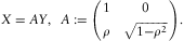$${X\: = \:AY,\; \; A:\: = \left( {\matrix{ 1 &amp; 0 \cr \rho &amp;{\sqrt {1{\rm{ - }}{{\rho }^2} } } }}\right).$$

That is, X can be obtained as a linear transformation of a random vector with independent margins. The generation of $$$ X\: \sim \:{\cal N}(0,C) $$$ for an arbitrary covariance matrix C∈$$${{{\Bbb R}}^{d\times d}} $$$ uses (13). It suffices to choose A such that $$$ A{{A}^ \top } $$$ = C. As $$$ {\cal N}(0, C) $$$ is elliptical with ellipticity matrix C, the diversification effects in the model (13) are the same as in Figure 2.

However, the Gaussian case is the only one where the linear model (13) with independent Y ⁽ⁱ⁾ is elliptical. To demonstrate the difference between elliptical and linear models in the heavy-tailed case, we compare the multivariate elliptical Student-t distribution with the model generated according to (13) from Y with independent t-distributed margins. The same heavy-tailed linear model was used by Daníelsson et al. (Reference Daníelsson, Jorgensen, Samorodnitsky and Sarma2005), Daníelsson et al. (Reference Daníelsson, Jorgensen, Samorodnitsky and Sarma2012) in simulation studies on risk sub- and superadditivity. The simulation results obtained there deviated strongly from what one would expect in an elliptical model. In particular, the VaR subadditivity depended on the tail index α, which should not be the case for an elliptical t distribution. The analysis presented below will explain the simulation results of Daníelsson et al. (Reference Daníelsson, Jorgensen, Samorodnitsky and Sarma2005) and give additional insight into the behaviour of VaR in $$${\cal M}{\cal R}{\cal V} $$$ models with α < 1.

Let X = AY with A from (13) and assume that the margins Y ⁽¹⁾,Y ⁽²⁾ of Y are independent Student-t distributed with degrees of freedom equal to α > 0. Note that $$$ {\rm{E}}({{Y}^{(i)}} ^{2} )\, \lt \,\infty $$$ for α > 2. In this case, the correlation matrix of X is well defined and given by

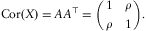$${\rm{Cor}}(X)\: = \:A{{A}^ \top } \: = \left( {\matrix{ 1 &amp; \rho \cr \rho &amp; 1 }}\right).$$

The generation of elliptical t random vectors is quite easy. Let W ⁽¹⁾,W ⁽²⁾, V be independent random variables with $$$ {{W}^{(i)}} \: \sim \:{\cal N}(0,1) $$$ and V∼χ² with α degrees of freedom. Then the random vector

$$Z:\: = \:\sqrt {\frac{\alpha }{V}} \, AW,\; \; W\: = \:{{\left( {{{W}^{(1)}}, {{W}^{(2)}} } \right)}^ \top } $$

is elliptically distributed with Z⁽ⁱ⁾∼t(α), i = 1, 2 (cf. McNeil et al. Reference McNeil, Frey and Embrechts2005, Example 3.7). The ellipticity matrix is equal to C, which is also Cor(Z) for α > 2.

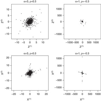
Figure 4 shows scatterplots of 1000 simulated i.i.d. observations of Z and X, respectively. Although Z and X have the same “correlation structure” (correlation is only defined for α > 2), the difference between the samples is remarkable. While large observations of Z concord with the elliptical shape of the sample cloud, the excess points of X are concentrated on two axes. This concentration gets stronger for heavier tails, i.e., for smaller α. The cross-shaped sample clouds indicate that the spectral measure of the linear heavy-tailed model (13) consists of four atoms. The calculation of this spectral measure is given in Appendix A.

Figure 4

Elliptical vs. linear t model with a degrees of freedom and “correlation” parameter ρ: 1000 simulated i.i.d. observations of the random vector Z defined in (14) and the random vector X = AY with Y ⁽ⁱ⁾ i.i.d. ∼t(α).

This property of the linear model originates from the polynomial tails of the t distribution. It is well known that the t(α) distribution is regularly varying with tail index α. Moreover, symmetry arguments give $$$ &#x007C;{{Y}^{(i)}} &#x007C;\: \in \:{\cal R}{{{\cal V}}_{{\rm{ - }}\alpha }} $$$, i.e., $$$ {{\bar{F}}_{&#x007C;{{Y}^{(i)}} &#x007C;}}(r)\, = \,{{r}^{{\rm{ - }}\alpha }} l(r) $$$ with some $$$ l\: \in \:{\cal R}{{{\cal V}}_0} $$$.

The asymptotic diversification effect $$$ \gamma {{_{\xi }^{ \ast } }^{1/\alpha }} $$$ can be calculated directly. It is obvious that $$$ e_{1}^{ \top } X\: = \:{{Y}^{(1)}} $$$ and

$${{\xi }^ \top } X\: = \:({{\xi }^{(1)}} \: + \:{{\xi }^{(2)}}\rho ){{Y}^{(1)}} \: + \:{{\xi }^{(2)}} \sqrt {1{\rm{ - }}{{\rho }^2} } \:{{Y}^{(2)}} .$$

Due to (8), regular variation and independence of Y ⁽ⁱ⁾ imply that

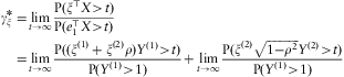$${ \gamma _{\xi }^{ \ast } \: = \: &amp; \mathop {\lim }\limits_{t\: \rightarrow \:\infty } \frac{{{\rm{P}}({{\xi }^ \top } X\: \gt \:t)}}{{{\rm{P}}(e_{1}^{{\rm \top}} X\: \gt \:t)}} \cr = &amp; \mathop {\lim }\limits_{t\: \rightarrow \:\infty } \frac{{{\rm{P}}(({{\xi }^{(1)}} \: + \:{{\xi }^{(2)}}\rho ){{Y}^{(1)}} \: \gt \:t)}}{{{\rm{P}}({{Y}^{(1)}} \: \gt \:1)}}\: + \:\mathop {\lim }\limits_{t\: \rightarrow \:\infty } \frac{{{\rm{P}}({{\xi }^{(2)}} \sqrt {1{\rm{ - }}{{\rho }^2} } \:{{Y}^{(2)}} \: \gt \:t)}}{{{\rm{P}}({{Y}^{(1)}} \: \gt \:1)}} \cr}$$

(cf. Embrechts et al. Reference Embrechts, Klüppelberg and Mikosch1997, Lemma 1.3.1). Moreover, from $$$ {{Y}^{(1)}} \,{\mathop{ = }\limits^{{\rm{d}}}} \,{{Y}^{(2)}} $$$ and Y ⁽²⁾∈$$${\cal R}{\cal V}$$$_−α we obtain that

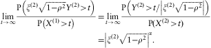$${ \mathop {\lim }\limits_{t \rightarrow \infty } \frac{{{\rm{P}}\left( {{{\xi }^{(2)}} \sqrt {1{\rm{ - }}{{\rho }^2} } \:{{Y}^{(2)}} \: \gt \:t} \right)}}{{{\rm{P}}\left( {{{X}^{(1)}} \: \gt \:t} \right)}}\: = \: &amp; \mathop {\lim }\limits_{t\: \rightarrow \:\infty } \frac{{{\rm{P}}\left( {{{Y}^{(2)}} \: \gt \:t\:/\:\left&#x007C; {{{\xi }^{(2)}} \sqrt {1{\rm{ - }}{{\rho }^2} } } \right&#x007C;} \right)}}{{{\rm{P}}({{X}^{(2)}} \: \gt \:t)}} \cr = &amp; {{\left&#x007C; {{{\xi }^{(2)}} \sqrt {1{\rm{ - }}{{\rho }^2} } } \right&#x007C;}^\alpha } . \cr}$$

Similar arguments yield

$${ \mathop {\lim }\limits_{t \rightarrow \infty } \frac{{{\rm{P}}(({{\xi }^{(1)}} \: + \:{{\xi }^{(2)}}\rho ){{Y}^{(1)}} \: \gt \:t)}}{{{\rm{P}}({{Y}^{(1)}} \: \gt \:1)}}\: = \: &amp; \mathop {\lim }\limits_{t \rightarrow \infty } \frac{{{\rm{P}}\left( {{{Y}^{(1)}} \: \gt \:t/\:&#x007C;\:{{\xi }^{(1)}} \: + \:{{\xi }^{(2)}} \rho &#x007C;} \right)}}{{{\rm{P}}({{Y}^{(1)}} \: \gt \:t)}} \cr = &amp; {{\left&#x007C; {{{\xi }^{(1)}} \: + \:{{\xi }^{(2)}} \rho } \right&#x007C;}^\alpha } . \cr} $$

Hence

$${{(\gamma _{\xi }^{ \ast } (X))}^{1/\alpha }} \: = \:{{\left( {{{{\left&#x007C; {{{\xi }^{(1)}} \: + \:{{\xi }^{(2)}} \rho } \right&#x007C;}}^\alpha } \: + \:{{{\left&#x007C; {{{\xi }^{(2)}} \sqrt {1{\rm{ - }}{{\rho }^2} } } \right&#x007C;}}^\alpha } } \right)}^{1/\alpha }} .$$

In contrast to the diversification effects in elliptical models, this expression depends on α. If ρ ≥ 0, then the function $$$ \xi \, \mapsto \,\gamma {{_{\xi }^{ \ast } }^{1/\alpha }} $$$ is convex for α ≥ 0 and concave for ρ ≤ 0. In particular, $$$ \gamma {{_{\xi }^{ \ast } }^{1/\alpha }} $$$ is linear in ξ for ρ ≥ 1 and α = 1. This means that VaR is asymptotically additive in this case:

$$\mathop {\lim }\limits_{\lambda \nearrow 1} \frac{{{\rm{Va}}{{{\rm{R}}}_\lambda }({{\xi }^ \top } X)}}{{{{\xi }^{(1)}} {\rm{Va}}{{{\rm{R}}}_\lambda }({{X}^{(1)}} )\: + \:{{\xi }^{(2)}} {\rm{Va}}{{{\rm{R}}}_\lambda }({{X}^{(2)}} )}}\: = \:1.$$

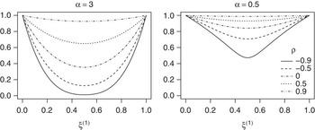
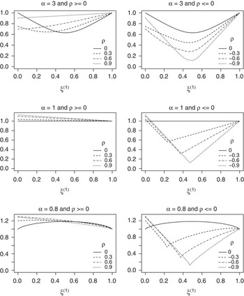
Figure 5 shows plots of the asymptotic risk profile $$$ \gamma {{_{\xi }^{ \ast } }^{1/\alpha }} $$$ in the linear model for selected values of α and ρ. If ρ < 0, then the asymptotic portfolio risk is piecewise linear for α = 1 and piecewise concave for α < 1. This demonstrates explicitly that the statements of Theorem 2.4(b, c) do not hold for X with $$$ {{{\rm{\rPsi }}}_X}({{\Sigma }^d} )\: \lt \:1 $$$.

Figure 5

Asymptotic VaR ratio $$$ \gamma {{_{\xi }^{ \ast } }^{1/\alpha }} $$$ in the linear heavy-tailed model.

This is extremely different from the elliptical t model, where the diversification effects are the same for all α (cf. Figure 2). Moreover, Figure 5 explains the violation of VaR subadditivity in the simulation study of Daníelsson et al. (Reference Daníelsson, Jorgensen, Samorodnitsky and Sarma2005), Daníelsson et al. (Reference Daníelsson, Jorgensen, Samorodnitsky and Sarma2012). The design of those simulation experiments was as follows. In each of N = 1000 repetitions, an i.i.d. sample of X = AY with Y ⁽¹⁾, Y ⁽²⁾ i.i.d.∼t was simulated (sample size n = 10⁶). The empirical quantile of X ⁽¹⁾ + X ⁽²⁾ in each sample was used as the estimator of VaR_λ for λ = 0.95 and λ = 0.99. For α = 1 and ρ = 0 or ρ = 0.5, the authors observed $$$ \widehat{{{\rm{VaR}}}}({{X}^{(1)}} \: + \:{{X}^{(2)}} )\: \gt \:\widehat{{{\rm{VaR}}}}({{X}^{(1)}} )\: + \:\widehat{{{\rm{VaR}}}}({{X}^{(2)}} ) $$$ in roughly 50% of the N = 1000 repetitions. This simulation study was also repeated in Daníelsson et al. (Reference Daníelsson, Jorgensen, Samorodnitsky and Sarma2012) with smaller n and larger N. The results for smaller n are not as pronounced, but they still point to the same direction. For α = 1, the subadditivity violation rates are above 40% and converge to 50% with increasing n, whereas the violation rates for α ≥ 2 become negligible for large n.

Looking at Figure 5 or at the formula (16), one recognizes immediately that VaR_λ is asymptotically linear for α = 1 and ρ ≥ 0. The convergence of the violation rate to 50% originates from the asymptotic normality of the estimator $$$ \widehat{{{\rm{VaR}}}} $$$ for n→∞. With the large sample size n=10⁶, the distribution of $$$ \widehat{{{\rm{VaR}}}} $$$ is very close to normal with the true VaR as a mean. As the true VaR is almost additive, $$$ \widehat{{{\rm{VaR}}}}({{X}^{(1)}} \: + \:{{X}^{(2)}} ) $$$ lies below or above $$$ \widehat{{{\rm{VaR}}}}({{X}^{(1)}} )\: + \:\widehat{{{\rm{VaR}}}}({{X}^{(2)}} ) $$$ with probability close to 1/2. Thus the 50% subadditivity violation rate is due to statistical noise, whereas the fact that we observe it for α = 1 and ρ ≥ 0 is a consequence of the asymptotic VaR additivity in this particular model.

The conclusion we can draw from the elliptical and the linear t examples presented above is that asymptotic diversification effects in the loss-gain case depend on both the tail index and on the dependence structure. Looking at samples and risk profiles on the entire portfolio range helps to discover such modelling traps.

3.4 Negative vs. positive dependence, short positions

We have already seen in Figure 5 that positive dependence (ρ > 0) and negative dependence (ρ < 0) have quite different implications on the diversification effects if loss-gain compensation is possible. This observation can be made more precise by adjusting the linear model X = AY in a way that makes the asymptotic excess probabilities of X ⁽¹⁾ and X ⁽²⁾ equal. From (15) we see that

$$\mathop {\lim }\limits_{t \rightarrow \infty } \frac{{{\rm{P}}({{X}^{(2)}} \: \gt \:t)}}{{{\rm{P}}({{X}^{(1)}} \: \gt \:t)}}\: = \:\gamma _{{{{e}_2}}}^{ \ast } \: = \:&#x007C;\rho {{&#x007C;}^\alpha } \: + \:{{\left( {1{\rm{ - }}{{\rho }^2} } \right)}^{\alpha /2}} .$$

Denoting $$$ {{\widetilde{X}}^{(2)}} :\: = \:{{b}_\rho }{{X}^{(2)}} $$$ with $$$ {{b}_\rho }:\: = \:{{\gamma }^ \ast } _{{{{e}_2}}}^{{{\rm{ - }}1/\alpha }} $$$, we obtain that

$$\frac{{{\rm{P}}({{{\widetilde{X}}}^{(2)}} \gt t)}}{{{\rm{P}}({{X}^{(1)}} \gt t)}} = \frac{{{\rm{P}}({{X}^{(2)}} \: \gt \:t\gamma {{{_{\xi }^{ \ast } }}^{1/\alpha }} )}}{{{\rm{P}}({{X}^{(2)}} \: \gt \:t)}}\frac{{{\rm{P}}({{X}^{(2)}} \: \gt \:t)}}{{{\rm{P}}({{X}^{(1)}} \: \gt \:t)}}\: \rightarrow \:\gamma {{_{{{{e}_2}}}^{ \ast } }^{{\rm{ - }}1}} \gamma _{{{{e}_2}}}^{ \ast } \: = \:1,\; \; t\: \rightarrow \:\infty .$$

Hence, defining $$$ \widetilde{X}\: = \:\widetilde{A}Y $$$ with 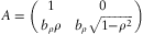$$$ A\: = \left( {\matrix{1 &amp; 0 \cr {b_\rho}\rho &amp; {{{b}_\rho }\sqrt {1{\rm{ - }}{{\rho }^2} } } }}\right) $$$, we obtain

$$\gamma _{{{{e}_1}}}^{ \ast } \left( {\widetilde{X}} \right)\: = \:\gamma _{{{{e}_2}}}^{ \ast } \left( {\widetilde{X}} \right)\: = \:1.$$

Moreover, analogously to (15), we obtain that

$${{(\gamma _{\xi }^{ \ast } (\widetilde{X}))}^{1/\alpha }} \: = \:{{\left( {{{{\left&#x007C; {{{\xi }^{(1)}} \: + \:{{\xi }^{(2)}} {{b}_\rho }\rho } \right&#x007C;}}^\alpha } \: + \:{{{\left&#x007C; {{{\xi }^{(2)}} {{b}_\rho }\sqrt {1{\rm{ - }}{{\rho }^2} } } \right&#x007C;}}^\alpha } } \right)}^{1/\alpha }} .$$

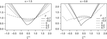
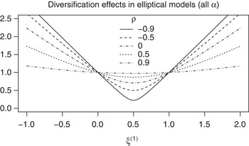
Figure 6 shows plots of $$$ {{(\gamma _{\xi }^{ \ast } (\tilde{X}))}^{1/\alpha }} $$$ for different α and ρ. The portfolio set also includes some short positions: ξ ⁽¹⁾ ranges in (−1, 2), and ξ ⁽²⁾ = 1−ξ ⁽¹⁾. The corresponding plot for the elliptical model is shown in Figure 7.

Figure 6

Asymptotic VaR ratio $$$ \gamma {{_{\xi }^{ \ast } }^{1/\alpha }} $$$ in the linear model $$$ \tilde{X}\: = \:\tilde{A}Y $$$ with balanced tails (short positions included).

Figure 7

Asymptotic VaR ratio $$$ \gamma {{_{\xi }^{ \ast } }^{1/\alpha }} $$$ in the elliptical model (short positions included).

First of all, we see that uniform ordering of portfolio risks is only possible for ξ∈Σ^d, i.e., if short positions are excluded. Furthermore, the re-weighting of X ⁽²⁾ to $$$ {{\tilde{X}}^{(2)}} $$$ shows that the linear t model with ρ ≥ 0 exhibits inversion of diversification effects for α < 1 in the same way as it would be in the pure loss case. If, however, ρ < 0, then there is no inversion of this kind, but also no uniform ordering of portfolio risks even for ξ ∈ Σ².

Moreover, the right part of Figure 6 shows that the downward pinnacles of the portfolio risk we saw in Figure 5 also appear for ρ > 0. However, in this case they are associated with short positions. These pinnacles correspond to the optimal hedging strategies that would minimize the asymptotic portfolio risk. It is clear that in case of positive dependence, hedging needs a negative portfolio weight. There are no such effects in the elliptical model.

This comparison shows that in case of compensation between losses and gains, asymptotic sub- and superadditivity of VaR for α < 1 is strongly influenced by the dependence structure. In particular, there is no general sub- or superadditivity result. Models that appear similar at a first glance can exhibit very different features. There seems to be a tendency of positive dependence to cause superadditivity. However, in models more complex than the linear model discussed here one would typically find a mixture of positive and negative dependence with an unclear outcome.