1. Introduction
Constitutive models for the fluid–particle drag force are widely utilized in the analysis of fluidized suspensions of solid particles (Sundaresan Reference Sundaresan2000). In fluidized beds, the buoyant weight of particles is principally balanced by the drag force exerted by the flowing fluid. As a result, the quantitative accuracy of model predictions depends critically on the accuracy of drag force models. Therefore, in order to achieve quantitative precision in the study of fluidized beds, such as those used in the pharmaceuticals or oil industries, it is vital to accurately model the drag force at the particle-scale level. Despite this fact, there are a number of limitations to the drag models that are currently available in the literature, one of which is the inability to account for the effect of particle translation and rotation. This particular limitation is addressed and remedied through the current work.
Models for the fluid–particle drag force have arisen through analytical (Brinkman Reference Brinkman1947; Kim & Russel Reference Kim and Russel1985; Koch & Sangani Reference Koch and Sangani1999), experimental (Darcy Reference Darcy1856; Kozeny Reference Kozeny1927; Carman Reference Carman1937; Ergun Reference Ergun1952; Richardson & Zaki Reference Richardson and Zaki1954; Wen & Yu Reference Wen and Yu1966; Garside & Al-Dibouni Reference Garside and Al-Dibouni1977; Davis & Acrivos Reference Davis and Acrivos1985; Gidaspow Reference Gidaspow1994; Nguyen & Ladd Reference Nguyen and Ladd2005) and computational methods (Hill, Koch & Ladd Reference Hill, Koch and Ladd2001; van der Hoef, Beetstra & Kuipers Reference van der Hoef, Beetstra and Kuipers2005; Beetstra, van der Hoef & Kuipers Reference Beetstra, van der Hoef and Kuipers2007; Tenneti, Garg & Subramaniam Reference Tenneti, Garg and Subramaniam2011). These drag relations seek to account for the interactions between fluid and particles over a range of particle volume fraction,
 ${\it\phi}$
, and Reynolds number,
 $Re$
. For a fluid–particle system, the particle volume fraction,
 ${\it\phi}$
, is defined as
 $$\begin{eqnarray}{\it\phi}=\frac{NV_{p}}{V_{tot}},\end{eqnarray}$$
where
 $V_{p}$
is the particle volume, and
 $N$
is the number of particles in the system of interest with volume
 $V_{tot}$
, while the Reynolds number is defined as
 $$\begin{eqnarray}Re=\frac{{\it\rho}_{f}(1-{\it\phi})|\boldsymbol{u}_{s}|d_{p}}{{\it\mu}_{f}},\end{eqnarray}$$
where
 ${\it\rho}_{f}$
is the fluid density,
 ${\it\mu}_{f}$
is the dynamic fluid viscosity,
 $d_{p}$
is diameter of the particle and
 $\boldsymbol{u}_{s}$
is the slip velocity, which is the difference between the fluid velocity,
 $\boldsymbol{u}_{f}$
, and the particle velocity,
 $\boldsymbol{v}_{p}$
. Constitutive relations for the fluid–particle drag force are often cast in terms of a dimensionless drag force,
 $F$
, which is defined as
 $$\begin{eqnarray}F=\frac{\boldsymbol{f}_{fp}\boldsymbol{\cdot }\boldsymbol{u}_{s}}{\boldsymbol{F}_{d,\mathit{Stokes}}\boldsymbol{\cdot }\boldsymbol{u}_{s}},\end{eqnarray}$$
where
 $\boldsymbol{f}_{fp}$
is the total fluid–particle interaction force minus the generalized buoyancy arising from the slowly varying stress field, and the Stokes drag relation on a single spherical particle at infinite dilution in a viscous fluid is given by
 $$\begin{eqnarray}\boldsymbol{F}_{d,\mathit{Stokes}}=3{\rm\pi}{\it\mu}_{f}d_{p}\boldsymbol{u}_{s}.\end{eqnarray}$$
Thus, the quantity
 $F$
can be thought of as a quantitative measure of the deviation from the ideal Stokes behaviour (
 ${\it\phi}\rightarrow 0$
and
 $Re\rightarrow 0$
).
In the literature, two of the more commonly employed fluid–particle drag relations are the models of Wen & Yu (Reference Wen and Yu1966) and Beetstra et al. (Reference Beetstra, van der Hoef and Kuipers2007). In drag studies like that of Beetstra et al. (Reference Beetstra, van der Hoef and Kuipers2007), highly resolved numerical simulations based on the lattice Boltzmann method (LBM) are used to study the flow of fluid past a fixed bed of solid particles. On the other hand, drag relations, like that of Wen & Yu (Reference Wen and Yu1966), are developed from sedimentation experiments. At the low-
 $Re$
limit, the drag relation of Beetstra et al. (Reference Beetstra, van der Hoef and Kuipers2007) as a function of
 ${\it\phi}$
is given by the model of van der Hoef et al. (Reference van der Hoef, Beetstra and Kuipers2005):
 $$\begin{eqnarray}F_{\mathit{van\,der\,Hoef}}({\it\phi})=\frac{10{\it\phi}}{1-{\it\phi}}+(1-{\it\phi})^{3}(1+1.5\sqrt{{\it\phi}}),\end{eqnarray}$$
while the equation of Wen & Yu (Reference Wen and Yu1966) is given by
 $$\begin{eqnarray}F_{Wen{-}Yu}=(1-{\it\phi})^{-(n-2)},\end{eqnarray}$$
with
 $n=4.65$
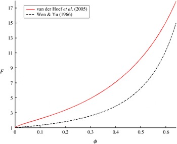
(Wen & Yu Reference Wen and Yu1966). In figure 1, the dimensionless drag curves of Wen & Yu (Reference Wen and Yu1966) and van der Hoef et al. (Reference van der Hoef, Beetstra and Kuipers2005) as functions of
 ${\it\phi}$
are compared. Key similarities between these two drag curves are that
 $F\rightarrow 1$
as
 ${\it\phi}\rightarrow 0$
, and
 $F$
increases monotonically as
 ${\it\phi}$
increases. In the low-
 $Re$
regime, the dimensionless drag of van der Hoef et al. (Reference van der Hoef, Beetstra and Kuipers2005) is significantly greater than the drag of Wen & Yu (Reference Wen and Yu1966) over the entire range of
 ${\it\phi}$
. The critical distinction between these two types of fluid–particle systems is that in the case of van der Hoef et al. (Reference van der Hoef, Beetstra and Kuipers2005), the particles are fixed in place and therefore unable to rotate and translate, while in the case of Wen & Yu (Reference Wen and Yu1966), the rotational and translational velocities of the particles are able to quickly adapt to the effects of the surrounding flow, which allows the fluid to move through with less drag. The Stokes number,
 $St$
, which is defined as
 $$\begin{eqnarray}St=\frac{{\it\rho}_{p}(1-{\it\phi})|\boldsymbol{u}_{s}|d_{p}}{18{\it\mu}_{f}}=\frac{{\it\rho}_{p}}{{\it\rho}_{f}}\frac{Re}{18},\end{eqnarray}$$
where
 ${\it\rho}_{p}$
is the particle density, can be used to characterize this distinction. Here
 $St$
is the ratio of the particle relaxation time to the fluid relaxation time, and so it is a critical parameter for quantifying the resistance of the particles to changes in their translational and rotational velocities due to the surrounding fluid flow. From this definition, the fixed bed (in the case of van der Hoef et al. (Reference van der Hoef, Beetstra and Kuipers2005)) represents the high-
 $St$
limit of fluidized systems, while the sedimentation of solid particles in liquid (in the case of Wen & Yu (Reference Wen and Yu1966)) represents the low-
 $St$
limit behaviour.
The dimensionless drag force,
 $F$
, as a function of the particle volume fraction,
 ${\it\phi}$
, is plotted for both the model of van der Hoef et al. (Reference van der Hoef, Beetstra and Kuipers2005) (low-
 $Re$
limit of the model of Beetstra et al. (Reference Beetstra, van der Hoef and Kuipers2007)) and that of Wen & Yu (Reference Wen and Yu1966) at the low-
 $Re$
limit. From this figure, it is clear that
 $F_{\mathit{van\,der\,Hoef}}>F_{Wen{-}Yu}$
over the entire range of
 ${\it\phi}$
.

Even though the drag models of Wen & Yu (Reference Wen and Yu1966) and Beetstra et al. (Reference Beetstra, van der Hoef and Kuipers2007) are derived from starkly different flow conditions and have significantly different values (figure 1), they are often applied interchangeably. In the work of Igci & Sundaresan (Reference Igci and Sundaresan2011) and Ozel, Fede & Simonin (Reference Ozel, Fede and Simonin2013), the model of Wen & Yu (Reference Wen and Yu1966) is used as the drag closure for the large-scale simulations of a gas–solid fluidized bed, while in similar studies, Pepiot & Desjardins (Reference Pepiot and Desjardins2012) and Radl & Sundaresan (Reference Radl and Sundaresan2014) instead employ the model of Beetstra et al. (Reference Beetstra, van der Hoef and Kuipers2007). Thus, there is a great deal of ambiguity in the fluidization literature about the applicability of the different drag models, particularly in terms of the different
 $St$
limits. Li & Kuipers (Reference Li and Kuipers2003) found that the predicted flow behaviour of a fluidized bed can be very sensitive to the form of the fluid–particle drag force, and so achieving precision in large-scale modelling of fluidized beds relies heavily on using drag relations that are truly applicable to the system of interest.
The current work looks to determine a drag model that is applicable to low-
 $Re$
fluidized systems over a full range of
 $St$
and
 ${\it\phi}$
. Towards this goal, LBM simulations are employed, in which, unlike the majority of prior LBM drag studies, the particles are allowed to freely translate and rotate based on the effects of the surrounding fluid. In doing so, the effects of particle translation and rotation are accounted for in a drag relation that bridges the transition from the low-
 $St$
regime (Wen & Yu (Reference Wen and Yu1966) type model) to the high-
 $St$
regime (van der Hoef et al. (Reference van der Hoef, Beetstra and Kuipers2005) or Beetstra et al. (Reference Beetstra, van der Hoef and Kuipers2007) model). Due to the fact that the drag model derived from the current work is valid over the entire range of
 $St$
and
 ${\it\phi}$
, its application to larger-scale simulation studies of fluidized beds will result in greater quantitative precision.
In § 2, we summarize the simulation method. In § 3, we present the simulation results and provide the equation for the drag model that accounts for both
 $St$
and
 ${\it\phi}$
in the low-
 $Re$
regime. Finally, in § 4, we provide some concluding remarks on the overall findings of this work.
2. Simulation method
2.1. Numerical set-up for the LBM scheme
In LBM, the fluid flow is simulated by the movement of fluid parcels along a three-dimensional lattice of nodes (Benzi, Succi & Vergassola Reference Benzi, Succi and Vergassola1992). The movement from one node to its neighbour is governed by the Boltzmann equation, which is discretized in both time and space. It can be demonstrated that the equations that describe the fluid dynamics obey the incompressible Navier–Stokes equations in the low-Mach-number limit (Chen & Doolen Reference Chen and Doolen1998; Aidun & Clausen Reference Aidun and Clausen2010). LBM, which dates back to the work of McNamara & Zanetti (Reference McNamara and Zanetti1988), was first employed in the study of fluid flows in the works of Higuera & Jimenez (Reference Higuera and Jimenez1989), Higuera & Succi (Reference Higuera and Succi1989) and Higuera, Succi & Benzi (Reference Higuera, Succi and Benzi1989). The scheme used in this study for the evolution of the fluid density and momentum distributions is described by Somers (Reference Somers1993) and Eggels & Somers (Reference Eggels and Somers1995). This implementation is a slight variant of the widely used LBGK scheme (Qian, d’Humieres & Lallemand Reference Qian, d’Humieres and Lallemand1992), with a more stable behaviour at low viscosities and second-order accuracy in space and time. LBM was first used to study the interaction between fluid and solid particles by Ladd (Reference Ladd1994). In the current scheme, the no-slip condition at the boundaries between the fluid and particles is handled with a forcing scheme, which is similar to the immersed boundary method (Goldstein, Handler & Sirovich Reference Goldstein, Handler and Sirovich1993; Derksen & van den Akker Reference Derksen and van den Akker1999; ten Cate et al.
Reference ten Cate, Nieuwstad, Derksen and van den Akker2002). This type of method for resolving the fluid–particle boundary, which utilizes an internal fluid, is stable for values of
 ${\it\rho}_{p}/{\it\rho}_{f}$
that are sufficiently larger than one (ten Cate et al.
Reference ten Cate, Nieuwstad, Derksen and van den Akker2002). In this forcing scheme, additional forces are imposed on the fluid at the surface of the solid sphere, such that the fluid velocity matches the local velocity of the solid surface. The force and torque that the fluid exerts on a solid particle are then computed by summing over these local forces that are needed to maintain a no-slip condition at the particle’s surface.
There are a number of subgrid particle–particle interaction forces that are explicitly included in the LBM scheme. As two particles approach each other, the accuracy of the LBM breaks down due to a lack of spatial resolution in the gap between the particles (Ladd Reference Ladd1997). An additional particle–particle lubrication force is therefore introduced in order to account for the contributions of the unresolved part of the flow field (Kim & Karilla Reference Kim and Karilla1991; Nguyen & Ladd Reference Nguyen and Ladd2002). Further details of the numerical scheme used in our study can be found in the work of Derksen & Sundaresan (Reference Derksen and Sundaresan2007).
In order to facilitate the computational scheme for modelling the particle–particle collisions, the particles are assigned a degree of softness. This softness is characterized by a collision time,
 $t_{c}$
, between two particles. The Hookean spring constant,
 $k$
, for the elastic collisions is defined as
 $$\begin{eqnarray}k=\frac{{\rm\pi}^{3}{\it\rho}_{p}d_{p}^{3}}{6t_{c}^{2}}.\end{eqnarray}$$
A particle–particle interaction force therefore arises due to these soft collisions. In this work, the collision between particles is assumed to be elastic and frictionless. For all of the simulations in the current study,
 $t_{c}$
is taken to be 10 LBM time steps, which corresponds to a maximum particle–particle overlap of about
 $0.001d_{p}$
. The total force and torque acting on each particle are then used in the equations of motion to update each particle’s velocity and position.
Spherical monodisperse particles are used in the current LBM simulations. The input diameter, in units of lattice spacing, is specified for the particles. Because the spherical particle is defined over a cubic grid, the effective hydrodynamic diameter of the spherical particle,
 $d_{p}$
, differs slightly from the input diameter. A calibration procedure, based on the work of Ladd (Reference Ladd1994), is used to determine
 $d_{p}$
from the input diameter and kinematic viscosity,
 ${\it\nu}_{f}$
, of the fluid. Larger values of
 $d_{p}$
correspond to a more fully resolved fluid flow profile and thus a finer grid resolution.
Throughout the current study, fully periodic boundary conditions in all three dimensions are employed. Furthermore, a body force is applied to both the particles and fluid in order to drive flow in the system, as described by Derksen & Sundaresan (Reference Derksen and Sundaresan2007). This body force can be interpreted as the superposition of a downward gravity force and an upward pressure gradient. In this periodic system, the strength of the pressure gradient is set such that the total body force on the fluid and particles is zero. Since
 ${\it\rho}_{p}>{\it\rho}_{f}$
, the net body force on the particles is downward, while the net body force on the fluid is upward. Since the lattice units are dimensionless, the lattice spacing,
 ${\it\Delta}$
, and the time step are simply taken to be 1. For a given simulation system, the key parameters that need to be provided are
 $d_{p}$
,
 ${\it\nu}_{f}$
, the particle-to-fluid density ratio,
 ${\it\rho}_{p}/{\it\rho}_{f}$
, the strength of the applied external body force,
 $f_{ext}$
, the total number of particles,
 $N$
, and the dimensions of the lattice,
 $n_{x}$
,
 $n_{y}$
and
 $n_{z}$
. Additionally, the initial coordinates of each of the particles are provided. From (1.1), the domain-averaged particle volume fraction,
 $\overline{{\it\phi}}$
, is determined from
 $N$
,
 $d_{p}$
and the system dimensions. For a typical simulation in the current study,
 $d_{p}$
is taken to be
 $12$
,
 ${\it\nu}_{f}$
is taken to be
 $0.1$
and
 $n_{x}$
,
 $n_{y}$
and
 $n_{z}$
are all taken to be
 $6d_{p}$
. A study of the sensitivity of the observed fluid–particle dynamics to changes in the grid resolution is provided in § 3.2.2. Furthermore,
 $f_{ext}$
and
 ${\it\rho}_{p}/{\it\rho}_{f}$
are both varied over a range of values, such that the flow remains in the low-
 $Re$
regime but a large range of
 $St$
is sampled. It is important to note that because
 $Re$
and
 $St$
are both functions of
 $\boldsymbol{u}_{s}$
, they are not set a priori. Instead, these parameters are determined from the results of the simulations.
In this study, we also investigated the characteristics of systems at the two limits of
 $St$
: a high-
 $St$
limit bed (fixed bed) and a low-
 $St$
limit bed. The additional constraints that must be applied to simulations of high-
 $St$
and low-
 $St$
limit beds are discussed in the following section.
2.2. Simulating high- and low-
 $St$
limit cases

In order to gain a more complete understanding of the behaviour of fluidized beds at the two
 $St$
limits, high and low, we look to simulate these two cases using the LBM scheme. However, in order to simulate the proper dynamics of these two limiting cases, additional constraints are necessary. These constraints are ascertained by analysing the effect of
 $Re$
and
 $St$
on the governing equations of motion.
The equation of motion for the position of a single particle is given as
 $$\begin{eqnarray}\frac{\text{d}\boldsymbol{x}_{p}}{\text{d}t}=\boldsymbol{v}_{p},\end{eqnarray}$$
where
 $\boldsymbol{x}_{p}$
is the position of the particle. In a fluidized suspension, the linear momentum balance for a spherical particle is given by
 $$\begin{eqnarray}{\it\rho}_{p}\frac{{\rm\pi}}{6}d_{p}^{3}\frac{\text{d}\boldsymbol{v}_{p}}{\text{d}t}=({\it\rho}_{p}-\overline{{\it\rho}})\frac{{\rm\pi}}{6}d_{p}^{3}\boldsymbol{g}+\boldsymbol{f}_{fp},\end{eqnarray}$$
where
 $\overline{{\it\rho}}=\overline{{\it\phi}}{\it\rho}_{p}+(1-\overline{{\it\phi}}){\it\rho}_{f}$
is the mixture density and
 $\boldsymbol{g}$
is the gravitational acceleration vector. Other forces, like particle–particle contact, which are included in the LBM simulations, can be added to the right-hand side of (2.3), but for the purposes of simplifying the current analysis, they are not included. Furthermore, the angular momentum balance for the spherical particle is given by
 $$\begin{eqnarray}{\it\rho}_{p}\frac{{\rm\pi}}{60}d_{p}^{5}\frac{\text{d}{\it\bf\Omega}_{p}}{\text{d}t}=\boldsymbol{T},\end{eqnarray}$$
where
 ${\it\bf\Omega}_{p}$
is the angular velocity of the particle and
 $\boldsymbol{T}$
is the torque of the fluid acting on the particle.
The equations of motion for the fluid phase are given as
 $$\begin{eqnarray}\displaystyle & \displaystyle \frac{\partial ({\it\rho}_{f}(1-{\it\phi}))}{\partial t}+\boldsymbol{{\rm\nabla}}\boldsymbol{\cdot }({\it\rho}_{f}(1-{\it\phi})\boldsymbol{u}_{f})=\mathbf{0}, & \displaystyle\end{eqnarray}$$
 $$\begin{eqnarray}\displaystyle & \displaystyle \frac{\text{D}_{f}}{\text{D}t}({\it\rho}_{f}(1-{\it\phi})\boldsymbol{u}_{f})=-(1-{\it\phi})\boldsymbol{{\rm\nabla}}p^{\prime }+(1-{\it\phi})({\it\rho}_{f}-\overline{{\it\rho}})\boldsymbol{g}-(1-{\it\phi})\boldsymbol{{\rm\nabla}}\boldsymbol{\cdot }{\bf\tau}_{f}-\frac{6}{{\rm\pi}}\frac{{\it\phi}}{d_{p}^{3}}\boldsymbol{f}_{fp}, & \displaystyle \nonumber\\ \displaystyle & & \displaystyle\end{eqnarray}$$
 ${\bf\tau}_{f}$
is the deviatoric fluid stress tensor and
 $\text{D}_{f}/\text{D}t$
is the total fluid material derivative with respect to time.
 $\boldsymbol{{\rm\nabla}}p^{\prime }$
is the rapidly varying pressure gradient term, where the total pressure gradient,
 $\boldsymbol{{\rm\nabla}}p$
, is given by
 $\boldsymbol{{\rm\nabla}}p=\overline{{\it\rho}}\boldsymbol{g}+\boldsymbol{{\rm\nabla}}p^{\prime }$
. At the surface of each particle, no-slip and no-penetration boundary conditions are imposed.
Using a scaling analysis, in which we look to retain all of the contributions to the net force (right-hand side in (2.3) and (2.6)) and assume that
 ${\it\rho}_{f}$
does not vary, we obtain the following set of non-dimensional governing equations:
 $$\begin{eqnarray}\displaystyle & \displaystyle \frac{\text{d}\tilde{\boldsymbol{x}}_{p}}{\text{d}\tilde{t}}=\tilde{\boldsymbol{v}}_{p}, & \displaystyle\end{eqnarray}$$
 $$\begin{eqnarray}\displaystyle & \displaystyle St_{c}\frac{\text{d}\tilde{\boldsymbol{v}}_{p}}{\text{d}\tilde{t}}=\tilde{\boldsymbol{g}}+\tilde{\boldsymbol{f}}_{fp}, & \displaystyle\end{eqnarray}$$
 $$\begin{eqnarray}\displaystyle & \displaystyle St_{c}\frac{\text{d}\tilde{{\it\bf\Omega}}_{p}}{\text{d}\tilde{t}}=\widetilde{\boldsymbol{T}}. & \displaystyle\end{eqnarray}$$
 $$\begin{eqnarray}\displaystyle & \displaystyle \frac{\partial (1-{\it\phi})}{\partial \tilde{t}}+\tilde{\boldsymbol{{\rm\nabla}}}\boldsymbol{\cdot }((1-{\it\phi})\tilde{\boldsymbol{u}}_{f})=\mathbf{0}, & \displaystyle\end{eqnarray}$$
 $$\begin{eqnarray}\displaystyle & \displaystyle \!\!Re_{c}\frac{\text{D}_{f}}{\text{D}\tilde{t}}((1-{\it\phi})\tilde{\boldsymbol{u}}_{f})=-(1-{\it\phi})\tilde{\boldsymbol{{\rm\nabla}}}\tilde{p}^{\prime }-18\!\left(\frac{\overline{{\it\rho}}-{\it\rho}_{f}}{{\it\rho}_{p}-\overline{{\it\rho}}}\right)\!(1-{\it\phi})\tilde{\boldsymbol{g}}-(1-{\it\phi})\tilde{\boldsymbol{{\rm\nabla}}}\boldsymbol{\cdot }\tilde{{\bf\tau}}_{f}-18{\it\phi}\tilde{\boldsymbol{f}}_{fp}, & \displaystyle \nonumber\\ \displaystyle & & \displaystyle\end{eqnarray}$$
 $\tilde{\boldsymbol{x}}_{p}=\boldsymbol{x}_{p}/d_{p}$
,
 $\tilde{\boldsymbol{v}}_{p}=\boldsymbol{v}_{p}/u_{c}$
,
 $\tilde{t}=t/(d_{p}/u_{c})$
,
 $\tilde{\boldsymbol{g}}=\boldsymbol{g}/g$
,
 $\tilde{\boldsymbol{f}}_{fp}=\boldsymbol{f}_{fp}/(3{\rm\pi}d_{p}{\it\mu}_{f}u_{c})$
,
 $\tilde{{\it\bf\Omega}}_{p}={\it\bf\Omega}_{p}/(u_{c}/d_{p})$
,
 $\widetilde{\boldsymbol{T}}=\boldsymbol{T}/(3{\rm\pi}d_{p}^{2}{\it\mu}_{f}u_{c}/10)$
,
 $\tilde{\boldsymbol{{\rm\nabla}}}=d_{p}\boldsymbol{{\rm\nabla}}$
,
 $\tilde{\boldsymbol{u}}_{f}=\boldsymbol{u}_{f}/u_{c}$
,
 $\tilde{p}^{\prime }=p^{\prime }/({\it\mu}_{f}u_{c}/d_{p})$
and
 $\tilde{{\bf\tau}}_{f}={\bf\tau}_{f}/({\it\mu}_{f}u_{c}/d_{p})$
. In these expressions, the characteristic superficial slip velocity is
 $u_{c}=(1-{\it\phi}_{c})|\boldsymbol{u}_{s,c}|$
, where the subscript
 $c$
denotes a characteristic quantity, and
 $g=|\boldsymbol{g}|$
. Furthermore, the characteristic Stokes number,
 $St_{c}$
, and characteristic Reynolds number,
 $Re_{c}$
, are given by
 $$\begin{eqnarray}\displaystyle & \displaystyle St_{c}=\frac{{\it\rho}_{p}u_{c}d_{p}}{18{\it\mu}_{f}}, & \displaystyle\end{eqnarray}$$
 $$\begin{eqnarray}\displaystyle & \displaystyle Re_{c}=\frac{{\it\rho}_{f}u_{c}d_{p}}{{\it\mu}_{f}}. & \displaystyle\end{eqnarray}$$
 $u_{c}$
is chosen such that the drag force balances the force of gravity and the effects of the imposed pressure gradient on a single particle at infinite dilution:
 $$\begin{eqnarray}u_{c}=\frac{({\it\rho}_{p}-\overline{{\it\rho}})d_{p}^{2}g}{18{\it\mu}_{f}}.\end{eqnarray}$$
From this non-dimensionalization, the effect of
 $St$
and
 $Re$
on the equations governing particles and fluid can be ascertained.
Focusing on the left-hand side of (2.7)–(2.11), it is observed that
 $Re$
multiplies the term
 $(\text{D}_{f}/\text{D}\tilde{t})((1-{\it\phi})\tilde{\boldsymbol{u}}_{f})$
,
 $St$
multiplies the terms
 $\text{d}\tilde{\boldsymbol{v}}_{p}/\text{d}\tilde{t}$
and
 $\text{d}\tilde{{\it\bf\Omega}}_{p}/\text{d}\tilde{t}$
, and the term
 $\text{d}\tilde{\boldsymbol{x}}_{p}/\text{d}\tilde{t}$
is multiplied by 1. The high- and low-
 $St$
limit cases are then cast in terms of these dimensionless groups:
 $Re$
,
 $St$
and 1. Since the current study focuses on the low-
 $Re$
regime,
 $Re\ll 1$
. Thus, in the high-
 $St$
limit,
 $Re\ll 1\ll St$
, and so the particle velocities (both linear and angular) evolve over a much longer time than do the particle positions, which, in turn, evolve over a much longer time than does the fluid velocity. Thus, the fluid velocity field is in a quasisteady state (QSS) relative to the particle positions and velocities. In the low-
 $St$
limit,
 $Re,St\ll 1$
, and so the particle positions evolve over a much longer time than do the particle velocities and fluid velocity. The fluid and particle velocities, therefore, are in a QSS relative to the particle positions.
It is important to specify that
 $Re$
refers to the Reynolds number based on the mean slip velocity. We can express
 $\boldsymbol{v}_{p}$
and
 ${\it\bf\Omega}_{p}$
as
 $$\begin{eqnarray}\displaystyle \boldsymbol{v}_{p}=\langle \boldsymbol{v}_{p}\rangle +\boldsymbol{v}_{p}^{\prime }, & & \displaystyle\end{eqnarray}$$
 $$\begin{eqnarray}\displaystyle {\it\bf\Omega}_{p}=\langle {\it\bf\Omega}_{p}\rangle +{\it\bf\Omega}_{p}^{\prime }, & & \displaystyle\end{eqnarray}$$
 $\langle \boldsymbol{v}_{p}\rangle$
and
 $\langle {\it\bf\Omega}_{p}\rangle$
are the average linear and angular velocities, respectively, of all of the particles in the simulation region. We use
 $\boldsymbol{v}_{p}^{\prime }$
and
 ${\it\bf\Omega}_{p}^{\prime }$
to denote the corresponding fluctuations from the mean value. Since
 $\langle {\it\bf\Omega}_{p}\rangle =\mathbf{0}$
in our systems of interest, we can consider two additional Reynolds numbers based on the two fluctuation velocities:
 $$\begin{eqnarray}\displaystyle Re_{T}=\displaystyle \frac{{\it\rho}_{f}d_{p}}{{\it\mu}_{f}}\sqrt{\frac{1}{3}\langle \boldsymbol{v}_{p}^{\prime }\boldsymbol{\cdot }\boldsymbol{v}_{p}^{\prime }\rangle }, & & \displaystyle\end{eqnarray}$$
 $$\begin{eqnarray}\displaystyle Re_{{\it\Omega}}=\displaystyle \frac{{\it\rho}_{f}d_{p}^{2}}{{\it\mu}_{f}}\sqrt{\frac{1}{3}\langle {\it\bf\Omega}_{p}^{\prime }\boldsymbol{\cdot }{\it\bf\Omega}_{p}^{\prime }\rangle }, & & \displaystyle\end{eqnarray}$$
 $\langle \,\rangle$
is used to designate a quantity that is averaged over all of the particles in the system. In this study, we limit our attention to
 $Re_{T},Re_{{\it\Omega}},Re\ll 1$
. In gas–solid systems of moderate to high
 $Re$
, Wylie, Koch & Ladd (Reference Wylie, Koch and Ladd2003) and Kriebitzsch, van Der Hoef & Kuipers (Reference Kriebitzsch, van Der Hoef and Kuipers2013) demonstrated the significance of the effect of fluctuations in the velocities of the particles, quantified by the granular temperature, on the fluid–particle drag force. However, in low-
 $Re$
systems, these effects of granular temperature are found to be less pronounced. Furthermore, recent work by Zhou & Fan (Reference Zhou and Fan2014) has used LBM simulations to look at additional contributions to the fluid–particle interaction force besides the drag force, namely the Magnus lift force, which arises due to the effects of strong particle rotation. However, in the current study, the flow conditions are such that the drag force is the single dominant contribution to the overall interaction force. In these systems, the fluid–particle interaction forces that are perpendicular to the slip velocity, like the Magnus lift force, represent less than 1 % of the total interaction force.
2.2.1. High-
$St$
limit

At the high-
 $St$
limit (
 $Re\ll 1\ll St$
), the fluid relaxes very quickly compared with the particles, and so the fluid is in a QSS relative to the particles. In the reference frame where
 $\langle \boldsymbol{v}_{p}\rangle =\mathbf{0}$
, the high-
 $St$
fluidized system is characterized by a mean fluid velocity,
 $\langle \boldsymbol{u}_{f}\rangle$
,
 $\boldsymbol{v}_{p}^{\prime }$
and
 ${\it\bf\Omega}_{p}^{\prime }$
. Since
 $Re_{T},Re_{{\it\Omega}},Re\ll 1$
, this system can be interpreted as a linear superposition of the following three systems: (1) a fixed-bed system, in which there is a mean fluid velocity,
 $\langle \boldsymbol{u}_{f}\rangle$
, but
 $\boldsymbol{v}_{p}^{\prime }={\it\bf\Omega}_{p}^{\prime }=\mathbf{0}$
; (2) a system in which the particles have fluctuations in their linear velocities, but
 $\langle \boldsymbol{u}_{f}\rangle ={\it\bf\Omega}_{p}^{\prime }=\mathbf{0}$
; and (3) a system in which the particles have fluctuations in their angular velocities, but
 $\langle \boldsymbol{u}_{f}\rangle =\boldsymbol{v}_{p}^{\prime }=\mathbf{0}$
. Since there is no mean flow in systems (2) and (3), these systems do not contribute to the overall fluid–particle drag force. Thus, the drag force for the overall high-
 $St$
fluidized system arises solely from system (1). Thus, the high-
 $St$
limit case can be represented by a fixed-particle bed. In the LBM simulations of the high-
 $St$
limit case, the fluid moves around the fixed particles, and eventually a QSS flow distribution is established for a given particle configuration and external driving force. Since the particles do not translate or rotate in any way to adjust to the surrounding flow, the high-
 $St$
limit provides the upper limit for the dimensionless drag force,
 $F$
, in the low-
 $Re$
regime.
2.2.2. Low-
$St$
limit

At the low-
 $St$
limit (
 $Re,St\ll 1$
), the fluid and particle velocities are in a QSS relative to the particle positions. In this case, the velocities (linear and angular) of the particles evolve much faster than their positions, as the particles respond immediately to the flow. Lattice Boltzmann simulations, in which the particle positions are frozen, are used as a computational method for finding the QSS velocities of the particles and fluid. At each step in the simulations, the particle velocities are updated, as usual, based on the net forces and torques acting on each particle. The particle positions, on the other hand, are not changed. As these simulations converge to a steady state, the net force and torque on each particle approach zero. The computed equilibrium velocity profile provides the dynamics for a low-
 $St$
limit bed at a single instant in time. Since the linear and angular velocities of the particles adjust very quickly to the flow of the surrounding fluid, the low-
 $St$
limit provides the lower limit for
 $F$
in a low-
 $Re$
fluidized bed.
3. Simulation results
3.1. High-
$St$
limit with a random array of particles

The high-
 $St$
limiting behaviour is established by simulating a fixed-particle bed, as motivated in § 2.2.1. It is understood that all of the relevant Reynolds numbers are small, leaving
 $St$
and
 ${\it\phi}$
as the only dimensionless quantities of interest for the present study. For each simulation, the particles are arranged in a random, homogeneous configuration. To obtain each random configuration, the particles are thermalized using a discrete element method (DEM) simulation. This thermalization method places particles in the DEM simulation box at random, assigning each particle a random velocity from a Gaussian distribution. The particles are then allowed to move around and collide without the effects of the fluid or gravity. After each particle has undergone many collisions, a snapshot of the DEM simulation is taken. The random, homogeneous configuration of particles for the LBM simulations is then obtained from this DEM snapshot. In this case and throughout the study, the dimensionless drag force,
 $F$
(1.3), is computed by averaging the fluid velocity, particle velocities and fluid–particle interaction forces over the entire domain (Euler–Euler approach). In these domain-averaged calculations, the values of
 ${\it\phi}$
and
 $\overline{{\it\phi}}$
are equivalent. The data that are used to compute
 $F$
for a fixed bed are taken from a snapshot of the system after the steady state has been reached. A particle diameter of
 $d_{p}=12$
and a kinematic fluid viscosity of
 ${\it\nu}_{f}=0.1$
are used for these simulations. These fixed-bed simulations are conducted over a wide range of
 ${\it\phi}$
values. For each value of
 ${\it\phi}$
, the results are averaged over a large number (between 10 and 60) of random, homogeneous particle configurations. Since the particle positions are held fixed and all of the simulations are conducted in the low-
 $Re$
regime, the high-
 $St$
drag results are independent of
 $f_{ext}$
and
 ${\it\rho}_{p}/{\it\rho}_{f}$
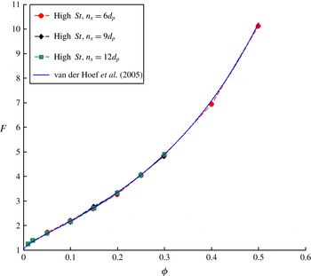
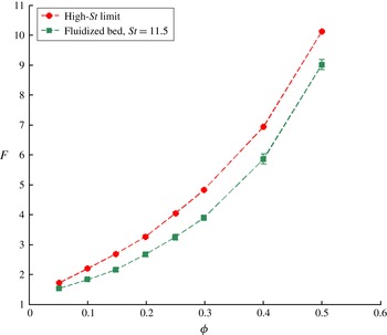
. In figure 2, the results for
 $F$
as a function of
 ${\it\phi}$
are presented for three different cubic periodic domain sizes:
 $n_{x}=6d_{p}$
,
 $9d_{p}$
and
 $12d_{p}$
. From figure 2, we see that the effect of the domain size on the high-
 $St$
limit case is negligible. Furthermore, from figure 2, we see that the high-
 $St$
limit drag curve matches very closely the drag curve (1.5) of van der Hoef et al. (Reference van der Hoef, Beetstra and Kuipers2005), which was also computed for fixed-particle systems. This result confirms the validity of the current LBM numerical scheme. This same set of parameters, with a cubic domain size of
 $n_{x}=6d_{p}$
and a grid resolution of
 $d_{p}=12$
and
 ${\it\nu}_{f}=0.1$
, is used for the majority of the current study.
The dimensionless drag force,
 $F$
, is computed over a range of domain-averaged particle volume fractions,
 ${\it\phi}$
, for a fixed-particle bed (high-
 $St$
limit), for three different cubic periodic domain sizes:
 $n_{x}=6d_{p}$
,
 $9d_{p}$
and
 $12d_{p}$
. The effects of the domain size appear to be negligible for the high-
 $St$
limit case. These drag curves match very closely the drag curve of van der Hoef et al. (Reference van der Hoef, Beetstra and Kuipers2005).

3.2. Simulations of fluidized beds
Relaxing the constraint that the particles have to be held fixed in place, we then look to study the dynamics of a fluidized bed, in which the particles are free to translate and rotate based on the forces and torques that act on them. For each fluidized bed simulation,
 $f_{ext}$
and
 ${\it\rho}_{p}/{\it\rho}_{f}$
are specified. The initial configuration of particles is random and homogeneous, and is obtained using a DEM thermalization technique. As time evolves, the particle positions change as particle structures and voids form in the system. The data that are used to compute
 $F$
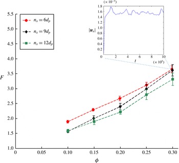
for a fluidized bed are taken from snapshots of the system after a statistical steady state has been reached. At each of these snapshots in time, taken from simulations of fluidized beds, we extract the particle positions, fluid and particle velocities, as well as the fluid–particle interaction forces. The criterion for determining the statistical steady state is based on the time evolution of the domain-averaged slip velocity (as shown in the inset to figure 3). Due to the mobility of the particles, the slip velocity does not approach a single steady-state value, as in the fixed-bed simulations, so the statistical steady state is based on the time-averaged slip velocity approaching a constant value. As in the high-
 $St$
limit case, an Euler–Euler averaging approach is used for determining the values of
 $F$
. For each set of
 ${\it\rho}_{p}/{\it\rho}_{f}$
,
 $f_{ext}$
and
 ${\it\phi}$
, the value of
 $F$
is determined by averaging over the results of 10 different initial particle configurations. Since
 $St$
is a function of the slip velocity, it is determined, like
 $F$
, by averaging over the results of the different initial particle configurations.
3.2.1. Effect of domain size on the dynamics of fluidized beds
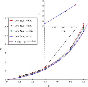
In figure 3, the results for
 $F$
over a range of
 ${\it\phi}$
for a
 $St=11.5$
fluidized bed are presented for three different cubic periodic domain sizes:
 $n_{x}=6d_{p}$
,
 $9d_{p}$
and
 $12d_{p}$
. The value of
 $f_{ext}$
is set such that
 $Re$
is of the order of 0.1, and properly adjusted in order to achieve the desired value of
 $St$
, which we show in § 3.6 is the key parameter for the current study. From figure 3, over the entire range of
 ${\it\phi}$
, there is a significant decrease in
 $F$
as the domain size,
 $n_{x}$
, increases. Due to the mobility of particles in the fluidized case, as the domain size increases, the length scale over which particle structures form increases, which leads to an increase in the extent of flow-induced inhomogeneities in the distribution of particles. Increases in the extent of inhomogeneities lead to the formation of larger voids in the system. The fluid is able to preferentially move through these larger voids, leading to a smaller overall fluid–particle drag force, thus explaining the reduction in
 $F$
as
 $n_{x}$
increases. While there is a clear effect of domain size on the drag results for a fluidized bed, the current study looks to draw conclusions about the effect of particle translation and rotation on the fluid–particle drag force that are applicable to essentially homogeneous systems. Thus, we focus on studying the dynamics of fluidized beds with a cubic periodic domain size of
 $n_{x}=6d_{p}$
, and then look to form conclusions that can be extended to homogeneous systems.
 $F$
is computed over a range of domain-averaged particle volume fractions,
 ${\it\phi}$
, for a
 $St=11.5$
fluidized bed for three different cubic periodic domain sizes:
 $n_{x}=6d_{p}$
,
 $9d_{p}$
and
 $12d_{p}$
. For all of these cases,
 $d_{p}=12$
and
 ${\it\nu}_{f}=0.1$
. As
 $n_{x}$
increases, there is a decrease in the value of
 $F$
. This drag reduction is due to an increase in the extent of inhomogeneities in the particle configuration that comes from increases in the domain size. In the inset to this figure, the magnitude of the fluid–particle slip velocity,
 $|\boldsymbol{u}_{s}|$
, is plotted as a function of time for the case of
 ${\it\phi}=0.3$
,
 $n_{x}=6d_{p}$
. This type of plot is used to determine when the fluidized bed has reached a statistical steady state.

3.2.2. Effect of grid resolution on the dynamics of fluidized beds
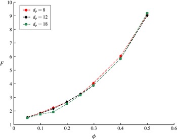
In order to assess the sensitivity of the simulation dynamics of the fluidized bed to changes in the grid resolution, the drag curve is determined for a fluidized bed for several different grid resolutions. Keeping
 ${\it\nu}_{f}$
fixed at a value of 0.1, the effect of grid resolution on the fluid–particle drag force is assessed by analysing systems with three different particle diameters:
 $d_{p}=8$
, 12 and 18. The results of this grid resolution study are shown in figure 4, where
 $F$
is plotted as a function of
 ${\it\phi}$
for a
 $St=11.5$
fluidized bed. From figure 4, we observe that there is a very small difference in drag between the
 $d_{p}=12$
and
 $d_{p}=18$
cases. Thus, we conclude from this grid sensitivity analysis that a value of
 $d_{p}=12$
provides a sufficient amount of resolution. System parameters of
 $d_{p}=12$
and
 ${\it\nu}_{f}=0.1$
are used for the remainder of this study.
 $F$
is computed over a range of domain-averaged particle volume fractions,
 ${\it\phi}$
, for a
 $St=11.5$
fluidized bed for three different grid resolutions (or particle diameters):
 $d_{p}=8$
, 12 and 18. For all of these cases,
 ${\it\nu}_{f}=0.1$
. From this grid sensitivity analysis, a small difference between the
 $d_{p}=12$
and
 $d_{p}=18$
drag curves is observed. Therefore, a value of
 $d_{p}=12$
is taken to provide a sufficient amount of grid resolution for the current study.

3.2.3. Comparison of the drag curve for the high-
$St$
limit and fluidized beds

In figure 5, the results for
 $F$
as a function of
 ${\it\phi}$
for a
 $St=11.5$
fluidized bed are compared with the high-
 $St$
limit (fixed-particle bed) drag values. From figure 5, the drag values for the
 $St=11.5$
fluidized bed are clearly smaller than those for the high-
 $St$
limit case. This drag reduction in the fluidized bed relative to the fixed bed is due to a combination of two factors: the ability of the particles to translate and rotate due to the effects of the surrounding fluid, and the development of inhomogeneities in the particle configuration. Through this work, we look to better understand each of these effects on the drag force.
The drag values,
 $F$
, over a range of
 ${\it\phi}$
are compared for a
 $St=11.5$
fluidized bed and a high-
 $St$
limit (fixed-particle) bed. For both sets of simulations, the following set of parameters are used:
 $d_{p}=12$
,
 ${\it\nu}_{f}=0.1$
and
 $n_{x}=6d_{p}$
. It is found that there is a drag reduction going from the high-
 $St$
limit curve to the fluidized bed curve.

3.3. Effect of particle translation and rotation: high-
$St$
versus low-
$St$
limit


The extent to which the particles are able to translate and rotate in response to the effects of the surrounding fluid decreases as
 $St$
increases. As discussed in § 3.1, the fixed-particle bed represents the high-
 $St$
limit case. At the other extreme is the low-
 $St$
limit case, for which the linear and angular velocities of the particles evolve much faster than the particle positions, as discussed in § 2.2.2. The drag curve for the low-
 $St$
limit case is determined using simulations, in which the configuration of particles is random, homogeneous and static. In order to ensure that there is no bias from the particle configurations when comparing the results of the low-
 $St$
limit with those of the high-
 $St$
limit, the same random configurations that were obtained using DEM simulations for the high-
 $St$
limit case are used for the low-
 $St$
limit case. Like the high-
 $St$
simulations, the low-
 $St$
simulations are conducted over a wide range of
 ${\it\phi}$
values. For each value of
 ${\it\phi}$
, the results are averaged over a large number (between 10 and 60) of random, homogeneous particle configurations. Since the particles are held at their initial positions and all of the simulations are conducted in the low-
 $Re$
regime, the low-
 $St$
drag results are independent of
 $f_{ext}$
and
 ${\it\rho}_{p}/{\it\rho}_{f}$
.
3.3.1. Effect of domain size on the low-
$St$
limit simulations

We start by analysing the effect of the domain size on the fluid–particle drag in the low-
 $St$
limit case. In figure 6, the results for
 $F$
as a function of
 ${\it\phi}$
are presented for three different cubic periodic domain sizes:
 $n_{x}=6d_{p}$
,
 $9d_{p}$
and
 $12d_{p}$
. From figure 6, there is a clear reduction in drag in the low-
 $St$
limit case as the domain size increases. In contrast to the fluidized bed case, as an equilibrium velocity profile is established in the low-
 $St$
limit simulations, the development of flow-induced inhomogeneities is suppressed by keeping the particles fixed in place. Thus, the effects of periodicity (or domain size) can be eliminated by extrapolating the low-
 $St$
limit drag results to an infinite domain size. Using a
 $1/n_{x}$
dependence, as shown in the inset of figure 6 for the
 ${\it\phi}=0.3$
case, the drag results are extrapolated to an infinite domain size
 $(n_{x}\rightarrow \infty )$
. While the drag curve given by (1.6) has a constant exponent,
 $n$
, the
 $n_{x}\rightarrow \infty$
drag results are best fitted with an exponent that varies with
 ${\it\phi}$
:
 $n({\it\phi})=6.2-2.5{\it\phi}$
. Outside the dilute limit, this value of
 $n$
primarily lies in the range 4.65–5.5 given by the sedimentation experiments of Richardson & Zaki (Reference Richardson and Zaki1954), Wen & Yu (Reference Wen and Yu1966) and Garside & Al-Dibouni (Reference Garside and Al-Dibouni1977). Furthermore, this drag curve has a similar form to the analytical approximation of Brady & Durlofsky (Reference Brady and Durlofsky1988) for the hindered sedimentation velocity. Such a result confirms that the low-
 $St$
limit simulations indeed provide an accurate depiction of the fluid–particle interactions in liquid–solid sedimentation.
 $F$
is computed over a range of domain-averaged particle volume fractions,
 ${\it\phi}$
, for a low-
 $St$
limit bed for three different cubic periodic domain sizes:
 $n_{x}=6d_{p}$
,
 $9d_{p}$
and
 $12d_{p}$
. System parameters of
 $d_{p}=12$
and
 ${\it\nu}_{f}=0.1$
are used for all of these simulations. Using a
 $1/n_{x}$
dependence, these results are extrapolated to an infinite domain size
 $(n_{x}\rightarrow \infty )$
, as shown in the inset for the case
 ${\it\phi}=0.3$
. The drag curve for the
 $n_{x}\rightarrow \infty$
low-
 $St$
limit matches very closely the drag curve (1.6) of Wen & Yu (Reference Wen and Yu1966) type, with a
 ${\it\phi}$
-dependent exponent:
 $n({\it\phi})=6.2-2.5{\it\phi}$
.

3.3.2. High-
$St$
limit versus low-
$St$
limit


As discussed in § 3.2.1, our goal is to form conclusions about the dynamics of fluid–particle interactions that can be extended to nearly homogeneous systems by using periodic simulation cells of domain size
 $n_{x}=6d_{p}$
. Towards this goal, we compare the high-
 $St$
and low-
 $St$
drag curves using results obtained from simulation cells of domain size
 $n_{x}=6d_{p}$
. These results for
 $F$
as a function of
 ${\it\phi}$
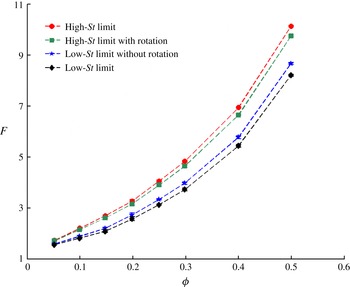
are shown in figure 7, where we observe a significant reduction in drag when moving from the high-
 $St$
limit curve to the low-
 $St$
limit curve. This drag reduction ranges from 10 % for
 ${\it\phi}=0.05$
to 19 % for
 ${\it\phi}=0.5$
. Since the high- and low-
 $St$
limit cases are both simulated using identical random, homogeneous particle configurations, this drag reduction is not a result of changes in the extent of inhomogeneities. Instead, this drag reduction is due to the evolution of the linear and angular velocities of the particles in response to the effects of the surrounding fluid in the low-
 $St$
limit case. Since the low-
 $St$
limit particles are able to adapt to the fluid velocity field, there is less fluid–particle drag in the low-
 $St$
limit case when compared with the high-
 $St$
limit case, where the particles are not able to adjust at all to the effects of the surrounding fluid. From this analysis, we conclude that for any given particle configuration in the low-
 $Re$
regime, the high-
 $St$
limit case maximizes the fluid–particle drag in the system, while the low-
 $St$
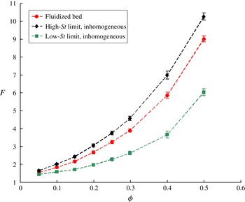
limit case minimizes the drag. Figure 7 is analogous to figure 1 where the curve of van der Hoef et al. (Reference van der Hoef, Beetstra and Kuipers2005) is compared with that of Wen & Yu (Reference Wen and Yu1966).
 $F$
as a function of
 ${\it\phi}$
is compared for (1) the high-
 $St$
limit case, (2) the high-
 $St$
limit case with particle rotation, (3) the low
 $St$
limit case without particle rotation and (4) the low-
 $St$
limit case. The results for all of these cases are taken from periodic cells with a domain size of
 $n_{x}=6d_{p}$
. In order to ensure that there is no bias due to the configuration of particles, all four cases use the same random, homogeneous particle configurations. It is clear that the low-
 $St$
limit case has the lowest drag over the entire range of
 ${\it\phi}$
. This drag reduction on moving from the high-
 $St$
limit to the low-
 $St$
limit is due to the evolution of the linear and angular velocities of the low-
 $St$
limit particles in response to the fluid velocity field.

In figure 7, the drag results for two additional hypothetical cases are shown: high-
 $St$
limit with particle rotation (to achieve zero net torque) and low-
 $St$
limit without particle rotation. Due to the ability of the particles to rotate in response to the surrounding fluid in the case of the high-
 $St$
limit with rotation, there is a small reduction in drag when compared with the case of the regular high-
 $St$
limit. This drag reduction ranges from 1 % for
 ${\it\phi}=0.05$
to 4 % for
 ${\it\phi}=0.5$
. Furthermore, when the particles are not allowed to rotate in the low-
 $St$
limit, there is a small increase in drag when compared with the case of the regular low-
 $St$
limit. This increase in drag ranges from 2 % for
 ${\it\phi}=0.05$
to 6 % for
 ${\it\phi}=0.5$
. Thus, the difference in
 $F$
between the high-
 $St$
and low-
 $St$
limits is mostly due to the ability of the particles in the latter case to attain non-zero translational velocity in order to achieve zero net force. In the Appendix, further details of the impact of particle velocity fluctuations on drag are given. It is demonstrated there that in the low-
 $St$
limit, the fluctuations are coherent and lead to a reduction of drag as compared to fixed beds (i.e. the high-
 $St$
limit). It is also shown that random, uncorrelated velocity fluctuations do not induce a drag-reducing effect.
3.4. Effect of flow-induced inhomogeneities
In order to assess the importance of flow-induced inhomogeneities on the fluid–particle drag, we isolate the effects of inhomogeneities from that of particle translation and rotation by simulating high- and low-
 $St$
limit beds using what we refer to as ‘frozen’ fluidized particle configurations. These ‘frozen’ configurations are obtained by taking a snapshot from a fluidized bed simulation long after a statistical steady state has been reached. Due to the formation of particle clusters and voids in the fluidized beds, these ‘frozen’ configurations are inhomogeneous. High-
 $St$
and low-
 $St$
limit simulations are then conducted using these inhomogeneous configurations. The same set of inhomogeneous configurations are used for both the high- and low-
 $St$
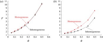
limit cases. In figure 8, the results of
 $F$
over a range of
 ${\it\phi}$
for the inhomogeneous high-
 $St$
(figure 8
a) and low-
 $St$
(figure 8
b) limit cases are compared with their respective values taken from random, homogeneous configurations. The inhomogeneous configurations are taken from fluidized beds with
 $St=11.5$
. In the high-
 $St$
limit case (figure 8
a), when moving from the homogeneous curve to the inhomogeneous curve, there is a small but noticeable reduction in drag at lower particle volume fractions
 $({\it\phi}<0.3)$
, and no change in drag as the packing fraction approaches the close packing limit
 $({\it\phi}>0.3)$
. From these results, the development of inhomogeneities appears to be hindered at higher particle volume fractions. In the low-
 $St$
limit case (figure 8
b), when moving from the homogeneous curve to the inhomogeneous curve, there is a significant reduction in drag over the entire range of
 ${\it\phi}$
. Thus, it appears that inhomogeneities in the particle configuration have a stronger effect on the fluid–particle drag when the particle velocities are able to adjust to the effects of the surrounding fluid. Overall, inhomogeneities have a noticeable effect on the fluid–particle interactions, and must therefore be accounted for when devising a drag model.
The values of
 $F$
over a range of
 ${\it\phi}$
taken from the ‘frozen’, inhomogeneous fluidized configurations are compared with values taken from a random, homogeneous configuration for both (a) the high-
 $St$
limit case and (b) the low-
 $St$
limit case. The inhomogeneous configurations are obtained by taking snapshots of
 $St=11.5$
fluidized beds long after a statistical steady state has been achieved. In the high-
 $St$
limit case, when moving from the homogeneous curve to the inhomogeneous curve, there is a small reduction in drag in the range
 ${\it\phi}<0.3$
, and no effect on the drag in the range
 ${\it\phi}>0.3$
. In the low-
 $St$
limit case, the inhomogeneous drag curve is significantly lower than the homogeneous curve over the entire range of
 ${\it\phi}$
. Overall, the effects of inhomogeneities tend to result in a drag reduction.

The goal of this study is to obtain a drag model that can be applied to larger-scale numerical studies of fluidized beds. For studies of this type, the drag relations are typically applied at length scales over which the particle configuration is taken to be approximately homogeneous. Therefore, we seek to obtain a drag relation that is applicable to fluidized beds with homogeneous particle configurations. To achieve this goal, we need to isolate the effects of particle translation and rotation from the effects of inhomogeneities.
3.5. Quantification of relative fluidized bed behaviour
In order to isolate the effect of particle translation and rotation from the effect of inhomogeneities, we compare the dimensionless drag curves taken from the following three systems: (1)
 $St=St_{given}$
fluidized bed, (2) the high-
 $St$
limit bed that uses the inhomogeneous configuration of particles taken from snapshots of the
 $St_{given}$
fluidized bed, and (3) the low-
 $St$
limit bed that uses the inhomogeneous configuration of particles also taken from the
 $St_{given}$
fluidized bed. In doing so, we are comparing these three different types of systems by taking drag data from snapshots that contain identical configurations of particles. Thus, the observed differences in the drag values are solely a result of the differences in the abilities of the particles to translate and rotate. In figure 9, these three drag curves are shown for particle configurations taken from
 $St=11.5$
fluidized bed simulations. We see that, as expected, the high-
 $St$
limit case maximizes the drag, while the low-
 $St$
limit case minimizes the drag for any given configuration. The drag for the fluidized bed lies in between these two limits over the full range of
 ${\it\phi}$
.
The drag values,
 $F$
, as a function of
 ${\it\phi}$
are shown for three different system types: (1) the
 $St=11.5$
fluidized bed, (2) the high-
 $St$
limit bed using inhomogeneous particle configurations taken from snapshots of the
 $St=11.5$
fluidized bed, and (3) the low-
 $St$
limit using inhomogeneous particle configurations taken from snapshots of the
 $St=11.5$
fluidized bed. There is a reduction in drag going from the high-
 $St$
limit case to the fluidized bed case to the low-
 $St$
limit case due to the effects of particle translation and rotation.

The relative behaviour of the fluidized bed compared with the high- and low-
 $St$
limit cases is quantified using the ratio
 ${\it\alpha}$
, which we define as
 $$\begin{eqnarray}{\it\alpha}=\frac{F_{\mathit{fluidized}}-F_{\mathit{low\,St,\,inhom}}}{F_{\mathit{high\,St,\,inhom}}-F_{\mathit{low\,St,\,inhom}}}.\end{eqnarray}$$
Since the high- and low-
 $St$
limit cases provide the two limiting values for the drag,
 $0\leqslant {\it\alpha}\leqslant 1$
. For a fluidized bed exhibiting low-
 $St$
limit behaviour,
 ${\it\alpha}=0$
, and for a fluidized bed exhibiting high-
 $St$
limit behaviour,
 ${\it\alpha}=1$
.
3.6. Using
${\it\alpha}$
to define a new drag model

Using the method shown in figure 9 and (3.1),
 ${\it\alpha}$
is computed over a range of
 ${\it\phi}$
,
 ${\it\rho}_{p}/{\it\rho}_{f}$
,
 $Re$
and
 $St$
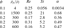
. A sample of these results is presented in table 1. From the first two rows of data in table 1, it is clear that when two different systems have the same
 ${\it\phi}$
and
 $Re$
, but have a different
 ${\it\rho}_{p}/{\it\rho}_{f}$
, the value of
 ${\it\alpha}$
is different. Furthermore, by comparing the third and fourth rows of table 1, it is clear that when two different systems have the same
 ${\it\phi}$
and
 ${\it\rho}_{p}/{\it\rho}_{f}$
, but have different values of
 $Re$
, the value of
 ${\it\alpha}$
is different. Finally, by comparing the fourth and fifth rows of data in table 1, it appears that when two different systems have the same
 ${\it\phi}$
and
 $St$
, but different values of
 ${\it\rho}_{p}/{\it\rho}_{f}$
and
 $Re$
, the value
 ${\it\alpha}$
is nearly the same. Thus,
 ${\it\alpha}={\it\alpha}({\it\phi},St)$
.
The results for
 ${\it\alpha}$
for several different types of fluidized beds.

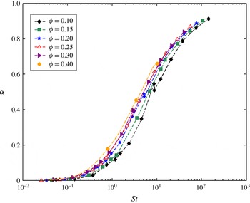
In figure 10,
 ${\it\alpha}$
is plotted as a function of
 $St$
for domain-averaged particle volume fractions,
 ${\it\phi}$
, ranging from 0.1 to 0.4. For each curve of
 ${\it\alpha}$
versus
 $St$
, three distinct regimes are observed: (1) the low-
 $St$
regime, where
 ${\it\alpha}\rightarrow 0$
as
 $St\rightarrow 0$
; (2) the intermediate-
 $St$
regime, where there is a gradual increase in
 ${\it\alpha}$
as
 $St$
increases; and (3) the high-
 $St$
regime, where
 ${\it\alpha}\rightarrow 1$
as
 $St\rightarrow \infty$
. Thus, we see that
 ${\it\alpha}$
describes the transition from the low-
 $St$
regime to the high-
 $St$
regime. As
 ${\it\phi}$
increases, the transition from the low-
 $St$
regime to the high-
 $St$
regime occurs at lower values of
 $St$
. The reason for this is that at higher values of
 ${\it\phi}$
, the fluidized bed tends to behave more like a packed bed, and so the transition to a high-
 $St$
limit type of behaviour occurs at lower values of
 $St$
.
 ${\it\alpha}$
is plotted as a function of
 $St$
over a wide range of
 ${\it\phi}$
. The simulation results are taken from a periodic domain size of
 $n_{x}=6d_{p}$
. For each value of
 ${\it\phi}$
, three distinct regimes are observed: (1) the low-
 $St$
regime (
 ${\it\alpha}\rightarrow 0$
as
 $St\rightarrow 0$
), (2) intermediate-
 $St$
regime (
 ${\it\alpha}$
gradually increases as
 $St$
increases) and (3) high-
 $St$
regime (
 ${\it\alpha}\rightarrow 1$
as
 $St\rightarrow \infty$
). Furthermore, as
 ${\it\phi}$
increases, the fluidized bed tends to behave more like a packed bed, and so the transition to a high-
 $St$
limit type of behaviour occurs at lower values of
 $St$
.

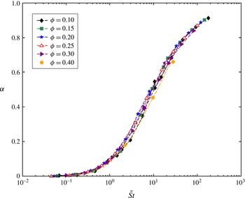
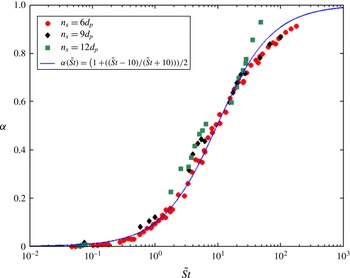
Analysing the results of figure 10, we see that we can collapse the curves of
 ${\it\alpha}$
versus
 $St$
onto a single curve by using a modified Stokes number,
 $\tilde{St}$
, which is defined as
 $$\begin{eqnarray}\tilde{St}=\frac{St}{(1-{\it\phi})^{2}},\end{eqnarray}$$
with
 $St$
defined as in (1.7). The results of
 ${\it\alpha}$
as a function of
 $\tilde{St}$
for a wide range of
 ${\it\phi}$
are shown in figure 11. The exponent of 2 in (3.2) provides the most complete collapse of the
 ${\it\alpha}$
versus
 $St$
data onto a single curve, and seems to capture the effect of higher packing fractions hindering the free translation and rotation of particles, causing the flow to transition to the high-
 $St$
limit at lower values of
 $St$
for more packed-bed-like cases (higher values of
 ${\it\phi}$
). Thus, for a domain size of
 $n_{x}=6d_{p}$
,
 ${\it\alpha}$
is solely a function of
 $\tilde{St}$
.
 ${\it\alpha}$
is plotted as a function of
 $\tilde{St}$
over a wide range of
 ${\it\phi}$
values. The choice of
 $\tilde{St}=St/(1-{\it\phi})^{2}$
allows all of the
 ${\it\alpha}$
curves to collapse onto a single curve. For a domain size of
 $n_{x}=6d_{p}$
,
 ${\it\alpha}$
is solely a function of
 $\tilde{St}$
.

3.6.1. Effect of domain size on
${\it\alpha}$

The effect of the domain size on
 ${\it\alpha}$
as a function of
 $\tilde{St}$
is shown in figure 12. In figure 12, we see that even as the system size is changed from
 $n_{x}=6d_{p}$
to
 $n_{x}=9d_{p}$
to
 $n_{x}=12d_{p}$
, the curve of
 ${\it\alpha}$
as a function of
 $\tilde{St}$
remains approximately unchanged. As the size of the system size increases, the extent to which the particles are able to form structures increases, and so the extent of inhomogeneities increases. Despite the fact that the domain size of our periodic system has an effect on the development of flow structures and on the distribution of particles, we have developed a method for characterizing the extent to which particles are able to translate and rotate that is independent of the domain size. Thus, we have found that
 ${\it\alpha}(\tilde{St})$
is applicable to nearly homogeneous systems. A simple curve that follows the shape of
 ${\it\alpha}(\tilde{St})$
is given by
 $$\begin{eqnarray}{\it\alpha}(\tilde{St})=\frac{1}{2}\left(1+\frac{\tilde{St}-10}{\tilde{St}+10}\right).\end{eqnarray}$$
The form of (3.3) appears to suggest that
 $\tilde{St}=10$
is the centre point for the intermediate-
 $St$
regime. For
 $\tilde{St}<1$
, the fluid–particle system is in the low-
 $St$
regime, while for
 $\tilde{St}>100$
, the system is in the high-
 $St$
regime.
 ${\it\alpha}$
is plotted as a function of
 $\tilde{St}$
for domain sizes of
 $6d_{p}$
,
 $9d_{p}$
and
 $12d_{p}$
. From this curve, we see that
 ${\it\alpha}(\tilde{St})$
does not vary significantly with the domain size. A single fitted curve is then used to describe this
 ${\it\alpha}(\tilde{St})$
curve. The results shown in this plot are taken from a large range of
 ${\it\phi}$
.

From figure 12, we see that with the use of this
 ${\it\alpha}$
analysis, we have successfully formed conclusions about the fluid–particle interactions that are applicable to nearly homogeneous systems. We have observed a dependence of
 $\tilde{St}$
on the fluid–particle drag force, primarily using simulation systems with a domain size of
 $n_{x}=6d_{p}$
, that remains valid even as the domain size changes. Such conclusions are particularly powerful in that they allow us to study the dynamics of the fluid–particle interactions with the use of a relatively small number of particles.
As discussed in § 3.4, the goal of this study is to obtain a constitutive relation for the fluid–particle drag force that is applicable to larger-scale simulations of fluid–particle systems. In these larger-scale simulations, the particle configuration is typically taken to be approximately homogeneous at the scale of the fluid grid size, and so we seek a drag model that is applicable to homogeneous configurations, which we denote as
 $F_{\mathit{fluidized,hom}}$
. Because
 ${\it\alpha}(\tilde{St})$
does not vary with
 $n_{x}$
, we can extrapolate the results to a system where the particle configuration is homogeneous:
 $$\begin{eqnarray}{\it\alpha}(\tilde{St})=\frac{F_{\mathit{fluidized}}-F_{\mathit{low\,St,\,inhom}}}{F_{\mathit{high\,St,\,inhom}}-F_{\mathit{low\,St,\,inhom}}}=\frac{F_{\mathit{fluidized,hom}}-F_{\mathit{low\,St,\,hom}}}{F_{\mathit{high\,St,\,hom}}-F_{\mathit{low\,St,\,hom}}}.\end{eqnarray}$$
Rearranging the terms in (3.4), we find that in the low-
 $Re$
regime, the drag relation, which is applicable to homogeneous particle distributions, is given by
 $$\begin{eqnarray}F({\it\phi},St)=F_{\mathit{fluidized,hom}}={\it\alpha}(\tilde{St})F_{\mathit{high\,St,\,hom}}({\it\phi})+(1-{\it\alpha}(\tilde{St}))F_{\mathit{low\,St,\,hom}}({\it\phi}).\end{eqnarray}$$
Since, in the low-
 $Re$
regime,
 $F_{\mathit{high\,St,\,hom}}=F_{\mathit{van\,der\,Hoef}}$
and
 $F_{\mathit{low\,St,\,hom}}=(1-{\it\phi})^{-(n({\it\phi})-2)}$
, (3.5) can be re-expressed as
 $$\begin{eqnarray}F({\it\phi},St)={\it\alpha}(\tilde{St})F_{\mathit{van\,der\,Hoef}}({\it\phi})+(1-{\it\alpha}(\tilde{St}))(1-{\it\phi})^{-(n({\it\phi})-2)},\end{eqnarray}$$
where
 ${\it\alpha}(\tilde{St})$
is given by (3.3),
 $F_{\mathit{van\,der\,Hoef}}({\it\phi})$
is given by (1.5) and
 $n({\it\phi})=6.2-2.5{\it\phi}$
, as shown in figure 6. In (3.6), we have proposed a new drag model, which is dependent on both
 ${\it\phi}$
and
 $St$
.
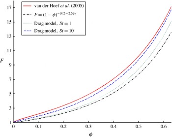
As shown in figure 13, the new drag relation is able to bridge the gap between the low-
 $St$
type models, like that of Wen & Yu (Reference Wen and Yu1966), and the high-
 $St$
type models, like that of van der Hoef et al. (Reference van der Hoef, Beetstra and Kuipers2005), and is applicable over a full range of
 $St$
in the low-
 $Re$
regime. This bridging property of the proposed drag model represents a significant improvement on prior drag relations, because this new model is able to more fully capture the effect of particle mobility on the fluid–particle interactions. In figure 13, the proposed drag model is shown for both
 $St=1$
and
 $St=10$
with
 $F$
as a function of
 ${\it\phi}$
. As expected, the
 $St=10$
drag is higher than the
 $St=1$
drag. When comparing these curves with the curve of van der Hoef et al. (Reference van der Hoef, Beetstra and Kuipers2005) and a drag curve of Wen & Yu (Reference Wen and Yu1966) type,
 $F=(1-{\it\phi})^{-(n-2)}$
with
 $n({\it\phi})=6.2-2.5{\it\phi}$
, we see that there is a significant difference between the predictions given by the new drag relation and those given by traditional models (Wen & Yu Reference Wen and Yu1966; van der Hoef et al.
Reference van der Hoef, Beetstra and Kuipers2005) and hybrid models (Gidaspow Reference Gidaspow1994) that are simply equal to the curve of Wen & Yu (Reference Wen and Yu1966) type at low
 ${\it\phi}$
and equal to that of van der Hoef et al. (Reference van der Hoef, Beetstra and Kuipers2005) type at high
 ${\it\phi}$
. Thus, in the low-
 $Re$
regime, unlike prior drag models, the proposed drag model (3.6) is able to describe the fluid–particle drag force over a full range of
 $St$
and
 ${\it\phi}$
.
The proposed drag model (3.6) is shown with a plot of the dimensionless drag force,
 $F$
, as a function of
 ${\it\phi}$
, for both
 $St=1$
and
 $St=10$
. These drag curves are compared with the curve of van der Hoef et al. (Reference van der Hoef, Beetstra and Kuipers2005) and with the drag curve of Wen & Yu (Reference Wen and Yu1966) type,
 $F=(1-{\it\phi})^{-(n({\it\phi})-2)}$
, with
 $n({\it\phi})=6.2-2.5{\it\phi}$
.

4. Summary
Through this work, a new drag model (3.6) has been proposed that, unlike previous drag models, is a function of both
 ${\it\phi}$
and
 $St$
in the low-
 $Re$
regime. Prior LBM drag studies have developed models for the fluid–particle drag force that are valid over the entire range of
 ${\it\phi}$
, but are only applicable to high-
 $St$
systems. Furthermore, prior hybrid drag models, like that of Gidaspow (Reference Gidaspow1994), have blended fixed-bed (for high
 ${\it\phi}$
) and sedimentation (for low
 ${\it\phi}$
) drag models, but have implicitly assumed that fluid–particle systems exhibit high-
 $St$
behaviour at high
 ${\it\phi}$
and low-
 $St$
behaviour at low
 ${\it\phi}$
. We have found that such a simplification is not accurate over a full range of
 $St$
. In the current work, we have developed a drag model that provides a smooth blending of the packed-bed and sedimentation drag models over both
 ${\it\phi}$
and
 $St$
. This new drag model bridges the transition from low
 ${\it\phi}$
to high
 ${\it\phi}$
, as well as from low
 $St$
to high
 $St$
. By accounting for the effect of particle translation and rotation on the interactions between the fluid and particles, this
 $St$
-dependent drag relation is able to capture a wider range of fluid and particle properties than was previously attainable through the drag models available in the literature.
The current drag model is constructed using LBM simulations with a cubic periodic domain. For larger-scale simulations of fluid–particle systems, the fluid grid size is larger than the particle diameter, and so the fluid–particle drag force cannot simply be computed by summing the forces over the surface of the particle, as is done in the case of LBM. Instead, the fluid–particle drag force is determined from an input constitutive relation. Since the distribution of particles is typically taken to be approximately homogeneous at the fluid grid scale, the drag model derived in the current work must be applicable to the homogeneous configuration in order for it to be used as a constitutive relation in the larger-scale simulations. Using a combination of fluidized, fixed and low-
 $St$
limit bed simulations, the methodology for obtaining the drag relation is successfully extrapolated to a homogeneous system. Thus, a drag model that is applicable to homogeneous particle distributions is obtained.
In summary, we have presented a framework for developing drag laws based on
 ${\it\phi}$
and
 $St$
. While the current analysis is for low-
 $Re$
systems, this methodology can be extended to higher values of
 $Re$
. Through its application to larger-scale numerical models of fluidized beds, this new drag relation has the potential to increase the quantitative precision of these models, and thus widen our understanding of a range of industrial processes.
Acknowledgements
This work is supported by a grant from the ExxonMobil Research & Engineering Co., and by a fellowship awarded to G.J.R. by the National Science Foundation (DGE-1148900).
Appendix. Effect of velocity fluctuations in the low-
$Re$
regime

The validity of the low-
 $Re$
fixed-bed simulations is further probed by analysing the effect of fluctuations in the angular and linear particle velocities on the drag force. The strength of the fluctuations in
 $\boldsymbol{v}_{p}$
is characterized by
 $Re_{T}$
(2.17), while the strength of the fluctuations in
 ${\it\bf\Omega}_{p}$
is characterized by
 $Re_{{\it\Omega}}$
(2.18). In the homogeneous low-
 $St$
limit simulations, particles attain non-zero values of
 $\boldsymbol{v}_{p}$
and
 ${\it\bf\Omega}_{p}$
, such that the net force and torque on each particle are 0. In this low-
 $St$
limit case,
 $Re_{T}\approx 0.05$
and
 $Re_{{\it\Omega}}\approx 0.06$
. Although
 $Re$
,
 $Re_{T},Re_{{\it\Omega}}\ll 1$
in the low-
 $St$
limit case, there is a significant reduction (between 10 % and 20 %) in drag when compared with the case of a fixed bed (high-
 $St$
limit), as discussed in § 3.3.2. The reason for this drag reduction is that while the fluctuations in
 $\boldsymbol{v}_{p}$
and
 ${\it\bf\Omega}_{p}$
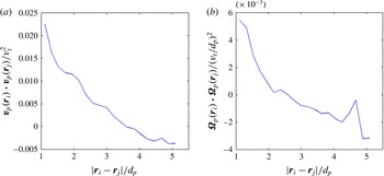
are small, they are not random. There is a clear correlation in the particle velocity fluctuations based on their locations within the flow, as shown in figure 14(a,b). These correlated velocity fluctuations in the low-
 $St$
limit case act to reduce the drag of the fluid flow past the homogeneous array of particles.
The correlations of fluctuations in (a)
 $\boldsymbol{v}_{p}$
and (b)
 ${\it\bf\Omega}_{p}$
in the low-
 $St$
limit case with particle separation distance are shown. In these plots, the subscripts
 $i$
and
 $j$
designate two different particles in the system, while
 $v_{t}$
is the terminal particle velocity and
 $\boldsymbol{r}_{i}$
is the position of particle
 $i$
. There is a clear positive correlation in both
 $\boldsymbol{v}_{p}$
and
 ${\it\bf\Omega}_{p}$
at small particle distances, which signifies that the velocity fluctuations in the low-
 $St$
limit case are not random.

Since
 $Re$
,
 $Re_{T},Re_{{\it\Omega}}\ll 1$
, the low-
 $St$
limit case with
 $f_{ext}$
and non-zero values of
 $\boldsymbol{v}_{p}=\boldsymbol{v}_{p,\,low\,St}$
and
 ${\it\bf\Omega}_{p}={\it\bf\Omega}_{p,\,low\,St}$
can be broken into a superposition of the following three systems: (1) a fixed bed with
 $f_{ext}$
, and zero
 $\boldsymbol{v}_{p}$
and
 ${\it\bf\Omega}_{p}$
; (2) a system with zero
 $f_{ext}$
and
 ${\it\bf\Omega}_{p}$
, and
 $\boldsymbol{v}_{p}=\boldsymbol{v}_{p,\,low\,St}$
; and (3) a system with zero
 $f_{ext}$
and
 $\boldsymbol{v}_{p}$
, and
 ${\it\bf\Omega}_{p}={\it\bf\Omega}_{p,\,low\,St}$
. By simulating each of these subsystems, we found that such a superposition is valid by confirming that
 $\boldsymbol{u}_{s,\,low\,St}=\boldsymbol{u}_{s,\,case\,1}+\boldsymbol{u}_{s,\,case\,2}+\boldsymbol{u}_{s,\,case\,3}$
. This result demonstrates that the fluctuations in
 $\boldsymbol{v}_{p}$
and
 ${\it\bf\Omega}_{p}$
in the low-
 $St$
limit case are indeed small. Furthermore, we observe that the small, correlated values of
 $\boldsymbol{v}_{p}$
and
 ${\it\bf\Omega}_{p}$
in cases (2) and (3), respectively, produce a mean flow (non-zero value of
 $\boldsymbol{u}_{s}$
) even in the absence of an external force,
 $f_{ext}$
.
Next, we look to investigate the effect of small, random fluctuations in
 $\boldsymbol{v}_{p}$
and
 ${\it\bf\Omega}_{p}$
, with intensities equivalent to that of the correlated fluctuations in the low-
 $St$
case:
 $Re_{T}\approx 0.05$
and
 $Re_{{\it\Omega}}\approx 0.06$
, respectively. We study these random fluctuations via the following four systems: (1) a system with
 $f_{ext}$
and random fluctuations in
 $\boldsymbol{v}_{p}$
; (2) a system with
 $f_{ext}$
and random fluctuations in
 ${\it\bf\Omega}_{p}$
; (3) a system with zero
 $f_{ext}$
and random fluctuations in
 $\boldsymbol{v}_{p}$
; and (4) a system with zero
 $f_{ext}$
and random fluctuations in
 ${\it\bf\Omega}_{p}$
. In each case, the velocity value imposed on each particle is chosen at random from a Gaussian distribution. We find that the dimensionless drag force,
 $F$
, for case (1) is nearly equivalent to that of the fixed bed. In fact, these drag values differ by just 0.02 % at
 ${\it\phi}=0.3$
and by 0.67 % at
 ${\it\phi}=0.25$
. Similarly, we find that the values of
 $F$
for case (2) are equivalent to within 0.1 % to that of the fixed bed. Since
 $Re$
,
 $Re_{T},Re_{{\it\Omega}}\ll 1$
in both of these cases, the contribution of the random fluctuations to the overall fluid–particle drag force is, as expected, negligible. Additionally, in simulating cases (3) and (4), we find that the small, random (uncorrelated) values of
 $\boldsymbol{v}_{p}$
and
 ${\it\bf\Omega}_{p}$
are unable to produce a mean flow in the absence of
 $f_{ext}$
. These sets of simulations further confirm the validity of the LBM scheme in the low-
 $Re$
regime.