1 Introduction
Instabilities in the wake of a long smooth bluff body subjected to steady incoming flow are among the most classical problems in fluid mechanics. It is well known that the flow is governed by a single dimensionless parameter, the Reynolds number
 $Re$
(
 $=UD/\unicode[STIX]{x1D708}$
), where
 $U$
is the approaching flow velocity,
 $D$
is the length scale of the cylinder perpendicular to the approaching flow and
 $\unicode[STIX]{x1D708}$
is the kinematic viscosity of the fluid. For a circular cylinder,
 $D$
is taken as the diameter of the cylinder. For a square cylinder which is oriented such that the front and rear sides of the cross-section are perpendicular to the approaching flow while the other two sides are parallel to the approaching flow (simply referred to as the square cylinder hereafter),
 $D$
is taken as the side length of the cylinder.
Three-dimensional (3-D) wake transition for flow past a circular cylinder has been studied extensively in the literature based on different methodologies, including physical model testing (e.g. Williamson Reference Williamson1996), linear (and nonlinear) stability analyses (e.g. Barkley & Henderson Reference Barkley and Henderson1996) and direct numerical simulation (DNS) (e.g. Henderson Reference Henderson1997; Jiang et al.
Reference Jiang, Cheng, Draper, An and Tong2016. Based on these investigations, it has been shown that with the increase of
 $Re$
the flow structure in the cylinder wake undergoes a transition sequence of: (i) emergence of a two-dimensional (2-D) primary wake instability at
 $Re\sim 47$
, (ii) onset of a Mode A (the first 3-D instability mode, with a spanwise wavelength of approximately
 $3.96D$
and an out-of-phase sequence between the neighbouring braids) instability with large-scale vortex dislocations (denoted as Mode A*) at
 $Re\sim 190$
, (iii) gradual wake transition from Mode A* to Mode B (the second 3-D instability mode, with a spanwise wavelength of approximately
 $0.82D$
and an in-phase sequence between the neighbouring braids) over a range of
 $Re$
from 230 to 260 and (iv) development of an increasingly disordered Mode B structure for
 $Re>$
270.
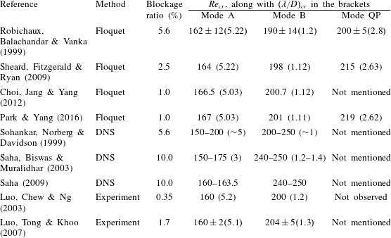
A number of studies are also available in the literature for the wake instabilities of a square cylinder. Three wake instability modes, i.e. Mode A, Mode B and a quasi-periodic Mode QP, have been discovered for flow past a square cylinder (Blackburn & Lopez Reference Blackburn and Lopez2003). Table 1 lists the critical Reynolds numbers
 $Re_{cr}$
and the corresponding spanwise wavelengths
 $(\unicode[STIX]{x1D706}/D)_{cr}$
for Modes A, B and QP predicted by various studies. It is seen that although Mode QP was discovered through Floquet stability analysis, it was not reported by DNS or experimental studies. This is consistent with the case of a circular cylinder.
The
 $Re_{cr}$
values and the corresponding spanwise wavelengths
 $(\unicode[STIX]{x1D706}/D)_{cr}$
for Modes A, B and QP predicted by various studies. The blockage ratio is defined as the side length of the cylinder to the cross-flow length of the computational domain or test section.

However, a consensus on the precise wake transition regimes for a square cylinder has not been reached. Scatters are observed in table 1 for the
 $Re_{cr}$
and
 $(\unicode[STIX]{x1D706}/D)_{cr}$
values, especially for the results obtained through DNS. Based on the results shown in table 1, the following questions are raised and remained to be answered:
-
(i) Theoretically speaking, the
 $Re_{cr}$
and
$(\unicode[STIX]{x1D706}/D)_{cr}$
values for Mode B predicted by physical experiments and DNS should be consistent. However, significant differences are observed in table 1. It is worthwhile seeking an answer for the observed discrepancy.
-
(ii) For flow past a circular cylinder, the onset point for Mode B instability obtained through physical experiments (e.g.
$Re=230$
by Williamson Reference Williamson1996) or DNS (e.g.
$Re=230$
by Jiang et al.
Reference Jiang, Cheng, Draper, An and Tong2016) is smaller than that predicted by Floquet stability analysis (e.g.
$Re=259$
by Barkley & Henderson Reference Barkley and Henderson1996). This is because the unstable 3-D modes discovered from Floquet stability analysis are based on the 2-D base flow, without taking into account the nonlinear interactions between the unstable modes (Henderson Reference Henderson1997). Whereas in reality, the existence of Mode A* flow would destabilize the braid shear layer region to allow for an early development of Mode B (Jiang et al.
Reference Jiang, Cheng, Draper, An and Tong2016). However, this trend is not observed for the case of a square cylinder (table 1). The
$Re_{cr}$
values for Mode B reported by Saha et al. (Reference Saha, Biswas and Muralidhar2003) and Saha (Reference Saha2009) through DNS are even much higher than the stability analysis results of
$Re_{cr}\sim 200$
. This challenges the explanation of the destabilization effect for Mode B proposed based on the case of a circular cylinder and warrants a further investigation.


Similar to the case of flow past a circular cylinder, the regular Mode A structure in the wake of a square cylinder would also evolve spontaneously into a more stable pattern with large-scale vortex dislocations, i.e. Mode A* (Luo et al.
Reference Luo, Chew and Ng2003; Saha et al.
Reference Saha, Biswas and Muralidhar2003), provided that the Mode A structure is not confined by a short spanwise size of the cylinder. In contrast to a sudden drop of the Strouhal number (
 $St$
) in the
 $St{-}Re$
relationship at the onset of Mode A* for the case of a circular cylinder (Williamson Reference Williamson1996), a gradual reduction of
 $St$
at the onset of Mode A* was reported by Luo et al. (Reference Luo, Chew and Ng2003) for a square cylinder. In a follow-up study by Luo et al. (Reference Luo, Tong and Khoo2007), however, a sudden drop rather than a gradual reduction of
 $St$
was observed at the onset of Mode A*.
For the wake transition process from Mode A* to Mode B, a single and continuous
 $St{-}Re$
curve was observed by Luo et al. (Reference Luo, Chew and Ng2003), whereas a discontinuous
 $St{-}Re$
curve and correspondingly twin-peaked vortex shedding frequency spectra (as is the case for flow past a circular cylinder, see, e.g. Williamson Reference Williamson1996) were reported by Luo et al. (Reference Luo, Tong and Khoo2007). Luo et al. (Reference Luo, Tong and Khoo2007) broadly attributed the difference between Luo et al. (Reference Luo, Chew and Ng2003) and Luo et al. (Reference Luo, Tong and Khoo2007) to the difference in the experimental set-ups.
In addition to physical experiments, DNS is also a useful tool in investigating the wake transition from Mode A* to Mode B, including the co-existence and interaction of the wake instability modes. However, since previous DNS studies were carried out with relatively large
 $Re$
intervals (e.g.
 $\unicode[STIX]{x0394}Re=50$
in Sohankar et al. (Reference Sohankar, Norberg and Davidson1999) and
 $\unicode[STIX]{x0394}Re=25$
in Saha et al. (Reference Saha, Biswas and Muralidhar2003)), a detailed wake transition process from Mode A* to Mode B or the gradual/sudden variations of the
 $St{-}Re$
curve, including at the onset of Mode A* and during the wake transition process from Mode A* to Mode B, could not be properly explored.
In light of the earlier works, the primary aim of this study is to investigate the wake transition for flow past a square cylinder through detailed DNS, with a particular focus on the mode interactions over the wake transition process from Mode A* to Mode B and the characteristics of the
 $St{-}Re$
relationship. In addition, major differences between wake transition of a square cylinder and a circular cylinder will be discussed.
2 Numerical model
2.1 Numerical method
OpenFOAM (www.openfoam.org) has been adopted in this study for solving the continuity and incompressible Navier–Stokes equations:
 $$\begin{eqnarray}\displaystyle & \displaystyle \frac{\unicode[STIX]{x2202}u_{i}}{\unicode[STIX]{x2202}x_{i}}=0 & \displaystyle\end{eqnarray}$$
 $$\begin{eqnarray}\displaystyle & \displaystyle \frac{\unicode[STIX]{x2202}u_{i}}{\unicode[STIX]{x2202}t}+u_{j}\frac{\unicode[STIX]{x2202}u_{i}}{\unicode[STIX]{x2202}x_{j}}=-\frac{1}{\unicode[STIX]{x1D70C}}\frac{\unicode[STIX]{x2202}p}{\unicode[STIX]{x2202}x_{i}}+\unicode[STIX]{x1D708}\frac{\unicode[STIX]{x2202}^{2}u_{i}}{\unicode[STIX]{x2202}x_{j}\unicode[STIX]{x2202}x_{j}}, & \displaystyle\end{eqnarray}$$
where
 $(x_{1},x_{2},x_{3})=(x,y,z)$
are Cartesian coordinates,
 $u_{i}$
is the velocity component in the direction
 $x_{i}$
,
 $t$
is time,
 $\unicode[STIX]{x1D70C}$
is fluid density,
 $p$
is pressure and
 $\unicode[STIX]{x1D708}$
is kinematic viscosity. The finite volume method (FVM) and the pressure implicit with splitting of operators (PISO) algorithm (Issa Reference Issa1986) are used to solve the equations. The convection, diffusion and time derivative terms are discretized, respectively, using a fourth-order cubic scheme, a second-order linear scheme and a blended scheme consisting of the second-order Crank–Nicolson scheme and a first-order Euler implicit scheme, respectively. The same numerical approach has been used in Jiang et al. (Reference Jiang, Cheng, Draper, An and Tong2016) for the simulations of wake transition of a circular cylinder.
2.2 Computational domain and boundary conditions
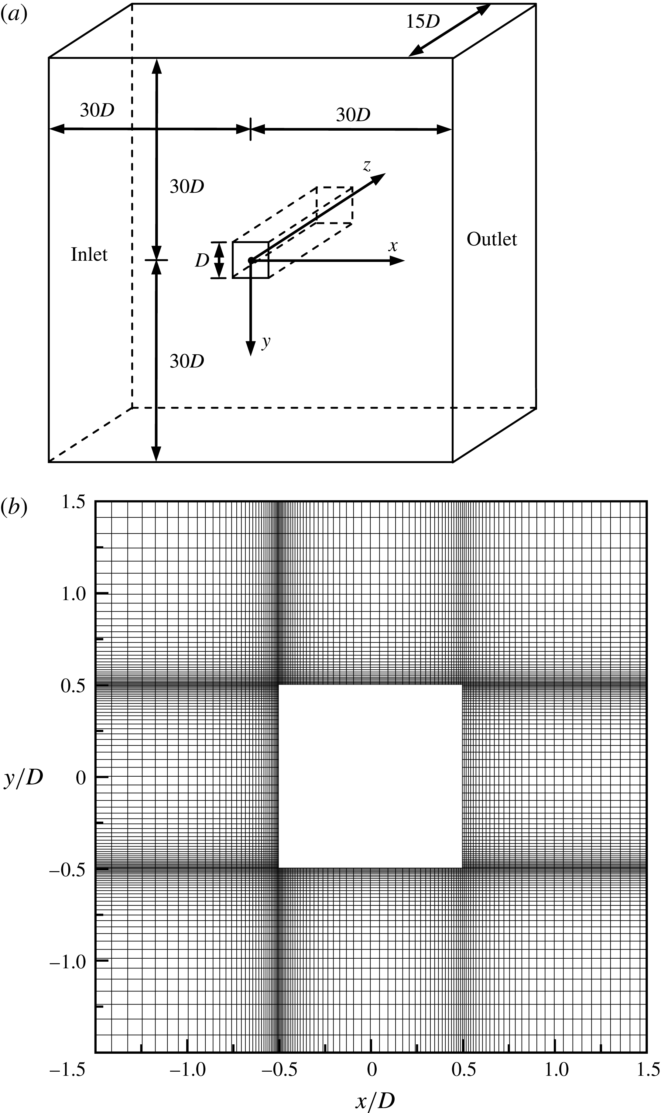
As shown in figure 1(a), a hexahedral computational domain of
 $(L_{x},L_{y},L_{z})=(60D,60D,15D)$
, with
 $L_{x}$
,
 $L_{y}$
and
 $L_{z}$
being the domain sizes in the
 $x$
-,
 $y$
- and
 $z$
-directions, respectively, is adopted for the simulations. The blockage ratio of the domain is
 $D/L_{y}\times 100\,\%=1.67\,\%$
, which is smaller than those of many studies listed in table 1. It will be further shown in § 2.4 that by reducing the blockage ratio from 1.67 % to 0.83 %, the
 $Re_{cr}$
values for Modes A and B would only vary 0.36 % and 0.35 %, respectively. For the spanwise domain length
 $L_{z}$
, Jiang et al. (Reference Jiang, Cheng, Draper, An and Tong2016) adopted an
 $L_{z}$
of
 $12D$
to accommodate three spanwise periods of the Mode A structures (with a spanwise wavelength of approximately
 $3.96D$
) for the case of a circular cylinder. Similarly, for the case of a square cylinder, an
 $L_{z}$
of
 $15D$
is adopted in the present study to accommodate three spanwise periods of Mode A. It will be shown in § 2.4 that the spanwise wavelength of Mode A for a square cylinder is approximately
 $4.96D$
(which is the wavelength at the left tip of the neutral instability curve for Mode A).
(a) Schematic model of the computational domain (not to scale), and (b) close-up view of the 2-D mesh near the cylinder.

The boundary conditions are specified as follows. At the inlet boundary, a uniform flow velocity
 $U$
is specified in the
 $x$
-direction. At the outlet, the Neumann boundary condition (i.e. zero normal gradient) is applied for the velocity, while the pressure is specified as a reference value of zero. Symmetry boundary conditions are applied at the top and bottom boundaries, while periodic boundary conditions are employed at the two lateral boundaries perpendicular to the cylinder span (Jiang, Cheng & An Reference Jiang, Cheng and An2017a
). A no-slip boundary condition is applied on the cylinder surface. The internal flow is stationary at the start of the simulation.
2.3 Mesh dependence study
A 2-D mesh is constructed first in the plane perpendicular to the cylinder axis (i.e. the
 $x$
–
 $y$
plane). For the 2-D mesh, the cylinder surface is discretized with 196 nodes. The height of the first layer of mesh next to the cylinder is
 $0.005D$
. The cell size at the two leading edges of the cylinder (where high velocity and pressure gradients take place) is
 $0.005D\times 0.005D$
. The cell expansion ratio in the whole domain is kept below 1.1. To capture detailed wake flow structures, a relatively high mesh resolution is used in the near wake by specifying a streamwise mesh size varying linearly from
 $0.05D$
at
 $x/D=1-0.1D$
at
 $x/D=7$
. A total of 43 922 cells are used for the 2-D mesh. A close-up view of the mesh near the cylinder is shown in figure 1(b).
It has been reported in previous studies that for 2-D simulations, the vortex shedding process changes from a regular periodic state into an irregular state as
 $Re$
exceeds a certain value, e.g. 225–250 in Robichaux et al. (Reference Robichaux, Balachandar and Vanka1999), 250–300 in Sohankar et al. (Reference Sohankar, Norberg and Davidson1999) and 210–218 in Saha, Muralidhar & Biswas (Reference Saha, Muralidhar and Biswas2000). Sohankar et al. (Reference Sohankar, Norberg and Davidson1999) attributed this phenomenon to the restriction of a 2-D domain. They also found that beyond this critical
 $Re$
the time-averaged flow field becomes asymmetric about the wake centreline. In the present study, this critical
 $Re$
is found at
 $Re=250{-}275$
. Therefore, a 2-D mesh dependence study at
 $Re=400$
(the highest
 $Re$
considered in this study) may be misleading, and a 3-D mesh dependence study will be conducted directly.
The 3-D mesh is constructed by replicating the 2-D mesh along the
 $z$
-axis, resulting in an identical mesh resolution in all planes perpendicular to the spanwise direction. The cell size in the spanwise direction (
 $\unicode[STIX]{x0394}z$
) is
 $0.125D$
. This results in a total of 120 mesh layers along the spanwise direction, which is the same as that used in Jiang et al. (Reference Jiang, Cheng, Draper, An and Tong2016) for a circular cylinder. A mesh dependence study regarding this reference mesh is carried out at
 $Re=400$
with the following two variations:
-
(i) A mesh refined in the
$z$
-direction, through reducing
$\unicode[STIX]{x0394}z$
from
$0.125D$
to
$0.0625D$
. -
(ii) A mesh refined in the
$x$
–
$y$
plane. This mesh has a number of cells in both
$x$
- and
$y$
-directions 1.5 times that of the reference mesh. Specifically, the number of cells around the cylinder surface is increased by 1.5 times, while the height of the first layer of mesh next to the cylinder is reduced by 1.5 times. For this case, the time step (
$\unicode[STIX]{x0394}t$
) is also reduced by 1.5 times so as to satisfy the same Courant–Friedrichs–Lewy (CFL) limit, which is to keep the CFL number less than 0.5 for all the cells in the computational domain. The CFL number is defined as: (2.3)where
$$\begin{eqnarray}CFL=\frac{|u|\unicode[STIX]{x0394}t}{\unicode[STIX]{x0394}l},\end{eqnarray}$$
$|u|$
is the magnitude of the velocity through a cell, and
$\unicode[STIX]{x0394}l$
is the cell size in the direction of the velocity.


Since the fully developed 3-D flow may be irregular, at least 800 non-dimensional time units (defined as
 $t^{\ast }=Ut/D$
) of the fully developed flow were used to calculate the statistical stationary hydrodynamic forces on the cylinder, including the drag and lift force coefficients (
 $C_{D}$
and
 $C_{L}$
) and the Strouhal number (
 $St$
), which are defined as:
 $$\begin{eqnarray}\displaystyle & \displaystyle C_{D}=\frac{F_{D}}{\frac{1}{2}\unicode[STIX]{x1D70C}DU^{2}L_{z}} & \displaystyle\end{eqnarray}$$
 $$\begin{eqnarray}\displaystyle & \displaystyle C_{L}=\frac{F_{L}}{\frac{1}{2}\unicode[STIX]{x1D70C}DU^{2}L_{z}} & \displaystyle\end{eqnarray}$$
 $$\begin{eqnarray}\displaystyle & \displaystyle St=\frac{f_{L}D}{U}, & \displaystyle\end{eqnarray}$$
where
 $F_{D}$
and
 $F_{L}$
are the integrated drag force and lift force on the entire cylinder, respectively, and
 $f_{L}$
is the frequency of the fluctuating lift force. These flow properties are defined based on the approaching flow velocity (
 $U$
) and the length scale of the cylinder perpendicular to the approaching flow (
 $D$
, namely the side length of the square cylinder). For irregular 3-D flows,
 $f_{L}$
is determined as the peak frequency derived from the fast Fourier transform (FFT) of the time history of
 $C_{L}$
. The time-averaged drag and lift coefficients are denoted as
 $\overline{C_{D}}$
and
 $\overline{C_{L}}$
, respectively. The root-mean-square lift coefficient
 $C_{L}^{\prime }$
is defined as:
 $$\begin{eqnarray}C_{L}^{\prime }=\sqrt{\frac{1}{N}\mathop{\sum }_{i=1}^{N}(C_{L,i}-\overline{C_{L}})^{2}},\end{eqnarray}$$
where
 $N$
is the number of values in the time history for the calculation of the root-mean-square quantity.
As shown in table 2, the hydrodynamic forces calculated with the two refined meshes are very close to those calculated with the reference mesh (relative differences are within 1 % for
 $St$
and
 $\overline{C_{D}}$
, and within 4 % for
 $C_{L}^{\prime }$
). In addition, the sufficiency of the statistical data range of at least 800 non-dimensional time units (called full length of data in table 2) is examined by calculating the hydrodynamic forces with only the second half of the time history (of at least 400 non-dimensional time units, called second half of data in table 2). The close agreement between the results calculated with the full length of data and the second half of data (relative differences are within 1 % for
 $St$
and
 $\overline{C_{D}}$
, and within 2 % for
 $C_{L}^{\prime }$
) suggests that the statistical data ranges are sufficient.
Results of the 3-D mesh dependence study at
 $Re=400$
.

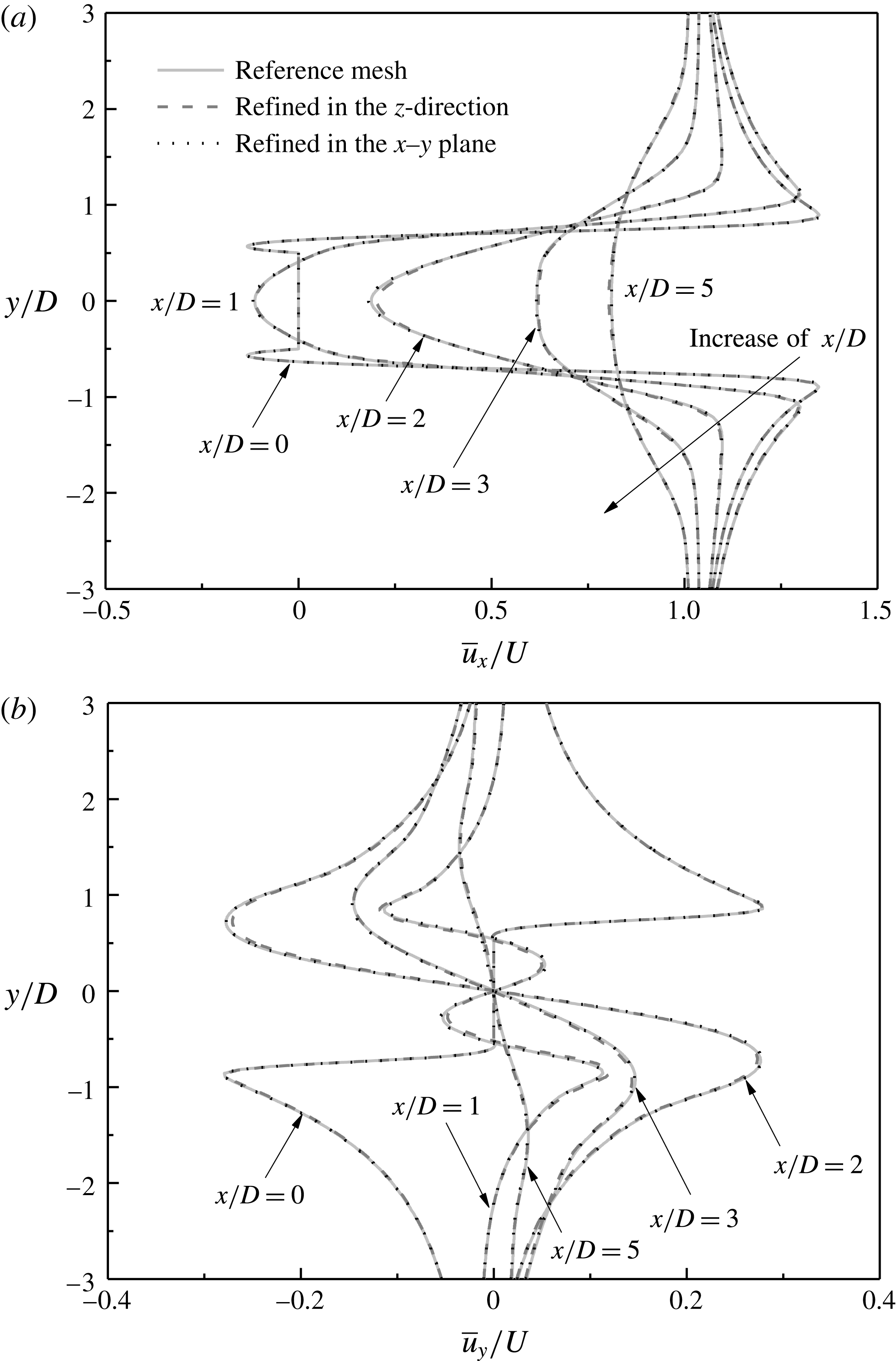
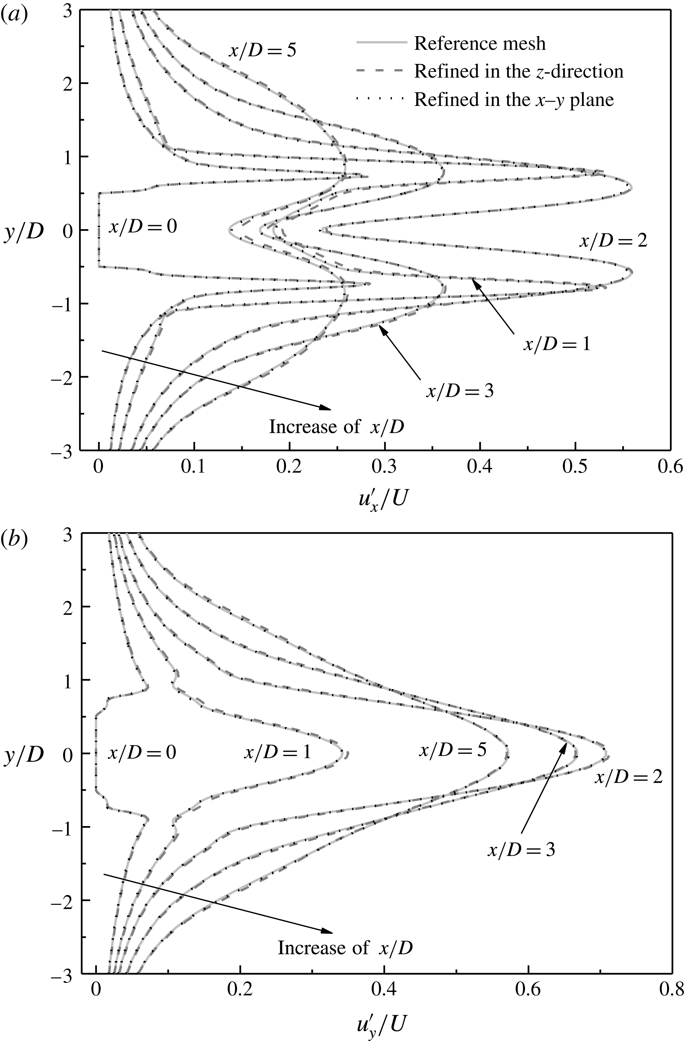
Furthermore, the mesh resolution in the cylinder wake is examined with velocity profiles sampled at streamwise locations
 $x/D=0$
, 1, 2, 3 and 5 for the three cases listed in table 2. The time-averaged and root-mean-square velocity profiles are plotted in figures 2 and 3, respectively. The time-averaged streamwise and transverse velocities are denoted as
 $\overline{u_{x}}$
and
 $\overline{u_{y}}$
, respectively, while the root-mean-square streamwise and transverse velocities are calculated as:
 $$\begin{eqnarray}\displaystyle & \displaystyle u_{x}^{\prime }=\sqrt{\frac{1}{N}\mathop{\sum }_{i=1}^{N}(u_{x,i}-\overline{u_{x}})^{2}}, & \displaystyle\end{eqnarray}$$
 $$\begin{eqnarray}\displaystyle & \displaystyle u_{y}^{\prime }=\sqrt{\frac{1}{N}\mathop{\sum }_{i=1}^{N}(u_{y,i}-\overline{u_{y}})^{2}}. & \displaystyle\end{eqnarray}$$
Note that each point of
 $\overline{u_{x}}$
,
 $\overline{u_{y}}$
,
 $u_{x}^{\prime }$
and
 $u_{y}^{\prime }$
on the velocity profiles is a value averaged over the spanwise direction.
As shown in figures 2 and 3, very good agreements of the near-wake velocity profiles are observed for the three cases listed in table 2. Hence the reference mesh is considered to be sufficient and is adopted in the present DNS study.
Time-averaged velocity profiles at streamwise locations
 $x/D=0,1,2,3$
and 5 for the three cases listed in table 2: (a) time-averaged streamwise velocity profiles, and (b) time-averaged transverse velocity profiles. Each point on the velocity profiles is a value averaged over the spanwise direction.

Root-mean-square velocity profiles at streamwise locations
 $x/D=0$
, 1, 2, 3 and 5 for the three cases listed in table 2: (a) root-mean-square streamwise velocity profiles, and (b) root-mean-square transverse velocity profiles. Each point on the velocity profiles is a value averaged over the spanwise direction.

2.4 Onset of wake instability
In the present study, the neutral instability curves for Modes A and B are re-examined by using DNS. For the prediction of the neutral instability curves, it is not necessary to use a long spanwise domain length (e.g.
 $L_{z}=15D$
) to simulate a few spanwise periods of the wake mode. For the purpose of minimizing the computational cost while retaining accuracy, the method proposed in Jiang et al. (Reference Jiang, Cheng, Draper and An2017b
) is adopted and is briefly introduced here. It is demonstrated in Jiang et al. (Reference Jiang, Cheng, Draper and An2017b
) that a neutral instability curve can be accurately predicted by resolving only a half of a spanwise period of the wake mode. Therefore, the meshes used for the prediction of the neutral instability curves are modified from the reference mesh introduced in § 2.3 (which uses
 $L_{z}=15D$
and 120 layers of mesh in the spanwise direction). The modified meshes adopt much shorter
 $L_{z}$
values together with symmetry boundary conditions for the two lateral boundaries perpendicular to the cylinder span (in replacement of the periodic boundary conditions), such that only a half of a spanwise period of the wake mode is allowed to develop in the domain. To resolve this, only 10 layers of mesh are used in the spanwise direction, which reduces the computational cost significantly. The sufficiency of 10 spanwise mesh layers will be demonstrated later on with a mesh dependence study.
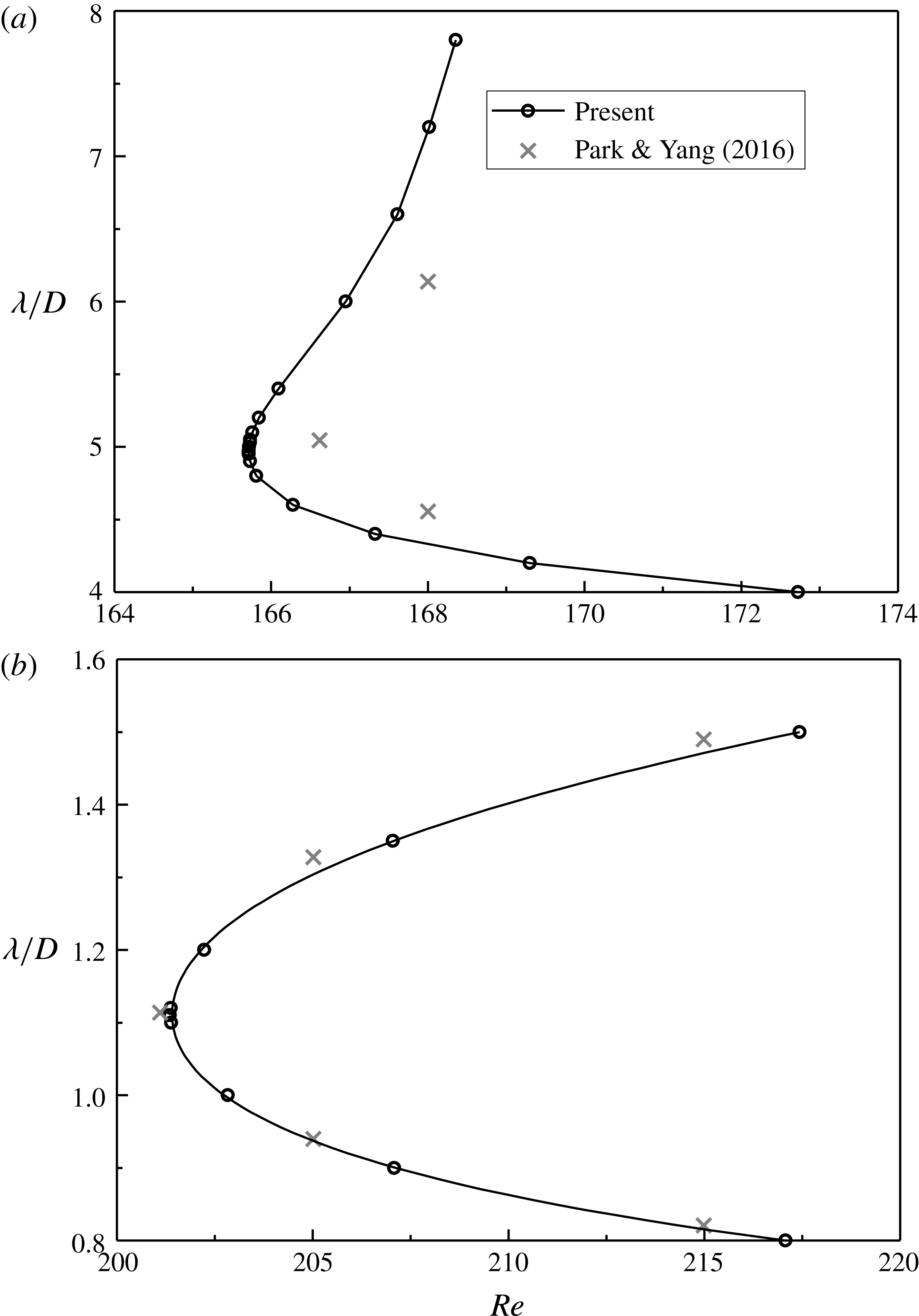
The neutral instability curves predicted by the present DNS are shown in figure 4. Each point on the neutral curve is obtained by specifying a fixed
 $L_{z}$
(i.e. a fixed spanwise wavelength of the wake mode
 $\unicode[STIX]{x1D706}=2L_{z}$
) and calculating a few cases with variations of
 $Re$
. For these cases, the exponential convergence/growth rates of the spanwise velocity amplitude sampled at a fixed point in the near wake of the cylinder are calculated. The
 $Re$
corresponding to the zero growth rate is the critical
 $Re$
at this fixed
 $\unicode[STIX]{x1D706}$
. More details and examples of the use of this method can be found in Jiang et al. (Reference Jiang, Cheng, Draper and An2017b
,Reference Jiang, Cheng, Draper and An
c
).
Neutral instability curves for (a) Mode A, and (b) Mode B. The neutral instability curves are shown for the ranges of
 $Re$
close to the left tip.

For an unconfined flow, the onset point of wake instability
 $Re_{cr}$
and the corresponding most unstable spanwise wavelength of the wake mode
 $(\unicode[STIX]{x1D706}/D)_{cr}$
can be found at the left tip of the neutral curve. As shown in figure 4, the
 $Re_{cr}$
and
 $(\unicode[STIX]{x1D706}/D)_{cr}$
values predicted by the present DNS are
 $(Re_{cr},(\unicode[STIX]{x1D706}/D)_{cr})=(165.7,4.96)$
for Mode A and
 $(Re_{cr},(\unicode[STIX]{x1D706}/D)_{cr})=(201.4,1.11)$
for Mode B.
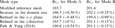
A mesh dependence study on the
 $Re_{cr}$
values for Modes A and B is carried out with the following three variations to the modified reference mesh:
-
(i) A mesh with an increase in the domain size, through doubling the distances from the cylinder centre to the inlet, outlet, top and bottom boundaries (each from
$30D$
to
$60D$
). -
(ii) A mesh refined in the
$x$
–
$y$
plane, through doubling the cell numbers in both the
$x$
- and
$y$
-directions. For this case, the time step is reduced by half so as to keep the CFL number less than 0.5. -
(iii) A mesh refined in the
$z$
-direction, through doubling the mesh layers in the spanwise direction (from 10 to 20).


Table 3 lists the
 $Re_{cr}$
values calculated with different meshes. The relative differences of
 $Re_{cr}$
with respect to those calculated with the modified reference mesh are all less than 1 %. In addition, the
 $Re_{cr}$
values predicted by Park & Yang (Reference Park and Yang2016) through stability analysis are also within 0.6 % of the present DNS results (table 3). Furthermore, the neutral instability curves predicted by the present DNS and by Park & Yang (Reference Park and Yang2016) display very similar trends (figure 4).
Mesh dependence of the
 $Re_{cr}$
values for Modes A and B. The relative difference of
 $Re_{cr}$
with respect to that calculated with the modified reference mesh is shown in the brackets.

3 Numerical results
3.1 Three-dimensional wake transition
The 3-D wake transition process and mode interactions are examined for
 $Re$
up to 400. For each individual case, the fully developed flow is obtained by simulating the case for at least 1000 non-dimensional time units. After that, at least another 1000 non-dimensional time units of the fully developed flow is used to analyse the characteristics of the flow. The flow is examined quantitatively via the statistically stationary flow properties and qualitatively through numerical flow visualization of the vorticity field. The streamwise vorticity
 $\unicode[STIX]{x1D714}_{x}$
, transverse vorticity
 $\unicode[STIX]{x1D714}_{y}$
and spanwise vorticity
 $\unicode[STIX]{x1D714}_{z}$
used in this paper are defined in a dimensionless form:
 $$\begin{eqnarray}\displaystyle & \displaystyle \unicode[STIX]{x1D714}_{x}=\left(\frac{\unicode[STIX]{x2202}u_{z}}{\unicode[STIX]{x2202}y}-\frac{\unicode[STIX]{x2202}u_{y}}{\unicode[STIX]{x2202}z}\right)\frac{D}{U}, & \displaystyle\end{eqnarray}$$
 $$\begin{eqnarray}\displaystyle & \displaystyle \unicode[STIX]{x1D714}_{y}=\left(\frac{\unicode[STIX]{x2202}u_{x}}{\unicode[STIX]{x2202}z}-\frac{\unicode[STIX]{x2202}u_{z}}{\unicode[STIX]{x2202}x}\right)\frac{D}{U}, & \displaystyle\end{eqnarray}$$
 $$\begin{eqnarray}\displaystyle & \displaystyle \unicode[STIX]{x1D714}_{z}=\left(\frac{\unicode[STIX]{x2202}u_{y}}{\unicode[STIX]{x2202}x}-\frac{\unicode[STIX]{x2202}u_{x}}{\unicode[STIX]{x2202}y}\right)\frac{D}{U}. & \displaystyle\end{eqnarray}$$
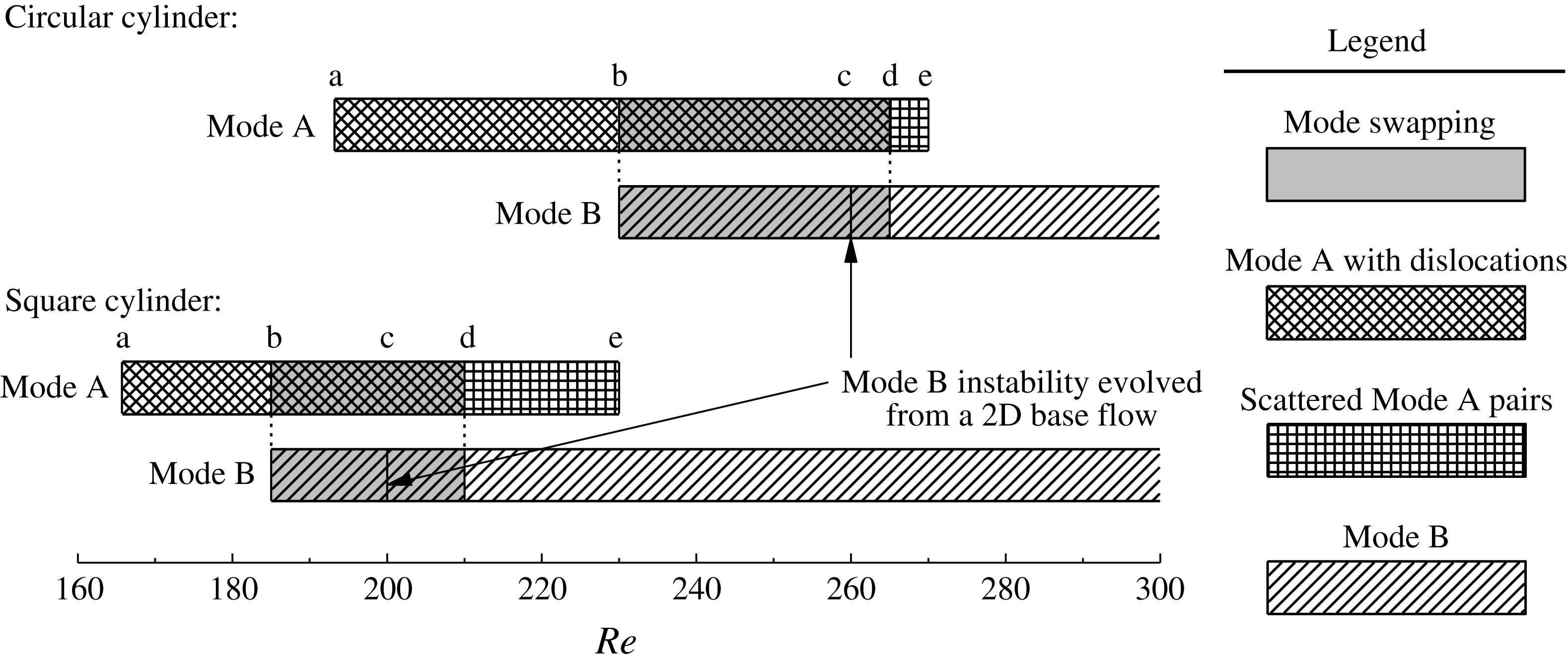
Figure 5 summarizes the 3-D wake transition regimes for a circular and a square cylinder. The transition regimes for a circular cylinder are plotted based on the DNS results reported in Jiang et al. (Reference Jiang, Cheng, Draper, An and Tong2016). For both cases, the wake flow undergoes a transition sequence of ‘Mode A*
 $\rightarrow$
mode swapping
 $\rightarrow$
Mode B’ with increasing
 $Re$
. The first 3-D instability mode, namely Mode A (before the evolution to Mode A* with time), originates from a 2-D flow and is due to an elliptic instability of the primary vortex cores and the formation of streamwise vortex pairs through Biot–Savart induction (Williamson Reference Williamson1996; Leweke & Williamson Reference Leweke and Williamson1998; Thompson, Leweke & Williamson Reference Thompson, Leweke and Williamson2001a
). The wake transition process for the square cylinder case is studied with the aid of figure 5, and several features of the wake transition process are summarized below:
Three-dimensional wake transition regimes for a circular and a square cylinder. The results for a circular cylinder are based on the DNS results reported in Jiang et al. (Reference Jiang, Cheng, Draper, An and Tong2016).

-
(i) For a fully resolved 3-D flow, a gradual wake transition from Mode A* to Mode B takes place at
$Re=185{-}210$
. In contrast, when the Mode B instability evolves from a 2-D base flow directly, the onset of Mode B occurs at
$Re\sim 200$
, for example the Mode B instability predicted in § 2.4 or through Floquet stability analysis (see table 1). For a fully resolved 3-D flow, the early development of Mode B for
$Re$
in the range of approximately 185–200 is expected, since Mode B, which is due to a hyperbolic instability of the braid shear layer region (Williamson Reference Williamson1996; Leweke & Williamson Reference Leweke and Williamson1998; Thompson et al.
Reference Thompson, Leweke and Williamson2001a
), is destabilized at
$Re<200$
by the streamwise vortices of Mode A that develop in the braid shear layer region (Jiang et al.
Reference Jiang, Cheng, Draper, An and Tong2016). As shown in figure 5, this feature is also observed for the case of a circular cylinder. Obviously the onset point of Mode B for a square cylinder of
$Re\geqslant 200$
predicted by previous DNS and experimental studies (table 1) is not in line with the mechanism for the early development of Mode B. -
(ii) The range of
$Re$
for the early development of Mode B (i.e. the range of points b–c in figure 5) for a square cylinder (of
$\unicode[STIX]{x0394}Re\sim 15$
) is smaller than that for a circular cylinder (of
$\unicode[STIX]{x0394}Re\sim 30$
). Nevertheless, for both cases point ‘b’ in figure 5 is located at approximately the middle of the range of points a–c. This is possibly due to the competition of the two modes, i.e. Mode B can be competitive down to the mid-point of the range of points a–c, but Mode A* dominants the lower half of this range. -
(iii) For both cases, the mode swapping regime ends at a point (point ‘d’ in figure 5) slightly above the point where Mode B becomes globally unstable (point ‘c’ in figure 5).
-
(iv) Beyond the mode swapping regime, Mode B is the dominant mode, while Mode A may be observed in the form of scattered vortex pairs for a small range of
$Re$
(i.e. the range of points d–e in figure 5). Compared with the circular cylinder case, the range of points d–e for a square cylinder is longer, possibly because it is closer to the onset of Mode A so that Mode A is more competitive. It is also noted that Mode QP is not observed for the entire range of
$Re$
(up to 400) considered in this study.


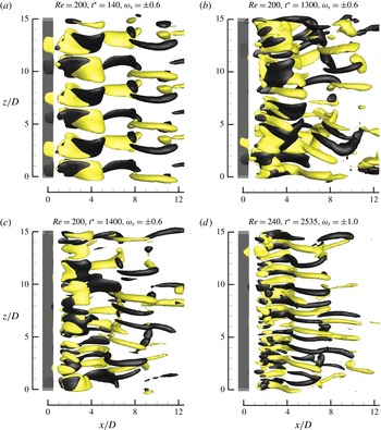
Iso-surfaces of
 $\unicode[STIX]{x1D714}_{x}$
for (a) ordered Mode A (before the evolution to Mode A* with time) at
 $Re=200$
, (b) Mode A* (with dislocation) at
 $Re=200$
, (c) a mixture of Modes A and B (without dislocation) at
 $Re=200$
and (d) disordered Mode B at
 $Re=240$
. Dark grey and light yellow denote positive and negative values, respectively. The flow is from the left to the right past the cylinder on the left.

Figure 6 shows some typical wake structures captured by the iso-surfaces of
 $\unicode[STIX]{x1D714}_{x}$
. For
 $Re=200$
which involves mode swapping, the 3-D wake flow is initialized with the ordered Mode A structure (figure 6
a), followed by the swapping between the Mode A* flow (with dislocation) shown in figure 6(b) and a mixture of Modes A and B (without dislocation) shown in figure 6(c). Beyond the mode swapping regime, increasingly disordered Mode B is observed (figure 6
d).
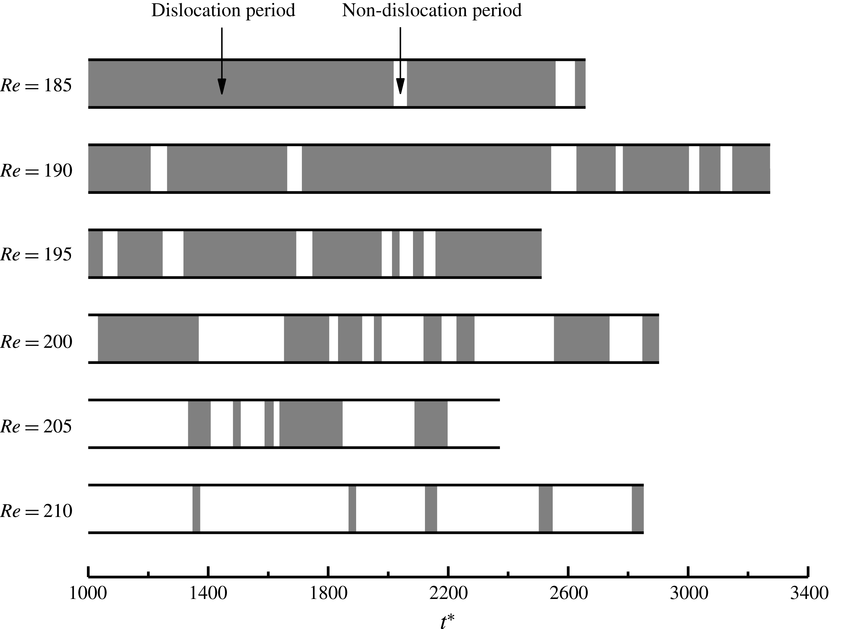
Time evolution of the vortex dislocations for the cases in the mode swapping regime.

The mode swapping regime is further examined by identifying the time evolution of the vortex dislocations for each case. This is shown in figure 7, with shaded and clear periods representing the dislocation periods (e.g. figure 6
b) and non-dislocation periods (e.g. figure 6
c), respectively. For
 $Re=185{-}195$
, the dislocation periods emerge cyclically, which is similar to the circular cylinder case reported in Jiang et al. (Reference Jiang, Cheng, Draper, An and Tong2016). Based on a relatively weak and ordered Mode A flow, each dislocation period begins with the development of a local vortex dislocation originating from a specific Mode A vortex loop after it grows in strength for a short period of time. After the dislocation period, vortex dislocation is replaced by a mixture of Modes A and B, where Mode B is destabilized by the streamwise vortices of Mode A (Jiang et al.
Reference Jiang, Cheng, Draper, An and Tong2016). However, the Mode B structure in the mixture may decay with time, as the source for the early destabilization of Mode B disappears. The next cycle begins when all the Mode B structures die out and the Mode A structures start to grow at the locations where Mode B disappears.
For
 $Re=200{-}210$
, however, the dislocation periods may or may not emerge based on such cycles. As Mode B becomes globally unstable at
 $Re\sim 200$
, the Mode B structures in the mixture of Modes A and B (e.g. figure 6
c) may not have to decay with time and result in a new cycle. This factor contributes to the decrease in the probability of occurrence of vortex dislocations.
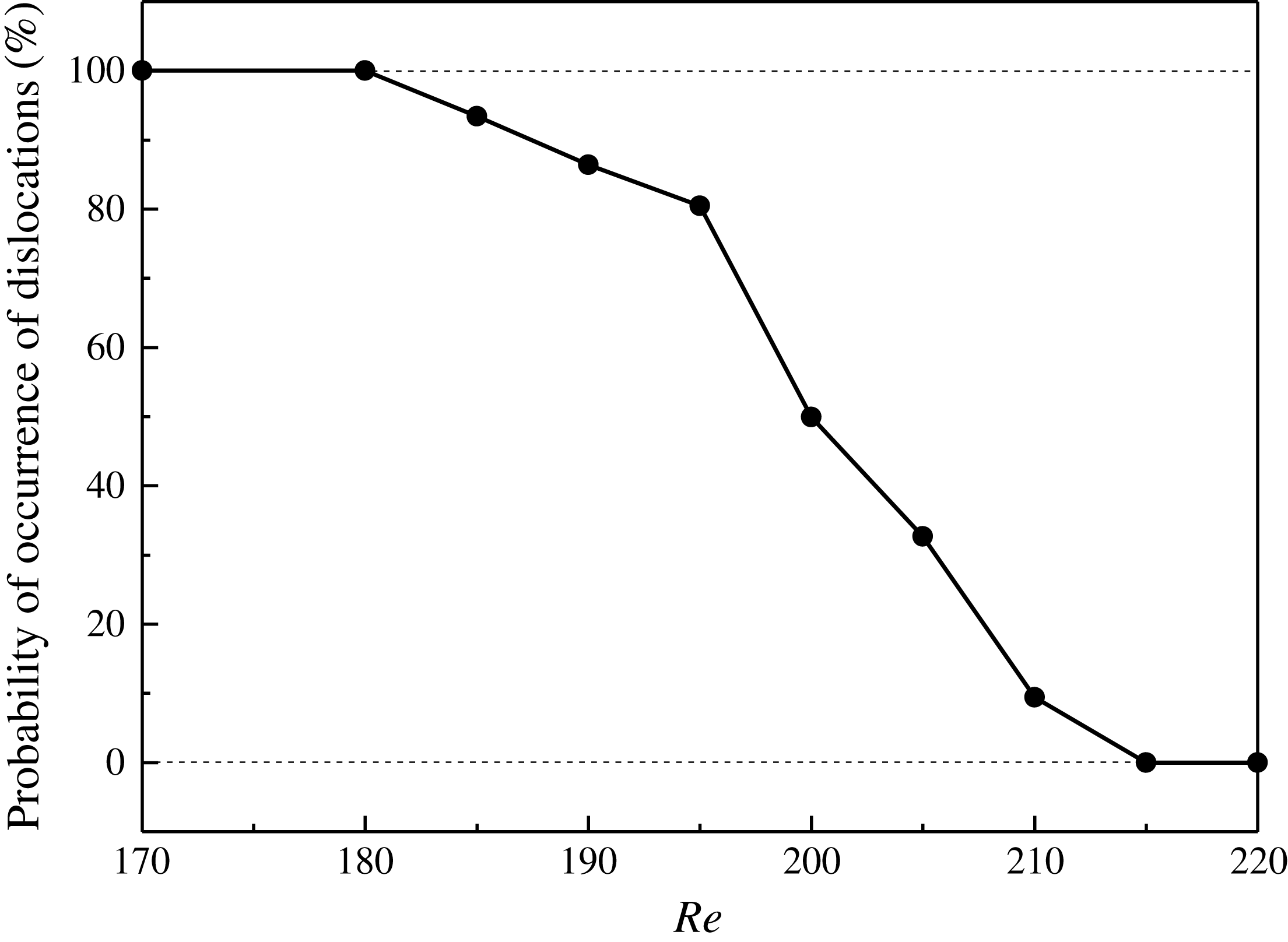
Probability of occurrence of vortex dislocations as a function of
 $Re$
.

As can be seen more clearly in figure 8, the probability of occurrence of vortex dislocations decreases monotonically with increasing
 $Re$
. For
 $Re=185{-}195$
, the wake structure is dominated by vortex dislocations, with a probability of occurrence of more than 80 %. Beyond that, a sharp decrease in the probability of occurrence of vortex dislocations is observed.
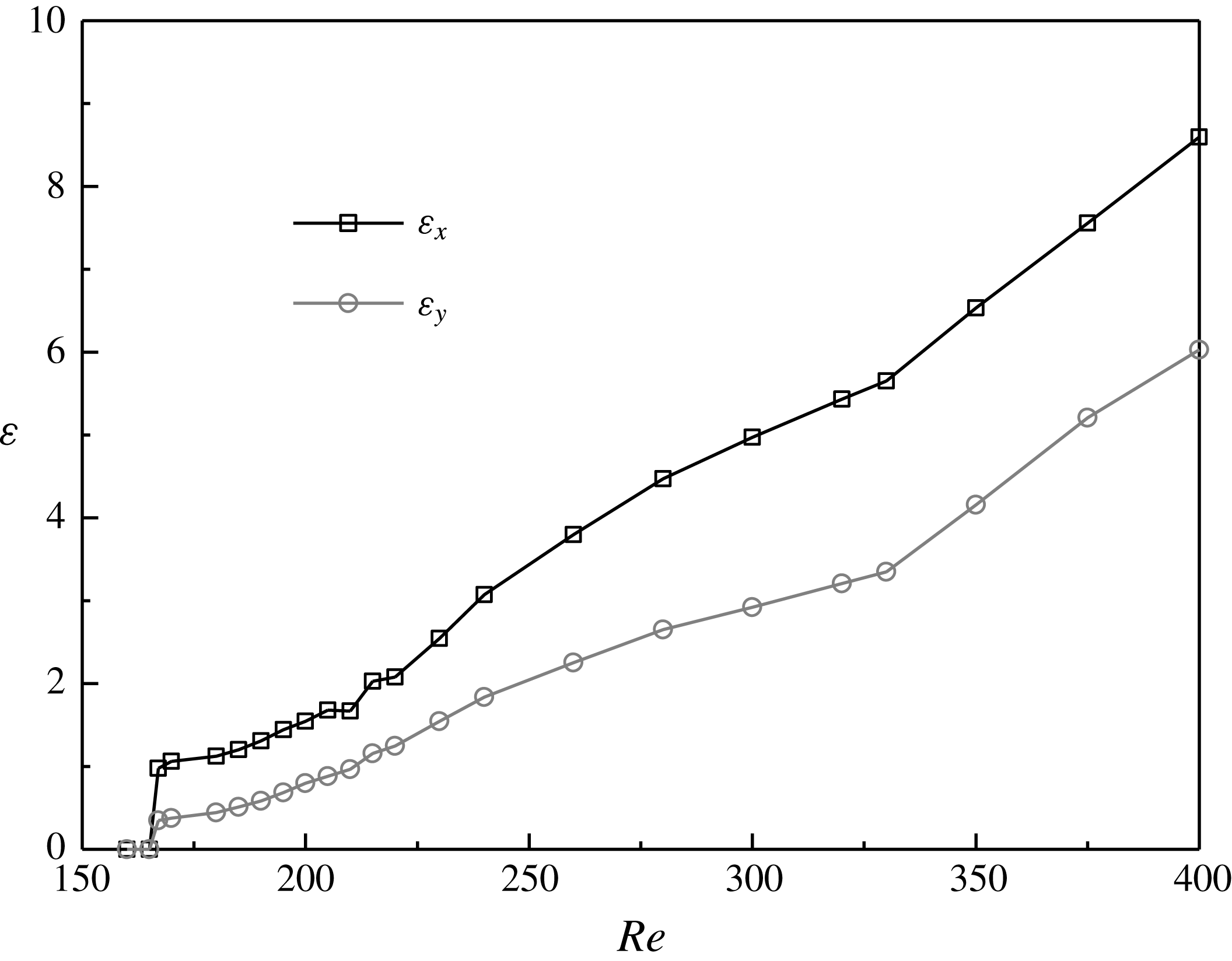
Variations of the time-averaged streamwise and transverse enstrophies with
 $Re$
.

3.2 Three-dimensionality of the flow
The variation of the flow three-dimensionality with
 $Re$
is examined in figure 9, where the three-dimensionality is represented by the time-averaged near-wake streamwise and transverse enstrophies (
 $\unicode[STIX]{x1D700}_{x}$
and
 $\unicode[STIX]{x1D700}_{y}$
) per unit span length. The enstrophies are defined as:
 $$\begin{eqnarray}\displaystyle & \displaystyle \unicode[STIX]{x1D700}_{x}=\frac{1}{2L_{z}}\int _{V}\unicode[STIX]{x1D714}_{x}^{2}\,\text{d}V & \displaystyle\end{eqnarray}$$
 $$\begin{eqnarray}\displaystyle & \displaystyle \unicode[STIX]{x1D700}_{y}=\frac{1}{2L_{z}}\int _{V}\unicode[STIX]{x1D714}_{y}^{2}\,\text{d}V, & \displaystyle\end{eqnarray}$$
where
 $V$
is the volume of the flow field of interest, which is the near-wake region of
 $x/D=0{-}5$
and the entire lengths in the
 $y$
- and
 $z$
-directions for the present study. As shown in figure 9, the flow three-dimensionality increases gradually with increasing
 $Re$
.
In contrast, a critical condition is observed for the case of a circular cylinder at
 $Re=265{-}270$
(Williamson Reference Williamson1996; Jiang et al.
Reference Jiang, Cheng, Draper, An and Tong2016), where a transition from the disappearance of Mode A* to the emergence of increasingly disordered Mode B results in a very weak flow three-dimensionality at this particular small range of
 $Re$
(Jiang et al.
Reference Jiang, Cheng, Draper, An and Tong2016). However, as reflected in figure 9, such a critical condition is not observed for the square cylinder case. Such a difference can be explained with the aid of figure 5. For the circular cylinder case, Mode A (and Mode A*), which has a relatively strong flow three-dimensionality, is no longer dominant at the point where Mode B becomes globally unstable, while at this point Mode B is still largely ordered and therefore exhibits a very weak flow three-dimensionality. For the square cylinder case, however, Mode A (and Mode A*) is still dominant at the point where Mode B becomes globally unstable. Beyond the mode swapping regime, which is approximately
 $\unicode[STIX]{x0394}Re\geqslant 10$
above the onset of the global instability of Mode B, the Mode B structures become increasingly disordered, while scattered Mode A structures still remain in the flow. Both factors contribute to a sustained high level of flow three-dimensionality at this point. With a further increase in
 $Re$
, the increasingly disordered Mode B becomes the sole reason for the continuous increase in the flow three-dimensionality shown in figure 9.
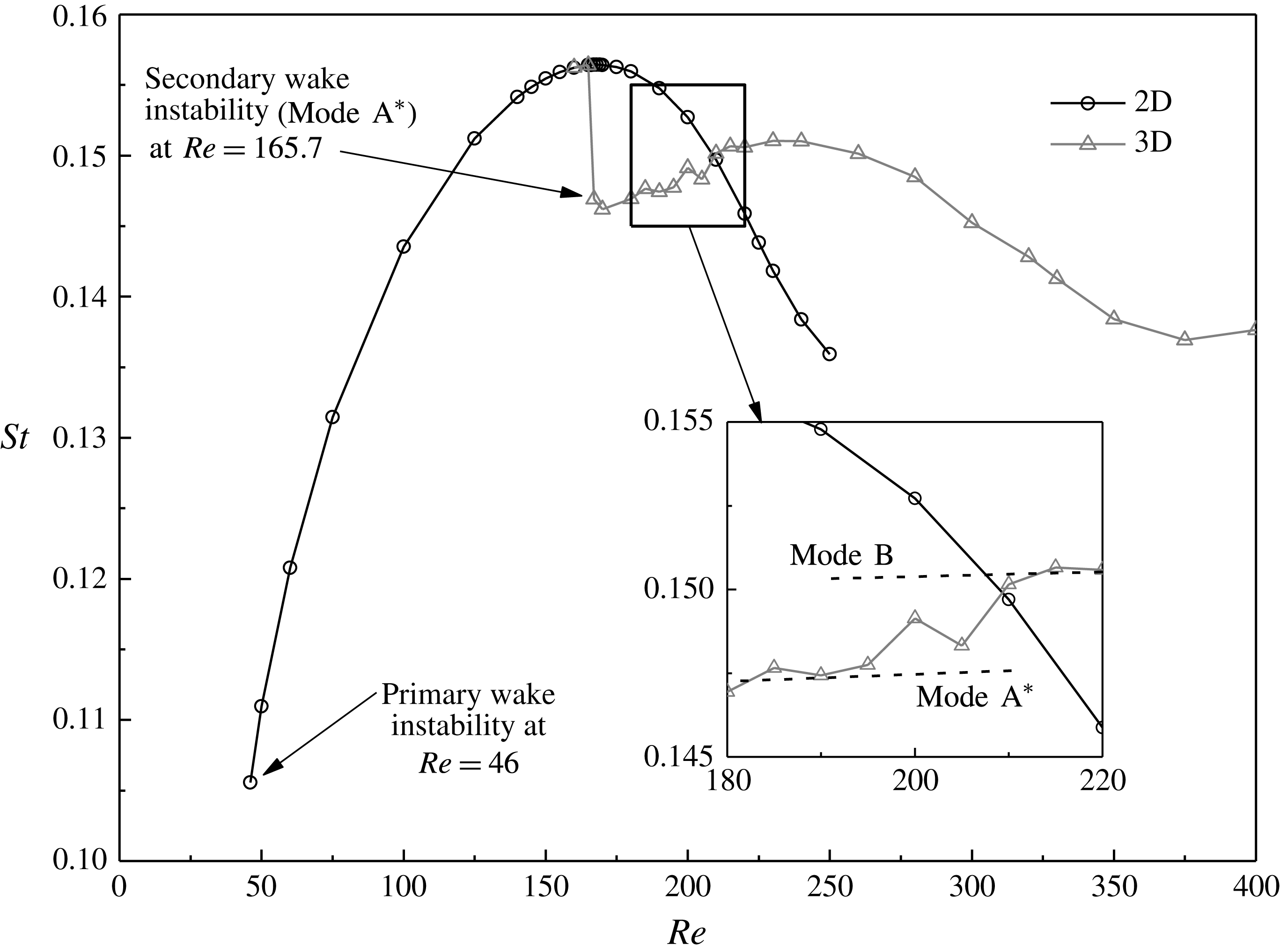
Two- and three-dimensional
 $St{-}Re$
relationships over the laminar and 3-D wake transition regimes.

3.3 The
$St{-}Re$
relationship

Figure 10 shows the 2-D and 3-D
 $St{-}Re$
relationships over the laminar and 3-D wake transition regimes for flow past a square cylinder. The 2-D simulations are performed for
 $Re\leqslant 250$
above which the vortex shedding process becomes irregular due to the restriction of a 2-D domain (Sohankar et al.
Reference Sohankar, Norberg and Davidson1999). In the present study, the 3-D
 $St{-}Re$
relationship shown in figure 10 is analysed in terms of the gradual/sudden variations of the curve at the onset of the Mode A* wake instability and over the wake transition process from Mode A* to Mode B.
At the onset of Mode A* of
 $Re_{cr}=165.7$
, a sudden drop of the 3-D
 $St$
value from its 2-D counterpart is observed in figure 10. This is consistent with the sudden increase in the flow three-dimensionality at this point (figure 9). As will be shown in § 3.4, the sudden increase in the flow three-dimensionality at this point is due to the subcritical nature of the Mode A* instability. The sudden increase in the flow three-dimensionality leads to a sudden decrease in the separating velocity and a sudden increase in the wake width for the 3-D flow, which results in a sudden decrease in the 3-D
 $St$
value. Similar features are also observed in Jiang & Cheng (Reference Jiang and Cheng2017) for flow past a circular cylinder.
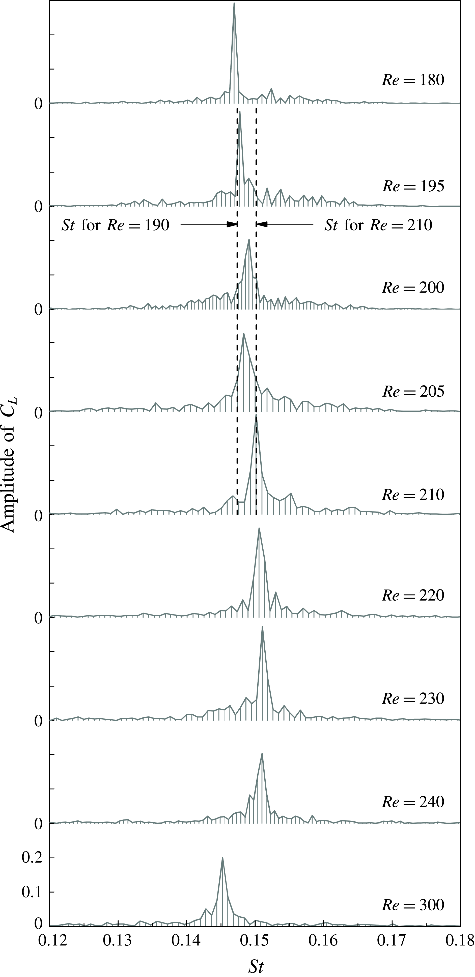
Frequency spectra of
 $C_{L}$
for
 $Re$
in the range of 180–300.

However, a difference with the circular cylinder case is that for the square cylinder case the 3-D
 $St{-}Re$
curve is continuous over the mode swapping regime (figure 10). Figure 11 shows some of the frequency spectra of
 $C_{L}$
which are used to determine the 3-D
 $St$
values. Each vertical line under the frequency spectrum represents a discrete point on the spectrum curve, since the FFT analysis is performed based on a finite data range (1200 to 1900 non-dimensional time units) of the time history of
 $C_{L}$
. Over the wake transition regimes, including the gradual wake transition process from Mode A* to Mode B at
 $Re=185{-}210$
, only a single frequency peak is observed for each case, and correspondingly a single 3-D
 $St{-}Re$
curve is observed in figure 10. This appears to be a major difference compared with the case of a circular cylinder for which two frequency peaks (a lower peak for Mode A* and a higher peak for Mode B) and correspondingly a discontinuity in the 3-D
 $St{-}Re$
curve are observed in the mode swapping regime (Williamson Reference Williamson1996).
For the case of a square cylinder, relatively uniform
 $St$
values are observed for the following two ranges (see the inset of figure 10):
-
(i)
$Re=180{-}190$
, with the probability of occurrence of Mode A* of larger than 80 % (figure 8), i.e. generally before mode swapping. -
(ii)
$Re=210{-}220$
, with the probability of occurrence of Mode A* of smaller than 10 % (figure 8), i.e. generally after mode swapping.


Theoretically, two discontinuous segments of the
 $St{-}Re$
curve, which correspond to Mode A* and Mode B, respectively, may be extended from the two above-mentioned ranges (illustrated by the two dashed lines in the inset of figure 10), as is the case for a circular cylinder. However, for a square cylinder the difference in
 $St$
between the two segments of the
 $St{-}Re$
curve is extremely small. For example, the difference in
 $St$
between
 $Re=190$
and 210 is 0.0028. As shown in figure 11, the frequency spectra for both Mode
 $A^{\ast }(Re=180)$
and Mode B (
 $Re\geqslant 210$
) are broadband, having a distinct peak covering a small range of
 $St$
, along with small-scale fluctuations extending towards the two sides of the peak. Within the narrow range of
 $\unicode[STIX]{x0394}St=0.0028$
between the two modes (shown by the two vertical dashed lines in figure 11), the two broadband frequency peaks for the cases within the mode swapping regime would merge into a single broadband peak, and consequently a single and continuous 3-D
 $St{-}Re$
curve is observed in figure 10. In contrast, the difference in
 $St$
between the two modes for a circular cylinder is approximately 0.01 (see Williamson (Reference Williamson1996) and Jiang et al. (Reference Jiang, Cheng, Draper, An and Tong2016)), which would result in two distinguishable frequency peaks in the spectrum.
The continuous 3-D
 $St{-}Re$
curve for a square cylinder suggests that the method for the determination of the critical
 $Re$
for the onset of Mode B by examining the discontinuities of the
 $St{-}Re$
curve (e.g. Luo et al.
Reference Luo, Tong and Khoo2007) may be inappropriate when the vortex shedding frequencies of the two wake modes are very close. This may explain why the experimental study by Luo et al. (Reference Luo, Tong and Khoo2007) over-predicted the onset point for Mode B by
 $\unicode[STIX]{x0394}Re\sim 20$
.
3.4 Hysteresis effect
Since the experimental studies by Luo et al. (Reference Luo, Chew and Ng2003) and Luo et al. (Reference Luo, Tong and Khoo2007) drew opposite conclusions on the existence of hysteresis at the onset of the Mode A instability, the existence of hysteresis is re-examined in the present study with DNS.
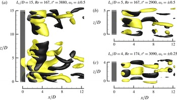
Iso-surfaces of
 $\unicode[STIX]{x1D714}_{x}$
for the fully developed 3-D flow structures at
 $Re$
slightly above
 $Re_{cr}$
. (a) Mode A*, with
 $L_{z}/D=15$
, (b) one spanwise period of ordered Mode A, with
 $L_{z}/D=5$
and (c) one spanwise period of ordered Mode A, with
 $L_{z}/D=4$
. Dark grey and light yellow denote positive and negative values, respectively. The flow is from the left to the right past the cylinder on the left. In (b) and (c), one half of the spanwise period of Mode A is distributed across the boundaries perpendicular to the cylinder span, since periodic boundary conditions are used.

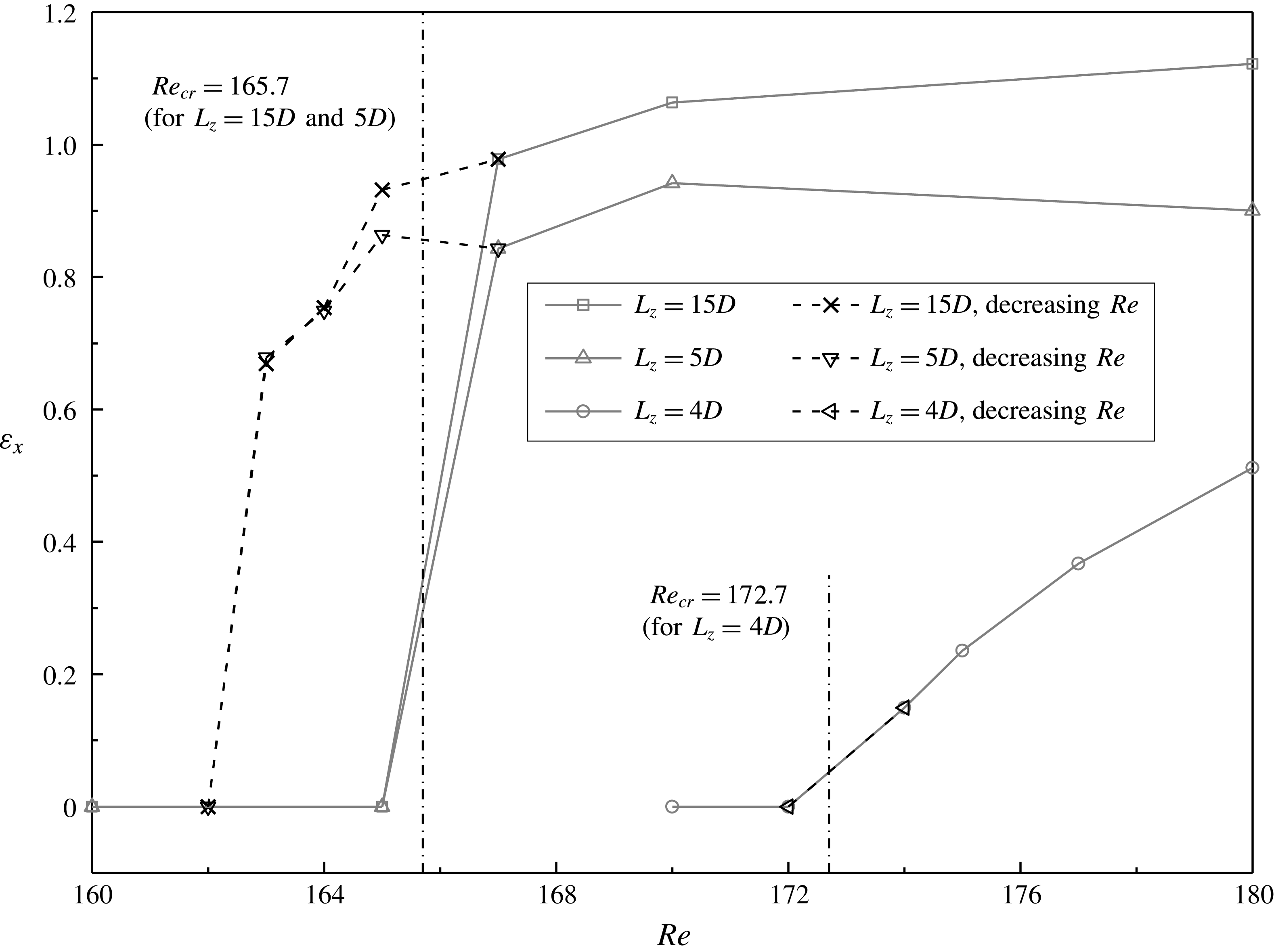
Variations of the time-averaged streamwise enstrophy with
 $Re$
for
 $Re$
close to the onset of Mode A.

The hysteresis at the onset of Mode A (of
 $Re_{cr}=165.7$
) is checked by adopting the fully developed Mode A* flow at
 $Re=167$
(figure 12
a) as the initial condition and reducing
 $Re$
by a small interval each time until the 3-D flow structure (i.e. the Mode A* structure) disappears naturally. For each case with a reduction in
 $Re$
, the simulation is run for at least 900 non-dimensional time units, and the three-dimensionality of the fully developed flow is quantified by the time-averaged streamwise enstrophy per unit span length (equation (3.4)). As shown in figure 13, a hysteresis loop of
 $\unicode[STIX]{x0394}Re\sim 3$
, namely between
 $Re=162{-}163$
and
 $Re_{cr}$
, is observed (with
 $L_{z}=15D$
).
The existence of hysteresis is also checked by adopting a series of cases with
 $L_{z}=5D$
(approximately the most unstable spanwise wavelength of Mode A), through which vortex dislocation is suppressed and the fully developed 3-D flow structure is represented by one spanwise period of ordered Mode A structures (figure 12
b). For this set of cases, a similar hysteresis loop is observed in figure 13, which suggests that hysteresis is irrelevant to the occurrence of vortex dislocation.
However, with a spanwise confinement of the Mode A structure by using
 $L_{z}=4D$
(approximately 80 % of the most unstable wavelength of Mode A), although the fully developed 3-D flow structure is also represented by one spanwise period of ordered Mode A structures (figure 12
c), hysteresis is not observed (figure 13). This is similar to the case of a circular cylinder, for which the hysteresis loop becomes smaller with decrease of the spanwise wavelength of Mode A and disappears at a spanwise wavelength of approximately 88 % of the most unstable wavelength of Mode A (Akbar, Bouchet & Dušek Reference Akbar, Bouchet and Dušek2011). These results suggest that hysteresis is also irrelevant to the wake flow mode. The supercritical behaviour for
 $L_{z}=4D$
(figure 13) is believed to be due to the confinement on the Mode A flow structure, such that the three-dimensionality of the Mode A flow is restricted, and a gradual rather than a sudden increase in the flow three-dimensionality is observed as
 $Re$
exceeds
 $Re_{cr}$
. It is worth mentioning that a supercritical Mode A instability is also observed for flow past a circular cylinder placed near to a moving wall with a gap-to-diameter ratio of 0.4 (Jiang et al.
Reference Jiang, Cheng, Draper and An2017d
), for which the Mode A flow structure is confined by the plane wall and the three-dimensionality of the Mode A flow increases gradually as
 $Re$
exceeds
 $Re_{cr}$
.
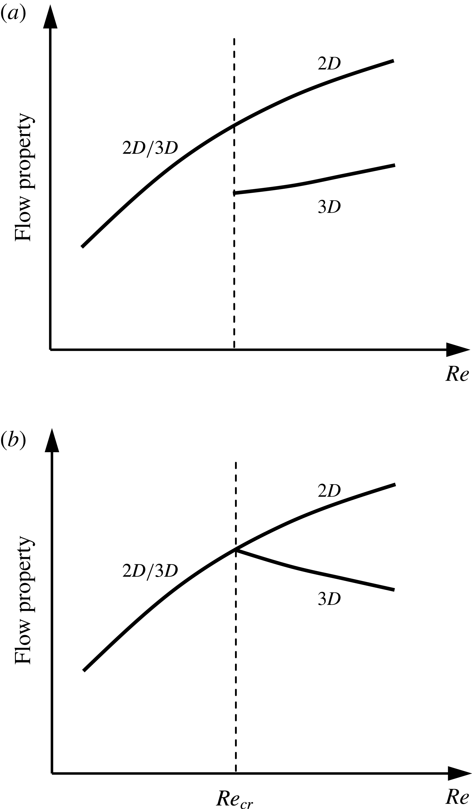
Sketch of the relationship between the flow property and
 $Re$
for (a) hysteretic flows, and (b) non-hysteretic flows.

As illustrated in figure 13, the sudden and gradual variations in the flow three-dimensionality correspond to subcritical (hysteretic) and supercritical (non-hysteretic) flows, respectively. Similar variation trends are also observed for other flow properties, such as the Strouhal number and hydrodynamic forces on the cylinder, since the flow properties are influenced by the flow three-dimensionality. When the flow is hysteretic, the relationship between the 3-D flow property and
 $Re$
displays a discontinuity at the onset of the wake instability (illustrated in figure 14
a; for example the 3-D
 $St{-}Re$
relationship with
 $L_{z}=15D$
as shown in figure 10). When the flow is non-hysteretic, the 3-D flow property deviates from its 2-D counterpart gradually at the onset of the wake instability (illustrated in figure 14
b; for example the Mode A instability for flow past a circular cylinder placed near to a moving wall with a gap-to-diameter ratio of 0.4 (Jiang et al.
Reference Jiang, Cheng, Draper and An2017d
)). In other words, the existence of hysteresis can be identified alternatively by examining the sudden/gradual variation of the 3-D flow properties at the onset of the wake instability, without having to carry out additional simulations for the reducing
 $Re$
branch.
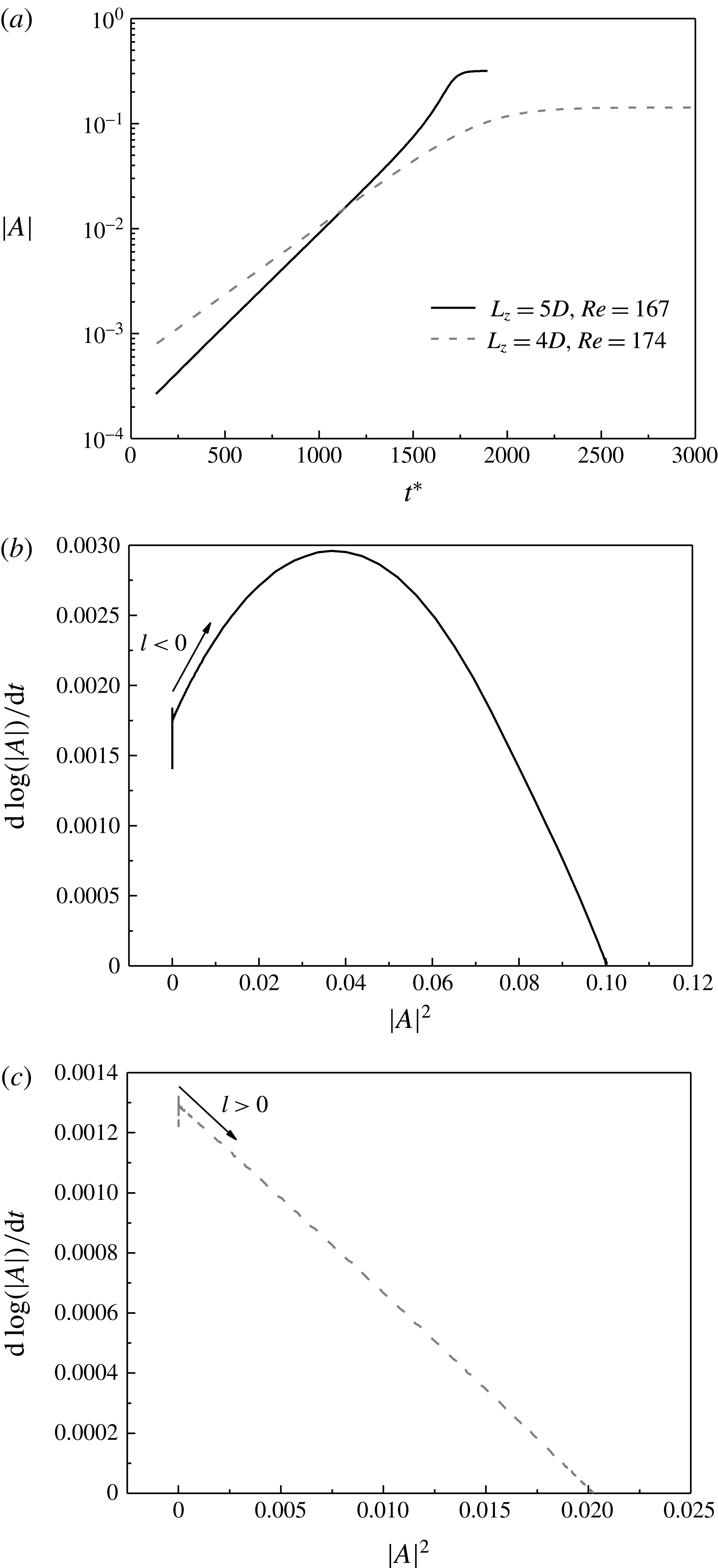
In the literature, the Landau model (Landau & Lifshitz Reference Landau and Lifshitz1976) has also been used to examine the hysteresis effect of wake instability modes for flow past bluff bodies (e.g. Dušek, Le Gal & Fraunié Reference Dušek, Le Gal and Fraunié1994; Henderson & Barkley Reference Henderson and Barkley1996; Thompson, Leweke & Provansal Reference Thompson, Leweke and Provansal2001b
; Sheard, Thompson & Hourigan Reference Sheard, Thompson and Hourigan2004; Carmo et al.
Reference Carmo, Sherwin, Bearman and Willden2008; Sheard et al.
Reference Sheard, Fitzgerald and Ryan2009). The Landau equation, which considers the amplitude
 $A(t)$
of a perturbation mode, is written up to third order as:
 $$\begin{eqnarray}\frac{\text{d}A}{\text{d}t}=(\unicode[STIX]{x1D70E}+\text{i}\unicode[STIX]{x1D714})A-l(1+\text{i}c)|A|^{2}A+\cdots \,,\end{eqnarray}$$
where
 $\unicode[STIX]{x1D70E}$
is the linear growth rate of the perturbation,
 $\unicode[STIX]{x1D714}$
is the angular oscillation frequency during the linear growth phase and
 $c$
is the Landau constant. The hysteresis of the wake instability mode can be determined based on the sign of the
 $l$
-coefficient. A positive
 $l$
indicates a supercritical (non-hysteretic) flow, while a negative
 $l$
indicates a subcritical (hysteretic) flow. The
 $l$
-coefficient is determined by plotting
 $(\text{d}\log |A|/\text{d}t)$
against
 $|A|^{2}$
, where the slope of the curve near to the
 $y$
-axis gives –
 $l$
. More details on the Landau equation can be found in Dušek et al. (Reference Dušek, Le Gal and Fraunié1994), Sheard et al. (Reference Sheard, Thompson and Hourigan2004) and Carmo et al. (Reference Carmo, Sherwin, Bearman and Willden2008).
By using the Landau equation, Sheard et al. (Reference Sheard, Fitzgerald and Ryan2009) reported a supercritical (non-hysteretic) bifurcation with a positive
 $l$
-coefficient for the Mode A instability for flow past a square cylinder, which appears at odds with the present results for an unconfined Mode A instability (with
 $L_{z}=15D$
and
 $5D$
). A possible speculation is that the spanwise wavelength for Mode A used in Sheard et al. (Reference Sheard, Fitzgerald and Ryan2009) may be smaller than the most unstable wavelength of Mode A, such that a confined Mode A was developed.
Results for the unconfined Mode A flow with
 $L_{z}=5D$
and
 $Re=167$
, and the confined Mode A flow with
 $L_{z}=4D$
and
 $Re=174$
. (a) The growth and saturation of the mode amplitude. (b) The derivative of the amplitude logarithm against the square of the amplitude for the unconfined flow, which indicates a subcritical transition. (c) The derivative of the amplitude logarithm against the square of the amplitude for the confined flow, which indicates a supercritical transition.

To investigate this further, the Landau equation is also used in the present study to examine the hysteresis of the Mode A instability. An unconfined case with
 $L_{z}=5D$
and
 $Re=167$
, and a confined case with
 $L_{z}=4D$
and
 $Re=174$
are investigated. The
 $Re$
value for each case is slightly above the
 $Re_{cr}$
value shown in figure 13. According to Sheard et al. (Reference Sheard, Fitzgerald and Ryan2009), the mode amplitude
 $|A|$
shown in figure 15(a) is measured from the envelope of the oscillation of the spanwise velocity component sampled at a point in the wake (
 $x=3$
,
 $y=1$
and
 $z$
in the middle of the span for the present study). The relationships between
 $(\text{d}\log |A|/\text{d}t)$
and
 $|A|^{2}$
for the two cases are shown in figure 15(b,c). The negative
 $l$
-coefficient in figure 15(b) suggests a subcritical (hysteretic) flow for the unconfined case with
 $L_{z}=5D$
, while the positive
 $l$
-coefficient in figure 15(c) suggests a supercritical (non-hysteretic) flow for the confined case with
 $L_{z}=4D$
. These results are consistent with the full DNS results shown in figure 13.
It is worth noting that hysteresis and the subcritical/supercritical nature of the flow cannot be determined confidently by the Landau equation in some situations:
-
(i) When the 2-D base flow is non-periodic, the curve for the growth of the mode amplitude is not smooth, and the
$l$
-coefficient in the Landau equation cannot be determined (Carmo, Meneghini & Sherwin Reference Carmo, Meneghini and Sherwin2010). For this situation, full DNSs are required to examine the hysteresis. -
(ii) The
$(\text{d}\log |A|/\text{d}t)-|A|^{2}$
curve near to the
$y$
-axis, which is used to determine the sign of the
$l$
-coefficient, may subject to initial transient oscillations (e.g. Thompson et al.
Reference Thompson, Leweke and Provansal2001b
; Sheard et al.
Reference Sheard, Thompson and Hourigan2004). When the range of
$l<0$
is very small, such as one of the cases reported in Carmo et al. (Reference Carmo, Sherwin, Bearman and Willden2008), hysteresis cannot be determined confidently by the Landau equation, and full DNS results may be required as verification.




Lastly, the hysteresis of the Mode B instability for flow past a square cylinder is examined by using all three methods mentioned above for the determination of hysteresis, including:
-
(i) calculating an additional reducing
$Re$
branch of hysteresis (e.g. figure 13), -
(ii) examining the sudden/gradual variation of the 3-D flow properties at the onset of the wake instability (figure 14) and
-
(iii) determining the sign of the
$l$
-coefficient in the Landau equation.


The Mode B instability is checked with
 $L_{z}$
equal to the most unstable spanwise wavelength of Mode B, for which the Mode B structure is unconfined. All three methods show that the Mode B wake instability occurring at
 $Re_{cr}=201.4$
is non-hysteretic.
4 Conclusions
This paper presents a detailed DNS study of 3-D wake transition for flow past a square cylinder aligned with sides perpendicular and parallel to the approaching flow. The study covers a range of
 $Re$
up to 400. The Mode A wake instability is found to occur at
 $Re=165.7$
, with a spanwise wavelength of
 $4.96D$
. A gradual wake transition from Mode A* to Mode B is observed over a range of
 $Re$
from 185 to 210. On the other hand, when the Mode B instability evolves from a 2-D flow directly (through manipulating the cylinder span length to eliminate Mode A), the onset point for Mode B is observed at
 $Re=201.4$
. The early development of Mode B for
 $Re$
in the range of 185 to 201.4 is because Mode B is destabilized by the streamwise vortices of Mode A. In the mode swapping regime of
 $Re=185{-}210$
, the probability of occurrence of vortex dislocations decreases monotonically with increasing
 $Re$
. The Mode B structure becomes dominant as Mode B becomes globally unstable at
 $Re>201.4$
.
The characteristics of the
 $St{-}Re$
relationship are analysed. At the onset of Mode A*, a sudden drop of the 3-D
 $St$
value from its 2-D counterpart is observed. This is consistent with the sudden increase in the flow three-dimensionality at this point, and is due to the subcritical nature of the Mode A* instability. It is also found that the 3-D
 $St{-}Re$
curve is continuous over the mode swapping regime, rather than with two discontinuous segments for Modes A* and B. This is because the difference in
 $St$
between the two modes is only approximately 0.0028, such that in the mode swapping regime the two broadband frequency peaks for the two modes are merged into a single broadband peak.
The existence of hysteresis for the Mode A and Mode B wake instabilities is examined. It is found that the unconfined Mode A and Mode B wake instabilities for flow past a square cylinder are hysteretic (subcritical) and non-hysteretic (supercritical), respectively. However, a spanwise confined Mode A could be non-hysteretic (supercritical), since the three-dimensionality of the Mode A flow is restricted. It is also found that the existence of hysteresis at a wake instability can be identified by examining the sudden/gradual variation of the 3-D flow properties (such as the Strouhal number and hydrodynamic forces on the cylinder) at the onset of the wake instability. Sudden and gradual variations correspond to hysteretic (subcritical) and non-hysteretic (supercritical) flows, respectively.
Acknowledgements
The authors would like to acknowledge the supports from the National Key R&D Program of China (Project ID: 2016YFE0200100) and the Australian Research Council through LP150100249. The third author would like to acknowledge the support by Australian Research Council through DECRA Schemes (DE150100428). This work was supported by resources provided by the Pawsey Supercomputing Centre with funding from the Australian Government and the Government of Western Australia.