NOMENCLATURE
 $a,\;b,\;c\qquad$
generic variables, various units
- D
pipe inner diameter, m
- d e
equivalent grain diameter, m
- f
Fanning friction factor
- f w
water content fraction
- K
permeability,
$\mathrm{\mathrm{\mathrm{m}}^{\mathrm{2}}}$- K Bri
permeability (Brinkman model),
$\mathrm{\mathrm{\mathrm{m}}^{\mathrm{2}}}$- K Cal
permeability (Calonne model),
$\mathrm{\mathrm{\mathrm{m}}^{\mathrm{2}}}$- K Cal − Zer
permeability (Calonne-Zermatten model),
$\mathrm{\mathrm{\mathrm{m}}^{\mathrm{2}}}$- K DPLS
permeability (DPLS model),
$\mathrm{\mathrm{\mathrm{m}}^{\mathrm{2}}}$- K Shi
permeability (Shimizu model),
$\mathrm{\mathrm{\mathrm{m}}^{\mathrm{2}}}$- l
length, m
- m rel
mass of the meltwater of the ice released,
$\mathrm{\mathrm{k}\mathrm{g}}$- m rem
mass of the meltwater of the ice remaining in the test element after an ice release event,
$\mathrm{\mathrm{k}\mathrm{g}}$- m acc
mass of the meltwater of the ice accreted,
$\mathrm{\mathrm{k}\mathrm{g}}$- n
porosity
- p
pressure, Pa
- Δp
differential pressure, Pa
- Q 1
lower (or first) quartile interface shear strength, Pa
- Q 3
upper (or third) quartile interface shear strength, Pa
- R
pipe radius, m
- Re
Reynolds number
- t
accreted ice thickness, m
- u max
pipe centreline flow velocity, m.s−1
- $\bar{u}$
pipe mean flow velocity, m.s−1
- V f
fuel volume,
$\mathrm{\mathrm{\mathrm{m}}^{\mathrm{3}}}$- V i
solid ice volume,
$\mathrm{\mathrm{\mathrm{m}}^{\mathrm{3}}}$- V p
pore volume,
$\mathrm{\mathrm{\mathrm{m}}^{\mathrm{3}}}$- V s
snow or accreted ice volume,
$\mathrm{\mathrm{\mathrm{m}}^{\mathrm{3}}}$- V w
water volume,
$\mathrm{\mathrm{\mathrm{m}}^{\mathrm{3}}}$- χ
ice release percentage
- δ
small gap for periodic boundary workaround, m
- ε
roughness height, m
- λ
Darcy friction factor
- μ
mean interface shear strength, Pa
- ν
fuel kinematic viscosity,
$\mathrm{\mathrm{\mathrm{\mathrm{m}}^{\mathrm{2}}}.\mathrm{s}}^{-1}$- ρ
density,
$\mathrm{\mathrm{\mathrm{k}\mathrm{g}}.\mathrm{\mathrm{m}}^{\mathrm{-3}}}$- ρf
fuel density,
$\mathrm{\mathrm{\mathrm{k}\mathrm{g}}.\mathrm{\mathrm{m}}^{\mathrm{-3}}}$- ρi
ice density,
$\mathrm{\mathrm{\mathrm{k}\mathrm{g}}.\mathrm{\mathrm{m}}^{\mathrm{-3}}}$- ρs
snow density,
$\mathrm{\mathrm{\mathrm{k}\mathrm{g}}.\mathrm{\mathrm{m}}^{\mathrm{-3}}}$- σ
interface shear strength distribution deviation, Pa
- τw
wall shear stress, Pa
- τa
interface (adhesive) shear strength, Pa
- τc
internal (cohesive) shear strength, Pa
- Φ
CDF for accreted ice interface shear strength, Pa
- AAIB
Air Accidents Investigation Branch
- CDF
Cumulative Distribution Function
- CFD
Computational Fluid Dynamics
- CFR
Code of Federal Regulations
- CS
Certification Specification
- EASA
European Aviation Safety Agency
- FAA
Federal Aviation Administration
- FAR
Federal Aviation Regulations
- FOHE
Fuel-Oil Heat Exchanger
- ICAR
Ice Accretion and Release in fuel systems
- neo
new engine option
- ppm(v)
parts per million by volume
- R&T
Research and Technology
- SG
Specific Gravity
- SLR
Snow-to-Liquid Ratio
- TOGA
Take-Off and Go Around
- US
United States
- USAF
United States Air Force
- WAFCOLT
Water in Aviation Fuel under Cold Temperature conditions
Symbols


Abbreviations and Acronyms
CONVENTION
Aircraft data is often provided in imperial units due to historical legacy and US influence. In this paper, applicable values are given in metric units and with values in imperial units in parentheses for clarity.
1.0 INTRODUCTION
Since the 1950s, the aviation industry has been aware of the problems associated with icing of aircraft fuel systems(1,2) . The development of aircraft operating longer missions at higher altitudes resulted in fuel systems operating in colder conditions for longer periods. It caused ice to form within the fuel system from water saturated and entrained in the fuel in quantities sufficient to cause blockage of filters and small orifices of the fuel system, leading to the restriction of fuel flow to the engines.
1.1 The regulation
The required capability of an aircraft fuel system to operate in a fuel icing environment is defined in certification requirement CS 25.951 General, Paragraph (c)(3).
(c) Each fuel system must be capable of sustained operation throughout its flow and pressure range with fuel initially saturated with water at  $\mathrm{26.7\; \mathrm{\mathrm{^{\circ }}\mathrm{\mathrm{C}}}}$ (
 $\mathrm{80^{\circ }F}$) and having
 $\mathrm{0.20\;\mathrm{c}\mathrm{m}^{\mathrm{3}}}$ of free water per litre (
 $\mathrm{0.75\;\mathrm{c}\mathrm{m}^{\mathrm{3}}}$ per US gallon) added and cooled to the most critical condition for icing likely to be encountered in operation.
This General regulation is widely accepted as a metric version of the FAR 25.951 (also referred to as 14 CFR part 25 subsection 951)(4). Aircraft manufacturers have over many years established practices that have been accepted by the certification authorities involved for demonstrating means of compliance with this General regulation.
The General regulation and the industry test standards(5-7) on fuel icing were intended to relate to the effects of any ice that may be accreted in the fuel system, with fuel contaminated to a nominal level representative of possible fuel conditions. Under these conditions, the test acceptance criteria were that the fuel system must be capable of sustained operation throughout its flow and pressure range. It was not generally understood that the General regulation and industry test standards would be applied to a sudden release of ice such as had occurred during the Boeing 777-236ER, G-YMMM, event at London Heathrow Airport on 17 January 2008. The investigation of the accident is published in a series of reports by the UK Air Accidents Investigation Branch (AAIB)(1,2,8) .
1.2 AAIB recommendations
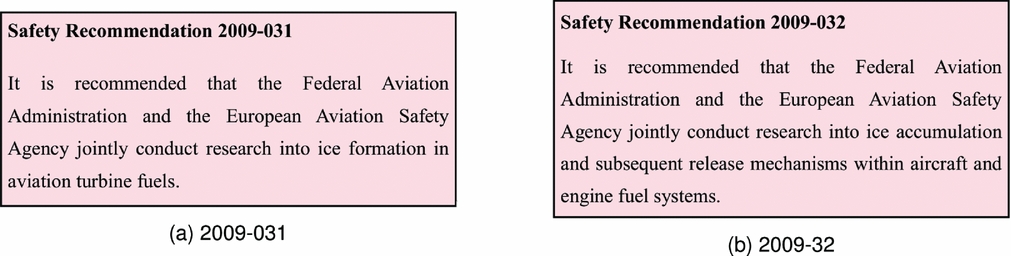
Boeing and Rolls-Royce, under the auspices of the AAIB, conducted fuel system icing tests and research that led the AAIB to establish the cause of the accident. Following the investigation, the AAIB made recommendations towards the European Aviation Safety Agency (EASA) and the Federal Aviation Administration (FAA) for further research into aspects related to water and ice in fuel. Amongst the AAIB safety recommendations, the Safety Recommendation 2009-031 (Fig. 1(a)) was made to address the lack of understanding on how ice forms in jet fuel and the properties of this ice(2). EASA responded to this safety recommendation with a research project titled “Water in aviation fuel under cold temperature conditions (WAFCOLT)” in 2010(9). The project was led by Airbus with academic research support from Cranfield University. Findings from the research project were disseminated to the public in two technical papers(Reference Lam, Carpenter, Williams and Hetherington10,Reference Lam, Lao, Hammond and Power11) .
AAIB safety recommendations.

EASA launched a second research project titled “Ice accretion and release in fuel systems (ICAR)” in 2012 in response to the Safety Recommendation 2009-032 (12). The recommendation (Fig. 1(b)) was made to address the lack of understanding on how ice accumulates and releases within aircraft and engine fuel systems(2). The project was led by Airbus with specialist systems support from Woodford Engineering Consultancy. It is the subject of this technical paper.
1.3 Basis for the ICAR project
Following the Boeing event at Heathrow in 2008, the certification authorities required Boeing, Airbus, and Rolls-Royce to conduct analysis and tests of the aircraft and engine fuel systems on their B777, A330-200/300 and A340-500/600. These tests involved the investigation of factors affecting the accretion of ice in fuel systems, the characteristics of how accumulations of ice may be released and delivered to the engine fuel system and the associated behaviour of the engine fuel system during an ice release event. Further to the A330/A340 family aircraft fuel system icing rig test programme, Airbus has been required to conduct further fuel system icing investigations for A400M, A350, and A320neo aircraft programmes.
Airbus and Woodford Engineering Consultancy have amassed considerable knowledge of fuel systems icing behaviour from these investigations. The experience and the test data gained from all these activities were distilled and released by Airbus to the EASA ICAR project for research and analysis. This paper reports on the key findings of the project. In particular, independent post-project supplemental analysis on accreted ice permeability and interface shear strength are added to the paper for completeness. The discussions on porosity and permeability are limited to accreted ice found in the fuel pipes in the aircraft fuel system prior to the ice release event.
2.0 TEST RIG SET-UP
The Airbus aircraft fuel system icing test programmes were spread over 5 years during which Airbus has undertaken over 260 large-scale ice accretion and release tests. Table 1 shows the test rigs used. The test equipment was initially a relatively simple test section of aircraft fuel pipe. With increasing test experience, the test equipment subsequently progressed up to almost the entire aircraft engine feed system that utilised representative fuel tank structure, fuel tank and engine feed system equipment between the fuel tank boost pump to the engine low-pressure pump inlet. The requirement was to determine the magnitude of the potential icing threat to the engine fuel system so that the engine manufacturer could demonstrate the tolerance of the engine to the threat. The icing threat can be defined as the potential volume of ice that could be released from the aircraft fuel system and delivered to the engine over a specified time period.
Aircraft fuel system icing rigs

Initial icing tests were conducted using the preliminary rig. This was the first occasion when Airbus replicated the type of ice accretions observed by Boeing during the B777 accident investigation. The preliminary rig was used to:
• Identify the important fuel icing test conditions;
• Gain a basic understanding of the effects of the fundamental conditions on ice accretion; and
• Grow experience and confidence with the test methods.
The preliminary rig experience subsequently drove the development of the ice accretion/release rig, providing a platform for testing at a greater level of refinement in terms of test equipment complexity and control, and developed into a test campaign, during which a wider range of conditions was investigated.
Table 2 provides a general overview of the operating conditions across all rigs. Specific operating conditions may vary from rig to rig and from test to test. Each operating parameter was examined in turn to determine the worst-case condition. This condition would be used in subsequent tests of each operating parameter until all worst-case conditions were determined. The final set of worst-case conditions represented an unlikely combination of real aircraft conditions, but ensured, as far as reasonably practicable, a worst possible icing threat level. It was not feasible within the scope and time available to make exhaustive trend analysis investigations of each operating parameter and to establish how all combinations of the different operating parameters affected ice accretion and release levels.
General operating conditions across all rigs

2.1 Accretion tests
All three test rigs in Table 1 were designed for ice accretion tests. The operation of the preliminary rig for ice accretion tests is described in this section. Other test rigs were operated in a similar fashion for ice accretion tests.
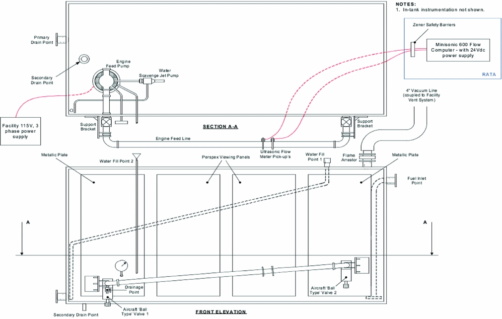
Figure 2 shows the schematic of the preliminary rig. The rig comprised a conditioning tank and a test element. The conditioning tank incorporated cooling radiators built into the tank floor and top cover, which were cooled by a proprietary coolant fluid that enabled the fuel tank to be cooled, at aircraft rates of cooling, to fuel temperatures as low as - $\mathrm{40\; \mathrm{\mathrm{^{\circ }}\mathrm{\mathrm{C}}}}$. The conditioning tank was fitted with an engine feed pump mounted on the tank floor. The pump delivered fuel via a simulated engine feed line and to a fuel system water scavenge jet pump. The water scavenge jet pump facilitated the dispersal and mixing of de-ionised water added in specific quantities to the conditioning tank. The engine feed line exited the conditioning tank and connected to an external pipework. The external pipework consisted of a test element constructed from aircraft fuel system pipework,
 $\mathrm{63.5\;\mathrm{m}\mathrm{m}}$ (2.5 in) diameter ×
 $\mathrm{880\;\mathrm{m}\mathrm{m}}$ length (see “Pipe diameter” in Table 2 for further information), two shut-off valves, an ultrasonic flow meter and other instrumentation. The external fuel pipe was encapsulated in an insulated shroud pipe that was filled with cold fuel from the conditioning tank to simulate the fuel tank environment. The pipework was installed externally to enable inspection of the engine feed line ice accretions post-test.
Schematic of the preliminary rig.

The rig was cleaned and dried prior to the introduction of the test fuel. It was purged by blowing through a dry air of less than 10% relative humidity for 30 minutes. It was then filled with Jet A-1 fuel taken from the test facility fuel storage. The same batch of fuel was used throughout the test campaign to eliminate potential inconsistencies in the test results due to the variation of fuel constituents. The rig was freely vented to ambient during filling.
After filling, the fuel was “sparged” or aerated to ensure the fuel had consistent aeration level (see “Fuel aeration” in Table 2 for further information). When the fuel reached the required aeration level, a “U” pipe section in the vent line was filled with fuel to isolate the conditioning tank ullage space to ambient. The engine feed pump was started and fuel was circulated through the test element at  $\mathrm{9,072\;\mathrm{k}\mathrm{g}.\mathrm{h}^{-1}}$ (
 $\mathrm{20,000\;lb.\mathrm{h}^{-1}}$) to facilitate fuel and water mixing. The rig cooling system was set to maintain the fuel at
 $\mathrm{5\; \mathrm{\mathrm{^{\circ }}\mathrm{\mathrm{C}}}}$.
The fuel was sampled and the water content measured using the coulometric Karl Fischer titration process. Based on the initial water contamination level, the required volume of de-ionised water was added to the tank. The water was introduced slowly over a period of several minutes adjacent to the inlet of the engine feed pump. The water was mixed in the tank for at least 30 minutes to ensure a uniform saturation and dispersal of water. Following the addition of water, further fuel samples were taken to ensure that the required water contamination level was attained (see “Initial water concentration” in Table 2 for further information). Further de-ionised water was added if necessary.
Once the requisite water contamination level was attained, the required fuel flow rate was established (see “Accretion fuel flow rate” in Table 2 for further information) and the fuel was cooled to give a specified fuel temperature versus time profile of a typical flight. The fuel continued to flow through the test element throughout the cooling phase so that the fuel pipe was exposed to the water contamination and the changes in fuel temperature as would occur during “normal” aircraft operation. Ice accretion took place predominately at the test element where the ambient temperature was below the engine feed temperature by as much as  $\mathrm{10\; \mathrm{\mathrm{^{\circ }}\mathrm{\mathrm{C}}}}$ (see “Accretion engine fuel feed ambient temperature” in Table 2 for further information). The cold ambient temperature made the pipe wall temperature in the test element cooler than the engine feed temperature which was at -
 $\mathrm{15\; \mathrm{\mathrm{^{\circ }}\mathrm{\mathrm{C}}}}$ (see “Accretion engine fuel feed temperature” in Table 2 for further information). This provided a negative heat flux such that thermal energy flowed from the fuel next to the test element internal wall through the test element wall to the surround fluid – air/fuel (see “Accretion engine fuel feed surround fluid” in Table 2 for further information), next to the test element external wall. It caused accreted ice to form on the test element internal wall.
At the end of the ice accretion test, after the rig had run for the requisite duration (see “Duration of test” in Table 2 for further information), the engine feed pump was stopped and the test element pipe isolated. Fuel inside the test element was drained. The test element was inspected and photographed to record the presence of any ice accretions. The accreted ice in the test element, including any ice in the fuel drained from the test element, was then collected in sampling containers. The samples were sealed immediately after the collection to prevent any water loss from or water gain to the samples from ambient. The samples were allowed to melt in a warm environment. The volume of water was measured and used to quantify the ice accretion.
To determine the accreted ice porosity n, specific selected samples of accreted ice were taken from the test element pipe wall. The samples went through the same process described in the last paragraph. Since the accreted ice was akin to snow, it trapped a lot of fuel in its snow matrix. When melted, the accreted ice would separate out to water and fuel. The volumes of the fuel and water were measured and used to calculate the accreted ice porosity n. Details of the calculation are given in Appendix A.
2.2 Release tests
Of the three test rigs in Table 1, only the ice accretion/release rig had the added capability for ice release tests. Its operation for ice release tests is described in this section.
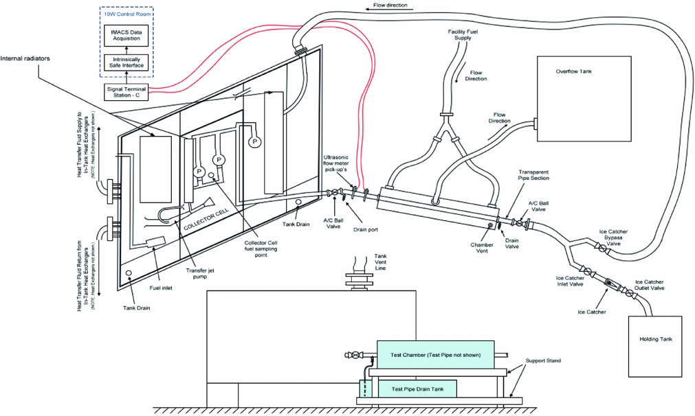
Figure 3 shows the schematic of the ice accretion/release rig. The rig comprised a conditioning tank, a test chamber and an ice catcher. The conditioning tank represented an aircraft wing tank layout, which embodied basic tank structure, including the rear and centre spars, ribs, stringers and a collector cell. The conditioning tank incorporated two engine fuel feed system main pumps and a standby fuel boost pump, a fuel transfer and a fuel system water scavenge architecture. Internal heat exchangers were fully immersed in fuel inside the conditioning tank and enabled the fuel to be cooled to - $\mathrm{40\; \mathrm{\mathrm{^{\circ }}\mathrm{\mathrm{C}}}}$. Thus, as far as possible, the scale of the conditioning tank and the associated aircraft equipment ensured that the movement of fuel and water within the conditioning tank replicated that of the aircraft fuel tank.
Schematic of the ice accretion/release rig.

Fuel was delivered from the conditioning tank to a test element which ran through the test chamber from end-to-end. The test element represented an aircraft engine fuel feed system pipework. The test chamber which encased the test element could be filled with fuel or air to provide two distinctive engine fuel feed surround fluid environments. Both fuel and air were thermally controlled independently of the conditioning tank.
Downstream of the test element, the flow path could be sent in either one of two directions. During accretion tests, fuel flow was recirculated back to the conditioning tank. Based on a nominal cruise fuel flow rate, the fuel volume was re-circulated less than three times during a 6-hour accretion test. During ice release tests, fuel flow was diverted through to an ice catcher and into a separate holding tank located further downstream. The ice catcher, shown in Fig. 4, was a conical wire mesh strainer. It utilised a size 20 (20 holes per inch) round wire bead mesh supported by a gauze of  $\mathrm{3\;\mathrm{m}\mathrm{m}}$ diameter perforations.
Ice catcher.

Ice release tests were initiated immediately after the ice accretion tests by diverting the fuel flow from the conditioning tank return line into the ice catcher and the holding tank. The fuel flow was increased to the specified fuel flow rate at a prescribed rate to simulate the increase in fuel flow demand of the aircraft engine. The release tests were conducted by a delta flow increase, typically from the ice accretion flow rate of  $\mathrm{2,812\;\mathrm{k}\mathrm{g}.\mathrm{h}^{-1}}$ (
 $\mathrm{6,200\;lb.\mathrm{h}^{-1}}$) to the specified ice release flow rate (see Release fuel flow rate in Table 2 for further information). The fuel flow was stopped 2 minutes following the last observed release of ice. The ice catcher was then drained and removed from the rig. It was placed in a sealed container and the ice was allowed to thaw overnight. The meltwater volume from the holding tank and ice catcher was measured to quantify the degree of ice release in terms of ice release percentage χ.
Ice release percentage χ is defined as:
 $$\begin{equation}
\chi = \frac{m_{rel}}{m_{acc}} \times 100\% = \frac{m_{rel}}{m_{rel} + m_{rem}} \times 100\%
\end{equation}$$
Here, m rel is the mass of the meltwater of the ice caught in the holding tank and ice catcher, m rem is the mass of the meltwater of the ice left in the test element, and m acc = m rel + m rem is the mass of the meltwater of the ice accreted in the test. There was a high degree of uncertainty on ice release percentage χ. This was because of the variability inherent in the nature of fuel icing testing. The extent of ice accretion and release was determined from a number of repeat tests using the same final worst-case test conditions and was defined not by the average volume of ice released, but from the maximum level of icing obtained during testing.
3.0 RESULTS AND DISCUSSION
3.1 Accretion levels
Icing investigations conducted with test elements consisting of straight and curvilinear fuel pipe sections established that ice accretion was non-uniform within the engine fuel feed pipework. Accretion levels were not uniformly distributed in longitudinal or circumferential directions. Accretion thickness for most parts were found to be about  $\mathrm{2\;\mathrm{m}\mathrm{m}}$, however, ice thickness in some parts was up to
 $\mathrm{5\;\mathrm{m}\mathrm{m}}$. Observations showed that local accretion levels could be dependent on a number of factors, including, among others, flow regime within the pipework.
3.2 Porosity
Analysis of the character of the accreted ice collected from the accretion tests showed the ice was very porous. Table 3 shows the porosity n of accreted ice from Airbus icing investigations and data from published literature. Although the data shows that there was a large variability of accreted ice porosity n, which ranged from 0.51 to 0.95, the variable range was similar to that of freshly fallen atmospheric snow. Measurements of freshly fallen snow in the atmosphere may vary with snow-to-liquid ratio (SLR) ranging from 3 to 100(Reference Roebber, Bruening, Schultz and Cortinas13-Reference Ware, Schultz, Brooks, Roebber and Bruening16), or porosity n from 0.64 to 0.99. Porosity n and SLR are two of several parameters commonly used to quantify snow character. Other parameters, such as snow density ρs, water content fraction f w and specify gravity (SG) may be used. Definitions and interrelationships of these parameters are given in Lam et al(Reference Lam, Lao, Hammond and Power11).
Character of accreted ice

The variation of porosity, among other factors, may be attributed to how water was introduced to and mixed with the fuel in the icing investigations. In the aircraft icing investigations, Airbus conducted one set of tests (test series R11) using the injection method and the remaining tests using the standard Airbus method.
Standard Airbus Method A prescribed volume of water was added to and thoroughly mixed with the fuel at ambient temperature at the start of the test procedure. No additional water was introduced once the cooling phase commenced. The fuel and water mixture was chilled slowly at a rate typical of in-service operation. This simulated the rate of the nucleation and growth of ice as it would occur normally during aircraft operation. The procedure described in Section 2.1 circumscribes the Standard Airbus method.
Injection Method The test was conducted without the addition of any free water at the start of the cooling phase. Once the test thermal conditions were established, a prescribed volume of water at a prescribed rate was introduced into the cooled fuel at the inlet of the fuel boost pump strainer. The injection stream broke up into varying sizes of water droplet. The injection of water into cold fuel, resulted in rapid cooling and ice nucleation of the injected water. These water droplets were considered larger than those evolved from dissolved water which were reported to be on the order of
${1 \mu {m}}$(Reference Lam, Hetherington and Carpenter17-Reference Schab19).

The two methods produced ice of distinctly different porosity. It was observed that when water was added to cold fuel in the injection method, this produced finer ice particles which contained a higher water content (i.e. lower porosity), and the ice formed had a different appearance to that formed under the standard Airbus method. The implications on ice accretion levels of the two types of ice were not evaluated, but it was noted that the thermal properties such as specific heat capacity and thermal conductance of the two types of ice would differ in proportion to the differences in the amounts of fuel and water in the accreted ice composition.
Libbrecht(Reference Libbrecht20) noted that snow crystal growth dynamics is typically dominated by attachment kinetics in combination with two transport effects:
• Particle diffusion which carries water molecules to the growing crystal; and
• Heat diffusion which removes latent heat released by solidification.
The broad range of snow crystal morphologies reflects the variety of interactions of these processes. Under the particle diffusion limited condition, snow crystals favoured dendritic growth(Reference Libbrecht20); and under unbounded particle diffusion conditions, snow crystals favoured prism or plate growth(Reference Libbrecht20). The snow crystal growth dynamic in the fuel icing investigation was complex. It was not identified what, why and how the standard Airbus method and the injection method attributed to the snow growth dynamic and thereby the character of the accreted ice in terms of porosity n, interface (adhesive) shear strength τa and internal (cohesive) shear strength τc, and the influence on ice release. Further investigations on the topic are required.
3.3 Permeability
Since the accreted ice was porous and thereby permeable, fuel is able to penetrate and flow through it. Permeability is a measure of the ability of fluids to flow through porous media. High permeability allows fluids to flow through porous media rapidly. It is typically an increasing function of porosity(Reference Costa21-Reference Shimizu24), whereby high porosity generally gives high permeability and vice versa.
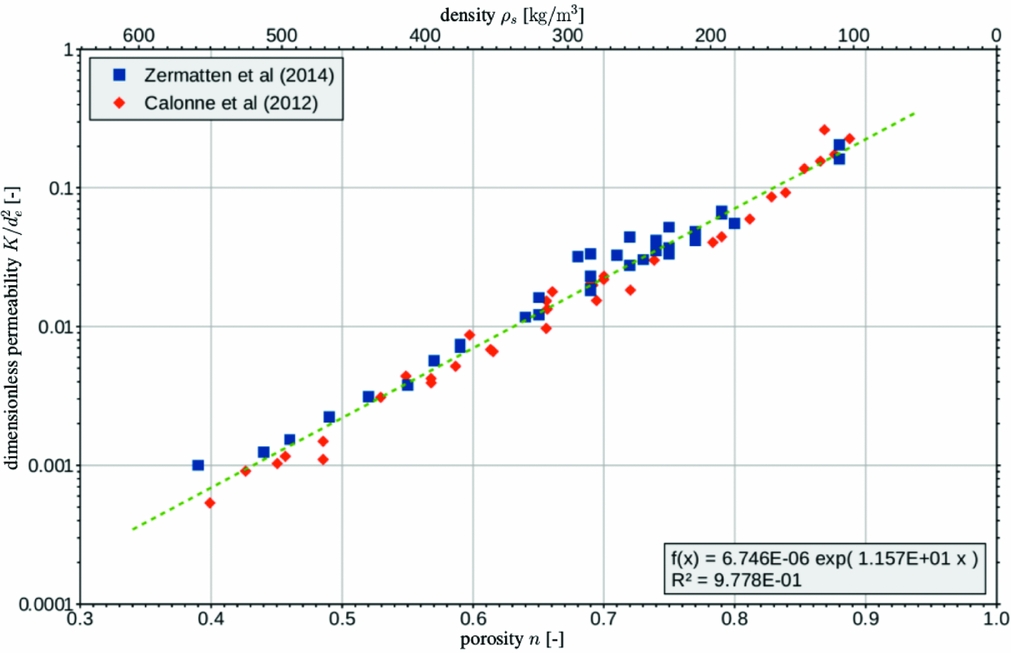
Snow permeability may be determined physically through laboratory tests(Reference Shimizu24) or computationally through tomography(Reference Zermatten, Haussener, Schneebeli and Steinfeld25,Reference Zermatten, Schneebeli, Arakawa and Steinfeld26) . Owing to project constraints, neither method was used in the icing investigations. Instead, the accreted ice permeability was determined with reference to published data and models for freshly fallen snow in the atmosphere. Figure 5 shows the scatter data from Calonne et al(Reference Calonne, Geindreau, Flin, Morin, Lesaffre, Rolland du Roscoat and Charrier27) and Zermatten et al(Reference Zermatten, Schneebeli, Arakawa and Steinfeld26) on a dimensionless permeability K/d 2e versus porosity n plot. Here, K and d e are the permeability and the equivalent grain diameter, respectively. The data exhibit a good correlation between dimensionless permeability K/d 2e and porosity n, and the best fit line to the data is given by:
 $$\begin{equation}
\frac{K_{Cal-Zer}}{d_{e}^{2}} = 6.746 \times 10^{-6} \, \exp (11.57 \, n)
\end{equation}$$
Table 4 summarises a number of permeability correlation models from the literature together with the current model K Cal − Zer derived with the data from Calonne et al(Reference Calonne, Geindreau, Flin, Morin, Lesaffre, Rolland du Roscoat and Charrier27) and Zermatten et al(Reference Zermatten, Schneebeli, Arakawa and Steinfeld26). For direct comparison, all correlation models in the table are expressed in terms of the snow density ρs. The interrelationship of porosity n and snow density ρs is given as(Reference Lam, Lao, Hammond and Power11):
 $$\begin{equation}
n = 1 - \frac{\rho _{s}}{\rho _{i}}
\end{equation}$$
Here,  $\rho _{i} = \mathrm{916.7\;\mathrm{\mathrm{\mathrm{k}\mathrm{g}}.\mathrm{\mathrm{m}}^{\mathrm{-3}}}}$ is the ice density.
Dimensionless permeability K/d 2e as a function of snow porosity n.

Comparison of permeability correlation models

ρs = ρi (1 − n) is the snow density;  $\rho _{i} = \mathrm{916.7\;\mathrm{\mathrm{\mathrm{k}\mathrm{g}}.\mathrm{\mathrm{m}}^{\mathrm{-3}}}}$ is the ice density.
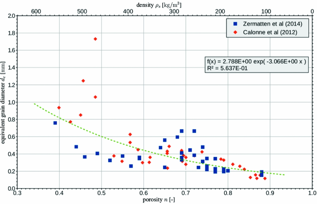
Figure 6 shows equivalent grain diameter d e plotted against porosity n with data from Calonne et al(Reference Calonne, Geindreau, Flin, Morin, Lesaffre, Rolland du Roscoat and Charrier27) and Zermatten et al(Reference Zermatten, Schneebeli, Arakawa and Steinfeld26) (i.e. the same data source as used in Fig. 5). The figure shows a wide data scatter indicating a poor correlation between equivalent grain diameter d e and porosity n. Nevertheless, a general trend may be picked out which gives:
 $$\begin{equation}
d_{e} = 2.788 \times 10^{-3} \, \exp (-3.066 \, n)
\end{equation}$$
The equivalent grain diameter d e, as put forward by Equation (4), decreases exponentially with increasing porosity n. Substituting Equation (4) into Equation (2) and simplifying gives:
 $$\begin{equation}
K_{Cal-Zer} = 5.244 \times 10^{-11} \, \exp (5.438 \, n)
\end{equation}$$
The accreted ice permeability is estimated to be  $\mathrm{7.0\times 10^{-9}\;\mathrm{\mathrm{\mathrm{m}}^{\mathrm{2}}}}$ from Equation (5) with a typical porosity n of 0.9 from the standard Airbus icing tests (Table 3). To gain some perspective, it should be noted that the snow permeability is comparable to that of sandy gravel(28).
Equivalent grain diameter d e as a function of snow porosity n.

3.4 Ice release mechanisms
A number of mechanisms are in play in ice release. The complete mechanisms and underlying physics of ice release are far too complex to undertake in this study. The observations below were filmed and found to be frequent occurrences which sometimes resulted in gradual loss of ice accretions before the planned ice release run:
Shear Release Fluid dynamic shear force overcame the interface shear strength bonding the accreted ice to the internal pipe wall. The flow lifted off the accreted ice from the wall and released it to the flow stream. This was the predominant ice release process that led to the worst-case ice threat delivered to the engine fuel system.
Fracture Release Released ice from upstream collided with the accreted ice on the pipe wall downstream. The collisions caused localised fragments of accreted ice to be broken off from the wall to the flow stream.
Avalanche Release Released ice from upstream was pushed up against the accreted ice on the pipe wall downstream. When sufficient fluid dynamic force had built up behind the arresting ice mass, a sudden localised flush of ice mass was washed downstream.
It was established that the worst-case ice release events occurred when there was a sudden large increase in fuel flow. In a flight operation, a sudden large increase of fuel flow would arise, for example, when full engine power fuel flows are required to undertake a go-around on approach. The worst-case ice release event is defined at take-off and go around (TOGA) fuel flows, when more than 90% of the accreted ice is released simultaneously. The ice release phenomena may be compared to a train leaving a station platform. Testing also showed that smaller quantities of ice may be released by changes in fuel flow rate, e.g. flow cycling from cruise fuel flow to flight idle fuel flow and back to cruise fuel flow resulted in ice being released.
3.5 Interface shear strength
An idealised model with reduced complexity has been proposed as a surrogate model to get a rough order of magnitude of the interface shear strength adhering the accreted ice to the internal pipe wall. The model was a simple pipe flow with porous wall lining computational fluid dynamics (CFD) model. It assumed a fully developed fuel flow in a pipe with a layer of accreted ice modelled as a porous medium on the internal pipe wall. To keep the model simple, the ice accretion was assumed to be uniform with a finite constant thickness throughout the pipe. Ice release may be correlated to the fluid dynamic shear force of the fuel flow if it was acted by the shear release mechanism only.
A number of studies on fluid flows over and within a porous medium have been reported(Reference Suga and Nishio29-Reference Breugem and Boersma41). Experiments and numerical simulations have shown that the flow penetrates into the porous medium in the interface region. The slip velocity at the porous-fluid interface can be considerably greater than the mean bulk velocity within the body of the porous medium. The flow interaction with the porous medium was complex and lent itself to CFD for the determination of stream-wise pressure gradient. Details of the CFD modelling are summarised in Appendix B.
The relationship between wall shear stress and pressure gradient in a simple pipe flow is summarised in Appendix C. Applying the same principle in a pipe flow with porous wall lining, the stream-wise pressure gradient is caused by the shear stress at the porous-fluid interface, at the body of the porous medium and at the pipe wall. From the pressure gradient, an equivalent wall shear stress τw may be calculated for a pipe flow with porous wall lining using Equation (12). This equivalent wall shear stress τw is an approximation to the shear stress acting on the porous medium.
Since most parts of the engine fuel feed pipework were covered with accreted ice of around  $\mathrm{2\;\mathrm{m}\mathrm{m}}$ thick (refer to Section 3.1), a porous lining thickness close to that for the CFD model was desirable. With the porous lining thickness going up in discrete steps due to the discrete nature of the CFD grid, the porous lining thickness of
 $\mathrm{2.1671\;\mathrm{m}\mathrm{m}}$ was found to be the most applicable one to use for the CFD model. Table 5 shows the equivalent wall shear stress for the pipe flow with
 $\mathrm{2.1671\;\mathrm{m}\mathrm{m}}$ thick porous wall lining of porosity 0.90 in a pipe of internal diameter
 $\mathrm{60.20\;\mathrm{m}\mathrm{m}}$ at three arbitrary fuel flow rates. The internal diameter
 $\mathrm{60.20\;\mathrm{m}\mathrm{m}}$ was a typical internal diameter of a
 $\mathrm{63.5\;\mathrm{m}\mathrm{m}}$ (2.5 in) diameter engine fuel feed pipe which was used on Airbus aircraft. The porosity, n = 0.90, represented a typical porosity from the standard Airbus icing tests (Table 3). Lengthwise pressure gradients were yielded from the CFD analysis and converted to equivalent wall shear stresses using Equation (12). The specifications for the pipe flow CFD model with porous wall lining were to simulate the fuel flow in engine feed pipe of the icing investigations. Further details of the CFD analysis can be found in Appendix D.
Equivalent wall shear stress τw for pipe flow with porous wall lining of porosity n = 0.90 and porous lining thickness t = 2.1671 mm at various fuel flow rates

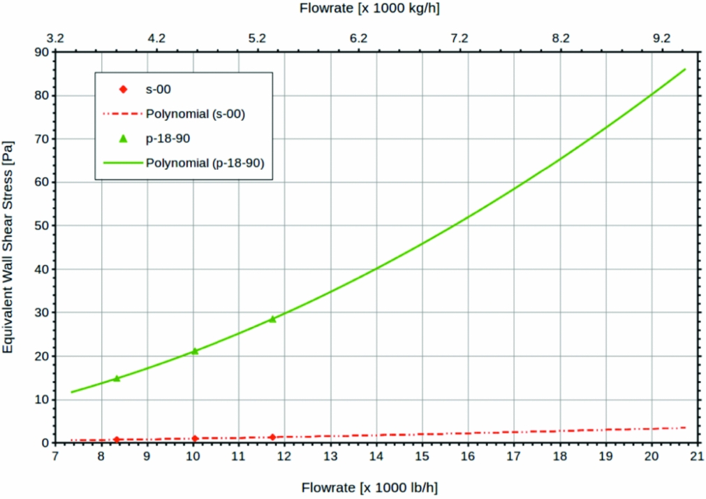
Figure 7 shows the correlation between mass flow rate and equivalent wall shear stress for fuel flow in a pipe with porous lining from the CFD analysis. The mass flow rate and equivalent wall shear stress showed a weak quadratic correlation. Two sets of data are presented. They are:
p-18-90 This denotes a model with a porous wall lining of a uniform thickness
$t = \mathrm{2.1671\;\mathrm{m}\mathrm{m}}$ with a porosity n = 0.90. Data as per tabulated in Table 5.s-00 This denotes a model with no porous wall lining, i.e. zero accreted ice thickness. This represents a simple pipe flow and serves as a reference datum.

Correlation between mass flow rate and equivalent wall shear stress for pipe flow models p-18-90 and s-00.

Table 6 shows the ice release flow rates and their corresponding ice release percentages χ and equivalent wall shear stresses τw. Three fuel flow rates were investigated for ice release. The ice release flow rate and its corresponding ice release percentage χ data are from ice release investigation with  $\mathrm{63.5\;\mathrm{m}\mathrm{m}}$ (2.5 in) diameter pipework. The investigation was part of a certification programme with only a small number of ice release tests. More data points would be desirable. The equivalent wall shear stress values are look-up values from Fig. 7.
Ice release fuel flow rates and their corresponding ice release percentages χ and equivalent wall shear stresses τw

In order to get a rough order of magnitude of the interface shear strength adhering the accreted ice to the internal pipe wall, it is assumed the ice release is strictly shear release. At a low ice release flow rate,  $\mathrm{4,082\;\mathrm{k}\mathrm{g}.\mathrm{h}^{-1}}$ (
 $\mathrm{9,000\;lb.\mathrm{h}^{-1}}$), the equivalent wall shear stress is
 $\mathrm{17.2\;\mathrm{Pa}}$. At this flow rate, accreted ice with interface shear strength of less than
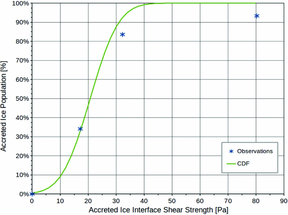
 $\mathrm{17.2\;\mathrm{Pa}}$ would be sheared off from the internal pipe wall and entrained in the fuel delivered to the ice catcher. Since the ice release percentage is 34.08%, this suggests that 34.08% of the accreted ice has interface shear strength less than
 $\mathrm{17.2\;\mathrm{Pa}}$. Similarly, from the results for intermediate and high ice release flow rates, it may be deduced that 83.59% and 93.32% of the accreted ice has interface shear strength less than
 $\mathrm{32.3\;\mathrm{Pa}}$ and
 $\mathrm{80.3\;\mathrm{Pa}}$, respectively.
The trend of the data suggested that the accreted ice interface shear strength did not have a unique value. Accreted ice with low or weak interface shear strength was flushed out at low fuel flow rates, and ice with high or strong interface shear strength at high fuel flow rates. The accreted ice interface shear strength varied over a range of values depending on the local conditions, including, among others, nucleation and initial growth of the accreted ice, and the random nature of the accreted ice conglomerations prior to the release event.
If the accreted ice interface shear strength is a random variable with a normal (Gaussian) distribution, a cumulative distribution function (CDF) Φ for the accreted ice interface shear strength τa may be fitted to the data to quantify the trend (Fig. 8). For a general normal distribution with mean μ and deviation σ, the CDF Φ is given by:
 $$\begin{equation}
\Phi \left( \frac{\tau _{a} - \mu }{\sigma } \right) = \frac{1}{2} \left[ 1 + \mbox{erf}\left( \frac{\tau _{a} - \mu }{\sigma \, \sqrt{2}} \right) \right]
\end{equation}$$
Mean μ and deviation σ were found to be  $\mathrm{20.7\;\mathrm{Pa}}$ and
 $\mathrm{8.0\;\mathrm{Pa}}$ by non-linear least squares regression fitting the three data points from Table 6. The regression fitting also needed to satisfy the requirement that accreted ice cannot have a negative interface shear strength, i.e. τa > 0. This implies that the fitted curve must pass through the point (0, 0). From the CDF Φ, the lower (or first) quartile Q 1, the upper (or third) quartile Q 3 are:
 $$\begin{equation}
Q_{1} = \mu - 0.6745\, \sigma = \mathrm{15.3\;\mathrm{Pa}}
\end{equation}$$
 $$\begin{equation}
Q_{3} = \mu + 0.6745\, \sigma = \mathrm{26.1\;\mathrm{Pa}}
\end{equation}$$
 $\mathrm{15.3\;\mathrm{Pa}}$,
 $\mathrm{20.7\;\mathrm{Pa}}$ and
 $\mathrm{26.1\;\mathrm{Pa}}$, respectively, and 50% of the accreted ice has interface shear strength in the interquartile range between
 $\mathrm{15.3\;\mathrm{Pa}}$ and
 $\mathrm{26.1\;\mathrm{Pa}}$.
Cumulative distribution function (CDF) Φ for the accreted ice interface shear strength τa.

4.0 CONCLUSIONS
An overview of the Airbus ice accretion and release tests within the scope of EASA ICAR project was given with brief narratives on the test rigs, the test procedure and methodology. Key findings from the icing investigations were presented. Further to the EASA ICAR project, supplemental analysis on accreted ice permeability and interface shear strength were included for completeness. From the icing investigations for fuel flow in  $\mathrm{63.5\;\mathrm{m}\mathrm{m}}$ (2.5 in) diameter engine fuel feed pipes, the data and the analysis showed:
• The porosity of the accreted ice was c. 0.90.
• The permeability of the accreted ice was found to be c.
$\mathrm{7.0\times 10^{-9}\;\mathrm{\mathrm{\mathrm{m}}^{\mathrm{2}}}}$.• The accreted ice thickness was non-uniform, however, it is found typically c.
$\mathrm{2\;\mathrm{m}\mathrm{m}}$ thick.• 25% of accreted ice has interface shear strength up to
$\mathrm{15.3\;\mathrm{Pa}}$.• 50% of accreted ice has interface shear strength up to
$\mathrm{20.7\;\mathrm{Pa}}$.• 75% of accreted ice has interface shear strength up to
$\mathrm{26.1\;\mathrm{Pa}}$.


ACKNOWLEDGEMENTS
This work formed part of a European Aviation Safety Agency (EASA) funded research project titled “Ice accretion and release in fuel systems (ICAR)”. The authors wish to thank Airbus Operations Limited for releasing the aircraft fuel system icing rig test data to the project for research and analysis.
APPENDIX A: POROSITY
Porosity n is defined as(Reference Lam, Carpenter, Williams and Hetherington10):
 $$\begin{equation}
n = \frac{\mbox{pore volume}}{\mbox{snow volume}} = \frac{V_{p}}{V_{s}} = \frac{V_{s} - V_{i}}{V_{s}}
\end{equation}$$
Here, V p is the pore volume; V s is the accreted ice volume, or the snow volume; and V i is the solid ice volume. Accreted ice samples, when melted, would separate out to water and fuel. The snow volume V s and the solid ice volume V i may be approximated in terms of water volume V w and fuel volume V f as:
 $$\begin{equation}
V_{s} \approx V_{f} + V_{w}
\end{equation}$$
 $$\begin{equation}
V_{i} \approx V_{w}
\end{equation}$$
 $$\begin{equation*}
n = \frac{V_{f}}{V_{f} + V_{w}}
\end{equation*}$$
The water volume V w and the fuel volume V f may be measured directly with appropriate measuring vessels. Alternatively, they may be determined indirectly from their masses with appropriate densities to convert the masses to volumes.
APPENDIX B: CFD MODELLING
A number of CFD simulations were performed to yield the stream-wise pressure gradients for fully developed steady fuel flow in a pipe of internal diameter  $\mathrm{60.1980\;\mathrm{m}\mathrm{m}}$, i.e. a nominal
 $\mathrm{63.5\;\mathrm{m}\mathrm{m}}$ (2.5 in) outer diameter pipe. The pipe was lined with a layer of porous medium representing the accreted ice at the internal pipe wall of various thickness and porosity. Figure 9 shows the schematic of the model geometry. A two-dimensional axis-symmetric modelling domain with translational periodic boundary condition was used by taking advantage of the model geometry. A structured mesh of 30,000 quadrilateral cells was deployed with 60 cells in the axial direction and 500 cells in the radial direction. Mesh was distributed uniformly in the radial direction, but distributed in a bell-shaped profile in the axial direction with fine mesh at the ends and coarse mesh at the centre. The meshing strategy covered the modelling domain in an efficient way in terms of cell number and solution accuracy.
A schematic of the CFD model geometry.

The translational periodic boundary condition allowed fully developed flow to be modelled with a shortened modelling domain and reduced computational effort. The pair of periodic boundary planes, upstream periodic boundary plane and downstream periodic boundary plane, spanned across two model regions, the porous region and the clear fluid region. Due to limitations of the CFD software application tool, the pair of periodic boundary planes was divided into two sub-pairs of periodic boundary planes, one sub-pair for the porous region and the other sub-pair for the clear fluid region. Although the fuel mass flow rate through the pipe was known, the distribution of the mass flow rates through the clear fluid and porous regions was not known. This caused complication and difficulty in defining the fuel mass flow rates for the two sub-pairs of periodic boundary planes.
A workaround to the dilemma was to keep the porous region away from the periodic boundary planes. The insert in Fig. 9 shows a small gap of just one cell separating the porous region from the downstream periodic boundary plane. A similar arrangement was made at the upstream end. The gaps were incorporated into the clear fluid region as one region, and were kept as small as possible to minimise any impact on the fluid dynamics. Since the pair of periodic boundary planes now spanned across the clear fluid region only, it did not need to split into two sub-pairs of periodic boundary planes as in the default case. The mass flow rate through the pipe was all that needed to specify the boundary condition for the pair of periodic boundary planes.
Model sensitivity to the workaround was assessed to see its impact on solution accuracy. A pipe with an internal diameter  $D = \mathrm{60.1980\;\mathrm{m}\mathrm{m}}$ and a fuel flow rate
 $\mathrm{4,552\;\mathrm{k}\mathrm{g}.\mathrm{h}^{-1}}$ (
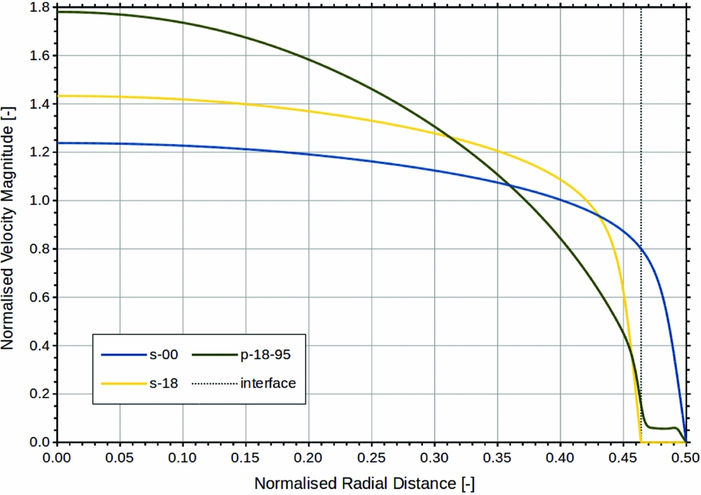
 $\mathrm{10,035\;lb.\mathrm{h}^{-1}}$) was considered. A key parameter to assess was the pressure gradient. Since an empirical equation for pressure gradient for simple pipe flow was available to serve as a benchmark, a special scenario was adapted for the assessment whereby the porous wall lining was replaced with a solid wall lining. The solid wall lining of thickness t, being impermeable, effectively reconfigured the pipe with internal diameter D to a smaller pipe with internal diameter D − 2 t. Table 7 shows a comparison of the pressure gradients computed from the CFD and those calculated from the Darcy-Weisbach equation (Equation (13)). Figure 10 shows the velocity profiles of the two model runs, s-00 and s-18. Further details regarding the model runs are given in Appendix D.
Velocity profiles for simple pipe flow and pipe flow with porous medium wall lining.

Comparison of pressure gradient predictions between the CFD model and the Darcy-Weisbach equation (Equation (13)) for fuel flow rate 4,552 kg.h−1 (10,035 lb.h−1)

The first case, s-00, with no solid wall lining, i.e.  $t = \mathrm{0\;\mathrm{m}\mathrm{m}}$, served as the baseline. The workaround was not applicable in this case and the model was simply a smooth pipe. The table showed that the pressure gradient derived from the CFD simulation was in close agreement with that calculated from the Darcy-Weisbach equation (Equation (13)) with a deviation of 2.03 Pa.m−1 or 3%. This was well within the precision range for the Darcy-Weisbach equation using the Darcy friction factor from the Colebrook-White equation (refer to Table 8). It gave confidence that the model and the solver were set up appropriately for the application.
Darcy friction factor equations

In the second case, s-18, the solid wall lining has a finite thickness,  $t = \mathrm{2.1671\;\mathrm{m}\mathrm{m}}$. With the workaround, this gave rise to a pipe with annular grooves at a regular interval. In addition to the pipe wall friction loss, the flow also incurred additional pressure loss from flow disturbance due to the discontinuity in the solid wall lining. Nevertheless, the CFD result was in close agreement with the benchmark Darcy-Weisbach equation (Equation (13)) with a deviation of 2.19 Pa.m−1 or 2%. This indicates the impact of the workaround on the model was insignificant. The additional loss from flow disturbance due to the discontinuity in the solid wall lining was negligible. The workaround was proved to be acceptable for the application.
APPENDIX C: WALL SHEAR STRESS
Derivation of the wall shear stress τw in a pipe flow by performing a simple force balance has been illustrated in a number of fluid mechanics textbooks(Reference Çengel and Cimbala42-Reference Young, Munson, Okiishi and Huebsch47). For a pipe with radius R, the wall shear stress τw is expressed as:
 $$\begin{equation}
\tau _{w} = \frac{\Delta p \, R}{2 \, l}
\end{equation}$$
Here, Δp is the pressure loss over the pipe length l. The pressure loss Δp can be expressed with the Darcy-Weisbach equation(Reference White48,Reference Brown49) :
 $$\begin{equation}
\Delta p = \frac{\lambda \, l \, \rho \, \bar{u}^{2}}{4 \, R}
\end{equation}$$
Here, λ is the Darcy friction factor; ρ is the fluid density; and  $\bar{u}$ is the pipe mean flow velocity. Although the Darcy friction factor λ for pipe flow is most common, be aware of the alternative friction factor called the Fanning friction factor f. The Darcy friction factor λ is a factor of four of the Fanning friction factor f (Reference Çengel and Cimbala42,Reference White48) , i.e. λ = 4 f. Substituting Equation (13) into Equation (12), the wall shear stress τw may be written as:
 $$\begin{equation}
\tau _{w} = \frac{1}{8} \, \lambda \, \rho \, \bar{u}^{2}
\end{equation}$$
The Darcy friction factor λ may be determined from the Moody diagram(Reference Moody50) or from a number of Darcy friction factor relationships that have been developed over the years(Reference White48,Reference Brown49) . Table 8 shows some selected Darcy friction factor equations. Apart from the equation for laminar flow is an explicit equation, the remaining equations are implicit equations. These implicit equations require an iterative solution where convergence to 0.01% typically requires less than seven iterations(Reference Brkić51).
APPENDIX D: PIPE FLOW WITH POROUS WALL LINING
Figure 10 shows computed velocity profiles for simple pipe flow and pipe flow with porous wall lining. The scenarios presented are:
s-00 A pipe of internal diameter
$D = \mathrm{60.1980\;\mathrm{m}\mathrm{m}}$ with no solid or porous wall lining. This gave a case of simple pipe flow. The internal diameter D represented a typical internal diameter of a $\mathrm{63.5\;\mathrm{m}\mathrm{m}}$ (2.5 in) diameter fuel pipe.s-18 A pipe of internal diameter D was lined with a solid (impermeable) wall lining of thickness
$t = \mathrm{2.1671\;\mathrm{m}\mathrm{m}}$. This reduced the scenario to a case of simple pipe flow of pipe internal diameter $D - 2\,t = \mathrm{55.8638\;\mathrm{m}\mathrm{m}}$.p-18-95 A pipe of internal diameter D was lined with a porous wall lining of thickness
$t = \mathrm{2.1671\;\mathrm{m}\mathrm{m}}$ and porosity n = 0.95. This conveyed a proxy model of accreted ice in a fuel pipe. The porosity n = 0.95 represented a typical porosity from the EASA WAFCOLT project (refer to Table 3).


The notation used for the model runs was written as “m-tt-pp”. Here “m” depicts the medium, “s” for solid and “p” for porous; “tt” depicts the medium thickness in CFD cell count; and “pp” depicts the porosity where applicable. The model p-18-95 corresponded to a case with porous wall lining of porosity n = 0.95; and the wall lining was 18 cells thick giving it a thickness t = 2.1671 (=18 × 0.120396) mm. The three model runs were simulated with an arbitrary fuel flow rate of  $\mathrm{4,552\;\mathrm{k}\mathrm{g}.\mathrm{h}^{-1}}$ (
 $\mathrm{10,035\;lb.\mathrm{h}^{-1}}$). Jet fuel physical properties tabulated in Table 9 and permeability from Equation (5) were applied in the CFD simulation.
Typical physical properties of Jet A-1 at −15 °C

The dotted line labelled “interface” in Fig. 10 marks the position of the porous-fluid interface for p-18-95 and the solid-fluid interface for s-18. The interface was at a distance t, i.e. the solid/porous wall lining thickness, from the pipe wall. With a reduced pipe diameter in s-18, the centreline velocity u max and the mean bulk velocity  $\bar{u}$ were higher than those for s-00. Nevertheless, the two velocity profiles were very similar with the velocity profile characteristic ratio
 $\bar{u} / u_{\text{max}}$ of 0.808 and 0.810 for s-00 and s-18, respectively. The velocity profile for p-18-95 has a different outlook to that for s-18. The velocity profile for p-18-95 may be divided into five regions:
• The boundary-layer flow in the porous medium close to the pipe wall.
• The uniform Darcy flow in the porous medium.
• The interface transition flow in the porous medium close to the porous-fluid interface.
• The pseudo boundary-layer flow in the clear fluid region close to the porous-fluid interface.
• The main fluid flow in the clear fluid region.
In the clear fluid region, p-18-95 showed a strong parabolic characteristic compared to that for s-18 which exhibited a typical flat velocity profile for turbulent flow. With a velocity profile characteristic ratio  $\bar{u} / u_{\text{max}}$ of 0.562, the profile in the clear fluid region for p-18-95 was in fact not much dissimilar to the parabolic profile for laminar flow which has a characteristic ratio
 $\bar{u} / u_{\text{max}}$ of 0.500(Reference Lindeburg52). The difference between the velocity profiles in the clear fluid region for p-18-95 and that for s-18 was due to increased drag caused by the exchange of momentum between the clear fluid and the porous medium(Reference Breugem and Boersma36,Reference Chan, Huang, Leu and Lai38,Reference Breugem, Boersma and Uittenbogaard40) . High stream-wise momentum fluid from the clear fluid region may propagate across the porous-fluid interface into the porous medium, and in return, low stream-wise momentum fluid from the porous medium is transported across the porous-fluid interface to the clear fluid region.
Table 10 shows the effect of porous wall lining thickness on the stream-wise pressure gradient. Pressure gradient for simple pipe flow as if the porous wall lining was an impermeable solid was given as a benchmark in the column labelled “Pressure Gradient Equation (13)”. Derivation of Equation (13), the Darcy-Weisbach equation, and other associated equations are given in Appendix C. Using the wall lining thickness  $t = \mathrm{2.1671\;\mathrm{m}\mathrm{m}}$ as an example, the pressure gradient 1,357.97
 $\mathrm{\;\mathrm{Pa}.\mathrm{m}^{-1}}$ under the column “Pressure Gradient CFD” was computed for p-18-95 by the CFD model, and the pressure gradient
 $\mathrm{89.73\;\mathrm{Pa}.\mathrm{m}^{-1}}$ under the column “Pressure Gradient Equation (13)” was computed for s-18 using Equation (13). The column labelled “Pressure Gradient Ratio 3” shows the ratio of these two pressure gradients. The pressure gradient for pipe flow with porous wall lining is significantly higher than that for simple pipe flow. As discussed in the last paragraph, the exchange of momentum through the porous-fluid interface caused a significant increase in Reynold stresses.
Effect of porous wall lining thickness t on pressure gradient for fuel flow rate 4,552 kg.h−1 (10,035 lb.h−1) and porosity n = 0.95

As the lining thickness t increased from  $\mathrm{0.3612\;\mathrm{m}\mathrm{m}}$ to
 $\mathrm{2.1671\;\mathrm{m}\mathrm{m}}$, i.e. a 6-fold increase, the pressure gradient under the column “Pressure Gradient CFD”, increased from
 $\mathrm{92.18\;\mathrm{Pa}.\mathrm{m}^{-1}}$ to 1,357.97
 $\mathrm{\;\mathrm{Pa}.\mathrm{m}^{-1}}$, i.e. 14.73-fold increase. The pressure gradient increased 2.5 (≈14.73/6.00) times faster than the lining thickness increase. In contrast, for the same lining thickness increase, the benchmark pressure gradient, under the column “Pressure Gradient Equation (13)”, increased from
 $\mathrm{66.64\;\mathrm{Pa}.\mathrm{m}^{-1}}$ to
 $\mathrm{89.73\;\mathrm{Pa}.\mathrm{m}^{-1}}$, i.e. a 1.35-fold increase.
Table 11 shows the sensitivity of pressure gradient on the fuel flow rate. As the fuel flow rate increased from 3,780 $\mathrm{\;\mathrm{k}\mathrm{g}.\mathrm{h}^{-1}}$ (8,333
 $\mathrm{\;lb.\mathrm{h}^{-1}}$) to 5,324
 $\mathrm{\;\mathrm{k}\mathrm{g}.\mathrm{h}^{-1}}$ (
 $\mathrm{11,737\;lb.\mathrm{h}^{-1}}$), i.e. a 1.41-fold increase, the pressure gradient, under the column “Pressure Gradient CFD”, increased from
 $\mathrm{953.16\;\mathrm{Pa}.\mathrm{m}^{-1}}$ to
 $\mathrm{1,821.92\;\mathrm{Pa}.\mathrm{m}^{-1}}$, i.e. a 1.91-fold increase. The pressure gradient increased 1.4 (≈1.91/1.41) times faster than the fuel flow rate increase. It is interesting to note that the benchmark pressure gradient, under the column “Pressure Gradient Equation (13)”, increased from
 $\mathrm{64.95\;\mathrm{Pa}.\mathrm{m}^{-1}}$ to
 $\mathrm{117.93\;\mathrm{Pa}.\mathrm{m}^{-1}}$, i.e. a 1.82-fold increase, for the same fuel flow rate increase. In both cases, the order of increase in pressure gradient of 1.91 and 1.82 is very similar.
Effect of fuel flow rate on pressure gradient for model p-18-95 which has porous wall lining thickness t = 2.1671 mm and porosity n = 0.95.

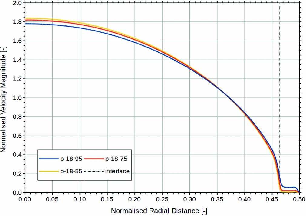
Permeability is an increasing function of porosity (refer to Section 3.3). As the porosity decreases, the permeability decreases and vice versa. The effect of porosity and, hence, permeability on the pressure gradient for fuel flow rate  $\mathrm{4,552\;\mathrm{k}\mathrm{g}.\mathrm{h}^{-1}}$ (
 $\mathrm{10,035\;lb.\mathrm{h}^{-1}}$) is shown in Table 12. As the porosity n decreased from 0.95 to 0.50, the permeability decreased from
 $\mathrm{9.1884 \times 10^{-9}\;\mathrm{\mathrm{\mathrm{m}}^{\mathrm{2}}}}$ to
 $\mathrm{0.7952 \times 10^{-9}\;\mathrm{\mathrm{\mathrm{m}}^{\mathrm{2}}}}$, i.e. a 11.55-fold reduction, and the pressure gradient, under the column “Pressure Gradient CFD”, increased from
 $\mathrm{1,357.97\;\mathrm{Pa}.\mathrm{m}^{-1}}$ to
 $\mathrm{1,634.37\;\mathrm{Pa}.\mathrm{m}^{-1}}$, i.e. a 1.20-fold increase. Although the permeability has decreased by just over an order of magnitude (11.55), the pressure gradient only increased by a relatively small fraction (1.20). This suggests that the pressure gradient is relatively insensitive to permeability. Figure 11 shows the velocity profiles of pipe flow with porous war lining with various porosities and, hence, permeabilities.
Velocity profiles for pipe flow with porous medium wall lining of various porosity.

Effect of porosity on pressure gradient for fuel flow rate 4,552 kg.h−1 (10,035 lb.h−1) and lining thickness t = 2.1671 mm