


1. Introduction
The pioneering aeroacoustics analysis by Lighthill (Reference Lighthill1952) first determined that isolated turbulent eddies in low-speed flows produce sound in a quadrupolar directivity pattern with an intensity that is proportional to  $U^3 M^5$ or
 $U^8$, where
 $U$ and
 $M$ are the characteristic flow speed and Mach number, respectively. The close proximity of turbulence to a solid body amplifies its acoustic intensity and changes the directivity pattern of the scattered sound: Curle (Reference Curle1955) showed that the radiated acoustic power of turbulence scattered by acoustically compact bodies scales on
 $U^6$, which is a factor of
 $M^{-2}$ increase in magnitude for low Mach number flows that is accompanied by a shift to dipolar directivity. Ffowcs Williams & Hall (Reference Ffowcs Williams and Hall1970) examined analytically a more efficient noise generation scenario of turbulent eddies near a non-compact sharp edge, where the acoustic power scales on
 $U^5$, i.e.
 $M^{-3}$ louder than free-field turbulence; a cardioid directivity pattern for pressure accompanies this change in acoustic intensity, which scales on the distance
 $L$ between the turbulent eddy and the edge as
 $L^{-3}$. A sharp edge may be generalised geometrically into a wedge, where Crighton & Leppington (Reference Crighton and Leppington1971) showed that a finite opening angle weakens the acoustic field relative to the
 $U^5$ velocity scaling for classical trailing edge noise.
The efficient conversion of turbulence energy into sound by rigid impermeable edges continues to motivate strategies to disrupt the noise generation process through the modification of trailing edge material properties. Crighton & Leppington (Reference Crighton and Leppington1970) carried out one of the first such analytical investigations by imposing a point-reacting impedance condition on a semi-infinite plate, where in certain parametric limits the plate may be considered as either rigid or limp. The rigid limit recovers the results of Ffowcs Williams & Hall (Reference Ffowcs Williams and Hall1970), and the so-called ‘limp’ edge limit produces a  $U^6$ power scaling and dipolar acoustic field that would be expected for turbulence noise produced by a compact body or a solid body without an edge. More sophisticated models, including flexural waves in a compliant edge, that were not considered by Crighton & Leppington (Reference Crighton and Leppington1970) have since been investigated to study their effect on structural (Crighton Reference Crighton1972a) and aerodynamic (Cannell Reference Cannell1975, Reference Cannell1976; Howe Reference Howe1992, Reference Howe1993a,Reference Howeb, Reference Howe1994), noise, including the influence of structural resonance on radiated sound for finite elastic sections (Leppington Reference Leppington1976; Abrahams Reference Abrahams1981, Reference Abrahams1983).
Porosity is a common design approach to mitigate noise generation that manipulates the edge boundary condition. Ffowcs Williams (Reference Ffowcs Williams1972) determined that turbulence noise from an infinite perforated screen scales on  $U^6$ and has a dipolar directivity in a high-porosity limit, which Nelson (Reference Nelson1982) corroborated experimentally for a porous surface away from its edges. Howe (Reference Howe1979) later examined the sound generation of a vortex passing near a semi-infinite plate with a finite porous extension and showed that the porous section reduces the sound level by relaxing the abrupt change in boundary conditions at the impermeable edge. Kisil & Ayton (Reference Kisil and Ayton2018) constructed an analysis procedure for this configuration and underscored the importance of secondary scattering from the impermeable-porous junction for high-frequency turbulence sources. In addition to these analytical works, the effect of porosity on edge noise reduction has been investigated computationally (Khorrami & Choudhari Reference Khorrami and Choudhari2003) and experimentally (Fink & Bailey Reference Fink and Bailey1980; Geyer, Sarradj & Fritzsche Reference Geyer, Sarradj and Fritzsche2010), and has been reviewed recently by Jaworski & Peake (Reference Jaworski and Peake2020).
Further research attention has been directed towards how the combination of porosity and elasticity reduces turbulence edge noise. Jaworski & Peake (Reference Jaworski and Peake2013) analysed the scaling behaviour of turbulence sound radiated by semi-infinite poroelastic edges using the Wiener–Hopf analysis technique. They recovered the  $U^6$ acoustic power scaling and the dipole directivity results of Ffowcs Williams (Reference Ffowcs Williams1972) in the high-porosity limit for an infinite perforated sheet, indicating that the effect of the edge on the acoustic scaling behaviour is eliminated in this case. In other words, the acoustical non-compactness of an impermeable edge is disrupted by surface porosity, which permits near-field fluid motions through the edge that are associated with an acoustic dipole. Jaworski & Peake (Reference Jaworski and Peake2013) also identified a new
 $U^7$ velocity scaling for elastic edges under specific fluid loading conditions. With the aim to relax the semi-infinite geometrical restriction, Cavalieri, Wolf & Jaworski (Reference Cavalieri, Wolf and Jaworski2016) developed a boundary element method to determine numerically how sound scatters from a finite poroelastic strip. Porosity reduced noise more effectively at low frequencies with wavelengths that are large relative to the strip length, while elasticity was more effective at high-frequency noise reduction. Therefore, poroelasticity may enable broadband noise reduction for finite edge sections or aerofoils. More recent investigations and extensions involving finite geometries include a finite one-dimensional rigid plate with a poroelastic extension (Ayton Reference Ayton2016), multiple finite plates with various material properties (Colbrook & Ayton Reference Colbrook and Ayton2019; Colbrook & Kisil Reference Colbrook and Kisil2020), and generalised two-dimensional poroelastic plates with straight, swept or serrated edges (Pimenta, Wolf & Cavalieri Reference Pimenta, Wolf and Cavalieri2018).
Empirical support provided by Brooks & Hodgson (Reference Brooks and Hodgson1981) and several other measurement campaigns (see Crighton Reference Crighton1991) confirmed the  $U^5$ acoustic power and cardioid directivity predictions by Ffowcs Williams & Hall (Reference Ffowcs Williams and Hall1970) for a rigid and impermeable edge. However, direct experimental confirmation of the
 $U^6$ and
 $U^7$ scalings for highly porous or elastic edges, respectively, is not likely possible in conventional aeroacoustic facilities due to secondary flow noise contributions that may become as loud or louder than the edge noise itself. For example, turbulent boundary layers present on wind tunnel walls and test article surfaces produce roughness noise (Devenport et al. Reference Devenport, Alexander, Glegg and Wang2018) with a dipolar directivity and an intensity that scales on
 $U^6$ (Howe Reference Howe1984). Therefore, the mean flow associated with the turbulent boundary layer that generates edge noise is also a source of acoustic contamination relative to sound produced at porous or elastic edges: in a scaling sense, edge noise in the high-porosity limit would be indistinguishable from roughness noise, which would dominate altogether the weaker
 $U^7$ sound from elastic edges in the appropriate parametric limit.
To circumvent this critical limitation, an alternative approach is proposed using a moving vortex ring as an acoustic source in an otherwise quiescent fluid. The replacement of the turbulence source with a coherent vortex structure is motivated by the seminal analysis of Crighton (Reference Crighton1972b), which determined analytically that a line vortex moving round an edge produces the same  $U^5$ intensity scaling determined by wave scattering analyses (Ffowcs Williams & Hall Reference Ffowcs Williams and Hall1970; Crighton & Leppington Reference Crighton and Leppington1970), where
 $U$ is the vortex ring speed in this configuration. The matched asymptotic results by Crighton (Reference Crighton1972b) were examined further and verified by Howe (Reference Howe1975) using a low-frequency Green's function, and by Möhring (Reference Möhring1978) using a vector Green's function. Kambe, Minota & Ikushima (Reference Kambe, Minota and Ikushima1985) validated the vortex sound approach by achieving the
 $U^5$ intensity scaling using a vortex ring shot rectlinearly past a rigid impermeable edge, and confirmed its cardioid directivity. Their analysis of vortex ring sound obtained an
 $L^{-4}$ intensity scaling based on the minimum distance between the vortex path and the edge, which is distinct from the scaling of Ffowcs Williams & Hall (Reference Ffowcs Williams and Hall1970) for turbulence scattering and is particular to the vortex ring configuration. Crucially, the vortex ring configuration of Kambe et al. (Reference Kambe, Minota and Ikushima1985) does not require a background mean flow and therefore does not introduce flow noise sources that would potentially corrupt an acoustic measurement of the edge noise emission.
A theoretical–experimental campaign is reported here in two parts and uses the vortex ring approach to measure directly the sound that it generates near a porous edge, which aims to confirm by analogue the analytical predictions of Jaworski & Peake (Reference Jaworski and Peake2013). Part 1 describes the theoretical model against which measurements in Part 2 are compared, and the remainder of this part is organised as follows. Section 2 describes the vortex sound model and constructs the associated Green's function to estimate the acoustic emission of a vortex ring passing near a porous edge. This analysis takes the approach of Kambe et al. (Reference Kambe, Minota and Ikushima1985) used for an impermeable plate, and extends the results of Jaworski & Peake (Reference Jaworski and Peake2013) for a porous plate to a vortex sound context. Section 3 discusses results from the mathematical model, including the parametric limits of low and high porosity and their influence on the directivity and acoustic intensity scaling behaviours. Conclusions and final remarks are presented in § 4.
2. Mathematical model
2.1. Vortex sound at low Mach numbers
Consider a rigid semi-infinite porous plate with negligible thickness that lies in the region  $-\infty < x_1,y_1\leq 0$,
 $x_2,y_2=0$,
 $-\infty < x_3,y_3<\infty$ of the coincident Cartesian coordinate systems {
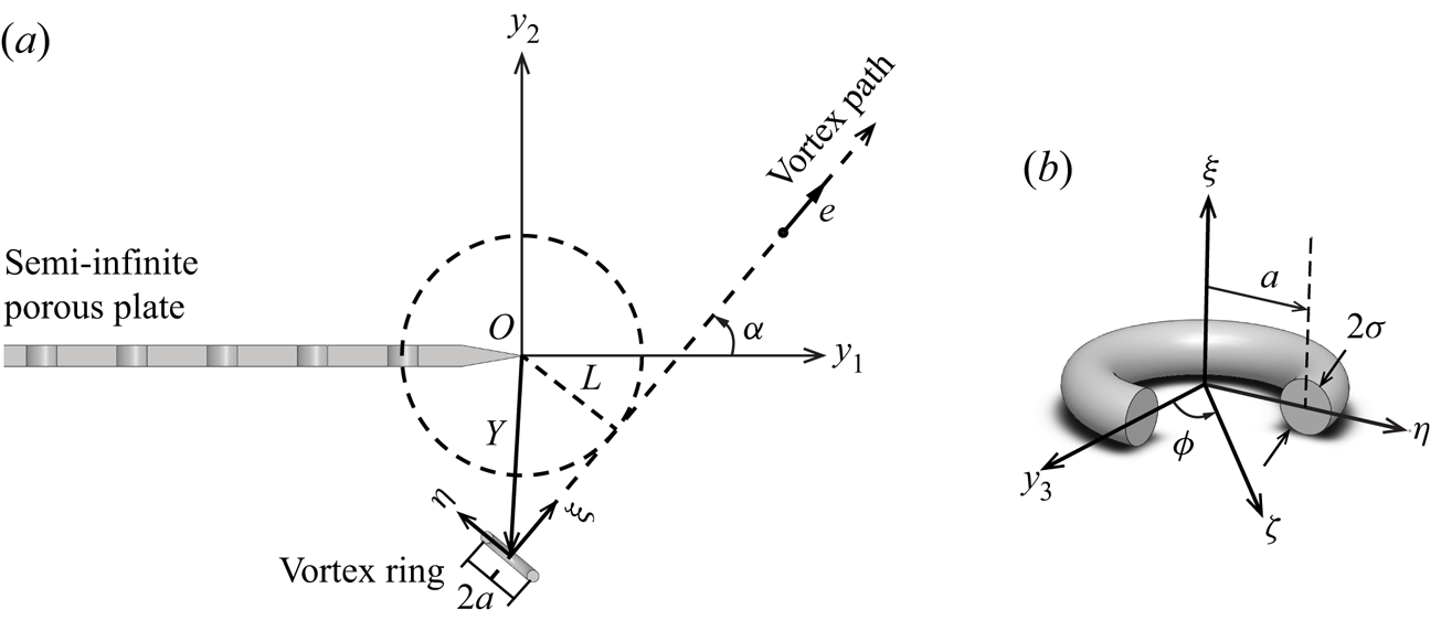
 $(x_1,y_1), (x_2,y_2), (x_3,y_3)$}, as shown in figure 1. The porous plate is immersed in an unbounded fluid at rest at infinity. The present work studies the acoustic emission by an acoustically compact vortex ring source passing near the edge of a porous half plane. Source compactness requires
 $l/\lambda \ll 1$, where
 $l$ is the length scale of the turbulent source, and
 $\lambda$ is the wavelength of the emitted sound. The Mach number
 $M$, defined by
 $U/c$, is assumed to be much smaller than unity, where
 $U$ is the characteristic speed of the vortex ring and
 $c$ is the sound speed.
Schematic of the porous half-plane and the coincident coordinate systems for the compact vortex ring source  $\boldsymbol {y} = (\kern 0.05em y_1, y_2, y_3)$ and the observer at
 $\boldsymbol {x} = (x_1, x_2, x_3)$.

The sound resulting from the vortex ring interaction with the porous edge may be described by the inhomogeneous wave equation forced by the Lamb vector (Howe Reference Howe1998, p. 188),
 \begin{equation} \left(\frac{1}{c^2}\,{\frac{\partial^2{}}{\partial{t}^2}}-\nabla^2\right) p = \rho\,{\rm{div}}(\boldsymbol{\omega} \times \boldsymbol{v}), \end{equation}
which admits a general solution in terms of a boundary integral,
 \begin{equation} p(\boldsymbol{x},t)={-}\rho \iint (\boldsymbol{\omega} \times \boldsymbol{v})(\kern 0.06em \boldsymbol{y},\tau)\boldsymbol{\cdot} {\frac{\partial{G(\boldsymbol{x},\boldsymbol{y};t-\tau)}}{\partial{\boldsymbol{y}}}}\, {\rm d}{\boldsymbol{y}}\,{\rm d}{\tau}. \end{equation}
Here,  $p$ is the acoustic pressure,
 $\rho$ is the mean fluid density,
 $\boldsymbol {\omega }$ is the vorticity distribution in an ideal fluid neglecting viscous dissipation,
 $\boldsymbol {v}$ is the vorticity convection velocity, and
 $G(\boldsymbol {x},\boldsymbol {y};t-\tau )$ is the time-domain Green's function. At sufficiently low Mach numbers,
 $G(\boldsymbol {x},\boldsymbol {y};t-\tau )$ may be approximated by the compact Green's function (Howe Reference Howe1975), which is described further in the next subsection.
2.2. Green's function for a porous edge
In pursuit of an acoustic pressure prediction using (2.2), a Green's function is now sought that produces the solution at distant point  $\boldsymbol {x}=(x_1,x_2,x_3)$ due to an impulsive point source of unit strength at position
 $\boldsymbol {y}=(\kern 0.05em y_1,y_2,y_3)$ near the edge of a porous half-plane (cf. figure 1). The Green's function also must exhibit outgoing wave behaviour and satisfy (Howe Reference Howe1998, p. 39)
 \begin{equation} \left(\frac{1}{c^2}\,{\frac{\partial^2{}}{\partial{t}^2}}-\nabla^2\right)G(\boldsymbol{x},\boldsymbol{y};t-\tau) = \delta(\boldsymbol{x}-\boldsymbol{y})\,\delta(t-\tau), \end{equation}
where the right-hand side represents the impulsive point source. The reciprocal theorem (Rayleigh Reference Rayleigh1945) enables the positions of source  $\boldsymbol {y}$ and observer
 $\boldsymbol {x}$ to be interchanged, i.e. the mathematical set-up is identical to finding the sound field observed at a near point
 $\boldsymbol {y}$ due to a monopole at a distant point
 $\boldsymbol {x}$. The problem thus converts to the solution for the Green's function
 $G$ as a function of observer positions
 $\boldsymbol {y}$ close to the edge, which is a diffraction problem that can be solved in the manner described, for example, by Crighton & Leppington (Reference Crighton and Leppington1970) or Jaworski & Peake (Reference Jaworski and Peake2013). The linearity of (2.3) permits the solution to be written as
 \begin{equation} G = G_0 + G_s, \end{equation}
where  $G_0$ and
 $G_s$ are the time-domain velocity potentials for the incident field and the scattered field, respectively. The time-domain Green's function
 $G$ is related to its Fourier transform
 $\hat {G}$ by
 \begin{equation} G(\boldsymbol{x},\boldsymbol{y};t)={-}\frac{1}{2{\rm \pi}}\int_{-\infty}^{+\infty} {\hat{G}(\boldsymbol{x},\boldsymbol{y};k)\, \text{e}^{-\text{i}\omega t}\, {\rm d}\omega}, \end{equation}
where  $k=\omega /c$ is the wavenumber, and
 $\omega$ is the angular frequency.
It is convenient to decompose  $\hat {G}$ into the linear sum
 $\hat {G}=\hat {G}_0+\hat {G}_s$. The expressions for
 $\hat {G}_0$ in (A3) and
 $\hat {G}_s$ in (A8) are determined in Appendix A using the Wiener–Hopf analysis of Jaworski & Peake (Reference Jaworski and Peake2013). Application of the Fourier inversion formula (2.5) to these results yields the time-domain Green's functions
 $G_0$ and
 $G_s$, where
 $G_0$ may be expanded in a series form by following the procedure of Kambe et al. (Reference Kambe, Minota and Ikushima1985). The essential results from the reciprocal problem after reverting to the original configuration are
 $$\begin{gather} G_0(\kern 0.06em \boldsymbol{y},\boldsymbol{x};t)= \frac{1}{4{\rm \pi} x} \left(\delta(t_r)+\frac{\boldsymbol{x}\boldsymbol{\cdot} \boldsymbol{y}}{cx}\,\text{D}_t\, \delta(t_r)+\frac{(\boldsymbol{x}\boldsymbol{\cdot}\boldsymbol{y})^2}{2c^2x^2}\,\text{D}_t^2\, \delta(t_r)+\cdots\right), \end{gather}$$
 $$\begin{gather}G_s(\kern 0.06em \boldsymbol{y},\boldsymbol{x};t) = \frac{\mu^n}{2{\rm \pi}^{{3}/{2}}c^m}\,\varPhi(\boldsymbol{Y})\,\frac{M(\psi,\theta)}{ x}\,\text{D}_t^m\,\delta(t_{{\ast}}), \end{gather}$$
where
 $$\begin{gather} \text{D}_t^m\,\delta(t) = \frac{1}{2{\rm \pi}}\int_{-\infty}^{+\infty} (-\text{i}\omega)^m\,\text{e}^{-\text{i}\omega t}\, {\rm d}\omega,\quad\text{D}_t={\frac{\partial{}}{\partial{t}}}, \end{gather}$$
 $$\begin{gather}t_r = t - \frac{x}{c},\quad t_{{\ast}} = t-\frac{1}{c}|{\boldsymbol{x}-y_3\boldsymbol{k}}|, \end{gather}$$
 $$\begin{gather}x =|{\boldsymbol{x}}|,\quad y =|{\boldsymbol{y}}|,\quad \boldsymbol{k} = (0, 0, 1). \end{gather}$$
Here,  $\varPhi (\boldsymbol {Y}) = Y^{{1}/{2}}\sin {({\theta _0}/{2})}$ is the velocity potential about the edge, the projection of
 $\boldsymbol {y}$ onto the
 $(\kern 0.05em y_1,y_2)$-plane, and
 $Y=|{\boldsymbol {Y}}|$. The fractional derivative
 $\text {D}_{t}^{m}$ is used as a convenient and equivalent means of writing the inverse Fourier transform of the Green's function solution of the scattered sound field. The variables
 $m$ and
 $n$ are the exponents of the wavenumber
 $k$ and the dimensional porosity parameter
 $\mu = \alpha _H \bar {K}_R/R$. In this parametric group,
 $\alpha _H$ is the open area fraction of the surface with pores of nominal radius
 $R$, and
 $\bar {K}_R = 2 K_R/({\rm \pi} R)$, where
 $K_R$ is the Rayleigh conductivity of the pore (Howe Reference Howe1998; Jaworski & Peake Reference Jaworski and Peake2013); the conditions that the surface is weakly porous and has a pore feature size that is small relative to the acoustic wavelength require
 $\alpha _H^2 \ll 1$ and
 $k R \ll 1$, respectively. The directivity function
 $M(\psi,\theta )$ depends on the angular position of the observer. Note that both
 $M(\psi,\theta )$ and the exponents
 $m$ and
 $n$ vary on the dimensionless porosity parameter
 $\mu /k$, and must be determined numerically in general.
If  $G_0$ in (2.6) is substituted into (2.2), then the first two terms on the right-hand side of (2.6) contribute nothing to the sound field due to the vanishing integral around the half-plane surface, as has been shown previously by Powell (Reference Powell1964). Therefore, the total Green's function
 $G = G_0 + G_s$ may be approximated to leading order by
 $G_s$ only,
 \begin{equation} G(\boldsymbol{x},\boldsymbol{y};t) \approx \frac{\mu^n}{2{\rm \pi}^{{3}/{2}}c^m}\,\varPhi(\boldsymbol{Y})\,\frac{M(\psi,\theta)}{x}\, \text{D}_t^m\,\delta(t_{{\ast}}), \end{equation}
provided that the third term of  $G_0$ in (2.6) remains subdominant. The form of the Green's function in (2.11) obviates that
 $\partial G/\partial y_3$ is indeed subdominant to the magnitudes of the derivatives in other two directions, i.e.
 $\partial G/\partial y_1$ and
 $\partial G/\partial y_2$. Therefore, the gradient of the Green's function with respect to
 $\boldsymbol {y}$,
 $\partial {G(\boldsymbol {x},\boldsymbol {y};t)}/\partial {\boldsymbol {y}}$, can be approximated by the two-dimensional vector
 \begin{equation} {\frac{\partial{G(\boldsymbol{x},\boldsymbol{y};t)}}{\partial{\boldsymbol{y}}}} = \frac{\mu^n}{2{\rm \pi}^{{3}/{2}}c^m}\,\frac{M(\psi,\theta)}{ x}\,\text{D}_t\, \delta(t_*)\left({\frac{\partial{}}{\partial{y_1}}}\varPhi(\boldsymbol{Y}), {\frac{\partial{}}{\partial{y_2}}}\varPhi(\boldsymbol{Y}),0\right). \end{equation}
Equation (2.12) may be reworked into a more useful form by introducing the stream function  $\varPsi (\boldsymbol {Y})$,
 \begin{equation} \varPsi(\boldsymbol{Y}) ={-} Y^{{1}/{2}}\cos{\frac{\theta_0}{2}}, \end{equation}
which is related to the velocity potential  $\varPhi (\boldsymbol {Y})$ by the Cauchy–Riemann equations
 \begin{equation} {\frac{\partial{}}{\partial{y_1}}}\varPhi(\boldsymbol{Y}) = {\frac{\partial{}}{\partial{y_2}}}\varPsi(\boldsymbol{Y}), \quad {\frac{\partial{}}{\partial{y_2}}}\varPhi(\boldsymbol{Y}) ={-}{\frac{\partial{}}{\partial{y_1}}}\varPsi(\boldsymbol{Y}). \end{equation}
Therefore, (2.12) can be rewritten as
 \begin{equation} {\frac{\partial{G(\boldsymbol{x},\boldsymbol{y};t)}}{\partial{\boldsymbol{y}}}} ={\frac{\partial{}}{\partial{\boldsymbol{y}}}} \times [\varPsi(\boldsymbol{Y})\,\boldsymbol{k}]\,\frac{\mu^n}{2{\rm \pi}^{{3}/{2}}c^m}\, \frac{M(\psi,\theta)}{x}\,\text{D}_t\,\delta(t_*). \end{equation}
The substitution of (2.15) into (2.2), the application of the incompressible, inviscid vorticity equation (Howe Reference Howe2003, p. 86),
 \begin{equation} {\frac{\partial{\boldsymbol{\omega}}}{\partial{t}}}+ \nabla \times (\boldsymbol{\omega} \times \boldsymbol{v})=\boldsymbol{0}, \end{equation}
and an integration by parts determine the final expression of the acoustic pressure in the far field:
 \begin{align} p(\boldsymbol{x},t) &= \rho \text{D}_t{\iint \omega_3(\kern 0.06em \boldsymbol{y},\tau)}\,F(\boldsymbol{x},\boldsymbol{Y})\,\text{D}_t^m\, \delta(t_* - \tau)\, {\rm d} \boldsymbol{y}\, {\rm d} \tau\nonumber\\ &= \rho \text{D}_t^{m+1} \int \omega_3(\kern 0.06em \boldsymbol{y},t_r)\,F(\boldsymbol{x},\boldsymbol{Y})\, {\rm d} \boldsymbol{y}, \end{align}
where
 \begin{equation} F(\boldsymbol{x},\boldsymbol{Y}) = \frac{\mu^n}{2{\rm \pi}^{{3}/{2}}c^m}\,\frac{M(\psi,\theta)}{ x}\,\varPsi(\boldsymbol{Y}). \end{equation}
Note that  $t_{\ast }$ has been replaced by
 $t_r = t -x/c$ in (2.17) for a compact turbulence source. Specific details on the compact vortex ring source and its trajectory are described in the next subsection.
2.3. Vorticity distribution and vortex ring motion
Consider a thin-cored vortex ring, whose centre moves in a plane perpendicular to the  $y_3$-axis, as shown in figure 2. Here,
 $O$ is the coordinate origin located at the half-plane edge, and
 $L$ is the nearest distance of the vortex ring path to the edge. It is assumed that
 $L$ is larger than the vortex radius
 $a$ such that the vortex does not collide with the edge. The unit vector normal to the plane of the vortex ring lies in the
 $(\kern 0.05em y_1, y_2)$-plane, and the
 $\xi$-axis denotes the vortex path direction. The
 $\eta$-axis is taken to be perpendicular to the
 $\xi$- and
 $y_3$-axes as illustrated, and the origin of the
 $(\xi, \eta, y_3)$ coordinate system is located at the vortex ring centre. The vorticity of the vortex ring is assumed to be concentrated on a circle of radius
 $a$ with a small vortex core of radius
 $\sigma$, and
 $\sigma / a \ll 1$. The vorticity components in the
 $(\xi, \eta, y_3)$ system are therefore
 \begin{equation} (0, -\varGamma\,\delta(\xi)\,\delta(\zeta-a) \sin{\phi}, \varGamma\, \delta(\xi)\,\delta(\zeta-a) \cos{\phi}), \end{equation}
where  $\zeta =\sqrt {\eta ^2 + y_3^2}$,
 $\varGamma$ is the fixed strength of the vortex ring,
 $\phi$ is the azimuthal angle of the vortex centre from the
 $y_3$-axis, and
 $\zeta$ the radial coordinate in the
 $(\eta, y_3)$-plane. This model set-up is the same as in Kambe et al. (Reference Kambe, Minota and Ikushima1985), which in this work permits parametric comparisons against their analysis for an impermeable edge.
Equation (2.17) determines the sound produced by the vortex ring passing near an edge provided that its strength and trajectory are known. Here, it is assumed that the vortex ring follows the rectilinear path shown in figure 2, which is justified on physical grounds in Appendix C. Direct substitution of (2.19) into (2.17) yields
 \begin{equation} p\left(\boldsymbol{x}, t+\frac{x}{c}\right) = \rho \varGamma \text{D}_t^{m+1} \int_0^{2{\rm \pi}}{F(\zeta=a,\xi=0;\boldsymbol{C}(t))\,a\cos{\phi}\,{\rm d} \phi}, \end{equation}
where  $\boldsymbol {C}(t)$ represents the position of the vortex centre at time
 $t$, and the dependence of
 $F$ on
 $x$ has been suppressed here for simplicity. Following the procedure by Kambe et al. (Reference Kambe, Minota and Ikushima1985),
 $F$ may be approximated by the two-term Taylor expansion with respect to
 $\eta$:
 \begin{equation} F(\zeta=a, \xi=0; \boldsymbol{C}) \approx F(\boldsymbol{C}) + {\frac{\partial{}}{\partial{\eta}}}F(\boldsymbol{C})\,a\cos{\phi}. \end{equation}
Using (2.21), the integration in (2.20) produces
 \begin{equation} \int_0^{2{\rm \pi}} {Fa\cos{\phi}\,{\rm d} \phi} = {\rm \pi}a^2\,{\frac{\partial{}}{\partial{\eta}}} F(\boldsymbol{C}) = \frac{{\rm \pi} a^2 \mu^n}{2{\rm \pi}^{{3}/{2}}c^m}\,\frac{M(\psi,\theta)}{x}\,v_{\xi} (\boldsymbol{C}), \end{equation}
where  $v_{\xi }$ is the complex velocity of the flow in the
 $\xi$-direction:
 \begin{equation} v_{\xi} = {\frac{\partial{}}{\partial{\eta}}}\varPsi(\boldsymbol{C}) = {\frac{\partial{}}{\partial{\xi}}}\varPhi(\boldsymbol{C}). \end{equation}
Thus the acoustic pressure expression is
 \begin{equation} p\left(\boldsymbol{x},t+\frac{x}{c}\right) = \frac{\rho \varGamma \mu^n}{2{\rm \pi}^{{3}/{2}}c^m}\,\frac{M(\psi,\theta)}{ x}\, \text{D}_t^{m+1}[{\rm \pi} a^2\,v_{\xi}(\boldsymbol{C})]. \end{equation}
Note that  ${\rm \pi} a^2 v_{\xi }$ is the volume flux of the irrotational flow around the edge passing through the vortex ring (Howe Reference Howe2003). It is now clear that the temporal profile of the acoustic pressure signal is proportional to a fractional rate of change of the volume flux through the vortex ring that depends on
 $m$. The fractional acceleration of the flow through the vortex ring
 $\text {D}_{\bar {t}}^{m+1}[{\rm \pi} a^2\, v_{\xi }(\boldsymbol {C})]$ must now be evaluated to furnish scaling estimates of the acoustic emission.
(a) Side view of the interaction between a semi-infinite porous plate and a vortex ring convecting on a rectilinear path. (b) The local coordinate system of the vortex ring.

Recall that  $\text {D}_{\bar {t}}^{m+1}\,v_{\xi }(\boldsymbol {C}) = \text {D}_{\bar {t}}^m[\text {D}_{\bar {t}}\,v_{\xi }(\boldsymbol {C})]$, and
 $\text {D}_{\bar {t}}\,v_{\xi }(\boldsymbol {C})$ may be adapted directly from Kambe et al. (Reference Kambe, Minota and Ikushima1985):
 \begin{equation} \text{D}_{\bar{t}}\,v_{\xi}(\boldsymbol{C}) = \tfrac{1}{4}UL^{-{3}/{2}}\text{D}_{\bar{t}}[g(\bar{t})], \end{equation}
where  $\bar {t}=Ut/L$ is the dimensionless time, and
 $$\begin{gather} g(\bar{t}) = \bar{Y}^{-{3}/{2}}\sin{\left(\tfrac{3}{2}\varTheta-2\alpha\right)}, \end{gather}$$
 $$\begin{gather}\bar{Y} = \frac{Y}{L} = (\bar{t}^2+1)^{{1}/{2}},\quad \varTheta = \tan^{{-}1}\left(\frac{\bar{t}\sin{\alpha}\mp \cos{\alpha}}{\bar{t}\cos{\alpha}\pm\sin{\alpha}}\right). \end{gather}$$
It is clear from (2.25) that  $g(\bar {t})$ is proportional to the volume flux through the vortex ring, and its first time derivative is proportional to the acceleration of fluid through the vortex ring. Here, the time origin
 $\bar {t}=0$ denotes the time instant when the vortex ring is at its nearest distance
 $L$ to the edge.
Therefore,  $\text {D}_{\bar {t}}^{m+1}\,v_{\xi }(\boldsymbol {C})$ in (2.24) may now be expressed as
 \begin{equation} \text{D}_{\bar{t}}^{m+1}[v_{\xi}(\boldsymbol{C})] = \tfrac{1}{4}U^{m+1}L^{({-}m-{3}/{2})}\text{D}_{\bar{t}}^m [g(\bar{t})], \end{equation}
and the substitution of (2.28), (2.26) and (2.27a,b) into (2.24) yields the acoustic pressure:
 \begin{equation} p\left(\boldsymbol{x},{\bar{t}}+\frac{x}{c}\right) = \frac{\rho \varGamma a^2 \mu^n U^{m+1}}{8{\rm \pi}^{{1}/{2}}c^m L^{m + {3}/{2}}}\,\frac{M(\psi,\theta)}{ x}\, \text{D}_{\bar{t}}^m[g(\bar{t})]. \end{equation}
The undetermined exponents may be shown to be coupled on dimensional grounds, where  $n$ is eliminated here using
 $n + m = \frac {1}{2}$. Also, the velocity
 $U$ of a vortex ring is proportional to its circulation
 $\varGamma$ (Lamb Reference Lamb1924, p. 224):
 \begin{equation} U = \frac{\varGamma}{4{\rm \pi} a}\left(\ln{\frac{8a}{\sigma}}-\frac{1}{4}\right). \end{equation}
From (2.29), the far-field acoustic pressure radiated by a vortex ring passing near a porous edge scales on
 \begin{equation} p\sim U^{m+2}L^{-{3}/{2}-m}, \end{equation}
and the corresponding acoustic intensity  $\varPi$ is
 \begin{equation} \varPi = \frac{p^2}{\rho c} \propto U^{\gamma} L^{-\upsilon}, \end{equation}
where  $\gamma = 2m+4$ and
 $\upsilon = 2m+3$.
3. Results
The acoustic intensity scalings on the vortex ring velocity  $U$ and the nearest distance of the vortex ring from the edge
 $L$ depend on the value of
 $m$, which is a function of the dimensionless porosity parameter
 $\mu /k$. Note that
 $m$ must be evaluated numerically in general but may be determined analytically for special cases of low- and high-porosity limits. Complementary numerical analysis in Appendix A demonstrates that the edge is effectively impermeable for
 $\mu /k < O(10^{-2})$, and achieves its high-porosity limit for
 $\mu /k > O(10)$. Acoustic results for these special cases and for the general case of arbitrary porosity value are provided in the following sections.
3.1. Impermeable edge
The edge becomes effectively impermeable in the low-porosity limit where  $\mu /k$ is asymptotically small. By inspection of (A11), it is easily found that
 $m=\frac {1}{2}$,
 $n=0$, and
 $M(\psi,\theta )=\sqrt {2}\sin {({\theta }/{2})}(\sin {\psi })^{{1}/{2}}$. In this case, (2.29) and (2.32) become
 $$\begin{gather} p\left(\boldsymbol{x},{\bar{t}}+\frac{x}{c}\right) = \frac{\rho_0 \varGamma a^2 U^{{3}/{2}}}{4\sqrt{2}{\rm \pi}^{{1}/{2}}c^{{1}/{2}} L^{2}}\,\frac{\sin{({\theta}/{2})}\,(\sin{\psi})^{{1}/{2}}}{ x}\, \text{D}_{\bar{t}}^{{1}/{2}}[g(\bar{t})], \end{gather}$$
 $$\begin{gather}\varPi \propto U^5 L^{{-}4} \sin^2{\frac{\theta}{2}}, \end{gather}$$
which agree with the analytical solution of Kambe et al. (Reference Kambe, Minota and Ikushima1985) and recover the  $U^5$ scaling law for radiated intensity and cardioid pressure directivity of Ffowcs Williams & Hall (Reference Ffowcs Williams and Hall1970).
3.2. Edge with high porosity
The edge becomes acoustically transparent in the high-porosity limit of asymptotically large  $\mu /k$ values, where (A11) provides
 $m=1$,
 $n=-\frac {1}{2}$, and
 $M(\psi,\theta )=\sin {\theta }\sin {\psi }$. The far-field acoustic pressure and power behaviour are
 $$\begin{gather} p\left(\boldsymbol{x},{\bar{t}}+\frac{x}{c}\right) = \frac{\rho_0 \varGamma a^2 U^{2}}{8{\rm \pi}^{{1}/{2}}c L^{{5}/{2}}\mu^{{1}/{2}}}\,\frac{\sin{\theta}\sin{\psi}}{x}\, \text{D}_{\bar{t}}[g(\bar{t})], \end{gather}$$
 $$\begin{gather}\varPi \propto U^6 L^{{-}5} \sin^2{\theta}, \end{gather}$$
which recover the  $U^6$ scaling law and the dipolar pressure directivity
 $\sin {\theta }$ by Jaworski & Peake (Reference Jaworski and Peake2013). Equation (3.3) obviates that the acoustic pressure in the high-porosity limit depends on
 $\text {D}_{\bar {t}}[g(\bar {t})]$, i.e. is proportional to the acceleration of the fluid through the vortex ring:
 \begin{equation} \text{D}_{\bar{t}}[g(\bar{t})] \equiv \dot{g}(\bar{t}) ={-}\tfrac{3}{2} \bar{Y}^{-{5}/{2}}\sin{(\tfrac{5}{2}\varTheta-3\alpha)}, \end{equation}
which was determined by Chen & Jaworski (Reference Chen and Jaworski2020).
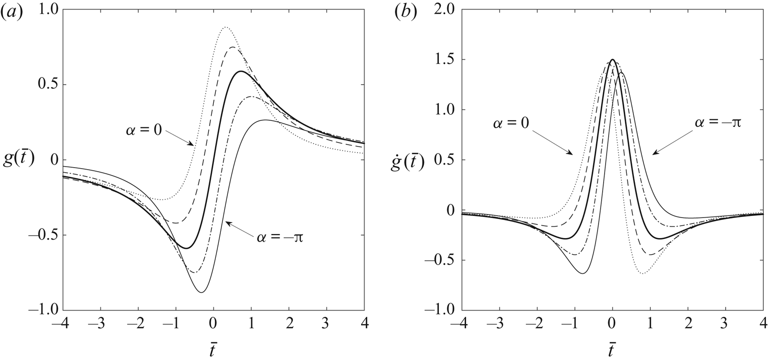
Representative time histories of  $g(\bar {t})$ and
 $\dot {g}(\bar {t})$ are provided in figure 3 for five rectilinear paths of the vortex ring past the porous edge,
 $\alpha = 0,-{\rm \pi} /4,-{\rm \pi} /2,-3{\rm \pi} /4,-{\rm \pi}$. Figure 3(b) together with (3.3) indicates that the acoustic pressure for each path changes rapidly near
 $\bar {t}=0$, where the vortex ring passes closest to the edge. Note in figure 3(b) how the acoustic pressure amplitude is affected weakly in the high-porosity limit by the vortex path angle
 $\alpha$. Also, the acoustic waveform in the high-porosity limit described by
 $\dot {g}(\bar {t})$ is symmetric about
 $\bar {t}=0$ for a vortex ring passing perpendicular to the plane of the edge,
 $\alpha =-{\rm \pi} /2$.
Time histories of (a)  $g(\bar {t})$ and (b)
 $\dot {g}(\bar {t})$, in the limit of high porosity,
 $\mu /k \gg 1$. Results are plotted for vortex path angles
 $\alpha = 0,-{\rm \pi} /4,-{\rm \pi} /2,-3{\rm \pi} /4,-{\rm \pi}$ relative to the porous edge. The heavy line corresponds to
 $-{\rm \pi} /2$.

3.3. General porosity case
The acoustic pressure solution (2.17) for arbitrary values of the dimensionless porosity parameter  $\mu /k$ requires numerical evaluation. We now consider the case of arbitrary porosity effects, where the acoustic pressure is determined strictly by (2.29). The waveform of the acoustic pressure is determined directly by fractional derivative
 $\text {D}_{\bar {t}}^{m}[g(\bar {t})]$, which can be evaluated in the Caputo sense (Podlubny Reference Podlubny1998):
 \begin{align} \text{D}_{\bar{t}}^{m}[g(\bar{t})] &= \frac{1}{2{\rm \pi}}\int_{-\infty}^{+\infty}{(-\mathrm{i}\omega)^{m}\,\hat{g}(\omega)\, \text{e}^{-\mathrm{i}\omega {\bar{t}}}\, {\rm d} \omega}\nonumber\\ &=\frac{1}{\mathcal{G}(1-m)}\int_{-\infty}^t{\frac{\dot{g}(s)}{({\bar{t}}-s)^{m}}\, {\rm d} s}, \end{align}
where the full expression for  $\dot {g}(s)$ is given in Appendix B, and
 $\mathcal {G}$ is the well-known gamma function. The value of parameter
 $m$ for the leading solution term follows (A13) and varies on the dimensionless porosity parameter
 $\mu /k$, and this dependence is plotted in figure 6 in Appendix A.
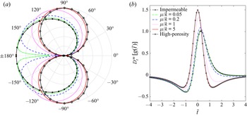
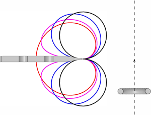
Figure 4 plots the acoustic directivity and the corresponding time-dependent pressure waveforms of the noise emitted by a vortex ring passing near a semi-infinite porous edge, as a function of the dimensionless porosity parameter. Appendix A details the process of evaluation from  $M(\psi, \theta )$, where
 $\psi = {\rm \pi}/2$. The transition of acoustic directivity from a cardioid to a dipole occurs smoothly with increasing values of the porosity parameter. Figure 4(b) illustrates how the asymmetric pressure waveform for impermeable edges found in § 3.1 becomes increasingly symmetric as the porosity parameter increases, where the direction of the vortex ring relative to the porous edge affects the waveform shape.
Acoustic directivity and corresponding pressure waveforms due to a vortex ring passing near a semi-infinite porous edge with various values and limits of the dimensionless porosity parameter  $\mu /k$. The vortex path angle is
 $\alpha = -{\rm \pi} /2$. (a) Acoustic pressure directivity. (b) Far-field pressure waveforms represented by
 $\text {D}_{\bar {t}}^{m}[g(\bar {t})]$ in (3.6).

The dependence of the acoustic power scalings  $\gamma$ and
 $\upsilon$ on
 $\mu /k$, obtained readily from (2.32) and (A13), are illustrated in figure 5. Both exponent values vary monotonically between the formal asymptotic limits of low porosity (
 $\mu /k \ll 1$) and high porosity (
 $\mu /k \gg 1$). Figure 5 indicates that these limits may be refined by numerical computation, where the edge is effectively impermeable for
 $\mu /k < O(10^{-2})$ and the high-porosity limit is achieved for
 $\mu /k > O(10)$.
Dependence of scaling exponents  $\gamma$ and
 $\upsilon$ on dimensionless porosity parameter
 $\mu /k$. Acoustic power is proportional to
 $U^{\gamma }L^{-\upsilon }$.

4. Conclusions
Acoustic emission by a vortex ring near a porous edge is considered analytically and numerically. The mathematical approach integrates and extends the vortex ring acoustic analysis of Kambe et al. (Reference Kambe, Minota and Ikushima1985) for an impermeable edge and the porous edge scattering analysis of Jaworski & Peake (Reference Jaworski and Peake2013) to furnish a time-dependent Green's function for porous edge noise generation. Changes to the time-dependent acoustic pressure and its angular dependence in the acoustic far field depend solely on a single dimensionless porosity parameter  $\mu /k$, and the principal result (2.29) predicts the acoustic power scaling relative to the velocity of vortex ring
 $U$ and the nearest distance of the vortex ring to the edge
 $L$. Special attention is paid to the parametric transition from impermeable to high effective porosity limiting edge conditions, where the gradual change in sound pressure directivity is accompanied by a monotonic change in acoustic power scaling from
 $U^5 L^{-4}$ to
 $U^6 L^{-5}$. These directivity and source speed scaling results for a vortex ring confirm by analogue known results from turbulence noise analysis (Ffowcs Williams & Hall Reference Ffowcs Williams and Hall1970; Jaworski & Peake Reference Jaworski and Peake2013). The complete analysis developed here for porous edges enables the transition from impermeable to porous edge acoustic behaviours to be examined independently in terms of scaling on
 $U$, scaling on
 $L$, and the waveform of the acoustic emission on the dimensionless porosity parameter. The analytical model developed in the present work constitutes the theoretical basis to interrogate the associated experimental campaign presented in Part 2.
Funding
The authors acknowledge the support of the National Science Foundation under awards 1804445 and 1805692.
Declaration of interests
The authors report no conflict of interest.
Appendix A. Green's function for a porous edge
Application of the Fourier inversion formula (2.5) to (2.3) yields
 \begin{equation} (\nabla^2+k^2)\,\hat{G}(\boldsymbol{x},\boldsymbol{y};k) = \delta(\boldsymbol{x}-\boldsymbol{y}), \end{equation}
where  $k=\omega /c$ is the wavenumber and
 $\omega$ is the angular frequency. Here,
 $\boldsymbol {x}=(x_1,x_2,x_3)$ and
 $\boldsymbol {y}=(\kern 0.05em y_1,y_2,y_3)$ represent the positions of the observer and the source, respectively.
By appeal to the reciprocal theorem (Rayleigh Reference Rayleigh1945), the positions of observer and source may be interchanged without modifying the Green's function, i.e.  $\hat {G}(\boldsymbol {x},\boldsymbol {y};k) = \hat {G}(\kern 0.06em\boldsymbol {y},\boldsymbol {x};k)$. Therefore, the Green's function may be expressed as
 \begin{equation} \hat{G}(\boldsymbol{x},\boldsymbol{y};k) = \hat{G}_0(\kern 0.06em \boldsymbol{y},\boldsymbol{x};k) + \hat{G}_s(\kern 0.06em \boldsymbol{y},\boldsymbol{x};k), \end{equation}
where  $\hat {G}_0(\kern 0.06em\boldsymbol {y},\boldsymbol {x};k)$ is the incident spherical wave generated by point source
 $\boldsymbol {x}$ in free space,
 \begin{equation} \hat{G}_0(\kern 0.06em \boldsymbol{y},\boldsymbol{x};k) ={-}\frac{1}{4{\rm \pi}|{\boldsymbol{x}-\boldsymbol{y}}|}\,{\rm e}^{\text{i} k |{\boldsymbol{x}-\boldsymbol{y}}|}, \end{equation}
and  $\hat {G}_s(\boldsymbol {x},\boldsymbol {y};k)$ is the scattered solution due to the interaction of the incident field
 $\hat {G}_0$ and the solid body (edge). At large distances of the source from the edge, where
 $x=|{\boldsymbol {x}}| \rightarrow \infty$,
 $\hat {G}_0$ can be expressed asymptotically as
 \begin{equation} \hat{G}_0(\boldsymbol{x},\boldsymbol{y};k) \sim A \exp [-\text{i}k(\hat{x}_1y_1 + \hat{x}_2y_2)], \end{equation}
where
 \begin{equation} A ={-}\frac{1}{4{\rm \pi} x}\exp (\text{i}kx - \text{i}k\hat{x}_3y_3) \end{equation}
and the direction of the source  $\boldsymbol {x}$ is denoted by
 $$\begin{gather} \hat{\boldsymbol{x}}=\boldsymbol{x}/x= (\hat{x}_1, \hat{x}_2, \hat{x}_3), \end{gather}$$
 $$\begin{gather}\hat{x}_1=\sin{\psi_0}\cos{\theta_0},\quad \hat{x}_2=\sin{\psi_0}\sin{\theta_0},\quad \hat{x}_3=\cos{\psi_0}. \end{gather}$$
From the result of the scattered field for a porous edge by Jaworski & Peake (Reference Jaworski and Peake2013), the corresponding Green's function for the scattered field may be determined:
 \begin{equation} \hat{G}_s(\kern 0.06em \boldsymbol{y},\boldsymbol{x};k) ={-}\frac{1}{2}\text{i} Y^{{1}/{2}} {\rm \pi}^{-{3}/{2}}B\sin{\frac{\theta}{2}}\,\frac{\exp \left[\text{i}kx - \text{i}k\cos{\psi_0}y_3 +\dfrac{\rm \pi}{4}\text{i}\right]}{x}\quad\text{as } Y\rightarrow 0, \end{equation}
where  $Y= (\kern 0.05em y_1^2 +y_2^2)^{{1}/{2}}$ is the projection of
 $\boldsymbol {y}$ on the
 $(\kern 0.05em y_1,y_2)$-plane. Here,
 $B$ is a variable that depends on the wavenumber
 $k$, the properties of the porous edge, and the directivity of the incident field:
 \begin{equation} B = \frac{k\sin{\psi_0}\sin{\theta_0}}{K_{+}(k\sin{\psi_0}\cos{\theta_0})}, \end{equation}
where  $K_{+}(k\sin {\psi _0}\cos {\theta _0})$ is the ‘plus’ function of the associated Wiener–Hopf kernel
 $K(\alpha )$ after multiplicative factorisation, denoted
 $K_{+}(\alpha )$ by Jaworski & Peake (Reference Jaworski and Peake2013, (4.12)).
The kernel function  $K(\alpha )$ can be rewritten as
 $K(\alpha ) = (\alpha + k)^{1/2}(\alpha - k)^{1/2}\,J(\alpha )$, where
 $(\alpha \pm k)^{1/2}$ are regular in the upper/lower half-planes of complex variable
 $\alpha$, and
 $J(\alpha )\rightarrow 1$ as
 $|{\alpha }|\rightarrow \infty$. Therefore,
 \[ K_{+}(\alpha) = (\alpha + k)^{1/2}\,J_{+}(\alpha), \]
where
 \begin{equation} J_{+}(\alpha) = {\rm{exp}}\left[\frac{1}{2{\rm \pi} {\rm{i}}}\int_{\mathcal{C}}\frac{\log J(\xi)}{\xi - \alpha}\, {\rm d} \xi\right]. \end{equation}
The integration contour  $\mathcal {C}$ is chosen and extends from
 $-\infty$ to
 $+\infty$ on the real axis to avoid the branch cuts from
 $\pm k$ to
 $\pm k \pm \rm {i}\infty$. Note that
 $K_{+}(\alpha )$ must be determined numerically, but may be evaluated asymptotically in the limits of low or high edge porosity. At this point the reciprocal theorem is evolved to revert to the original source–observer configuration, which removes the subscripts on the angular positions. The analytical expressions for
 $B$ have been determined by Jaworski & Peake (Reference Jaworski and Peake2013) for two asymptotic limits of low and high effective porosity:
 \begin{align} B \sim \left\{ \begin{array}{ll} (2k)^{1/2}\sin{\dfrac{\theta}{2}}\,(\sin{\psi})^{1/2}, & \mu/k \ll 1,\\[6pt] \mu^{{-}1/2} k\sin{\theta}\sin{\psi}, & \mu/k \gg 1, \end{array} \right. \end{align}
where  $\mu /k=\alpha _H \bar {K}_R/kR$ is the dimensionless porosity parameter.
For the purpose of investigating acoustic pressure directivity and scaling behaviours, it is convenient to express  $B$ as
 \begin{equation} B = M(\psi,\theta)\,k^m \mu^n, \end{equation}
where  $m$ and
 $n$ are the exponents of the wavenumber
 $k$ and the parameter
 $\mu = \alpha _H \bar {K}_R/R$ composed of porosity of the half-plane, respectively, as described in detail in § 2.2. The far-field directivity in this reciprocal problem for the scattered field follows from evaluating
 $M(\psi, \theta )$ for fixed
 $\psi$ and varying
 $\theta$ from
 $-{\rm \pi}$ to
 ${\rm \pi}$. Note that both
 $M(\psi,\theta )$ and
 $m$ vary with the porosity parameter
 $\mu$, and must be determined numerically in general.
Equations (A9) and (A12) permit  $m$ to be computed as
 \begin{equation} m = 1 - {\frac{\partial{\log[K_{+}(k\cos{\theta})]}}{\partial{\log{k}}}}, \end{equation}
for  $\psi = {\rm \pi}/2$ and
 $\mu = 1$. Figure 6 plots the dependence of
 $m$ on
 $\mu /k$ for
 $\theta = {\rm \pi}/4$, whose value does not affect these results.
Dependence of wavenumber parameter  $m$ on the dimensionless porosity parameter
 $\mu /k$.

Appendix B. Expression of  $\dot {g}(s)$

Equations (2.26) and (2.27a,b) yield
 \begin{equation} g(s) = (s^2+1)^{-3/4}\sin\left[\frac{3}{2}\tan^{{-}1}\left(\frac{s\sin{\alpha}\mp \cos{\alpha}}{s\cos{\alpha}\pm\sin{\alpha}}\right)-2\alpha\right]. \end{equation}
The first derivative of  $g(s)$ is obtained by direct application of the chain rule:
 \begin{align} \dot{g}(s)& ={-}\frac{3}{2}s(s^2+1)^{-{7}/{4}}\sin\left[\frac{3}{2}\tan^{{-}1} \left(\frac{s\sin{\alpha}\mp \cos{\alpha}}{s\cos{\alpha}\pm\sin{\alpha}}\right)-2\alpha\right]\nonumber\\ &\quad \pm\frac{3}{2}(s^2+1)^{-{7}/{4}}\cos\left[\frac{3}{2}\tan^{{-}1} \left(\frac{s\sin{\alpha}\mp \cos{\alpha}}{s\cos{\alpha}\pm\sin{\alpha}}\right)-2\alpha\right], \end{align}
where the upper sign holds for  $0 \leq \alpha \leq {\rm \pi}$, and the lower sign holds for
 $-{\rm \pi} \leq \alpha \leq 0$. Note that (B 2) is used for the evaluation of the integral in (3.6) and is equivalent to (3.5).
Appendix C. Estimate of vortex-edge interaction time
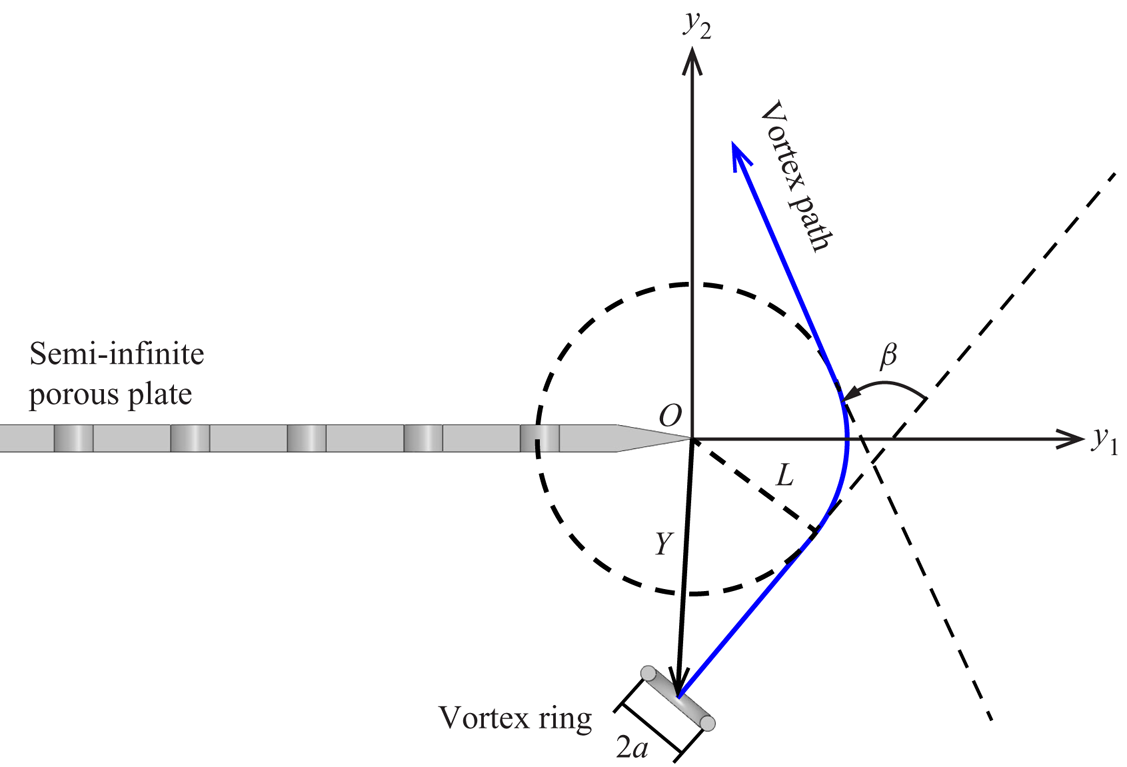
Kambe et al. (Reference Kambe, Minota and Ikushima1985, figure 6) and Yoas (Reference Yoas2021, figure 4.1) indicate experimentally that the path of a vortex ring near a porous edge is not perfectly rectilinear due to its hydrodynamic interaction with the edge, where the change in path becomes more pronounced with increasing vortex ring speed (or circulation, cf. (2.30)). Figure 7 illustrates an idealisation of the modified path, where the vortex ring approaches along a straight path, turns by angle  $\beta$ towards the edge along a circular arc of radius
 $L$, and leaves along a different straight path. The model developed in § 2 for a single rectilinear vortex ring path is justified if the duration of time over which the path turns is small relative to the period of the acoustic waveform.
Schematic of a vortex ring path (blue) affected by hydrodynamic interactions with a semi-infinite porous edge. The vortex path is idealised as three continuous segments: two rectilinear segments and one circular arc with radius  $L$. The turning angle of the vortex path is denoted as
 $\beta$.

Here, it is assumed conservatively that the vortex ring maintains the same speed  $U$ in the circular arc as is does on the rectilinear segments. The dimensionless traverse time of the vortex ring in the arc segment may be estimated as
 \begin{equation} \bar{t}_a = \frac{Ut_a}{a} = \frac{L}{a}\,\beta, \end{equation}
where  $t_a = (L\beta )/U$,
 $\beta$ is the turning angle of the vortex path, and
 $a$ is the radius of the vortex ring. In Yoas (Reference Yoas2021),
 $L = 9.8$ mm and
 $a = 6.5$ mm, and the maximum value of the turning angle
 $\beta$ is approximately
 $13.3^{\circ }$. Furthermore, figure 4(b) suggests a dimensionless acoustic waveform period of approximately 8. Therefore, the ratio of the vortex-edge interaction time and the effective period of the waveform is approximately
 $\bar {t}_a/8 = 4.4\,\%$. Therefore, the influence of the path turning due to the vortex-edge interaction on the entire pressure waveform is marginal and may be neglected in the present work.