1. Introduction
Accurate 3-D models are essential for many applications, such as search and rescue [Reference Zhang, Zhang, Li, Yuan and Fang1], cave surveying [Reference Li, Savkin and Vucetic2, Reference Tabib, Goel, Yao, Boirum and Michael3], and environment perception [Reference Yuan, Huang, Sun and Tao4]. Generally, 3-D models of large structures can be reconstructed by robotic coverage. However, existing robotic coverage methods typically require a prior 3-D model of the target as input and plan the robotic coverage path offline. In contrast, robotic exploration methods do not require any prior knowledge and can explore unknown environments online. Nevertheless, existing exploration planning works usually utilize a volumetric map to describe the environment instead of the reconstructed 3-D surface model.
In this paper, we investigate the informative path planning problem for autonomous online 3-D modeling of unknown structures by using micro aerial vehicles (MAVs) equipped with limited on-board sensors. As mentioned above, robotic coverage methods usually plan the coverage path for fully known or at least partially-known structures [Reference Jing, Deng, Xiao, Liu and Shimada5–Reference Tang and Ma7]. These methods typically incorporate three steps for constructing accurate 3-D models: first, solving the model-based offline coverage path planning problem under a variety of perception constraints; second, performing online data collection during the MAV flight; lastly, converting the recorded data to a 3-D model utilizing off-the-shelf 3-D reconstruction pipelines. It is a tedious and time-consuming procedure and not suitable for time-sensitive applications (e.g. search and rescue missions [Reference Delmerico, Mintchev, Giusti, Gromov, Melo, Horvat, Cadena, Hutter, Ijspeert, Floreano, Gambardella, Siegwart and Scaramuzza8]). Different from robotic coverage, autonomous robotic exploration can model unknown structures online by constructing a volumetric map of the target [Reference Bircher, Kamel, Alexis, Oleynikova and Siegwart9–Reference Yu, Shen, Xu and Zhang14]. However, a complete volumetric map does not imply that the resulting 3-D model is accurate and complete (i.e. it may leave holes on the reconstructed surfaces). To achieve high-quality online 3-D modeling of unknown structures, one should concurrently execute exploration and coverage in a unified planning framework.
We propose the Simultaneous Exploration And Coverage planner (SEAC) for autonomous online 3-D modeling of unknown structures based on informative path planning. First, we devise a set of metrics that take into account the perception constraints of the on-board sensor for evaluating the coverage quality of the reconstructed surfaces. These metrics can be computed quickly during the construction of the Truncated Signed Distance Field (TSDF) model. The evaluation results of the surface coverage quality are then stored in the TSDF model for the subsequent viewpoint utility calculation. Second, SEAC adopts a hierarchical framework consisting of two planning stages to achieve high coverage quality and exploration efficiency simultaneously. At the local coverage stage, the MAV will compute the local coverage path within a local planning horizon. Specifically, the viewpoint with the maximum local exploration utility is first selected as the planning goal. Then, the local coverage path with the highest coverage utility is obtained by solving a submodular orienteering problem. When there are no frontiers and uncovered surfaces in the local planning horizon, the planner will turn to the global exploration stage. At this stage, the MAV can quickly find a safe and efficient global exploration path on a sparse roadmap. The sparse roadmap is incrementally expanded during the MAV flight and the positions of its nodes are continuously updated utilizing the constructed Euclidean signed distance fields (ESDFs). Our method is validated in realistic simulations by comparing it with state-of-the-art methods. The comparative results demonstrate that our method outperforms other methods in terms of both reconstruction accuracy and completeness, without compromising exploration efficiency. Finally, we integrate SEAC into a self-built MAV and validate it through an indoor experiment.
The main contributions of this work are the following:
-
1. We devise a set of efficiently computable metrics for evaluating the coverage quality of the reconstructed surfaces that incorporates perception constraints of the on-board sensor. These evaluation metrics can greatly facilitate the viewpoint utility evaluation that is essential to the performance of SEAC.
-
2. We propose a novel planner that performs simultaneous exploration and coverage (SEAC). Our planner optimally balances between local coverage effort for inspecting low-quality surfaces and global exploration effort for extending the map.
-
3. We benchmark the performance of SEAC through simulation trials, demonstrating its superiority. In addition, the effectiveness of SEAC is also validated by the real-world experiment.
2. Related work
2.1. Path planning for robotic coverage
The objective of coverage path planning (CPP) is to compute the motion path for robots achieving complete coverage of the target with the on-board sensor. Existing algorithms to CPP problem typically require the prior information of the target and compute the coverage path offline. The typical workflow of CPP algorithms consists of three steps, i.e. viewpoints generation, CPP and execution, and offline data processing [Reference Jing, Deng, Xiao, Liu and Shimada5–Reference Tang and Ma7, Reference Sharma and Voruganti15, Reference Wang, Zhang, Zhang, Zhang and Liu16]. Different from most CPP algorithms, Roberts et al. [Reference Roberts, Shah, Dey, Truong, Sinha, Kapoor, Hanrahan and Joshi17] proposed the explore-then-exploit strategy to achieve CPP without any prior knowledge of the target. In the explore phase, the MAV is commanded to execute a default trajectory at a safe distance above the target while acquiring a sequence of images. After that, a coarse 3-D model of the target can be generated by processing the obtained images. In the exploit phase, the 3-D coverage path is computed based on the coarse model to maximize the fidelity of the resulting 3-D model. Although the strategy results in higher-quality 3-D reconstructions, it still can not be directly used in time-sensitive applications.
2.2. Path planning for robotic exploration
Exploration path planning (EPP) algorithms can be roughly classified into sampling-based methods and frontier-based methods [Reference Bircher, Kamel, Alexis, Oleynikova and Siegwart9–Reference Yu, Shen, Xu and Zhang14, Reference Liu, Wang, Chi, Chen and Sun18]. Sampling-based methods usually sample viewpoints or paths based on the rapidly-exploring random tress (RRT) [Reference Chi, Wang, Ding, Chen and Sun19] and select the candidate with the largest exploration utility as the exploration goal [Reference Bircher, Kamel, Alexis, Oleynikova and Siegwart9, Reference Respall, Devitt, Fedorenko and Klimchik10]. In contrast to sampling-based methods, frontier-based methods guide the exploration process by visiting frontiers [Reference Tao, Wu, Li, Cladera, Zhou, Thakur and Kumar11–Reference Yu, Shen, Xu and Zhang14]. Therefore, the important problem for frontier-based methods to solve is the sequence to visit frontiers. Generally, the optimal frontier visiting sequence can be computed by solving the traveling salesman problem (TSP) [Reference Cao, Zhu, Choset and Zhang20]. Up to now, the EPP problem has been widely investigated, and there are many promising algorithms that have been proposed for mapping unknown environments online. Nevertheless, EPP algorithms only focus on observing unexplored space, and the reconstruction quality of the target structure is not explicitly considered, which usually results in poor reconstruction quality or even leaves holes on the obtained 3-D model.
2.3. Path planning for simultaneous exploration and coverage
Recently, the path planning problem for online 3-D modeling of unknown structures has been investigated [Reference Heng, Gotovos, Krause and Pollefeys21–Reference Schmid, Pantic, Khanna, Ott, Siegwart and Nieto26]. Heng et al. [Reference Heng, Gotovos, Krause and Pollefeys21] first proposed the strategy that can simultaneously explore and cover unknown environments. However, their strategy requires indispensable pre-computation operations before the online planning. The work in [Reference Vutetakis and Xiao22] proposed to utilize surface frontiers to extend the model of the target structure. Sungho et al. [Reference Song and Jo23] proposed a novel hierarchical online 3-D modeling planner. This planner first computes the sector visitation order and then plans the local inspection path to enhance the accuracy of the resulting 3-D model. However, in their work, the confidence of surfaces is estimated through Poisson surface reconstruction, which requires high computational cost. Similarly, Feng et al. [Reference Feng, Li, Gao, Zhou and Shen24] proposed a seminal hierarchical planner for online aerial 3-D modeling. One limitation of the planner is that it requires pre-training of the surface prediction module, which is utilized to guide the subsequent surface coverage. By contrast, Schmid et al. [Reference Schmid, Pantic, Khanna, Ott, Siegwart and Nieto26] proposed an online informative path planner for 3-D modeling by continuously expanding a single tree. Their planner employs surface frontiers and weights stored in TSDFs to guide the evaluation of coverage viewpoints. However, it does not take into account the perception constraints of the on-board sensor. Furthermore, maintaining a single tree in the explored environment often requires significant computational costs. Most recently, Zhang et al. [Reference Zhang, Feng, Li, Zheng, Luo, Wang, Zhou, Shen and Zhou27] proposed a promising simultaneous exploration and photographing algorithm for fast autonomous 3-D reconstruction of unknown structures using multiple heterogeneous MAVs.
In summary, robotic coverage excels in achieving high-quality 3-D reconstructions of known structures, whereas robotic exploration is suited for constructing models of unknown structures. It is intuitive to achieve high-quality online 3-D modeling of unknown structures by integrating these two techniques within a unified framework. However, existing methods struggle to balance computational efficiency with modeling quality. Therefore, we propose a computationally efficient simultaneous exploration and coverage planner for autonomous online 3-D modeling of unknown structures using an MAV.
3. Problem formulation
3.1. MAV and sensor models
In this work, we consider the robot to be a quadrotor-type MAV equipped with a forward-looking depth sensor, and we assume the MAV can localize itself perfectly.
MAV Model: We follow the idea proposed in ref. [Reference Faessler, Franchi and Scaramuzza28] to exploit the differential flatness of MAVs, that is, only four selected flat outputs are considered as follows
 \begin{equation} {\textrm {x}} \,:\!=\, \{\textbf {p}, \psi \} \in \mathcal{X} \subset \mathbb{R}^4, \end{equation}
where
 $\bf{p} =$
 $[x,y,z]^T \in \mathbb{R}^3$
is the position of the MAV and
 $\psi$
 $\in$
 $[-\pi ,\pi )$
is the yaw angle at that position. At a state (also called viewpoint)
 $\textrm {x}$
, the MAV collects depth measurements from the sensor and integrates them into the map.
Sensor Model: In order to model the sensor accurately, we adopt the view frustum model that is usually used in the field of robotic coverage [Reference Jiang, Zhang, Chen and Fang29]. We assume that the sensor has its inherent and/or user-defined perception constraints such as a limited field of view (FoV), e.g., it has a truncated perception range,
 $[d_{min},d_{max}]$
,
 $d \in \mathbb{R}^+$
, and horizontal and vertical view angles,
 $\alpha _{h}$
 $\in {(}0,360^\circ {]}$
,
 $\alpha _{v}$
 $\in {(}0,360^\circ {]}$
, respectively.
3.2. Map representation
Generally, for the exploration problem, the volumetric map is a popular map type for the representation of unknown environments. On the other hand, the spline surface [Reference Wang, Zhang, Zhang, Zhang and Liu16] or polygon mesh [Reference Jiang, Zhang, Chen and Fang29] is usually adopted to model the target by robotic coverage works. However, all these representations are not suitable for online 3-D modeling.
In this paper, we decide to utilize an efficient surface reconstruction method, Voxblox [Reference Oleynikova, Taylor, Fehr, Siegwart and Nieto30], for online 3-D modeling. Voxblox is an open-source library that builds TSDFs of the target incrementally and computes the corresponding ESDFs directly from the obtained TSDFs. While Voxblox is also a volumetric-type mapping method, it can generate human-readable surfaces with sub-voxel resolution. To cope with our problem features, Voxblox is modified as follows: first, it computes a high-resolution TSDF model for accurate 3-D modeling as well as the coverage quality of each reconstructed surface for the subsequent viewpoint evaluation using the proposed evaluation metrics; second, it also maintains the ESDFs from a low-resolution TSDF model for efficient collision checking and roadmap maintenance.
3.3. Problem description
In this work, we consider a path planning problem for exploring an unknown but spatially bounded 3-D space
 $\mathcal{V} \subset \mathbb{R}^3$
and simultaneously covering the surfaces
 $\mathcal{S}$
of a structure contained in this space (i.e.
 $\mathcal{S} \subset \mathcal{V}$
). We can obtain a volumetric representation
 $\mathcal{M}$
and a surface model
 $\mathcal{S}$
from the TSDFs of the target space. The volumetric representation
 $\mathcal{M}$
can divide
 $\mathcal{V}$
into tree types: occupied
 $\mathcal{M}_{occ}$
, free
 $\mathcal{M}_{free}$
and unknown
 $\mathcal{M}_{un}$
, thus we have
 $\mathcal{M}_{un}$
 $=$
 $\mathcal{M}$
 $\backslash$
 $\left \{\mathcal{M}_{occ} \cup \mathcal{M}_{free} \right \}$
. The surfaces perceived by the on-board sensor at a viewpoint
 $\textrm {x}$
under the perception constraints will be labeled as covered
 $\mathcal{S}_{cov}$
and the remaining surfaces belonging to uncovered
 $\mathcal{S}_{un}$
. Similar to
 $\mathcal{M}$
, we have
 $\mathcal{S}_{un}$
 $=$
 $\mathcal{S}$
 $\backslash$
 $\mathcal{S}_{cov}$
. Our objective is to simultaneously reduce the voxels belonging to
 $\mathcal{M}_{un}$
and surfaces belonging to
 $\mathcal{S}_{un}$
as much as possible and thus obtain a complete and accurate 3-D model of the target. The problem can be formulated as follows.
Problem 1: Given
 $\mathcal{M}_{un}$
,
 $\mathcal{S}_{un}$
, and the current state of the MAV
 $\textrm {x}_{cur}$
, we compute the optimal path
 $\text{X}^*$
consisting of a sequence of viewpoints
 ${\textrm {x}}_i$
 $(i=1,2,\ldots )$
. The path
 $\text{X}^*$
can be further optimized to be a feasible trajectory
 $\text{X}^*(t)$
using the off-the-shelf algorithms. After that, the MAV will follow
 $\text{X}^*(t)$
and thus observe
 $\mathcal{M}_{un}$
and cover
 $\mathcal{S}_{un}$
. To achieve the objective more efficiently, we want to maximize the utility function when computing the MAV path in each planning epoch as follows
 \begin{eqnarray} {\max \; {\mathcal U}_e({\mathcal L}(\text{X})},\;{\mathcal I}_e({\text{X}})) + {\mathcal U}_c({\mathcal L}(\text{X}),\;{\mathcal I}_c({\text{X}}))\notag\\ {s.t. \left \{ {\begin{array}{*{20}{c}} {\text{X} \subset {{\mathcal M}_{free}}},\;\;\;\;\;\;\;\;\;\;\;\;\;\;\;\;\;\;\;\;\;\;\;\;\;\;\;\;\;\;\;\\ {{\mathcal L}(\text{X} ) \le L_B},\;\;\;\;\;\;\;\;\;\;\;\;\;\;\;\;\;\;\;\;\;\;\;\;\;\;\;\;\;\;\;\\ {g(\text{X} ) \ge 0},\;\;\;\;\;\;\;\;\;\;\;\;\;\;\;\;\;\;\;\;\;\;\;\;\;\;\;\;\;\;\;\;\; \end{array}} \right .} \end{eqnarray}
where
 $\mathcal{L}(\text{X})$
is the motion cost for the robot following the path,
 $\text{X}$
,
 $\mathcal{I}_e({\text{X}})$
and
 $\mathcal{I}_c({\text{X}})$
are the expected exploration gain and coverage information gain that the MAV can obtain along with the path,
 $L_B$
denotes the motion cost budget (e.g. maximum path length or maximum flight time), and
 $g(\text{X}) \ge 0$
denotes that the planned path should meet designated constraints ( e.g. maximum linear velocity and maximum yaw rate ). We can learn that
 ${\mathcal U}_e(\cdot )$
takes as input parameters the motion cost
 $\mathcal{L}(\text{X})$
and the expected exploration gain
 $\mathcal{I}_e(\text{X})$
and returns an evaluation result.
 ${\mathcal U}_c(\cdot )$
takes as input parameters the motion cost
 $\mathcal{L}(\text{X})$
and the expected coverage gain
 $\mathcal{I}_c(\text{X})$
and also returns an evaluation result. The path that maximizes
 ${\mathcal U}_e({\mathcal L}(\text{X}),\;{\mathcal I}_e({\text{X}})) + {\mathcal U}_c({\mathcal L}(\text{X}),\;{\mathcal I}_c({\text{X}}))$
will be selected to explore and cover the environment simultaneously.
4. Methodology
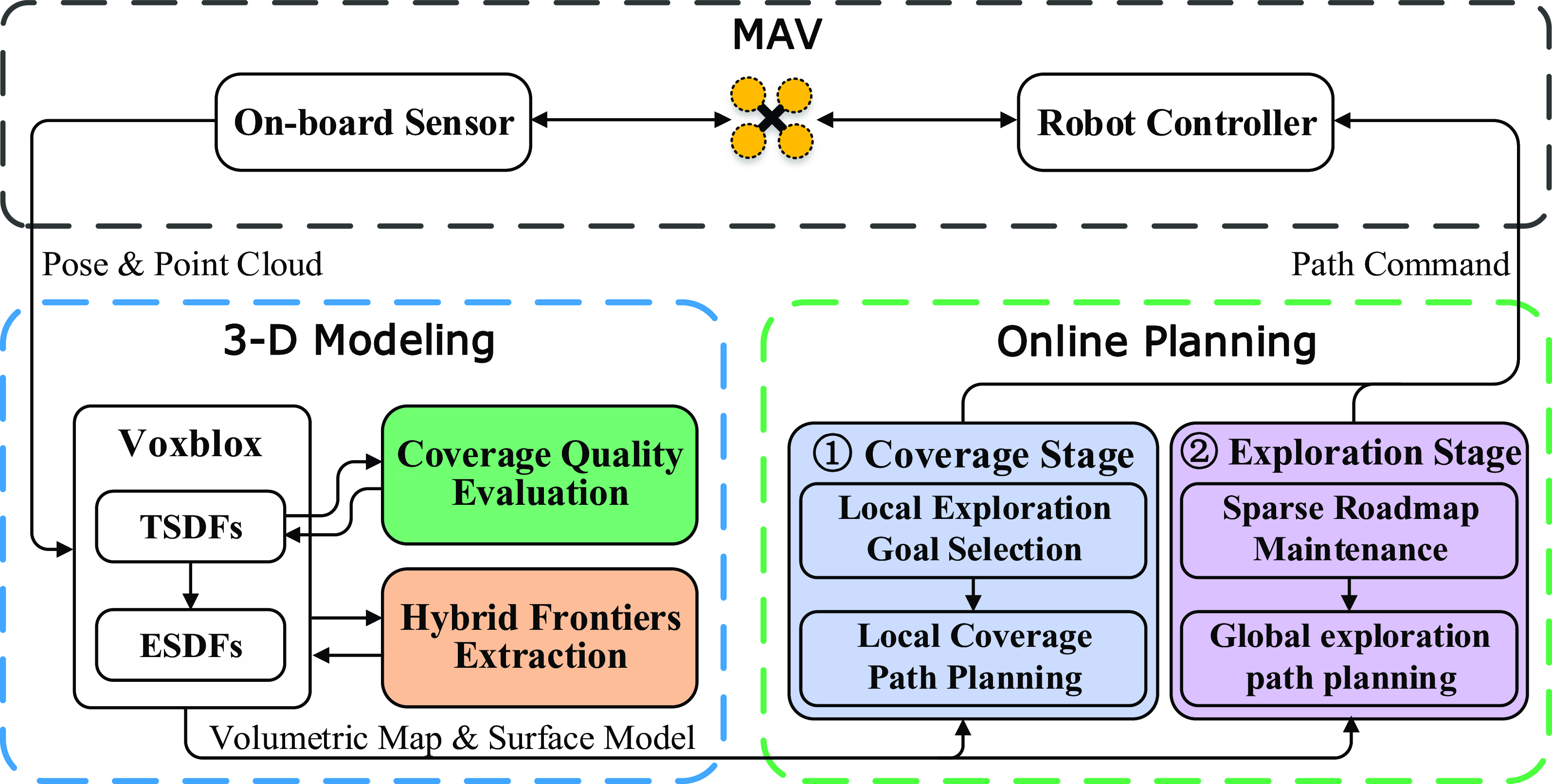
The system overview of SEAC is shown in Figure 1. SEAC has two main components: a 3-D modeling module and a path planning module. The 3-D modeling module integrates the estimated pose and collected depth measurements into Voxblox for volumetric mapping and surface modeling. In addition, whenever the 3-D modeling module is invoked, the coverage quality of each reconstructed surface (Sec. 4.1) as well as hybrid frontiers will be also computed at the same time for facilitating the subsequent path planing (Sec. 4.2). After that, the hierarchical path planning module works to find the optimal path for simultaneously covering uncovered surfaces and exploring unknown space (Sec. 4.3 and Sec. 4.4). Finally, we utilize the SE(3) controller [Reference Lee, Leok and McClamroch31], which takes the current MAV pose and the optimal path provided by the online planner as input, to command the MAV to complete the task. The online 3-D modeling will be terminated when there are no uncovered surfaces and frontiers.
Overview of our simultaneous exploration and coverage planning framework for online 3-D modeling.

4.1. Surface coverage quality evaluation
The TSDF model consists of a set of voxels
 $v$
with a user-defined voxel size
 $r \in \mathbb{R}^+$
. We define the occupied voxel
 $v_s$
containing a reconstructed surface
 $s \in \mathcal S$
as surface voxel. To achieve the best coverage quality, the on-board sensor should observe the target as perpendicularly as possible to its surfaces. Thus, the viewing angle between the ray from the on-board sensor center through the center of
 $v_s$
and the normal to the reconstructed surface
 $s$
should be less than a threshold
 $\theta _{\max }$
. However, the surface normal is difficult to compute directly from the volumetric map. Existing methods usually compute the surface normal by reconstructing the whole surface of the target to obtain the surface normals [Reference Song and Jo23] or fitting a plane around the surface voxel
 $v_s$
[Reference Jung, Song, Youn and Myung32]. Although the above methods can obtain accurate surface normals, the computational complexity is too high, making it intractable to evaluate the surface coverage quality online. Therefore, we present a method to calculate the approximate surface normal and also a set of coverage quality metrics.
Given a reconstructed surface
 $s \in \mathcal S$
, its normal
 ${\textbf {n}}_{{v_s}}$
can be approximately computed from the TSDF model as the distance gradient
 $\nabla {d_s}\left ( v_s \right )$
of
 $v_s$
as follows
 \begin{equation} {\textbf {n}}_{{v_s}} = \sum \limits _{{v_{nbr}} \in N^k_{v_s}} {{d_s}\left ( {{v_{nbr}}} \right ) \cdot \frac {{{\textbf {p}}_{v_{nbr}} - {\textbf {p}}_{v_s}}}{{\left \| {{\textbf {p}}_{v_{nbr}} - {\textbf {p}}_{v_s}} \right \|}}}, \end{equation}
where
 $v_{nbr} \in {N^k_{{{v_s}}}}$
denotes the
 $k$
-connected neighboring voxels of
 $v_s$
,
 ${d_s}(v_{nbr})$
indicates the signed distance of
 $v_{nbr}$
to its nearest surface, and
 ${\textbf {p}}_{v_{nbr}}$
and
 ${\textbf {p}}_{v_s}$
are the positions of
 $v_{nbr}$
and
 $v_s$
, respectively.
Let the index of
 $v_s$
of the TSDF model be
 $(x_s,y_s,z_s)$
, we have
 ${d_s}(v_s)={d_s}(x_s,y_s,z_s)$
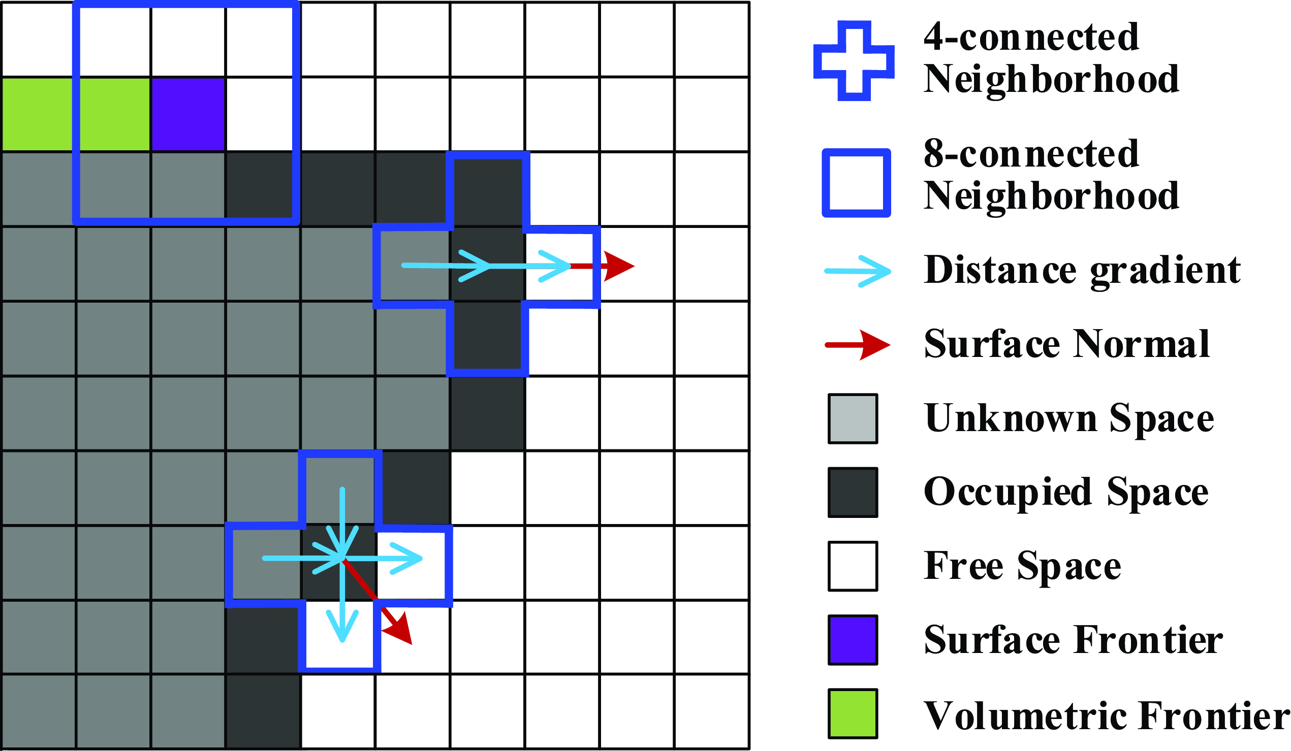
. As shown in Figure 2, when
 $k=6$
, the Eq. (3) can be written as
 \begin{equation} {{\textbf {n}}_{{v_s}}} = \left [ {\begin{array}{*{20}{c}} {{d_s}\left ( {{x_s} + 1,{y_s},{z_s}} \right ) - {d_s}\left ( {{x_s} - 1,{y_s},{z_s}} \right )}\\ {{d_s}\left ( {{x_s},{y_s} + 1,{z_s}} \right ) - {d_s}\left ( {{x_s},{y_s} - 1,{z_s}} \right )}\\ {{d_s}\left ( {{x_s},{y_s},{z_s} + 1} \right ) - {d_s}\left ( {{x_s},{y_s},{z_s} - 1} \right )} \end{array}} \right ], \end{equation}
similarly, we can quickly compute the normal to each reconstructed surface when
 $k=18$
or
 $k=26$
.
Simplified 2-D examples of the surface normal calculation and frontier extraction. The 4/8-connected neighborhood in the 2-D case is a simplification of the 6/26-connected neighborhood in the 3-D case.

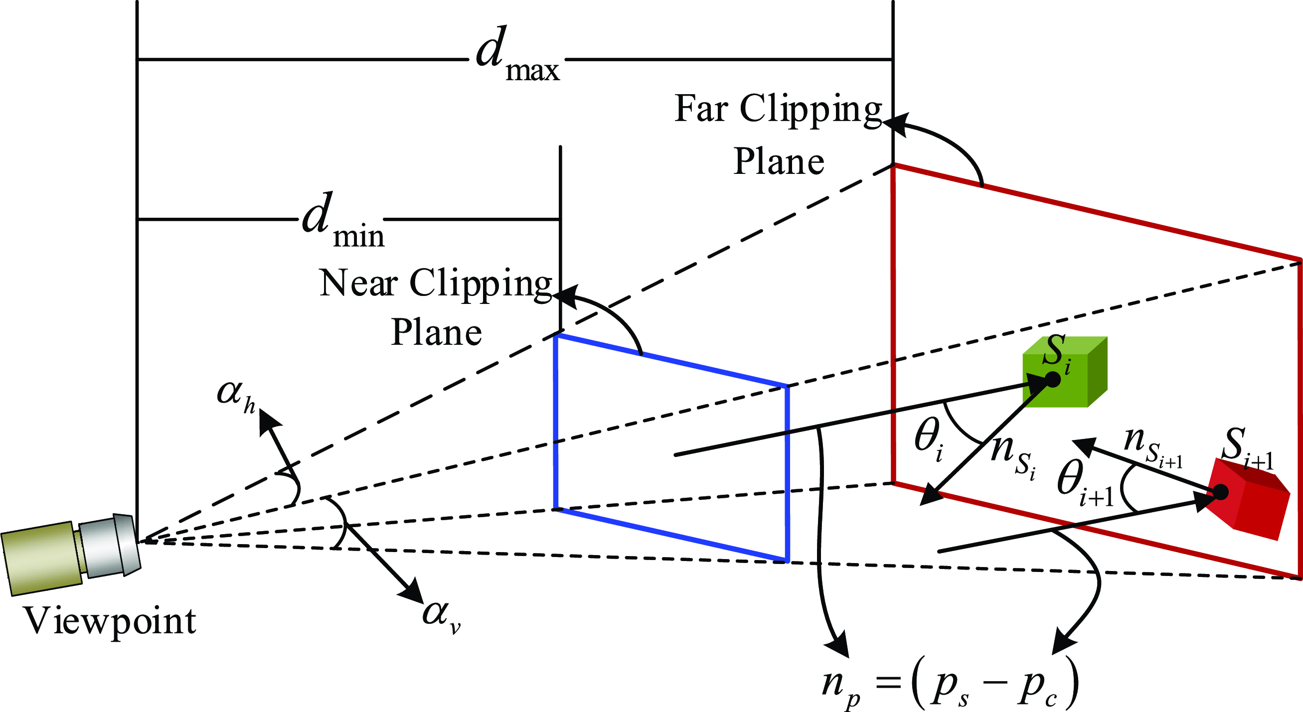
To improve the coverage quality of reconstructed surfaces and thereby effectively reduce the reconstruction error of the target, we adopt the frustum sensor model (see Figure 3) to achieve accurate evaluation of the surface coverage quality. Based on the frustum sensor model and the extracted surface normals, we propose our evaluation metrics that incorporate the perception constraints of the sensor when evaluating the coverage quality of reconstructed surfaces. Specifically, if a surface
 $s_i \in \mathcal S$
is effectively covered by the sensor (indicating it has a high coverage quality), we mark
 $s_i$
as covered, otherwise
 $s_i$
will be marked as uncovered.
Diagram of the frustum sensor model and its perception constraints. It illustrates the relationship between one viewpoint and the normals of surfaces.

4.1.1. Observing angle
 \begin{equation} \left | {\cos ^{ - 1}} \frac {{ {{\textbf {n}}_{s_i}} \cdot \left ( {{{\textbf {p}}_{s_i}} - {{\textbf {p}}_c}} \right )}}{{\left \| {{\textbf {n}}_{s_i}} \right \|\left \| { {{{\textbf {p}}_{s_i}} - {{\textbf {p}}_c}} } \right \|}} \right | \le {\theta _{\max }}, \end{equation}
where
 ${\textbf {n}}_{s_i}$
is the normal to surface
 $s_i$
and
 $\theta _{\max }$
is the designated threshold of the observing angle. This metric is used to determine whether the ray from sensor center to the surface
 $s_i$
is cast appropriately.
4.1.2. Observing distance
 \begin{equation} {d_{\min }} \le \left \| {{{{\textbf {p}}_{s_i}} - {{\textbf {p}}_c}}} \right \| \le {d_{\max }}, \end{equation}
where
 ${\textbf {p}}_{s_i}$
denotes the position of
 $v_{s_i}$
and
 ${\textbf {p}}_c$
is the position of the on-board sensor’s center. The observing distance metric is used to judge whether the reconstructed surface has been observed with a proper distance.
4.1.3. Surface completeness
 \begin{equation} N^{18}_{v_{s_i}} \ge l,\;l \in {{\mathbb{N}}^ + }, \end{equation}
where
 $N^{18}_{v_{s_i}}$
denotes the number of neighboring surfaces of
 $v_{s_i}$
in its 18-connected neighborhood, and the number of neighboring surfaces of
 $v_{s_i}$
should be not less than
 $l$
. The surface completeness metric is used to mitigate the effects of isolated surfaces induced by sensor noise, thereby enhancing the completeness of the reconstructed mesh surface.
When new depth measurements arrives, we first update the TSDF model and compute the normals of newly reconstructed surfaces, and then sequentially determine whether a newly reconstructed surface
 $s$
meets the above metrics. If
 $s$
does not satisfy all the metrics, it will be considered to have low coverage quality ( i.e.
 $s$
will be marked as uncovered) and thus will be carefully inspected later. If
 $s$
satisfies all the evaluation metrics, it will be considered to have high coverage quality ( i.e.
 $s$
will be marked as covered) and will not contribute to the coverage utility evaluation of candidate viewpoints in the subsequent planning iteration.
4.2. Hybrid frontiers extraction
In order to efficiently achieve simultaneous coverage and exploration, we extract two types of frontiers, i.e., the volumetric frontier and the surface frontier.
4.2.1.
Volumetric frontier
 ${\textrm {F}}_v$

A set of connecting free voxels
 $v_{mf} \in \mathcal{M}_{free}$
adjacent to at least one unknown voxel, i.e.,
 ${\textrm {F}}_v = \{v_{mf} \in \mathcal{M}_{free} \,:\, \exists \; neighbor(v_{mf}) \in \mathcal{M}_{un}\}$
.
4.2.2.
Surface frontier
$\textrm {F}_s$

A set of connecting free voxels
 $v_{sf} \in \mathcal{M}_{free}$
adjacent to at least one unknown voxel and at least one occupied voxel, i.e.,
 \begin{eqnarray} \left \{ {\begin{array}{*{20}{c}} {\exists v_u \in N^{8}_{v_{sf}}\;}&{s.t.\;\; \omega \left ( {v_u} \right ) \lt W_{th}, \;\;\;\;\;\;\;\;\;\;\;\;\;\;\;\;\;\;}\\[5pt] {\exists v_o \in N^{26}_{v_{sf}}}&{\;\;s.t.\;\; \omega \left ( {v_o} \right ) \ge W_{th} \wedge d_s\left ( {v_o} \right ) \le 0}, \end{array}} \right . \end{eqnarray}
where
 $v_u$
is an unknown voxel,
 $v_o$
is an occupied voxel,
 $N^{8}_{v_{sf}}$
denotes the 8-connected neighborhood of
 $v_{sf}$
, and
 $N^{26}_{v_{sf}}$
denotes the 26-connected neighborhood of
 $v_{sf}$
.
 $\omega$
is a weight that representing the confidence for the signed distance stored in that voxel, and
 $W_{th}$
is the weight threshold to determine whether a voxel is unknown or not.
In this work, we utilize the frontier detection method proposed in ref. [Reference Zhou, Zhang, Chen and Shen13] to extract frontiers.
 ${\textrm {F}}_v$
and
 $\textrm {F}_s$
will be used to compute the exploration gain and the coverage gain of every viewpoint, respectively.
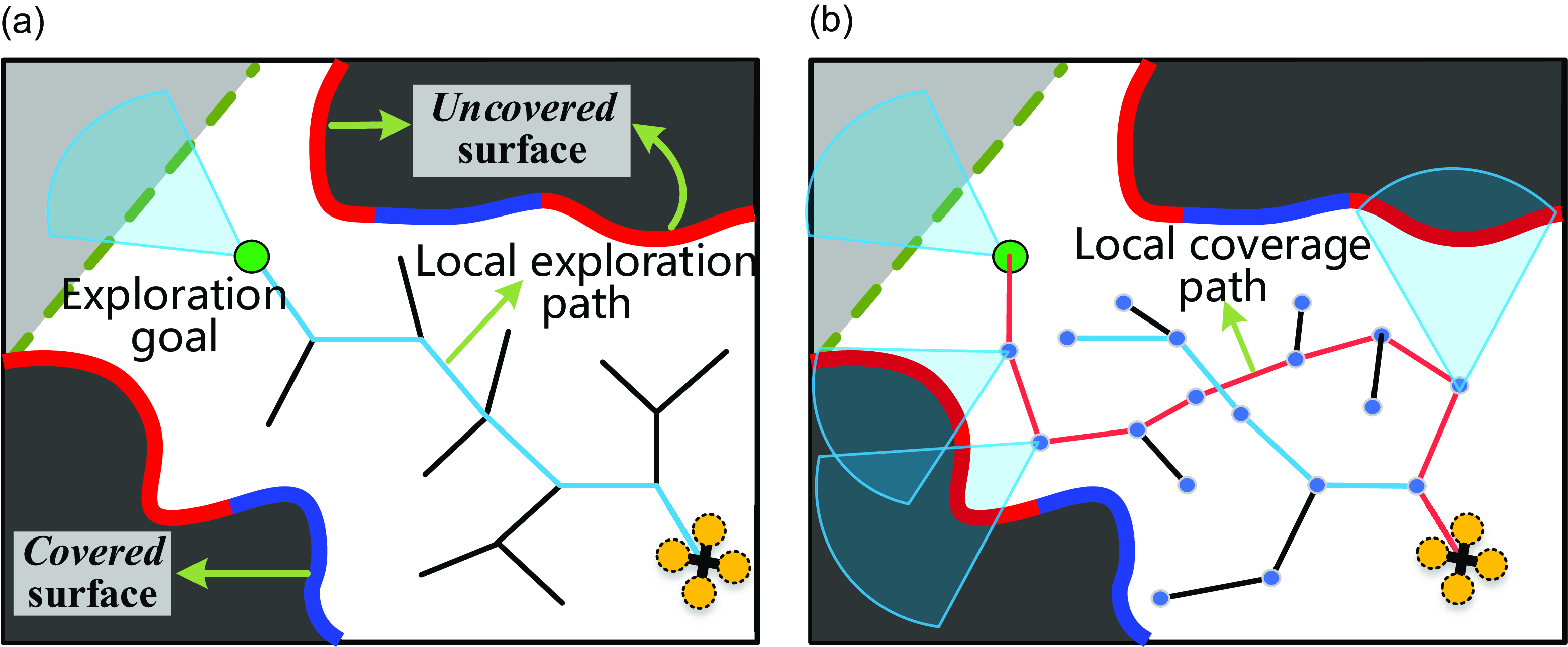
Local coverage stage. (a) The MAV finds the optimal local exploration goal as well as the corresponding local exploration path, which will serve as the initial solution of the local coverage planning problem. (b) The MAV obtains the local coverage pah by solving the submodular orienteering problem.

4.3. Local coverage stage
This planning stage is to generate the local coverage path for the MAV inspecting the uncovered surfaces and extending the map boundary simultaneously. As shown in Figure 4, the planning objective can be achieved by sequentially executing two operations: local exploration goal selection and local CPP, in a local planning horizon
 $\mathcal H$
.
4.3.1. Local exploration goal selection
To find the optimal local exploration goal, our method expands an RRT tree
 $\mathbb T$
by sampling
 ${\mathcal N}_{exp}$
nodes in
 $\mathcal H$
. Meanwhile, the exploration utility of every tree node is evaluated and the node with the largest exploration utility is selected as the local exploration goal
 ${\textrm {x}}_{l}^*$
. The expected exploration utility of one tree node can be calculated similarly to [Reference Bircher, Kamel, Alexis, Oleynikova and Siegwart9] as follows
 \begin{equation} {{\mathcal U}_e}({\textrm {x}}_i) = {\mathcal I}_e\left ({{\textrm {x}}_i} \right ){e^{ - \lambda _1 {\mathcal L} \left ( \gamma _e ({\textrm {x}}_{r}, {\textrm {x}}_{i}) \right )}}, \end{equation}
where
 ${\textrm {x}}_{i}$
is a node on the tree
 $\mathbb T$
( i.e., the exploration viewpoint),
 ${\mathcal I}_e({\textrm {x}}_{i})$
is the exploration gain of
 ${\textrm {x}}_{i}$
,
 ${\mathcal L}\left ( \gamma _e ({\textrm {x}}_{r}, {\textrm {x}}_{i}) \right )$
denotes the motion cost,
 $\lambda _1$
is a tunable parameter to penalize the motion cost.
 ${\mathcal I}_e({\textrm {x}}_{i})$
can be calculated by
 \begin{equation} {{\mathcal I}_{e}({\textrm {x}}_i)} = \sum \limits _{v \in Vis({\textrm {x}}_i)} {\left \{ {\begin{array}{*{20}{c}} {1,}&{v \in {\mathcal{M}_{un}},}\\ {1,}&{v \in {{\textrm {F}}_v},}\\ {0,}&{\mbox{otherwise},} \end{array}} \right .} \end{equation}
where
 $Vis({\textrm {x}}_i)$
denotes the collection of all visible voxels that can be observed at the exploration viewpoint
 ${\textrm {x}}_{i}$
. We can learn that
 ${\mathcal I}_e({\textrm {x}}_{i})$
is the total number of unknown voxels and volumetric frontier voxels that can be observed at
 ${\textrm {x}}_{i}$
.
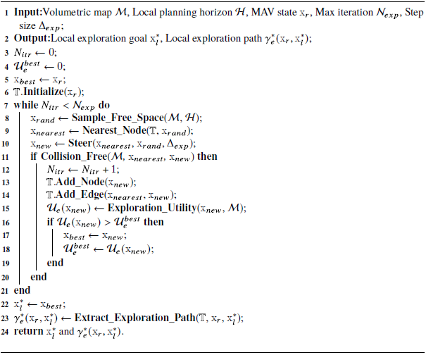
The workflow of the local exploration goal selection is presented in Alg. 1. First, the exploration tree
 $\mathbb T$
is initialized (Alg. 1, lines 3–6). After that,
 ${\mathcal N}_{exp}$
feasible nodes will be sampled in the free space of
 $\mathcal H$
to expand
 $\mathbb T$
(Alg. 1, lines 7–21), meanwhile, the exploration utility
 ${{\mathcal U}_e}({\textrm {x}})$
of each sampled node is computed by the function Exploration_Utility(), according to Eq. (9) and Eq. (10) (Alg. 1, line 15). When the tree expansion is finished, the node with the largest exploration utility will be selected as the local exploration goal
 ${\textrm {x}}_{l}^*$
, and the corresponding local exploration path
 $\gamma _e^* ({\textrm {x}}_{r}, {\textrm {x}}_{l}^*)$
can be recursively extracted from
 ${\textrm {x}}_{l}^*$
to
 ${\textrm {x}}_{r}$
on the tree
 $\mathbb T$
by the function Extract_Exploration_Path() (Alg. 1, lines 22-24, see Figure 4(a)).
Local exploration goal selection

4.3.2. Local coverage path planing
With the local exploration goal in hand, the local coverage path
 $\gamma _c\left ({\textrm {x}}_r, {\textrm {x}}_l^* \right )$
can be obtained by solving a maximization problem. Specifically, the CPP problem is described as follows
 \begin{align}& \gamma _c^* = {\mathop {\arg \max }\limits _{{\gamma _c}\; \subset \;{\mathcal H}}}\;\;{{{\mathcal U}_c}\left ( \gamma _c ({\textrm {x}}_r, {\textrm {x}}_l^*) \right )} \end{align}
 \begin{align}&\qquad {s.t. \left \{ {\begin{array}{*{20}{c}} {\gamma _c \subset {{\mathcal M}_{free}}},\\ {{\mathcal L}(\gamma _c ) \le L_B}, \end{array}} \right .} \end{align}
where
 ${\mathcal L}(\gamma _c ) \le L_B$
denotes that the motion cost budget ( i.e., the path length) should be considered when the MAV achieves the optimal coverage,
 ${{\mathcal U}_c} \left ( \gamma _c ({\textrm {x}}_r, {\textrm {x}}_l^*) \right )$
is the coverage utility that can be obtained along the coverage path. If the coverage gain of the viewpoint is modular, then the above maximization problem is a standard orienteering problem [Reference Vansteenwegen, Souffriau and Oudheusden33]. However, the coverage gain is submodular since the viewpoints might have overlapping FoVs, that is, one surface
 $s$
can be observed by multiple viewpoints. Therefore, the above problem is a submodular orienteering problem.
Local coverage path planning

Due to the coverage gain exhibits submodularity, we compute it at one viewpoint
 ${\textrm {x}}_i$
by
 \begin{equation} {{\mathcal I}_{c}({\textrm {x}}_i)} = \sum \limits _{v \in Vis({{\textrm {x}}_i}),\atop v \notin Vis({\textrm {X}_{\textrm {pre}}})} { \left \{{\begin{array}{*{20}{c}} {1,}&{{s} \in {S_{un{\mathop {\textrm cov}}}},}\\ {1,}&{{v} \in {\textrm {F}_{\textrm {s}},}}\\ {0,}&{\textrm {otherwise},} \end{array}} \right .} \end{equation}
where
 ${\textrm {X}}_{pre}$
is the set of previous viewpoints and we have
 ${\textrm {x}}_i \notin {\textrm {X}}_{pre}$
,
 $Vis({\textrm {x}}_i)$
represents the set of voxels can be observed at
 ${\textrm {x}}_i$
. We can learn that
 ${\mathcal I}_c({{\textrm {x}}_i})$
is the total number of uncovered surfaces and surface frontier voxels that have not been covered by any viewpoint in
 ${\textrm {X}}_{pre}$
but can be covered at
 ${\textrm {x}}_{i}$
.
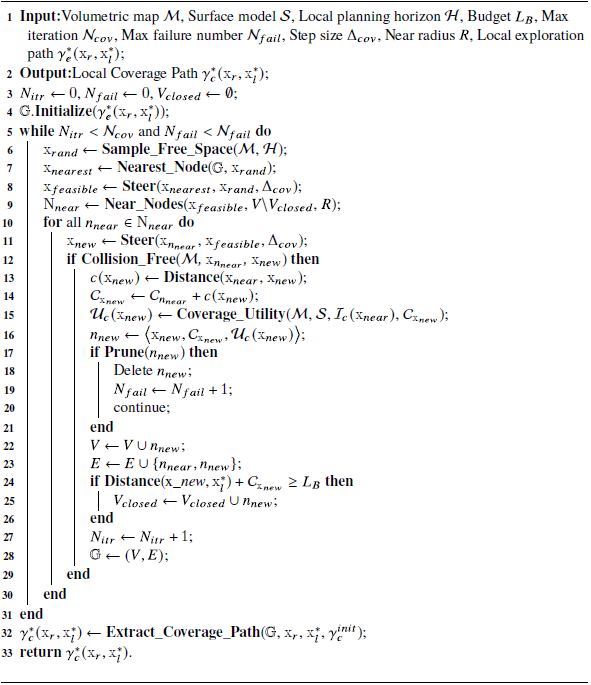
To generate the local coverage path efficiently, we modify the rapidly exploring information gathering (RIG) algorithm [Reference Hollinger and Sukhatme34] for solving Eq. (11). RIG is an informative path planning method that combines sampling-based motion planning with branch and bound algorithms to achieve efficient information gathering under motion constraints. The modified RIG for local CPP is presented in Alg. 2. We set the motion cost budget as
 $L_B = \lambda _2 {\mathcal L} (\gamma _e^* ({\textrm {x}}_{r}, {\textrm {x}}_{l}^*))$
, wherein
 $\lambda _2$
is used to balance the optimality of the resulting path and the real-time performance. When the local exploration path
 $\gamma _e^* ({\textrm {x}}_{r}, {\textrm {x}}_{l}^*)$
is obtained, the algorithm first initializes a graph
 $\mathbb G = \{V,E\}$
using
 $\gamma _e^* ({\textrm {x}}_{r}, {\textrm {x}}_{l}^*)$
(Alg. 2, lines 3–4). After that,
 ${\mathcal N}_{cov}$
feasible nodes will be sampled for expanding the graph. Each time a random state
 ${\textrm {x}}_{rand}$
is sampled, not only the nearest node on the graph will be extended toward
 ${\textrm {x}}_{rand}$
but also all near nodes are trying to extend towards
 ${\textrm {x}}_{rand}$
(Alg. 2, lines 6–9). Meanwhile, their submodular coverage utilities are recursively calculated along all the newly added edges by the function Coverage_Utility(), according to Eqs. (11)–(13) (Alg. 2, line 16). We also prune nodes that are not promising, e.g., those with negligible coverage utility, using the function Prune() (Alg. 2, lines 17–21). In addition, if the expected motion cost (Distance(x_new
 $, {\textrm {x}}_{l}^*$
)
 $+$
 ${\mathcal C}_{{\textrm {x}}_{new}}$
) of the newly extended node exceeds the budget
 $L_B$
, it will be added to the closed set
 $V_{closed}$
and will not be extended in the subsequent process to avoid invalid paths (Alg. 2, lines 24–26). Finally, the local coverage path with the largest coverage utility is recursively extracted from
 ${\textrm {x}}_{l}^*$
to
 ${\textrm {x}}_{r}$
on the graph
 $\mathbb G$
by the function Extract_Coverage_Path() (Alg. 2, line 32).
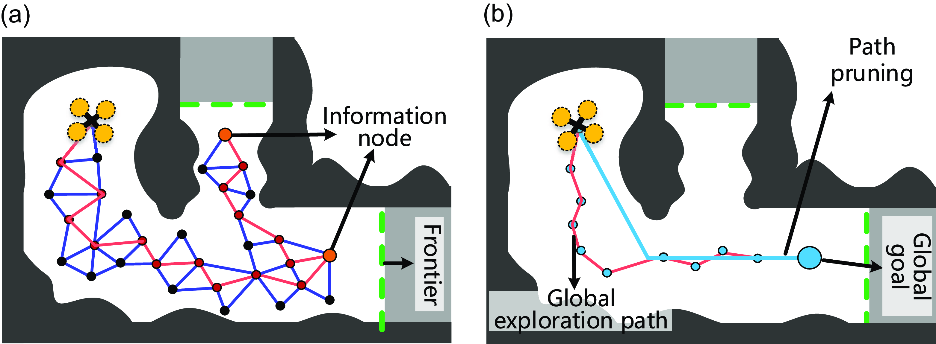
Global exploration stage. (a) The history graph and the information nodes. (b) The path pruning process of the global exploration path at the current iteration.

4.4. Global exploration stage
Similar to ref. [Reference Respall, Devitt, Fedorenko and Klimchik10], a sparse roadmap is continuously maintained during the MAV flight. The roadmap consists of sampled nodes and edges connecting these nodes. A node that contains the potential exploration information about its surrounding space is called information node. When there are no frontiers and uncovered surfaces within the local planning horizon, the planner turns to the global exploration stage, and the information nodes are used to guide the global exploration planning. As shown in Figure 5(a), the roadmap is continuously constructed during the MAV flight. The nodes of the roadmap contain two parts: the nodes directly sampled from the trajectory of the MAV (red solid circles) and the nodes sampled from the vicinity space around the MAV (black solid circles). The orange lines are the trajectory of the MAV, while the blue lines are the edges of the roadmap. When planning the global exploration path, the roadmap can efficiently return a feasible path towards any information node. However, the global exploration path may be tortuous and not appropriate for the MAV tracking. As shown in Figure 5(b), the path will be pruned to avoid detours and reduce the path length.
5. Results
5.1. Implementation details
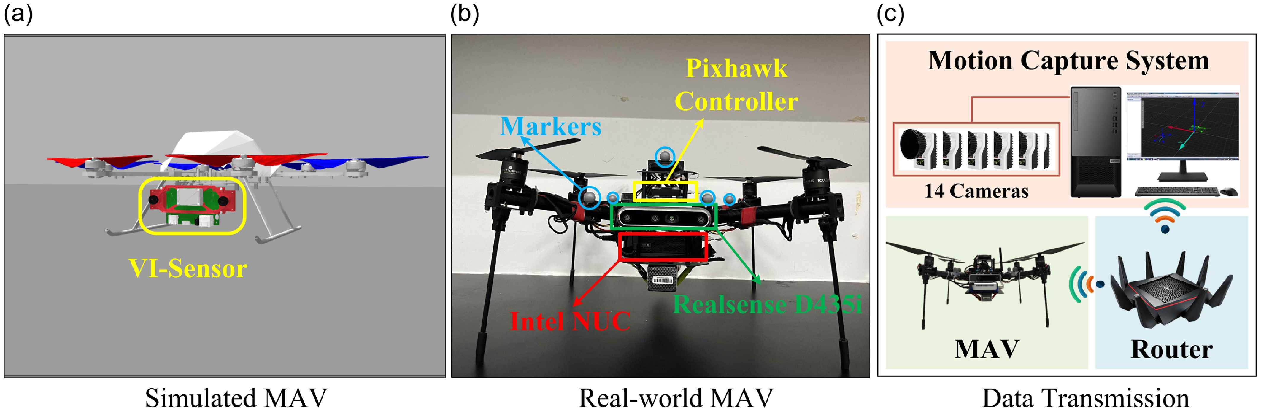
We first conduct benchmark evaluations in a realistic simulator, Gazebo [35], since it can provide realistic simulation environments and robot models. As shown in Figure 6(a), a forward-looking depth sensor is mounted on the MAV provided by the open-source library, Rotors [Reference Furrer, Burri, Achtelik and Siegwart36]. It has a min/max sensing range of
 $\left [ 0.5\;m,5\;m \right ]$
and field of view of
 $\left [90^\circ ,110^\circ \right ]$
in the vertical and horizontal directions. We design two complex scenarios (see Figure 7), Villa1 (
 $\textrm{} 24\, m \times 20\, m \times 10, m$
) and Villa2 (
 $ 29 m \times 25 m \times 12 m$
), in Gazebo for the benchmark comparison. To achieve fair evaluations, we implement all algorithms on the same computer, which was configured with an AMD Ryzen 7 3700 CPU and 16-GB memory. The operating system is Ubuntu Linux 18.04 LTS, and the corresponding ROS version is Melodic. In all trials, the resolution
 $r$
of TSDFs and ESDFs is set to
 $0.1$
 $m$
. The maximum linear velocity and the maximum yaw rate of the MAV are set to
 $1.5$
 $\textrm{}m/s$
and
 $1.0$
 $\textrm{}rad/s$
. In order to improve the surface coverage quality, we set
 $\theta _{\max } = 60^\circ$
in Eq. (5),
 $d_{\textrm{}min} = 1$
 $m$
and
 $d_{\textrm{}max} = 4$
 $\textrm{}m$
in Eq. (6), and
 $l = 10$
in Eq. (7). The rest of parameters are summarized in Table I.
Simulated and real-world robot platforms. (a) The simulated MAV is equipped with a forward-looking depth sensor, VI-Sensor. (b) The real-world MAV is equipped with a Pixhawk controller, a forward-looking Intel Realsense D455 sensor, and an Intel NUC computer. (c) The data transmission between the motion capture system and the real-world MAV is achieved through the local area network supported by a router.

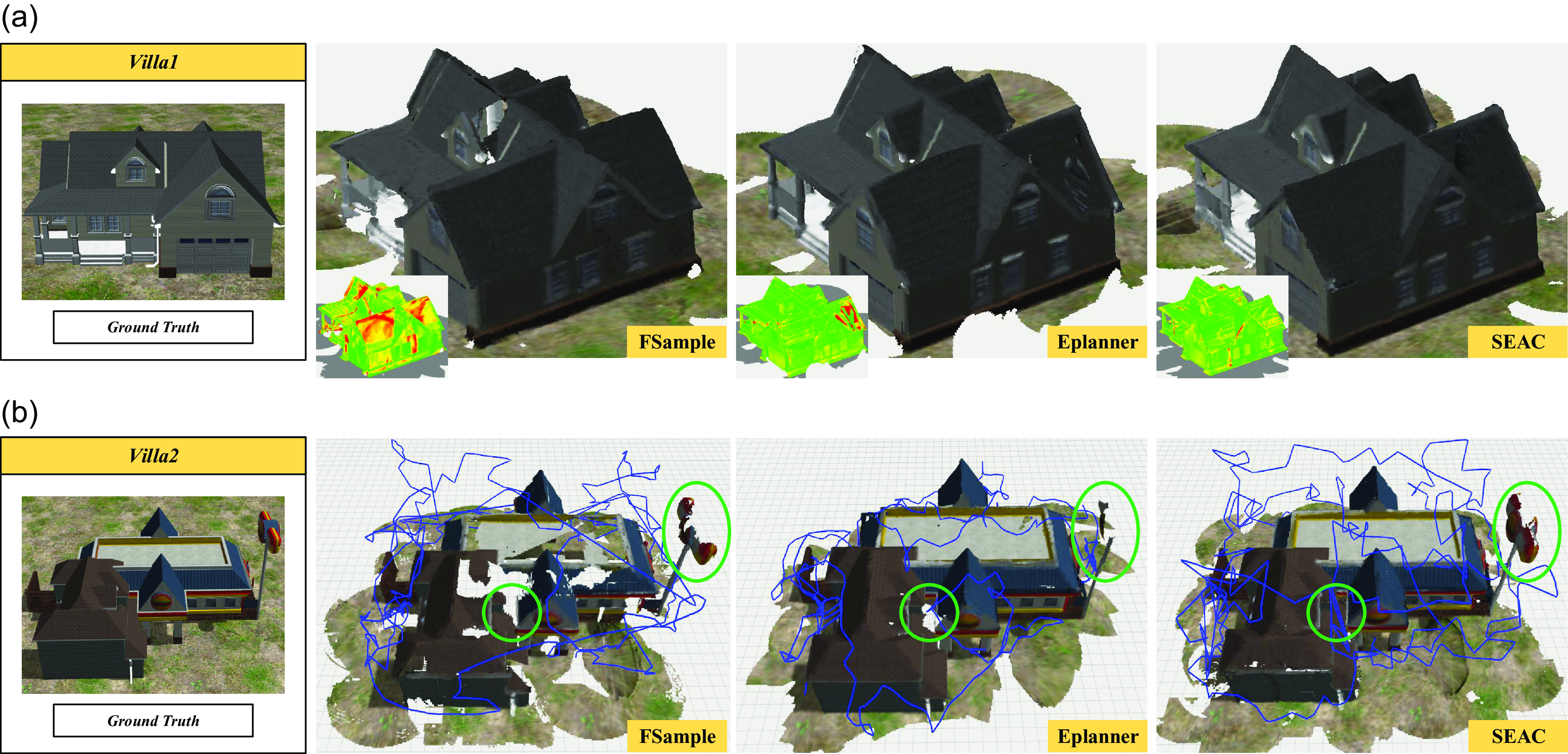
Reconstruction results of the benchmark comparisons. (a) The obtained 3-D Models of Villa1 and their corresponding reconstruction error (left bottom, wherein red means high error and green means low error) after 600
 $s$
. Since our method focuses on inspecting the reconstructed surfaces with low coverage quality, we obtain a higher overall accuracy and a more homogeneous error distribution. (b) Qualitative comparison (Reconstructed 3-D models with executed trajectories) of SEAC, FSample, and Eplanner in Villa2 after 900
 ${}s$
. Our method achieves the fullest reconstruction of the target, leaving the fewest holes on the mesh surface.

Parameters used in the simulation experiments.

It is worth noting that, similar to ref. [Reference Schmid, Pantic, Khanna, Ott, Siegwart and Nieto26], we add quadratically-scaling Gaussian noise to the ground truth point cloud obtained from the simulator to account for perception uncertainties presented in the real-world scenes as follows:
 \begin{equation} {z_{sim}} = z + \text{N}\left ( { {\mu \left ( z \right ),\sigma \left ( z \right )}} \right ), \end{equation}
where
 $\text{N}\left (\right )$
denotes the normal distribution function,
 $z$
is the depth measurement, and
 $\mu$
and
 $\sigma$
are the mean and standard deviation of the noise, respectively. In our trials, we set
 $\mu \left ( z \right )$
 $=$
 $\sigma \left ( z \right )$
 $=$
 $0.0024$
 $\textrm{z}^2$
.
To further validate the effectiveness of SEAC, we also carried out a real-world experiment in a laboratory environment on-board an MAV. Our self-built MAV employed in the real-world experiment is shown in Figure 6(b). The MAV is equipped with an Intel Realsense D435i depth sensor for acquiring the environmental data and an Intel NUC computer with an Intel Core i7-8550U CPU for running the proposed algorithm. We localize the MAV by a motion capture system and control the MAV using the SE(3) control algorithm [Reference Lee, Leok and McClamroch31]. As shown in Figure 6(c), the motion capture system comprises fourteen cameras and a ground station computer. It measures pose information for the MAV by identifying markers attached to the MAV. The MAV receives pose measurements from the motion capture system through the local area network supported by a router. The control signals are computed by the NUC computer and transmitted to the Pixhawk controller via the ROS-based communication protocol. For the parameters, we set
 $\mathcal H$
 $=$
 $ \textrm{}3\, m \times 3\, m \times 3\, m$
. The other parameters used in the experiment are kept the same as those used in the simulation (see Table I).
5.2. Benchmark comparisons
We compare SEAC with the state-of-the-art methods for exploring or modeling unknown targets:
-
• FSample [Reference Respall, Devitt, Fedorenko and Klimchik10]: A method that combines the frontier-based and sampling-based strategies in a unified framework to achieve complete exploration of the environment.
-
• Eplanner [Reference Schmid, Pantic, Khanna, Ott, Siegwart and Nieto26]: A sampling-based method achieves global optimal decisions by continuously expanding a single trajectory tree, but only the coverage utility of the sampled viewpoints is mainly considered in each planing epoch.
Remark 1: FSample is a pure exploration method, while EPlanner is a state-of-the-art online 3-D modeling method that mainly considers the surface coverage quality in its planning. We select these two methods to demonstrate that SEAC takes into account both the coverage quality and the exploration efficiency. To achieve the statistical comparison, all algorithms are run five times in each scenario.
5.2.1. Villa1 reconstruction
The first trial utilizes the MAV to autonomously reconstruct the building Villa1 online. Since the termination criteria of the evaluated methods are different, we set the maximum run time of each method in this scenario to
 $600$
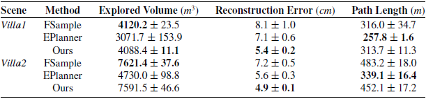
s. The comparison results of 5 runs are listed in Table II. In addition, Figure 7(a) shows the reconstructed 3-D models and the corresponding reconstruction error. It can be seen that FSample explored the largest volume of the environment (only 0.8% larger than SEAC) while resulting in the highest final reconstruction error (50.0% larger than SEAC). This is because FSample prioritizes maximizing the unknown volume that can be observed by the MAV in each iteration, while ignoring the reconstruction errors of the resulting 3-D model. By contrast, EPlanner explored the smallest volume of the environment and resulted in 31.4% larger reconstruction error than SEAC. This is because EPlanner primarily focuses on improving the surface coverage quality in each planning iteration, which leads the MAV to circle around the central building structure and, consequently, results in a low explored volume. It is worth noting that EPlanner has the shortest trajectory. The reasons are twofold. First, the computational cost for expanding and maintaining a single tree in large environments is high, which might cause the MAV to stay in place and wait for the planning result. Second, EPlanner focuses too much on the low-quality surfaces, thus neglecting to explore the unknown space. On the other hand, our method and FSample have the similar trajectory length as well as similar explored volume.
Result statistic of the benchmark comparisons.

5.2.2. Villa2 reconstruction
The second trial is to reconstruct Villa2. Since this scenario is larger and more complex than Villa1, we set the maximum run time of each method to
 $900$
s. As shown in Table II, the results of this scenario are similar to the first one. Figure 7(b) shows the reconstructed 3-D models with the executed trajectories. Specifically, FSample explored the largest volume of the environment (only 0.4% larger than SEAC) while resulting in the highest reconstruction error (46.9% larger than SEAC). Similarly, EPlanner explored the smallest volume of the environment and resulting in 14.3% larger reconstruction error than SEAC. In addition, EPlanner exhibits the shortest trajectory, whereas our method and FSample demonstrate longer trajectories.
5.2.3. Computational time
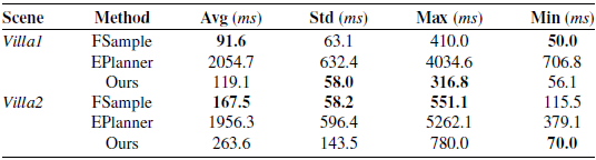
As shown in Table III, we recorded the computational time for each planning iteration of each method used. It can be seen that the mean computational time of our method and FSample is an order of magnitude less than that of EPlanner. This is because FSample maintains a large single tree during each iteration for computing the globally optimal informative path, which is inherently expensive as it has to evaluate all the candidates to guarantee global optimality. On the contrary, both our method and FSample compute the MAV path within a local planning horizon and thus can reduce the computational time significantly. When comparing our method with FSample, we find that, despite FSample using slightly less time, their mean computational times are quite similar. The reason for our method taking more computational time is that it not only plans an exploration path but also further refines the path to enhance the coverage quality of the reconstructed surfaces.
Computation time used for each planning iteration.

In summary, our method not only achieves the highest overall reconstruction accuracy but also produces the most complete 3-D models, leaving the fewest holes on the mesh surface. Moreover, our method is computationally efficient, which enables it to be used on resource-limited MAVs.
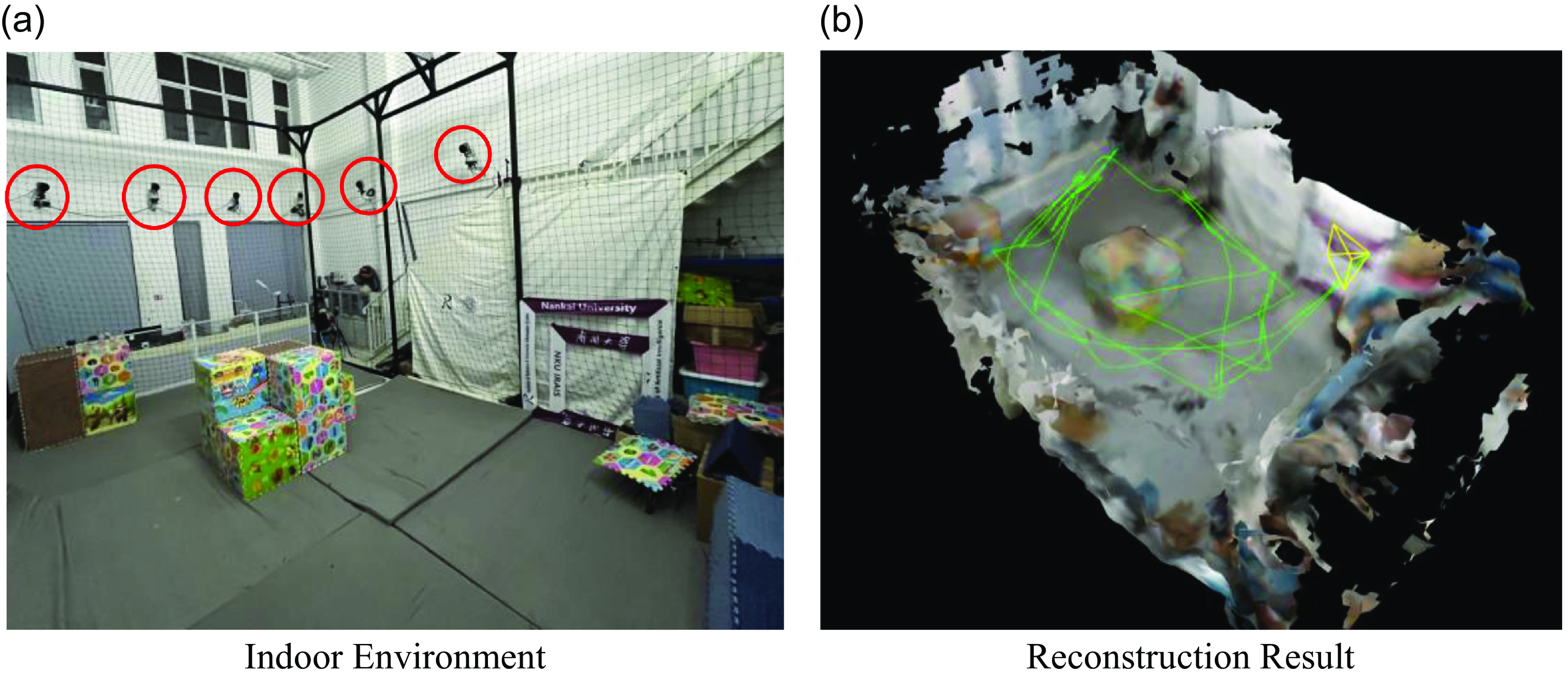
Reconstruction result of the indoor experiment. (a) The configuration of the indoor environment includes a motion capture system made up of 14 cameras (as shown in the red circles). (b) The 3-D model of the indoor experiment is reconstructed by our method, and the green line represents the executed trajectory of the MAV.

5.3. Real world experiment
In this section, we present the experiment for online 3-D modeling of an indoor environment (see Figure 8 (a)) by using our sefl-built MAV (see Figure 6 (b)). This size of the indoor environment is
 $\textrm{}7.0\, m \times 4.2\,m \times 2.5\, m$
. In the experiment, we set the min/max sensing range of the Intel D435i sensor as
 $\left [ 0.2\;m,3.5\;m \right ]$
and the field of view as
 $\left [58^\circ ,87^\circ \right ]$
. The maximum linear velocity and the maximum yaw rate of the real MAV are set to
 $1.0$
 $\textrm{}m/s$
and
 $0.5$
 $\textrm{}rad/s$
. According to the experiment result, our method can complete the online 3-D modeling task in 165
 $s$
and thus obtain almost complete environmental surfaces. The mean computational time used for each planning iteration is 288.0
 $\textrm{}ms$
, with a standard deviation of 134.7
 $\textrm{}ms$
, demonstrating the online performance of SEAC. The average length of the MAV’s trajectories over five runs is 59.5
 $\textrm{}m$
, with a standard deviation of 4.5
 $m$
. The reconstructed 3-D model of the representative run is shown in Figure 8 (b), in which the green line is the executed trajectory of the MAV.
More details of the benchmark comparisons and the real-world experiment can be found at https://youtu.be/Y23AMLUHxBU.
6. Conclusions
This paper proposes a novel online informative path planner for simultaneously exploring and covering unknown 3-D structures. Our method can achieve accurate online 3-D reconstruction without any prior information or offline processing. Specifically, we first devise a set of efficient metrics for evaluating the coverage quality of the reconstructed surfaces, which can facilitate the utility calculation of candidate viewpoints. Then, a hierarchical planner is proposed to cover the entire target by switching between local coverage stage and global exploration stage. The local coverage stage generates local coverage paths for inspecting surfaces with low coverage quality, and the global exploration stage is to output global exploration paths for global exploration. We compared our method with existing algorithms in two challenging scenarios. The results show that our method is capable of significantly reducing the reconstruction error and producing complete 3-D models. Finally, the real-world experiment demonstrated that our method can be run onboard a real MAV.
The main limitation of our method is that we evaluate it using ground-truth localization, whereas in physical environments, localization errors cannot be ignored. In future work, we aim to further investigate SEAC for online 3-D modeling in scenarios suffering severe odometry drifts. Furthermore, existing literature, as well as our work, primarily relies on simulations or simple qualitative experiments for validating the 3-D modeling performance. Therefore, it is also crucial to design an effective strategy for the quantitative evaluation of SEAC methods in real-world scenarios.
Author contributions
Shiyong Zhang, Xuebo Zhang, and Qianli Dong designed the planner and conducted the code implementation. Qianli Dong, Tianyi Li, and Haobo Xi conducted the simulation comparisons and data gathering. Shiyong Zhang and Ziyu Wang conducted the real-world experiment. Shiyong Zhang, Xuebo Zhang, Chaoqun Wang, and Jingjin Yu wrote the article.
Financial support
This work was supported in part by Natural Science Foundation of China under Grant Number 62303249, in part by the China Postdoctoral Science Foundation-Tianjin Joint Support Program under Grant Number 2023T013TJ, and in part by the China Postdoctoral Science Foundation under Grant Number 2024M751526.
Competing interests
The authors declare no conflicts of interest exist.
Ethical approval
Not applicable.