I. Introduction
Growers face many questions in deciding which variety of winegrapes to plant, including choices about which clone among perhaps dozens available for a chosen variety. It is widely understood that different varieties can be expected to do better or worse in particular locations, depending on soil types, topography, and local climate—sometimes referred to as terroir. The value of the grapes produced will depend on these factors, in interaction with the market demands for wines having particular flavor profiles and other relevant characteristics, including the varietal name itself in some cases.
Varietal choices are made more difficult because the variety-by-location interactions that determine the value of a particular variety vary significantly over space (sometimes over very short distances) and time (sometimes over very short intervals). While differences in their terroir and economic history of wine have led to enduring systematic differences in the varietal mix among producing regions, changes in patterns of demand, and in the structure of the (increasingly internationally interconnected) global markets for wine, have contributed to systematic shifts in the varietal mix among locations on a shorter time scale. Actual or expected changes in climate also may have contributed.
One source of shifting emphasis on particular varieties is changes in the demand for wine, reflecting changes in population and income, and shifting preferences both among wines and between wines and other beverages. The globalization of the world's wine markets has encouraged wine consumers to seek new types of wines, and has generated many new wine consumers, while some traditional wine consumers have drifted to other beverages. Seeking to attract and retain consumer attention, producers differentiate their products. Traditionally the Old World emphasized regional differences and restricted both the range of varieties grown in each region and the use of varietal labelling on bottles (see, e.g., Gaeta and Corsinovi, Reference Gaeta and Corsinovi2014). In contrast, in the United States and other New World countries differentiation has been mainly through varietal labeling, although gradually more emphasis is being given also to regional and even single-vineyard labeling.
Another source of shifting varietal emphasis is changes on the supply side. The observed mix of grape varieties reflects judgement by vignerons about what is best to grow in their region. That judgement is affected not only by terroir but also by past and present economic considerations, including expectations about future price trends and the cost involved in grafting new varieties onto existing rootstocks or grubbing out and replacing existing varieties. Climate changes (higher temperatures, more extreme weather events) mean that the structure of the variety-by-location relationships is changing (see, e.g., Ashenfelter and Storchmann, Reference Ashenfelter and Storchmann2016), and they are causing changes in comparative advantages even in places not affected directly, since it is a worldwide phenomenon and a global marketplace. Producers are well aware of the impacts climate changes are having on their winegrapes. Adaptation strategies include switching to warmer-climate or more-resilient grape varieties, and sourcing more from regions with a higher latitude or altitude or closer to the sea. Especially in regions and sites whose varietal comparative advantages are still unclear, winegrowers are continually searching for varieties that do well in climates similar to what they expect theirs to become in the future.
Are places becoming more similar, reflecting a shared incentive to shift towards currently more-generally favored varieties? Or are they becoming more differentiated, reflecting better-linked markets and more clearly defined comparative advantage? What role is played by the demand for a complete portfolio of varietal wines from a particular region, regardless of sub-regional comparative advantages in every other sense? To address such questions requires detailed information on what winegrape varieties are grown where, and how those patterns are changing.
Recently, Anderson and Aryal (Reference Anderson and Aryal2013) compiled a global database for 2000 and 2010 to serve these broad purposes.Footnote 1 This paper draws on that newly compiled global database plus additional new U.S. data to generate several indicators that capture recent changes in the varietal mix in the United States and its wine regions vis-à-vis the rest of the world. Regional and varietal shares of national and global bearing area and production of winegrapes are reasonably straightforward measures to compute and interpret when data are available—subject to the vagaries of varietal names as discussed and addressed satisfactorily by Anderson and Aryal (Reference Anderson and Aryal2013) by adopting the prime names chosen by Robinson et al. (Reference Robinson, Harding and Vouillamoz2012) and listed in the online supplementary Appendix Table B-3. We report these measures for various aggregates. In addition, we use several other indexes as used by Anderson (Reference Anderson2014): (a) a varietal intensity index (VII), (b) a varietal similarity index (VSI), and, using winegrape price as a proxy for quality, (c) a regional quality index (RQI) and (d) a varietal quality index (VQI). The online supplementary Appendix B provides detail on the data used to compute these indexes.
The paper is structured as follows. Section II provides an overview of the U.S. wine industry and its economic geography and relevant history. This provides a foundation for the subsequent discussion of the regional-cum-varietal structure of production. A set of empirical pictures of the changing varietal distinctiveness of U.S. wine regions is presented in Section III. Section IV then analyzes regional and varietal quality differences within the United States, as reflected in winegrape prices. Section V presents a more formal statistical analysis of the role of measures of economic incentives in the evolving production patterns. The final section summarizes and synthesizes the findings and concludes the paper.
II. An Overview of U.S. Wine Production Regions
The U.S. wine industry is young by Old World standards, especially in its current incarnation that began to develop after 13 years of Prohibition, which ended in 1933. As in the rest of the New World, during recent decades the U.S. wine industry has grown rapidly: production has increased by about 75% since 1980. These and other changes took place in the context of some fundamentals that remained largely constant and determine the regional patterns of comparative advantage that favor wine production on the West Coast, especially in California (see, e.g., Lapsley, Reference Lapsley1996; Sumner et al., Reference Sumner, Bombrun, Alston, Heien and Anderson2004; Olmstead and Rhode, Reference Olmstead, Rhode, García Ruiz, Andreu, Critz, José and Ortiz-Villajos2010).
In 2010, the United States produced 3.7 million tons of grapes crushed for wine, with a farm value of $2.3 billion—representing about 10% of the world's wine volume. Of the U.S. total winegrape area of 228 thousand hectares in 2010, four states accounted for over 96%: California (CA), 79.7%; Washington (WA), 7.8%; New York (NY), 5.6%; Oregon (OR), 3.0%. Of these, only New York is not on the West Coast. In 1990, California alone accounted for 88.1% of the total and New York accounted for 8.9%. In the 20 years since, while the total U.S. winegrape area increased by about 50%, the winegrape area shrunk slightly in New York while growing rapidly in Oregon (four-fold) and Washington State (six-fold). California differs from the other major producing states, and itself contains several distinct wine production regions that differ in terms of their terrain, climate, soil types, mixture of varieties grown, and quality of grapes and wines produced. Data on production and prices of winegrapes in California are available in some cases by county (of which there are 58, not all of which grow wine grapes) and in others by crush district (of which there are 17). Some crush districts contain several counties or parts of counties.
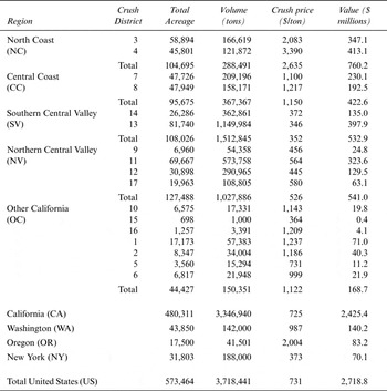
In this paper we use data for California on the basis of crush districts, in some cases derived from data that were originally available on the basis of counties, which requires some assumptions if counties are divided across crush districts. But for most of the work we aggregate the crush districts into five regions, defined such that each county fits entirely into one of the five regions (see online supplementary Appendix Table A-1 and Appendix Figure A-1 for details).Footnote 2 Treating each of the other significant wine-producing states (i.e., WA, OR, and NY) as a region, we have eight primary U.S. wine-producing regions comprising these three plus the five in California. We have more-complete information on the industry in the West Coast states, and some of our detailed analysis is restricted to these three states. Table 1 includes some detail on the salient features of the eight main U.S. wine-producing regions we have identified.
Characteristics of U.S. Winegrape Growing Regions, 2011 Data

Sources: Created by the authors using data from USDA NASS historical crush reports, available at http://www.nass.usda.gov/Statistics_by_State/California/Publications/Grape_Crush/index.asp, and USDA NASS historical acreage reports, available at http://www.nass.usda.gov/Statistics_by_State/California/Publications/Grape_Acreage/index.asp.
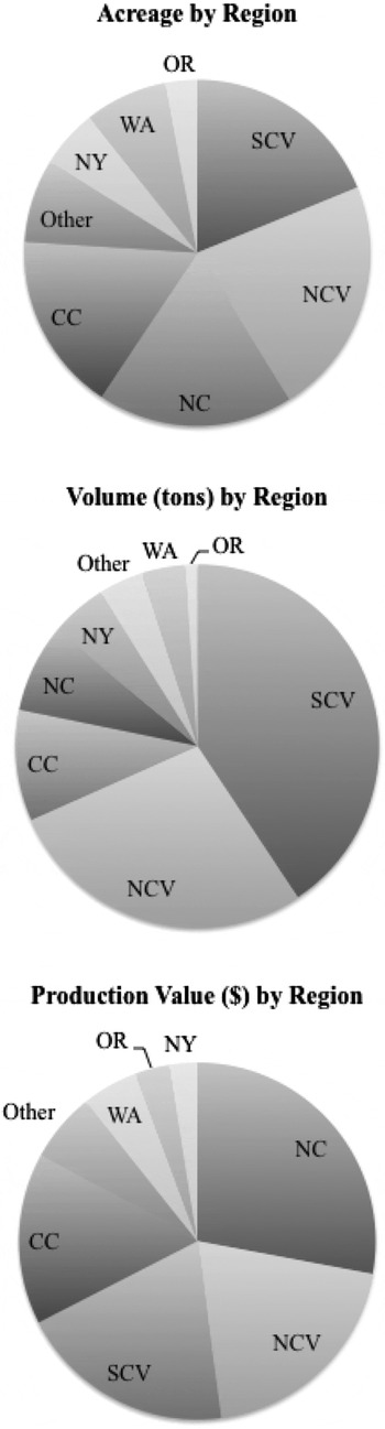
Several distinct patterns are apparent as illustrated in Figure 1. First, California dominates the national total area, volume and value of wine production. Second, the regional shares differ significantly among measures of area, volume, and value of production. In particular, the Southern Central Valley has a much larger share of volume compared with area and especially value of production, while the North Coast region (mainly Napa and Sonoma) has a much smaller share of volume compared with area and value of production. These patterns reflect the relatively high yield per acre (and correspondingly low price per ton) of grapes from the Southern Central Valley and the conversely low yield and high price per ton in the North Coast.
U.S. Wine Regions—Area, Volume, and Value of Production, 2011

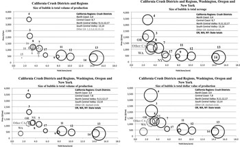
Figure 2 illustrates graphically the links between the price per ton, yield per acre, and the implications for shares of value and volume of production of winegrapes across U.S. regions (and crush districts within regions in California). In 2011 in the Napa Valley the average yield was 2.7 tons/acre and the average crush price was $3,390/ton, almost ten times the average crush price in the Southern Central Valley where the average yield was over 14 tons/acre. The other regions were distributed between these extremes in a nonlinear fashion but with higher yields generally associated with lower prices per ton. Within regions, yields and prices are determined in part by the choice of varieties grown.
U.S. Wine Regions—Average Yield, Price, and Shares of Area, Volume, and Value, 2011

III. Varietal Distinctiveness of U.S. Wine Regions
In what follows, we examine the patterns of varietal choice and quality as they vary among regions and over time. First, we examine the varietal distinctiveness of vineyard plantings in the United States vis-à-vis the rest of the world, the varietal differences among regions within the country and their changing varietal intensities.
A. Global and U.S. varietal distributions
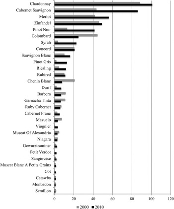
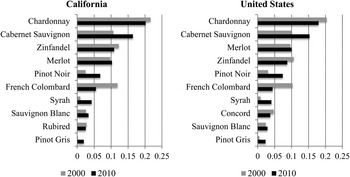
As a starting point, consider the range of varieties grown. Anderson (Reference Anderson2014, Figure 3b) plots the shares of global bearing area for the world's top 35 wine varieties (by bearing area) in 2010, compared with 1990 and 2000. These 35 varieties accounted for 66 percent of the total bearing area in 2010. This figure (a variant of which is provided in the online supplementary Appendix Figure A-2) illustrates the enormous (but changing) diversity of global winegrape production while also showing the relative importance of the top 10 varieties, which accounted for 42 percent of the global total bearing area in 2010. Figure 3 is the U.S. counterpart: it plots the shares of U.S. bearing area for the top 30 U.S. wine varieties in 2010, compared with 1990 and 2000. The top 30 U.S. varieties accounted for 92.7 percent of the total U.S. bearing area in 2010, and the top 10 varieties accounted for 76.5 percent.
Top 30 U.S. Winegrape Varieties in 2010, Compared with 2000 (bearing acres)

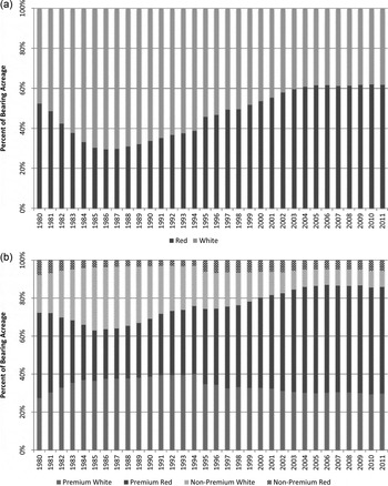
Figure 4 plots the evolving U.S. varietal mix over the past thirty years. The varietal mix has drifted toward red and away from white varieties (Panel a), and for both red and white varieties toward premium varieties (Panel b)—particularly Chardonnay, Cabernet Sauvignon, Merlot, Pinot Noir, and Syrah (see online supplementary Appendix Figure A-3).Footnote 3 In the most recent decade or so, in particular, the picture is dominated by increased plantings of popular premium red and white varieties (in rank order: Cabernet Sauvignon, Pinot Noir, Syrah, Merlot, Chardonnay, and Pinto Gris), at the expense of less-favored varieties (in rank order: French Colombard, Chenin Blanc, Barbera, and Grenache) (see online supplementary Appendix Figure A-4).
California Varietal Shares of Bearing Acreage, 1980–2011

B. Regional differences within the United States
Within the United States, five varieties (Chardonnay, Cabernet Sauvignon, Merlot, Pinot Noir, and Zinfandel) accounted for 51.8 percent of the total volume and 65.6 percent of the total value of production in 2011.Footnote 4 These five varieties predominate in several of the main production regions—in particular in the premium price regions within California, as well as in Washington and Oregon—but the emphasis varies among the premium price regions and some regions are quite different. In particular, the hot Southern Central Valley (dominated by French Colombard and Rubired used to produce grape juice concentrate as well as bulk wine) and New York (dominated by non-vinifera American varieties, Concord and Niagara) are quite unlike the other regions climatically and in terms of their grape varietal mix (see online supplementary Appendix Figures A-5 and A-6).Footnote 5
Chardonnay is the most important variety in terms of total bearing area nationally and is highly ranked throughout the premium regions, but the Napa-Sonoma region is especially known for its Cabernet Sauvignon, which is its most important variety and increasingly so, and likewise in Washington. The cooler coastal regions—in particular Oregon and the Central Coast of California—are relatively specialized in Chardonnay and Pinot Noir and other cool climate varieties. Zinfandel is more significant in the Northern Central Valley and other mid-price regions, and these patterns reflect this variety's dual roles in serving as both a premium red varietal wine and as a bulk “blush” (white zinfandel) wine.
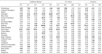
Anderson (Reference Anderson2010) defined the Varietal Intensity Index, VII im for variety m in region i as:
 $$VI{I_{im}} = {\,f_{im}}/{f_m}.$$
where f
m
is the bearing area of grape variety m as a proportion of the total global bearing area of winegrapes, and f
im
is the bearing area of grape variety m in region i, as a proportion of the total bearing area of winegrapes in that region, 0 ≤ f
m
, f
im
≤ 1 and
 $\sum {f_m = \sum f} _{im} = 1$
. When region i is relatively specialized in production of variety m, compared with the world as a whole, VII
im
> 1. Table 2 shows VIIs for the main varieties in the U.S. wine regions, the main states, the United States as a whole and, for comparison, Australia and France. The indexes in Panel a refer to 2010. Indexes greater than 3 are in bold face.
U.S. Wine Regions: Varietal Intensity Indexes, 2010

Notes: Varieties are ranked in order of 2011 U.S. total acreage. California regions are North Coast (NC), Central Coast (CC), Northern Central Valley (NV), Southern Central Valley (SV), and Other California (OC). States are California (CA), Washington (WA), Oregon (OR) and New York (NY). VII is calculated using bearing acreage data from Anderson and Aryal (Reference Anderson and Aryal2013).
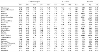
U.S. Wine Regions: Varietal Intensity Indexes, 2000

Notes: Varieties are ranked in order of 2011 U.S. total acreage. California regions are North Coast (NC), Central Coast (CC), Northern Central Valley (NV), Southern Central Valley (SV), and Other California (OC). States are California (CA), Washington (WA), Oregon (OR) and New York (NY). VII is calculated using bearing acreage data from Anderson and Aryal (Reference Anderson and Aryal2013).
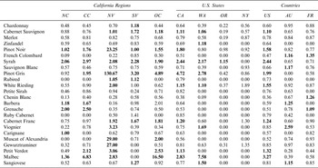
U.S. Wine Regions: Varietal Intensity Indexes, Ratio of 2010 VII to 2000 VII

Notes: Varieties are ranked in order of 2011 U.S. total acreage. California regions are North Coast (NC), Central Coast (CC), Northern Central Valley (NV), Southern Central Valley (SV), and Other California (OC). States are California (CA), Washington (WA), Oregon (OR) and New York (NY). Source: Created by the authors using data from Anderson and Aryal (Reference Anderson and Aryal2013).
In some instances particular regions have very high VIIs for particular varieties. Whether these high VIIs are reflected in the state and national counterpart measures depends on the size of the regions and the extent to which they differ from other regions. The Southern Central Valley (SV) of California is a comparatively large producing region, with a distinctive varietal mix used for producing bulk wine and grape juice concentrate. In that region, the VII for Rubired is huge (VII sv = 100.80), indicating that in that region the share of Rubired in winegrape area is over 100 times the share of Rubired in the global winegrape area. The counterpart index for California is over 25, and for the nation over 20, even though Rubired is not grown outside California's Central Valley. The Southern Central Valley is also comparatively highly specialized in French Colombard (VII sv = 30) and Ruby Cabernet (VII sv = 38), to an extent that makes the state and national VIIs large for these varieties, too. Every region of California is highly specialized in Zinfandel compared with the world as a whole (VII US > 12). In the case of Petite Sirah, every California region except the Southern Central Valley has a large VII and consequently so do California and the nation as a whole. By global standards, the United States is comparatively specialized in Chardonnay (VII US > 4) and Cabernet (VII US > 2), and this is reflected in the VIIs in most regions (except New York, Oregon, and the Southern Central Valley). Washington is comparatively specialized in White Riesling while Oregon is comparatively specialized in Pinot Noir and Pinot Gris.
U.S. Wine Regions—Top 10 Varieties, Share of Bearing Acreage, 2000 and 2010

Comparing panels a and b of Table 2 reveals the shifts in varietal intensities between 2000 and 2010. In many instances, the bold entries in panel a (for 2010) are smaller than their counterparts in panel b (for 2000) indicating that the particular region has become less specialized, comparatively, in that variety. But in some cases the opposite is true. To clarify the comparison, in panel c each entry is the ratio of the VII for 2010 to its counterpart for 2000: that is, VIIR im = VII im(2010)/VII im(2000). If a ratio is greater than 1.0, it is shown in boldface. The majority of the entries are not bold but some are, indicating an increase over that decade in VII. The United States (in particular in the premium regions of California and Washington and Oregon, depending on the variety) has increased its relative specialization in production of some varieties in which it was already somewhat specialized—such as Cabernet Sauvignon and Pinot Noir—as well as some in which it was not, namely Syrah, Pinot Gris, Pinot Noir, Petit Verdot, Cabernet Franc, White Riesling, and Malbec. But France and Australia, by contrast, have tended to become less specialized in the varieties in which they were comparatively specialized.
C. National and regional varietal distinctiveness
Anderson (Reference Anderson2010) defined a Varietal Similarity Index (VSI) as:Footnote 6
 $$VSI_{v,t} = \displaystyle{{\sum\limits_{m = 1}^M {\,f_{i,m} f_{\,j,m}}} \over {\left( {\sum\limits_{m = 1}^M {\,f_{i,m}^2}} \right)^{1/2} \left( {\sum\limits_{m = 1}^M {\,f_{\,j,m}^2}} \right)^{1/2}}}. $$
This index can be used to measure the extent to which the winegrape varietal mix of one region or country, i matches that of another region or country (or the world), j. It can also be used to compare the varietal mix of a region or country over time. This index is conceptually similar to a correlation coefficient and, like a correlation coefficient, it is completely symmetric in that VSI i,j = VSI j,i and VSI i,i = 1.
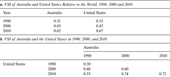
The VSI between the United States and the world was 0.15 in 1990 but it rose to 0.42 in 2000 and 0.67 by 2010, indicating a very substantial drift in the U.S. varietal mix toward the world aggregate mix (Table 3, Panel a). Over the same period, the VSI between Australia and the world rose from 0.31 in 1990 to 0.43 in 2000 and 0.62 by 2010 (Anderson, Reference Anderson2015). By this measure, in 1990 the mix of winegrape varieties in both the United States and Australia drifted toward the world aggregate mix, but the U.S. mix moved more: it was much less similar than the Australian mix to the world aggregate in 1990 (0.15 versus 0.31) but by 2010 it was more similar (0.67 versus 0.62). And the mixes in Australia and the United States today are much more similar than they were in 2000 and especially 1990 (Table 3, Panel b). These same developments are illustrated graphically by Anderson (Reference Anderson2014, Figure 6 pp. 14–15; a variant of which is replicated as online supplementary Appendix Figure A-7. Since France is the country whose varietal mix is most similar to the world mix, this means in effect that the United States has become more like France.
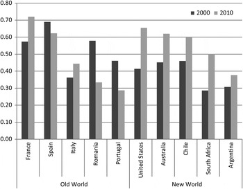
Index of Varietal Similarity Between World and Five Largest Old World and New World Wine-Producing Countries, 2000 and 2010

Winegrape Varietal Similarity Indexes: United States, Australia and the World

Source: Anderson and Aryal (Reference Anderson and Aryal2013), Anderson and Aryal (Reference Anderson and Aryal2014).
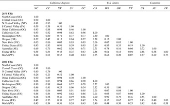
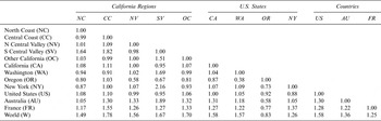
Table 4 includes VSIs among U.S. regions relative to one another, and relative to U.S. states, as well as Australia and the United States. The upper half of the table refers to VSIs in 2010 and the lower half refers to 2000. Between 2000 and 2010, the United States wine industry became more like the global wine industry: VSI US,WORLD increased from 0.42 to 0.67. This reflected a global trend—France and Australia also became more like the global wine industry, but did not adjust by as much as the United States did (VSI FR,WORLD increased from 0.58 to 0.73, reflecting in part the predominant role of France in the global total, andVSI AU,WORLD increased from 0.46 to 0.62). The U.S. adjustment reflected every U.S region becoming more like the global industry, in terms of its varietal mix, with two exceptions: Oregon (highly specialized in Pinot Noir) and New York (growing American varieties) became more dissimilar. Setting aside these two states, within the United States, the more premium regions (North Coast, Central Coast, Other California, and Washington) tend to have varietal mixes quite similar to one another (i.e., VSI > 0.8) and reasonably similar to the world as a whole (i.e., VSI > 0.6), whereas the regions specializing in bulk wines and grape juice concentrate are quite dissimilar to the other U.S. regions and to the world as a whole with VSIs < 0.5.
Varietal Similarity Indexes for U.S. Regions, Australia, France, and the World

To highlight the changes between 2000 and 2010, the entries in Table 5 were computed by dividing each entry in the upper part of Table 4 (for 2010) by its counterpart in the lower part (for 2000): i.e., VSIR ij = VSI ij(2010)/VSI ij(2000). The resulting ratio of indexes will be greater than 1 if the index has increased (i.e., the varietal mixes have become more similar) over time. As can be seen in Table 5, the predominant pattern is for the indexes to increase—though not in every instance—and some of the increases are quite substantial. Figure 6 captures the key patterns for the five largest wine producing countries from the New World and the five largest from the Old World. The New World producers have become more like the world as a whole while the Old World producers have become less so, partly because the New World producers have become more important within the total.
Varietal Similarity Index Ratios, 2010:2000 for U.S. Regions, Australia, France, and the World

Source: Created by the authors using data from Anderson and Aryal (Reference Anderson and Aryal2013).
IV. Regional and Varietal Quality Differences within the United States
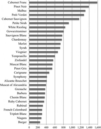
That U.S. winegrape regions vary substantially in terms of average winegrape prices received by growers is apparent from the plots in Figure 1. Given that different varieties grow better in some regions than others, and that consumer preferences differ across varieties and over time, it is not surprising to find considerable dispersion in the national average prices by variety. Figure 7 shows the U.S. average prices for the top 30 varieties in 2011, ranging from a little over $200 per ton for Burger to almost $1,600 per ton for Cabernet Sauvignon: an almost ten-fold difference across all varieties. These national average prices mask differences among regions and within regions—especially in the premium regions such as the North Coast, within which prices for a given variety can vary quite widely.
Average Price of Winegrapes, Top 30 Varieties, United States, 2011 in US$ per ton

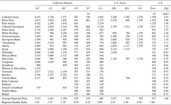
We use relative prices as an indicator of quality, comparing different varieties of winegrapes from different producing regions. Table 6 includes information on crush prices for winegrapes in 2010 by region for the top 25 varieties, for individual U.S. regions, states, and the nation as a whole. The last entry in each column of Table 6 is the Regional Quality Index (Anderson Reference Anderson2010), defined as the regional average winegrape price (across all varieties), P i in region i, as a proportion of the national average winegrape (across all varieties and all regions), P:
 $$RQI_i = P_i /P.$$
U.S. Regional and Varietal Winegrape Prices and Quality Indexes, 2010

The last entry in each row of Table 6 is the Varietal Quality Index, VQI m (Anderson Reference Anderson2010), defined as the ratio of the national average price for a particular variety across all regions, P m for variety m, to the national average price of all winegrape varieties:
 $$VQI_m = P_m /P.$$
The entries in Table 6 are sorted according to this index, so they are ranked from highest to lowest average VQI.
As can be seen in Table 6, prices vary systematically among regions—the North Coast region has generally higher prices than other regions for all varieties and the Southern Central Valley has generally lower prices. In addition, prices vary systematically among varieties—among the higher-quality (higher-priced) varieties grown in significant quantity, Cabernet Sauvignon generally is ranked higher than Chardonnay, and Zinfandel generally is ranked lower. But the sizes of the premia, and even the rankings of varieties, vary among regions. For example, Pinot Noir ranks above Cabernet Sauvignon almost everywhere, but not in Oregon where Pinot is by far the dominant variety, nor in the North Coast region; Chardonnay is ranked above Cabernet Sauvignon in the Central Coast region.
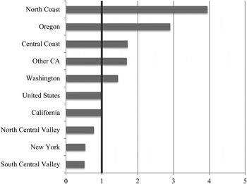
The Regional Quality Indexes (RQIs) plotted in Figure 8 are all relative to the national average of 1. The Central Valley of California produces a large volume of lower quality grapes (RQIs of 0.52 and 0.78 in the southern and northern regions) and, as a result, the average quality for California is slightly below the national average even though California also produces most of the national volume of higher-quality winegrapes. Among other states, consequently, only New York ranks below California in this measure. But the North Coast region stands out from the rest, with an RQI of 3.95, followed by Oregon at 2.91.
Regional Quality Index, United States, 2011

Some insight into the region-by-variety interactions is gleaned by considering the variety-specific panels in online supplementary Appendix Figure A-8. For each of the top 12 U.S. varieties (ranked according to 2011 bearing acreage), we have plotted the Varietal Quality Index (VQI) for each of our eight regions (i.e., five California regions, plus the three other states: Oregon, Washington, and New York), with the regions ranked according to the VQI. As one would expect, for many of the varieties the North Coast has the highest VQI, and it is often followed by Oregon for the premium varietals, but not always. The ranking and the size of the dispersion below the top varies considerably—compare Zinfandel and Pinot Noir.
V. Statistical Analysis of the Evolving Varietal and Quality Mix
The changing patterns of production reflect producer investments and their other production decisions made in response to their perceptions of the evolving market for winegrapes, taking into account their expectations about regional-cum-varietal comparative advantage over the relevant planning horizon, which can amount to decades in the case of winegrapes. Modeling supply response of perennial crops is challenging, and in the case of winegrapes is made more difficult by the highly differentiated nature of the product both within and among regions (see, e.g., Volpe et al., Reference Volpe, Green and Heien2011 and Alston et al., Reference Alston, Fuller, Kaplan and Tumber2013). Here, while we do not propose a formal supply response model as such, we draw on the relevant literature to develop statistical models of the influences of readily observable economic variables on production patterns. The same ideas were implicit in our graphical analysis.
Our measure of regional comparative advantage, for a particular variety, v, is given by the average revenue per acre (i.e., average yield in tons per bearing acre times average price in dollars per ton) of that variety relative to the average revenue per acre of all varieties in the same region:Footnote 7
 $$\pi _{v,t} = \displaystyle{{P_{v,t} Y_{v,t}} \over {\bar P_t \bar Y_t}}. $$
Given the durable nature of vineyards, the current pattern of production might depend on expectations formed 10 or 20 years (or more) previously, and we should not expect to see large shifts in production, in a particular location, in response to contemporary or even recent changes in the values of this incentive variable. On the other hand, enduring differences in the varietal mix among locations ought to reflect enduring differences in these incentives, and significant shifts in production patterns over time should reflect changes in expectations that we would expect to be related to systematic changes in incentives.
We exploit variation in varietal production patterns, both over time and across regions of California, as they relate to this measure of incentives, with some allowance for lagged responses. The general form of the model we have in mind is one in which the “desired” variety-specific share of total vineyard area (including non-bearing area) in a particular region, R, is a function of expected relative profitability over the indefinite future, which we proxy using lagged values of the measure of comparative advantage given in equation (5), allowing for fixed effects of variety and year, as follows:
 $$\ln \left( {\,f_{v,t}^ {\ast}} \right) = \beta _0^R + \sum\limits_{v = 1}^V {\beta _v^R} D_v + \sum\limits_{t = 1}^T {\beta _t^R} D_t + \beta _\pi ^R \ln \left( {\pi _{v,t}^e} \right) + \varepsilon _{v,t.} $$
In this model in region R, f v,t is the share of total acreage planted to variety v in year t, and the asterisk denotes the desired value that would maximize the producers' objective function; D v and D t are dichotomous (0–1) indicator variables to represent the effects of variety and year-specific fixed effects; and ɛ v,t is a random error term. The incentive variable, π v,t , is a measure of the relative profitability (or regional comparative advantage) of variety v in year t, as given in (5), and the superscript e denotes the expected value of that incentive variable. Since the model is specified in natural logarithms, the parameters are elasticities.
We use a Nerlovian partial adjustment model to represent the link between actual and desired varietal shares, given that the costs of changing the varietal mix are relatively large unless the change takes place in the context of normal replacement of a vineyard (perhaps in a 25-year cycle), and increase with the rate of change. Specifically, we postulate the form in which the year-to-year proportional change in varietal share is equal to fixed fraction, λ of the proportional difference between the desired share and last year's actual share:
 $$\ln \left( {\,f_{v,t}} \right) - \ln \left( {\,f_{v,t - 1}} \right) = \lambda ^R \left[ {\ln \left( {\,f_{v,t}^ {^\ast}} \right) - \ln \left( {\,f_{v,t - 1}} \right)} \right],$$
where 0 < λ R ≤ 1 is the coefficient of adjustment of actual shares toward the desired share (in logarithms) in the region. In addition, we proxy expectations using a five-year moving average of lagged values of the measure of comparative advantage, consistent with previous studies of the supply response of perennial crops (e.g., Dorfman and Heien, Reference Dorfman and Heien1989; Volpe et al., Reference Volpe, Green and Heien2011; Alston et al., Reference Alston, Fuller, Kaplan and Tumber2013):
 $$\pi _{v,t}^e = \displaystyle{1 \over 5}\sum\limits_{k = 1}^5 {\pi _{v,t - k}.} $$
Combining (6), (7) and (8) yields:
 $$\ln \left( {\,f_{v,t}^ {\ast}} \right) = \alpha _0^R + \sum\limits_{v = 1}^V {\alpha _v^R} D_v + \sum\limits_{t = 1}^T {\alpha _t^R} D_t + \alpha _\pi ^R \ln \left( {\pi _{v,t}^e} \right) + \alpha _f^R \ln \left( {\,f_{v,t - 1}} \right) + \mu _{v,t}. $$
where
 $\alpha _0^R = \lambda ^R \beta _0^R $
,
 $\alpha _v^R = \lambda ^R \beta _v^R $
,
 $\alpha _t^R = \lambda ^R \beta _t^R $
,
 $\alpha _\pi ^R = \lambda ^R \beta _\pi ^R $
, and
 $\alpha _f^R = \left( {1 - \lambda ^R} \right).$
Of greatest interest are the region-specific short- and long-run elasticities (α π and β π , respectively) of varietal shares with respect to the measure of regional comparative advantage. We expect these to be positive: as the revenue per acre of a specific variety increases relative to the average revenue per acre for that region, that variety's share of acreage will also increase, and greater in the long run (α π < β π ).
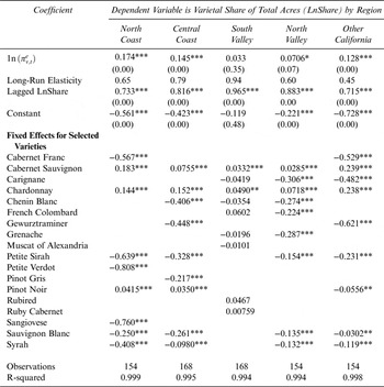
We estimate the model in equation (10) separately for each of the five California regions defined in Table 1 (see online supplementary Appendix Table A-1) using the data for the nineteen years 1995–2013 on the top 12 varieties grown in the region—a total of 228 observations per region if we do not have any missing observations. Hence, a total of 20 different varieties were included for at least one region, reflecting the different varietal emphasis among the regions. In each region the top 12 varieties account for at least 82 percent of total acreage, but not all varieties are grown in all regions, and the shares are very unequal: a few varieties account for most of the planted area in each region, the share of acreage of even the tenth-ranked variety is usually around 1 or 2 percent.Footnote 8 We estimated the regional models using OLS with errors clustered by variety to correct for heterogeneity, given the systematically large differences in varietal shares. The results are summarized in Table 7.
Regression Results, Models of Varietal Shares in California Regions, 1995–2013

Notes: P-values in parentheses. Asterisks denote coefficients that are statistically significantly different from zero at 10% (*), 5% (**) and 1% (***) levels of significance.
The models all fit the data very well, accounting for a very high proportion of the variation in varietal shares in each region, as might be expected in a model that includes the lagged dependent variable and a great many fixed effects (one per variety and one per year in each regional model). Of primary interest is the coefficient on the incentive variable, representing the short-run elasticity of varietal shares with respect to the measure of varietal comparative advantage, an indicator of supply response. In four of the regions the estimate of this short-run elasticity is in the range of 0.08 to 0.17 and statistically significantly different from zero at the 10 percent level or better. The model fits less well overall and the elasticity coefficient is smaller and less statistically significant in the two Central Valley regions, especially in the South Central Valley region. On the whole the models are more satisfactory for the other three, predominantly coastal regions that produce generally higher-quality winegrapes.
Many of the coefficients measuring varietal fixed effects are statistically significant (lower half of Table 7) and mostly they are positive indicating, ceteris paribus, a higher share of that variety relative to the default, Grenache. These coefficients are particularly large and statistically significant, especially in the higher-quality regions, for the premium varieties, Cabernet Sauvignon, Chardonnay, Merlot, Pinot Noir, Zinfandel, Syrah, and to a lesser extent, Sauvignon Blanc, Petite Sirah, and Pinot Gris. Given the logarithmic form, a varietal indicator coefficient of 1.0 implies scaling up the share by a factor of 2.72 (a coefficient of 0.5 implies scaling up the share by a factor of 1.65, and a coefficient of –0.2 implies scaling the share down by a factor of 0.82). These fixed effects account for a significant proportion of the variation in varietal shares, but some still is accounted for by variation in the comparative advantage measure.
Table 7 also reports the long-run elasticities implied by the models for the five regions. The long-run elasticity is inferred by dividing the short-run elasticity by the estimated adjustment coefficient: i.e., β π = α π /λ = α π /(1 − α f ). With the exception of the South Central valley region, for which the point estimate is not statistically significant, the long-run elasticity estimates are all remarkably similar across the regions, in the range of 0.45 to 0.80. These estimates are plausible albeit small, suggestive of quite limited response of the varietal mix to changes in relative returns, even in the long run.
VI. Summary and Implications
The data and analysis here reveal five things about vineyards in the United States. First, even though wine and winegrapes are highly differentiated, and a great many diverse varieties are grown, a comparatively small number of varieties dominate the U.S. picture—in some regions just one or two varieties predominate, with the choice depending on climate and market segment targeted.
Second, broadly speaking, the mix of winegrape varieties in the United States is not very different from that in the rest of the world and, since 2000, it has become even less differentiated. The U.S. mix is now closer to that of France, since France is the closest to the global mix.
Third, U.S. regions vary considerably in the mix of varieties in which they specialize. The U.S. regions mostly have been changing like the national aggregate— each becoming more like France and the world as a whole—but some regions are more distinctive (i.e., New York, Oregon, and the Southern Central Valley), and one region (Oregon) has become more different and more specialized in particular varieties for which it appears to have a comparative advantage.
Fourth, U.S. regions vary considerably in the quality of grapes they produce of a given variety, and region-by-variety interactions have complex influences on the pattern of quality and production.
Fifth, we can account for some of the shifting varietal patterns in the U.S. vineyard and in winegrape production using measures of regional varietal comparative advantage, which reflect changes in both demand and supply and producer responses to them. But a significant share of the variation is not explained by our relatively simple model, in part because it only crudely represents the complexities of winegrape growers' long-run expectations, their intentions, the factors that influence them, and the constraints they face. A more-sophisticated representation of those complexities is not possible at present, however, given limitations on available data and other resources.
Supplementary Material
For supplementary material accompanying this paper visit doi:10.1017/jwe.2015.29.