



1. Introduction
The study of turbulent boundary layers (TBLs) is a fundamental aspect of turbulence research: TBLs enhance momentum and heat transfer rates compared to their laminar counterparts, and play a significant role in determining the aerodynamic performance of aircraft, turbomachines, wind turbines, and underwater vehicles. There has been much work on zero-pressure-gradient (ZPG) TBLs (George & Castillo Reference George and Castillo1997; Smits et al. Reference Smits, McKeon and Marusic2011), reaching a consensus on the scaling of the velocity in the overlap region (Marusic et al. Reference Marusic, Monty, Hultmark and Smits2013):
 \begin{equation} U^+=\frac {1}{\kappa }\ln (y^+)+B\quad\text {for }1\ll y^+, \ y/\delta \ll 1, \end{equation}
where
 $U$
is the mean velocity,
 $y$
is the wall-normal coordinate,
 $\kappa \approx 0.4$
is the von Kármán constant,
 $B\approx 5$
is another constant,
 $\delta$
represents an outer length scale, such as channel half-height, boundary layer height or pipe radius, and the superscript
 $+$
denotes normalisation by the viscous units
 $u_\tau$
and
 $\delta _\nu =\nu /u_\tau$
. Furthermore,
 $u_\tau =\sqrt {\tau _w/\rho }$
is the friction velocity,
 $\nu$
is the kinematic viscosity,
 $\tau _w$
is the wall-shear stress, and
 $\rho \equiv 1$
(unit) is the fluid density. The scaling in (1.1), known as the logarithmic law of the wall, involves only local flow variables, and will be termed ‘velocity scaling in its conventional sense’ in this paper.
The existence of the law of the wall relies on the existence of an inner layer (Pope Reference Pope2000), within which we have
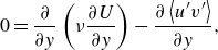 \begin{equation} 0=\frac {\partial }{\partial y}\left (\nu \frac {\partial U}{\partial y}\right )-\frac {\partial \left \lt u^{\prime}v^{\prime}\right \gt }{\partial y}, \end{equation}
where the left-hand side represents the material derivative
 $\textrm { d}U/\textrm { d}t$
and is 0, and the right-hand side contains the viscous stress and the Reynolds stress terms. Here,
 $u^{\prime}$
and
 $v^{\prime}$
are the velocity fluctuation in the streamwise and wall-normal directions, and
 $\left \lt \cdot \right \gt$
denotes an ensemble average. By regarding the Reynolds stress as a ‘stress’ (rather than fluid motion), (1.2) suggests that the net force in the inner region is approximately 0.
The complexity of TBLs increases significantly under the influence of pressure gradients (PGs). PG TBLs are encountered on aircraft wings during takeoff and landing, around the curved surfaces of wind turbine blades, and on the rear sections of underwater vehicles. The presence of a PG can induce flow separation, impacting stability, lift and drag characteristics (Simpson Reference Simpson1989). Such PG TBLs have also been the focus of many works. However, unlike their ZPG counterparts, there is no well-established velocity scaling for PG TBLs.
Before any discussion on the velocity scaling for PG TBLs, a more fundamental question is the existence of a region where a velocity scaling in the conventional sense can exist. As the net force on a fluid parcel is no longer 0 in PG TBLs, Newton’s second law dictates
 \begin{equation} F=ma \end{equation}
and
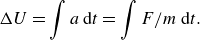 \begin{equation} \Delta U = \int a\,\textrm {d}t = \int F/m \,\textrm {d}t. \end{equation}
Thus fluid velocity or the change therein becomes a cumulative function of the net force over time, rather than being directly correlated to the local force. Here,
 $F$
is the net force on a fluid parcel, including the imposed PG and the viscous and Reynolds stresses,
 $m$
is the mass of the fluid parcel,
 $a$
is the acceleration of the fluid parcel, and
 $t$
is time.
Perry et al. (Reference Perry, Bell and Joubert1966), among others, posited the existence of a region in PG TBLs where the velocity is determined locally. They divided the PG TBL into a ‘wall region’ and a ‘history region’. In the wall region, a velocity scaling in its conventional sense exists. Although the exact mechanism of a wall region is still a research topic, its existence can be argued through the concept of (quasi)-equilibrium boundary layers (EBLs). Kader & Yaglom (Reference Kader and Yaglom1978) argued that a TBL is in equilibrium if the freestream velocity
 $U_\infty$
and the PG
 $P_x$
vary slowly in the flow direction. Townsend and Mellor & Gibson introduced self-similarity of the mean velocity defect as the criterion for equilibrium (Mellor & Gibson Reference Mellor and Gibson1966; Townsend Reference Townsend1976), showing that the flow is at equilibrium if the freestream velocity follows the power law
 $U_\infty = C(x-x_0)^m$
, where
 $C$
is a constant,
 $x_0$
is a virtual origin, and the power law exponent is
 $m\gt -1/3$
. It follows from this definition that some types of favourable PG (FPG) TBLs and mild adverse PG (APG) TBLs are at equilibrium (Skote et al. Reference Skote, Henningson and Henkes1998; Lee & Sung Reference Lee and Sung2009; Lee Reference Lee2017). Evidently, ZPG TBLs are at equilibrium as well (Schlatter et al. Reference Schlatter, Örlü, Li, Brethouwer, Fransson, Johansson, Alfredsson and Henningson2009; Bailey et al. Reference Bailey2013). In these flows, a wall region exists, and the velocity can be expressed using local flow variables.
This study addresses primarily large APGs, and a wall region is not essential. Nonetheless, examining existing literature on the topic will be instructive. Perry et al. (Reference Perry, Bell and Joubert1966), alongside other researchers (Galbraith et al. Reference Galbraith, Sjolander and Head1977; Alving & Fernholz Reference Alving and Fernholz1995; Johnstone et al. Reference Johnstone, Coleman and Spalart2010), have documented the persistence of the logarithmic law of the wall in the wall region, albeit with a diminished logarithmic region compared to ZPG TBLs (Monty et al. Reference Monty, Harun and Marusic2011; Vinuesa et al. Reference Vinuesa, Rozier, Schlatter and Nagib2014). Monkewitz & Nagib (Reference Monkewitz and Nagib2023) and Vishwanathan et al. (Reference Vishwanathan, Fritsch, Lowe and Devenport2023) observed variations in the constants of the logarithmic law as influenced by the PG. Moreover, Monkewitz & Nagib (Reference Monkewitz and Nagib2023), among others (Yang et al. Reference Yang, Sadique, Mittal and Meneveau2015; Luchini Reference Luchini2017; Lv et al. Reference Lv, Huang, Yang and Yang2021), have explored the inclusion of a linear term in the velocity scaling. In addition to the logarithmic law and its variations, some studies have identified a half-power law prevailing above the logarithmic region (Stratford Reference Stratford1959; Perry et al. Reference Perry, Bell and Joubert1966; Kader & Yaglom Reference Kader and Yaglom1978; El Telbany & Reynolds Reference El Telbany and Reynolds1980; Coleman et al. Reference Coleman, Rumsey and Spalart2018). Wei et al. (Reference Wei, Li, Knopp and Vinuesa2023) further established a scaling law for velocity in the wall-normal direction. Efforts to unify velocity scalings across the viscous sublayer, buffer layer, logarithmic layer and square-root layer have also been reported, contributing to a more cohesive understanding of velocity dynamics in TBLs (Materny et al. Reference Materny, Dróżdż, Drobniak and Elsner2008; Dróżdż et al. Reference Dróżdż, Elsner and Drobniak2015; Knopp et al. Reference Knopp, Reuther, Novara, Schanz, Schülein, Schröder and Kähler2021; Knopp Reference Knopp2022; Romero et al. Reference Romero, Zimmerman, Philip, White and Klewicki2022a , Reference Romero, Zimmerman, Philip and Klewickib ; Subrahmanyam et al. Reference Subrahmanyam, Cantwell and Alonso2022).
While (quasi-)equilibrium is not hard to fathom at the limit of ZPG, Bobke et al. (Reference Bobke, Vinuesa, Örlü and Schlatter2017), among others (Vinuesa et al. Reference Vinuesa, Örlü, Sanmiguel Vila, Ianiro, Discetti and Schlatter2017; Parthasarathy & Saxton-Fox Reference Parthasarathy and Saxton-Fox2023), highlighted clear history effects in PG TBLs, even at moderate PGs, challenging the existence of a wall region, and by extension, the existence of any velocity scaling in the conventional sense. For instance, Bobke et al. (Reference Bobke, Vinuesa, Örlü and Schlatter2017) found that the velocity profiles in two TBLs differ due to different histories of the imposed PG even though the Clauser PG parameters and the friction Reynolds numbers match. In light of this significant role of history effects and the complexity of flow history itself, Pozuelo et al. (Reference Pozuelo, Li, Schlatter and Vinuesa2022) proposed to establish a family of baselines for non-equilibrium PG TBLs . They followed Clauser (Reference Clauser1954) and suggested that a good baseline could be PG TBLs where the Clauser PG parameter
 \begin{equation} \beta =\frac {\delta ^* P_x}{\tau _w} \end{equation}
does not change, where
 $\delta ^*$
is the displacement height, and
 $P_x$
is the PG. It is worth noting that velocity profiles in such PG TBLs were termed ‘equilibrium profiles’ by Clauser (Reference Clauser1954), which is a rather odd use of the word ‘equilibrium’. In the same paper, Clauser also defined EBLs as TBLs for which the profiles are identical when
 $(U-U_\infty )/u_\tau$
is plotted against
 $y/\delta$
, which is a more typical use of the word ‘equilibrium’. This paper does not involve or need the concept of equilibrium, but it is still instructive to know that the word has different bearings in different papers and even in the same paper. Reynolds number effect is also critical. The increasing Reynolds number was known to lead to a decreasing APG effect (Sanmiguel Vila et al. Reference Sanmiguel Vila, Örlü, Vinuesa, Schlatter, Ianiro and Discetti2017; Tanarro et al. Reference Tanarro, Vinuesa and Schlatter2020; Pozuelo et al. Reference Pozuelo, Li, Schlatter and Vinuesa2022; Deshpande et al. Reference Deshpande, van den Bogaard, Vinuesa, Lindić and Marusic2023).
Given the difficulty in defining any velocity scaling in the history region, there is limited discussion on the behaviours of the velocity scaling therein. Chen et al. (Reference Chen, Wu, Griffin, Shi and Yang2023a ) seems to be the only work that claimed to have found a velocity scaling in the history region. In that work, the authors proposed a velocity transformation that maps the velocity profiles in the history region back to the logarithmic law of the wall. The transformation contains an integral of the total shear stress, through which it accounts for history effects in the flow. However, since the integral cannot be evaluated locally, the potential utility of the velocity transformation in turbulence modelling is limited.
Based on this literature review, we may conclude the following. The existing literature predominantly focuses on velocity: on the one hand, velocity scaling in the conventional sense can be anticipated in the wall region, although the exact form of the scaling is still a research topic; on the other hand, no velocity scaling in the conventional sense exists in the history region. This study moves away from the conventional velocity analysis to focus on fluid acceleration, i.e.
 $ \bar {{D}}U/\bar {{D}}t$
and its scaling in PG TBLs. In particular, our approach involves making an analogy between the velocity in a ZPG boundary layer and the fluid acceleration in a PG boundary layer.
In preparation for the ensuing discussion, we highlight several key considerations. First, from the standpoint of turbulence modelling, APGs present a more compelling subject of study than FPGs. Perry et al. (Reference Perry, Bell and Joubert1966) noted that the existing wall law is adequate for FPG TBLs. Kays et al. (Reference Kays, Crawford and Weigand1980) demonstrated that models based on a ZPG boundary layer wall law work well under conditions of strong acceleration and very mild deceleration, with discrepancies primarily emerging in scenarios involving APGs – a finding recently reaffirmed by Volino (Reference Volino2020). Spalart & Watmuff (Reference Spalart and Watmuff1993) further articulated the greater practical and theoretical relevance of APGs over FPGs. In alignment with this research trajectory, our study will concentrate on large APGs, where the presence of a wall region is not anticipated. Second, we introduce the laminar Stokes solution (Schlichting & Gersten Reference Schlichting and Gersten2016), which is a very good approximation of the mean flow when a fully developed channel flow is subjected to a suddenly imposed PG, although for a limited time:
 \begin{equation} \frac {{U}}{At}=1+\frac {2}{\sqrt {\pi }}\,\hat {y}\exp(-\hat {y}^2)-(1+2\hat {y}^2)\,\textrm {erfc}(\hat {y}). \end{equation}
Here,
 $A$
is the bulk fluid acceleration,
 $\hat {y}=y/(2\sqrt {\nu t})$
is a self-similarity variable, and
 $\textrm {erfc}(\cdot )$
denotes the complementary error function. Finally, we note that the method of analogy is prevalent in turbulence research, drawing parallels between turbulent phenomena and other more well-understood physical phenomena, both within and beyond the field of turbulence. Examples include: the Reynolds analogy, which relates the turbulent transfer of momentum to the turbulent transfer of heat (So & Speziale Reference So and Speziale1999); Prandtl’s mixing length theory, which attempts to model the turbulent viscosity using an analogy to molecular viscosity (Prandtl Reference Prandtl1925; Bradshaw Reference Bradshaw1974); the Raupach’s mixing layer analogy, which relates the mixing layer and the shear layer formed at the top of surface roughness in rough-wall boundary layers (Raupach et al. Reference Raupach, Finnigan and Brunet1996; Zhang et al. Reference Zhang, Zhu, Yang and Wan2022); and the analogy between the turbulent transient channel flow experiencing a step increase in its Reynolds number and the laminar–turbulent bypass transition (He & Seddighi Reference He and Seddighi2013, Reference He and Seddighi2015). The analogy in He & Seddighi (Reference He and Seddighi2013, Reference He and Seddighi2015) highlights parallels between temporally evolving channel flow and spatially developing boundary layer flow, and as we will see, is particularly relevant to this study. A similar process was found in rapidly accelerating/decelerating turbulent pipe flows (He et al. Reference He, Seddighi and He2016; Guerrero et al. Reference Guerrero, Lambert and Chin2023). Taylor & Seddighi (Reference Taylor and Seddighi2024) extended the analogy in He & Seddighi (Reference He and Seddighi2015) to the turbulent channel with intermediate- and low-frequency pulsations.
The rest of the paper is organised as follows. The model problem is described in § 2. Details of the log-layer analogy are presented in § 3, with validation results in § 4. Finally, concluding remarks are given in § 5.
2. Model problem
Consider the scenario of a spatially developing TBL influenced by PGs. The complexity arises from the turbulent nature of the flow and from the potentially complex patterns of the PG force, which may be represented as
 \begin{equation} P_x=P_0+\sum _{i} P_i\cos (k_ix+\phi _i), \end{equation}
where
 $P_x$
is the PG force,
 $P_i$
is the amplitude,
 $k_i$
is the wavenumber,
 $x$
is the streamwise coordinate, and
 $\phi _i$
is a phase. Analysing the interplay among the many scales that make up the PG and the many scales in a boundary layer presents a considerable challenge – and is unnecessary. Here, we limit ourselves to a constant PG
 \begin{equation} P_x=P_0. \end{equation}
The model flow problem is illustrated in figure 1(a), depicting an initial EBL subjected to an APG. This leads to the development of an internal boundary layer (IBL) (Smits & Wood Reference Smits and Wood1985; Baskaran et al. Reference Baskaran, Smits and Joubert1987; Garratt Reference Garratt1990; Li et al. Reference Li, de Silva, Chung, Pullin, Marusic and Hutchins2022). The IBL is initially laminar, and its behaviour can be described by the Stokes solution. It then undergoes a transition before becoming turbulent downstream, where flow separation may occur.
Schematic of the model problem: (a) the spatially developing boundary layer (BL) flow subjected to an APG; (b) the temporally evolving channel flow with an APG. The IBL is initially laminar, then transitions to turbulence, and may eventually separate.
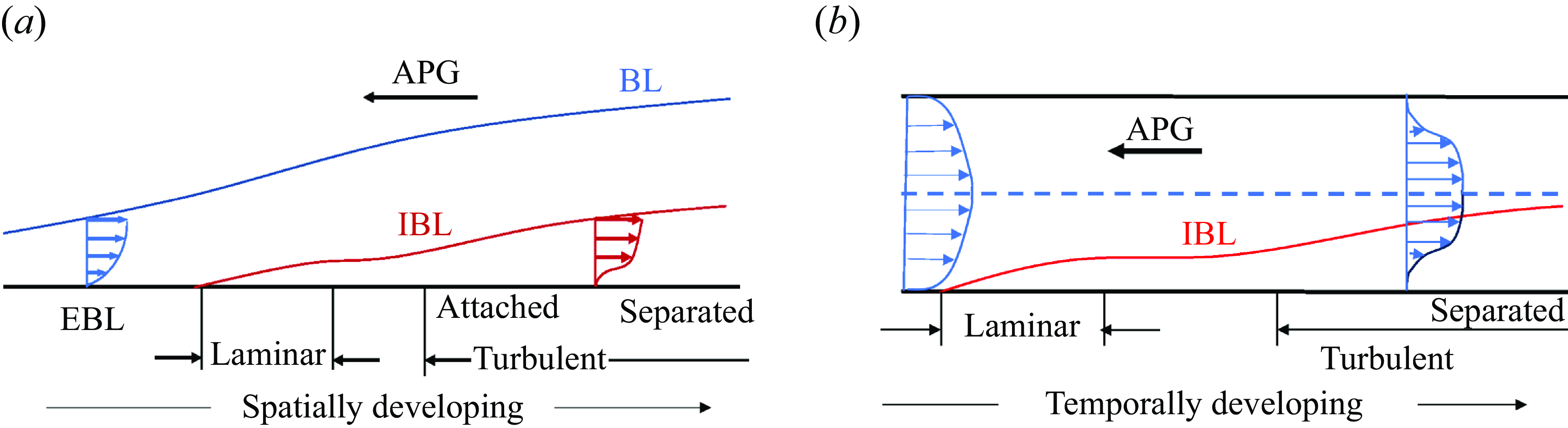
The discussion thus far has centred on spatially developing boundary layers; however, the principles discussed are equally applicable to temporally evolving boundary layers. Temporal simulations, particularly of wakes and mixing layers – which are traditionally conceptualised as spatially developing phenomena – have demonstrated considerable effectiveness (Brucker & Sarkar Reference Brucker and Sarkar2010; de Stadler et al. Reference de Bruyn Kops and Riley2010; de Bruyn Kops & Riley Reference de Bruyn Kops and Riley2019; Li et al. Reference Li, Yang and Kunz2024). Particularly relevant to this study is the exploration of temporal simulations as alternatives to spatially developing ZPG TBLs in Kozul et al. (Reference Kozul, Chung and Monty2016). Additionally, temporal simulations of PG TBLs have been reported, notably in studies by He & Seddighi (Reference He and Seddighi2015), Mathur et al. (Reference Mathur, Gorji, He, Seddighi, Vardy, O’Donoghue and Pokrajac2018) and Lozano-Durán et al. (Reference Lozano-Durán, Giometto, Park and Moin2020), where a common focus is on the dynamics of a fully developed channel flow when subjected to a suddenly imposed PG. In the context of temporal PG TBLs, as illustrated in figure 1(b), the representation of the PG force adapts to incorporate time, leading to
 \begin{equation} P_x=P_0+\sum _{i} P_i\cos (f_it+\phi _i^{\prime}),\quad P_x=P_0 \end{equation}
instead of (2.1) and (2.2). Here,
 $f_i$
is the frequency.
Comparing a PG TBL and an accelerating or decelerating channel, the most notable difference lies in the outer length scale. In a PG TBL, the outer length scale evolves with the flow, whereas in a channel, it remains fixed at the channel half-height. This difference becomes more pronounced when the flow encounters an APG. The PG induces a negative
 $\partial U/\partial x$
, and due to continuity, a positive
 $\partial V/\partial y$
. The resulting increase in wall-normal velocity thickens the boundary layer, producing a ‘straining effect’ in the outer layer (Coleman et al. Reference Coleman, Kim and Spalart2000, Reference Coleman, Kim and Spalart2003). However, the thickening of the boundary layer has minimal influence on the properties of the inner layer, as the inner layer, by definition, is independent of the outer scale. Consequently, an analogy can be drawn between the inner layer of the spatially developing boundary layer and that of the temporally developing boundary layer. The focus on the inner layer here is motivated by the emerging paradigm of computational fluid dynamics for fluids engineering, where turbulence in the outer layer is resolved directly, and the flow in the wall layer is modelled – often via some sort of mean flow scaling (Bose & Park Reference Bose and Park2018).
3. Theory
In this section, we present the analogy between the velocity in a ZPG TBL and the flow acceleration in a PG TBL.
3.1. The log-layer analogy
We begin by examining the mean flow equation
 \begin{equation} \frac {\bar {D} U}{\bar {D}t}=-P_x+\nu \frac {\partial ^2U}{\partial y^2}-\frac {\partial \left \lt u^{\prime}v^{\prime}\right \gt }{\partial y}. \end{equation}
Here,
 $\bar{D}/\bar {D}t=\partial /\partial t + U\,\partial /\partial x+V\,\partial /\partial y$
is the mean substantial derivative (Pope Reference Pope2000). In the absence of any PG force, the equation above becomes
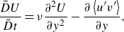 \begin{equation} \frac {\bar {D} U}{\bar {D}t}=\nu \frac {\partial ^2U}{\partial y^2}-\frac {\partial \left \lt u^{\prime}v^{\prime}\right \gt }{\partial y}, \end{equation}
and it describes the development of a ZPG boundary layer. Define fluid acceleration
 \begin{equation} g=\frac {1}{A}\frac {\bar {D} U}{\bar {D}t}, \end{equation}
where
 $A$
is the acceleration outside the IBL. Notice that
 $g$
has no dimension. In this study, we focus on a temporally evolving TBL, therefore
 $g$
becomes
 $(\partial U/\partial t)/A$
. By differentiating (3.1) with respect to time, we derive the governing equation for
 $g$
:
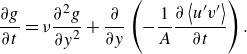 \begin{equation} \frac {\partial g}{\partial t}=\nu \frac {\partial ^2 g}{\partial y^2}+\frac {\partial }{\partial y}\left (-\frac {1}{A}\frac {\partial \left \lt u^{\prime}v^{\prime}\right \gt }{\partial t}\right ). \end{equation}
The PG emerges as a critical flow parameter. Define
 \begin{equation} \zeta = -A\nu \big/(\tau _{w,0}/\rho )^{3/2}. \end{equation}
This parameter is analogous to the Clauser PG parameter (Clauser Reference Clauser1956), but instead of the displacement height, we employ the viscous length scale for non-dimensionalisation.
We see that (3.2) and (3.4) have similar forms, suggesting an analogy between the velocity
 $U$
in a ZPG TBL and the fluid acceleration
 $g$
in PG TBLs. In particular, since
 \begin{equation} U=f_1\left (\nu , \left .\nu \frac {\partial U}{\partial y}\right |_{w},y\right )\quad\text {for}\ y\ll \delta , \end{equation}
in a ZPG TBL, by the analogy, we should have
 \begin{equation} g=f_2\left (\nu , \left .\nu \frac {\partial g}{\partial y}\right |_{w},y\right )\quad\text {for}\ y\ll \delta , \end{equation}
in a PG TBL. Here,
 $f_1$
and
 $f_2$
are generic functions, and the subscript
 $w$
denotes quantities evaluated at the wall. Applying dimensional analysis to (3.6) gives
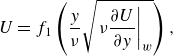 \begin{equation} U=f_1\left (\frac {y }{\nu }\sqrt {\left .\nu \frac {\partial U}{\partial y}\right |_{w}}\right ), \end{equation}
in a ZPG TBL, and similarly,
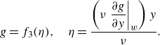 \begin{equation} g=f_3(\eta), \quad \eta =\frac {\left (\nu \left .\dfrac {\partial g}{\partial y}\right |_w\right )y}{\nu }. \end{equation}
Before we proceed further, we study the limit of
 $P_x$
approaching 0, i.e. the ZPG TBL, a limit that is fairly well understood. A direct consequence of (3.3), (3.5) and (3.9) is
 \begin{equation} \frac {\bar {D}U^+}{\bar {D}t^+}=\zeta\, f_3(\eta )=\frac {-A \delta }{u_\tau ^2}\,\frac {f_3(\eta )}{Re_\tau }. \end{equation}
where
 $Re_\tau=u_\tau \delta/\nu$
is the friction Reynolds number. When
 $P_x=0$
,
 $A=-u_\tau ^2/\delta$
and
 $\bar {D}U^+/\bar {D}t^+\sim 1/Re_\tau$
, which is consistent with the result in Morrill-Winter et al. (Reference Morrill-Winter, Philip and Klewicki2017).
3.2.
Scaling of the acceleration
 $g$
and the velocity
$U$


We now examine (3.9). It is easy to verify that (3.9) is consistent with the Stokes solution (1.6):
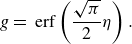 \begin{equation} g = \textrm { erf}\left (\frac {\sqrt {\pi }}{2}\eta \right ). \end{equation}
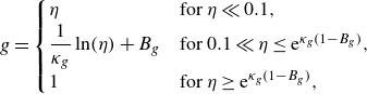
The Stokes solution is valid when the IBL is laminar. When the IBL becomes turbulent, we anticipate the scaling
 \begin{equation}g=\begin{cases} \eta &\text {for}\ \eta \ll 0.1,\\ \dfrac {1}{\kappa _g}\ln (\eta)+B_g &\text {for}\ 0.1 \ll \eta \le {\rm e}^{\kappa _g(1-B_g)},\\ 1 &\text {for}\ \eta \ge {\rm e}^{\kappa _g(1-B_g)}, \end{cases}\end{equation}
mirroring the mean velocity
 $U$
in a ZPG TBL. The first line in this equation is the scaling in the sublayer, which can be confirmed directly by evaluating (3.4) at the wall as follows. Because
 $g=0$
at the wall,
 $\partial g/\partial t=0$
. Also, because
 $\left \lt u^{\prime}v^{\prime}\right \gt =O(y^3)$
,
 $\partial ^2 \left \lt u^{\prime}v^{\prime}\right \gt /\partial y\,\partial t=0$
at the wall. Consequently, (3.4) simplifies to
 \begin{equation} \left .\nu \frac {\partial ^2 g}{\partial y^2}\right |_w=0 \end{equation}
at the wall, leading directly to the sublayer scaling
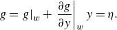 \begin{equation} g=\left .g\right |_w+\left .\frac {\partial g}{\partial y}\right |_w y=\eta . \end{equation}
The second line in (3.12) is the scaling of
 $g$
in the inertial layer. The two constants
 $\kappa _g$
and
 $B_g$
are analogous to the two constants
 $\kappa$
and
 $B$
in the law of the wall, albeit without implying their universality. The selection of
 $\eta =0.1$
as a threshold between linear and logarithmic scaling is based on the rationale that the viscous sublayer should be unaffected by freestream conditions, necessitating
 $g\ll 1$
in the sublayer. With the choice
 $g\ll 0.1$
, we have
 $\eta =g\ll 0.1$
in the sublayer. The exact location of transition between the linear and logarithmic scalings depends on the balance between the two terms in (3.4). When the bulk flow acceleration is dominant, the transition from the linear scaling to the viscous scaling occurs at a large
 $\eta$
; conversely, when the turbulent term is dominant, the transition occurs at a small
 $\eta$
– which we will verify against empirical data in § 4.2. Finally, the last line in (3.12) represents the transition from the IBL to the outside boundary layer, where the acceleration is constant. The transition location is determined by assuming that
 $g$
is monotonically increasing.
The scalings of the fluid acceleration in (3.12) have implications for the scaling of the velocity. Integrating
 $g$
, we should have
 \begin{equation} \begin{aligned} U(y,t)=U(y,t_2)+\int _{t_2}^{t} A\, g(\eta (y,t))\, {\rm d}t, \end{aligned} \end{equation}
where
 $t_2$
marks the time when the IBL becomes turbulent.
4. Validation
4.1. Validation data
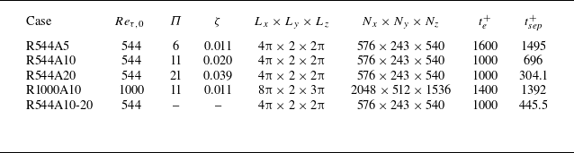
We focus on temporally evolving TBLs, employing direct numerical simulations (DNS) to examine a fully developed turbulent channel flow subjected to a suddenly imposed APG. The flow is transient and is controlled by the Reynolds number, i.e.
 $Re_{\tau ,0}=\delta u_{\tau ,0}/\nu$
, and the magnitude of the APG (on top of the PG that drives the initial flow), i.e.
 $\Pi =P_x \delta /\tau _{w,0}+1$
. Here,
 $\delta$
is the channel half-height, and the subscript 0 denotes the state before the PG is applied. Table 1 tabulates the details of our DNS, including
 $Re_{\tau ,0}$
,
 $\Pi$
,
 $\zeta$
, the simulation time, and the time it takes for incipient separation. The bulk flow acceleration is
 $A=-(P_x+\tau _{w,0})/(\rho \delta )$
, and
 $\zeta =\Pi /Re_{\tau ,0}$
. Notice that
 $\zeta \sim Re_\tau ^{-1}$
for a given PG, implying that the effects of PGs decrease with the Reynolds number (Tanarro et al. Reference Tanarro, Vinuesa and Schlatter2020; Deshpande et al. Reference Deshpande, van den Bogaard, Vinuesa, Lindić and Marusic2023). We explore two distinct Reynolds numbers,
 $Re_{\tau ,0}=544$
and 1000, across a range of PG forces, with
 $\Pi$
values extending from 5 to 20. The flow maintains homogeneity in both the streamwise and spanwise directions, allowing for averages to be taken across these axes. Additionally, ensemble averages are computed from eight independent realisations to ensure statistical convergence. The numerics of our DNS code are identical to those in Lee & Moser (Reference Lee and Moser2015). Further details of the code can be found in Chen et al. (Reference Chen, Zhu, Shi and Yang2023b
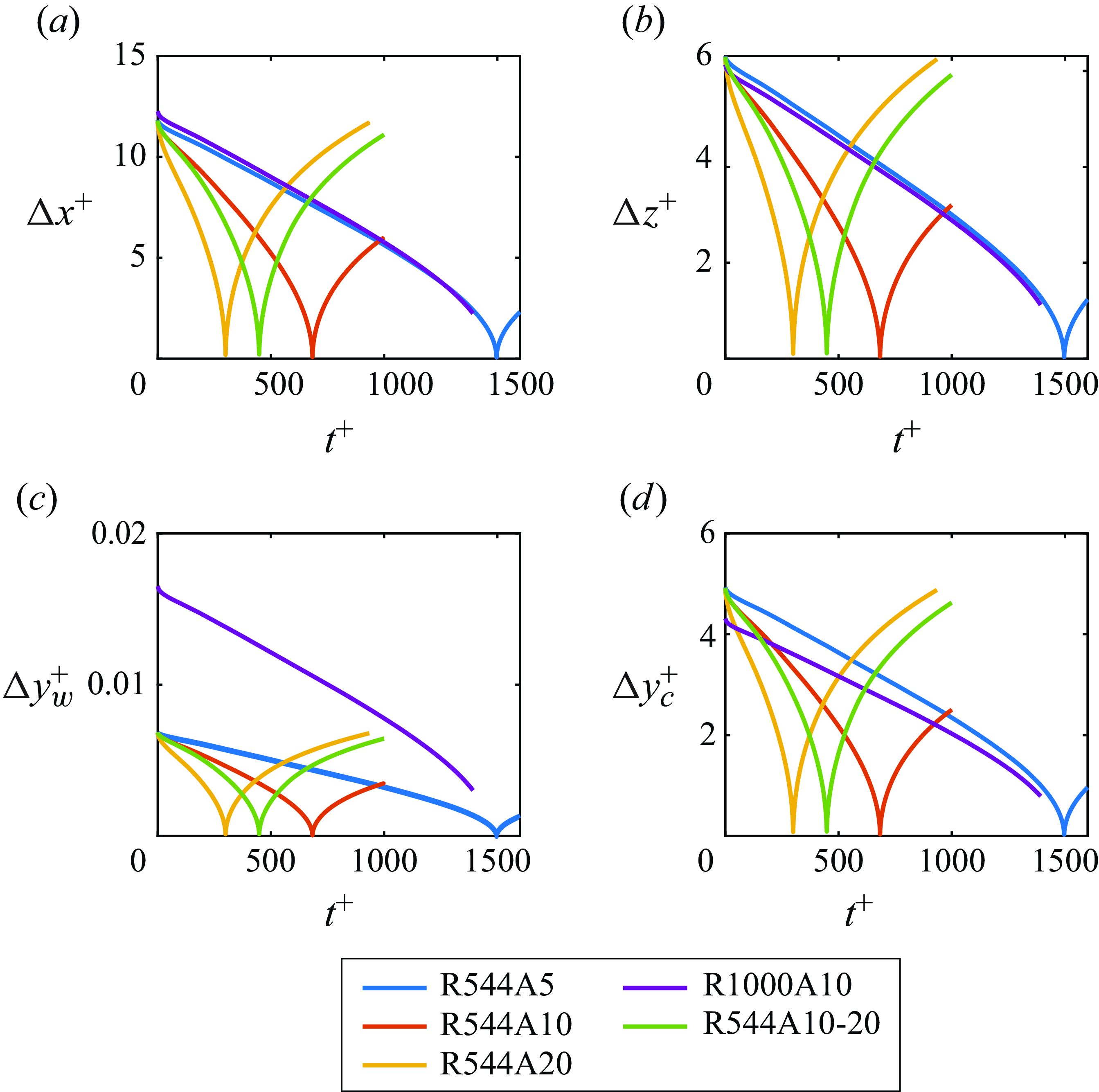
) and Graham et al. (Reference Graham2016), and are not repeated here for brevity. The domain sizes are listed in table 1, which are larger than the minimal channel in Lozano-Durán & Jiménez (Reference Lozano-Durán and Jiménez2014). Figure 2 illustrates the grid resolutions as the flow evolves, normalised using the instantaneous friction scales. The flow initially decelerates, then accelerates in the opposite direction. Throughout the entire evolution process, the grid resolutions adhere to established heuristics:
 $\Delta x^+ \lesssim 10$
,
 $\Delta z^+ \lesssim 6$
,
 $\Delta y_w^+ \lt 1$
and
 $\Delta y_c^+ \lesssim 6$
(Kim et al. Reference Kim, Moin and Moser1987; Chen et al. Reference Chen, Zhu, Shi and Yang2023b
).
Details of the DNS. The nomenclature is R[
 $Re_{\tau ,0}$
]A[
 $P_x/\tau _{w,0}$
]. We list the initial Reynolds number
 $Re_{\tau ,0}=\delta u_{\tau ,0}/\nu$
, the PG
 $\Pi =P_x\delta /\tau _{w,0}+1$
, the non-dimensional PG
 $\zeta =-A\nu /u_{\tau ,0}^3$
, the size of the computational domain
 $L_x$
,
 $L_y$
and
 $L_z$
, the grid size
 $N_x$
,
 $N_y$
and
 $N_z$
, and the simulation time
 $t_e$
and the time until incipient separation
 $t_{sep}$
. The superscript
 $+$
indicates normalisation by
 $\nu /u_{\tau ,0}^2$
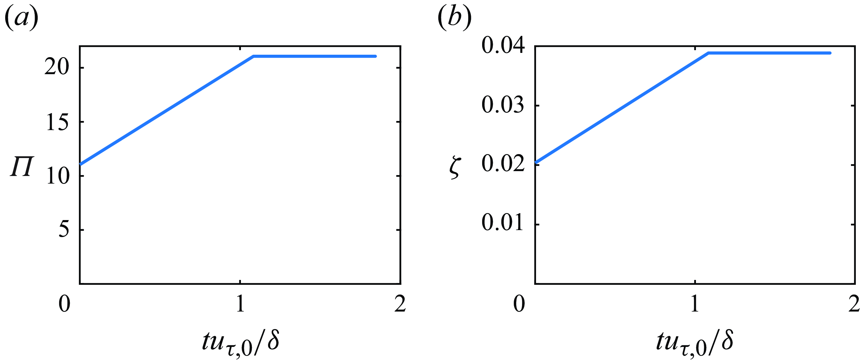
. For R544A10-20,
 $\Pi$
and
 $\zeta$
vary, and their variations are illustrated in figure 3.
Grid resolution normalised with the instantaneous friction scales, i.e.
 $\delta _\nu (t)=\nu /\sqrt {|\tau _w|/\rho }$
. Here,
 $\Delta x$
and
 $\Delta z$
are the grid spacings in the streamwise and spanwise directions, respectively;
 $\Delta y_w$
is the grid spacing in the wall-normal direction at the wall, and
 $\Delta y_c$
is the one at the centreline.
(a) The PG force
 $\Pi =P_x\delta /\tau _{w,0}$
+1 and (b) the non-dimensional PG parameter
 $\zeta =-A\nu /u_{\tau ,0}^3$
, as functions of
 $tu_{\tau ,0}/\delta$
in R544A10-20.
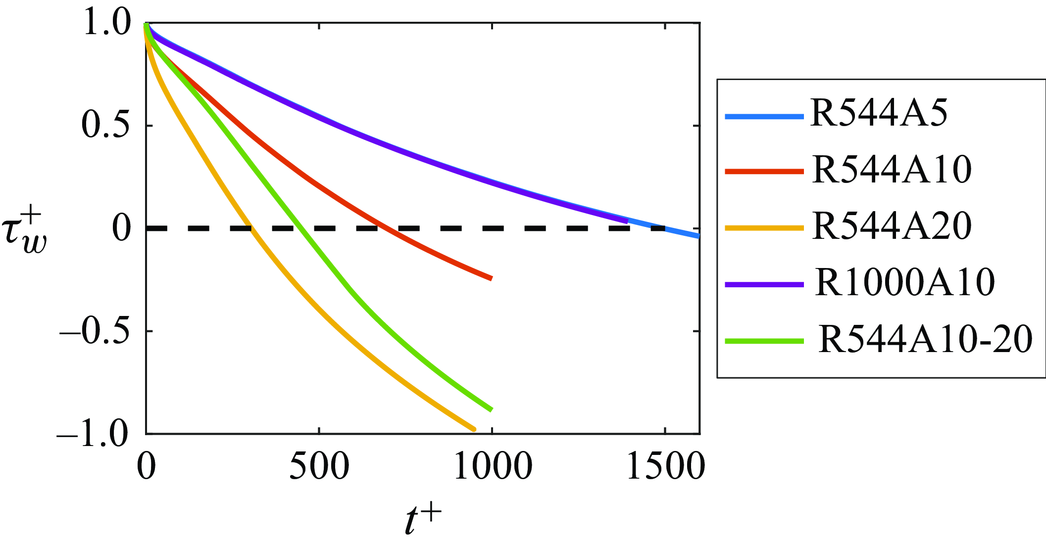
The DNS are not the focus of the study, and here we show some relevant results. Figure 4 shows the evolution of the wall-shear stress
 $\tau _w$
. The times for incipient separation are listed in table 2. The flow separates earlier when a larger non-dimensional PG is applied. Notice that the R544A5 and R1000A10 results collapse in figure 4, showing the power of
 $\zeta$
as a controlling parameter.
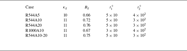
The measured
 $\kappa _g$
and
 $B_g$
. The IBL is laminar for
 $0\lt t\lt t_1$
, and turbulent for
 $t_2\lt t$
.
Evolution of the wall-shear stress in our DNS.
4.2. Validation results
The study has so far corroborated the analogy within the viscous sublayer through comparisons with the Stokes solution and an evaluation of the Navier–Stokes equations at the wall. Nonetheless, the validity (and the usefulness) of any analogy hinges on its validation against empirical data. To this end, we juxtapose (3.11) and (3.12) against experimental and DNS data. Here, (3.11) is equivalent to the Stokes solution and applies to laminar IBLs, i.e.
 $t\lt t_1$
; (3.12) and (3.15), on the other hand, apply to turbulent IBLs, i.e.
 $t\gt t_2$
. Table 2 lists the values of
 $t_1$
and
 $t_2$
for all DNS cases.
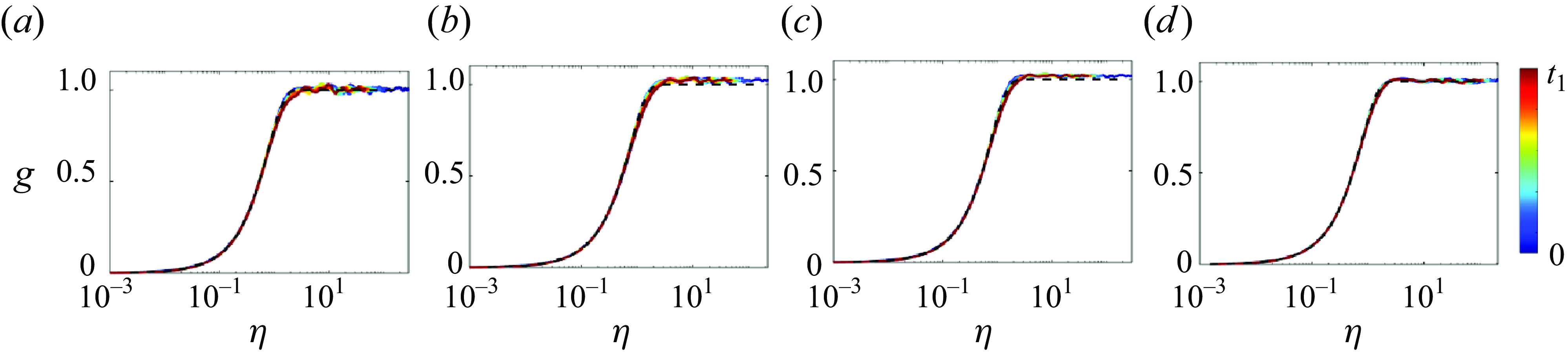
Figure 5 illustrates the flow acceleration
 $g$
as a function of the non-dimensional distance from the wall
 $\eta$
for
 $t\lt t_1$
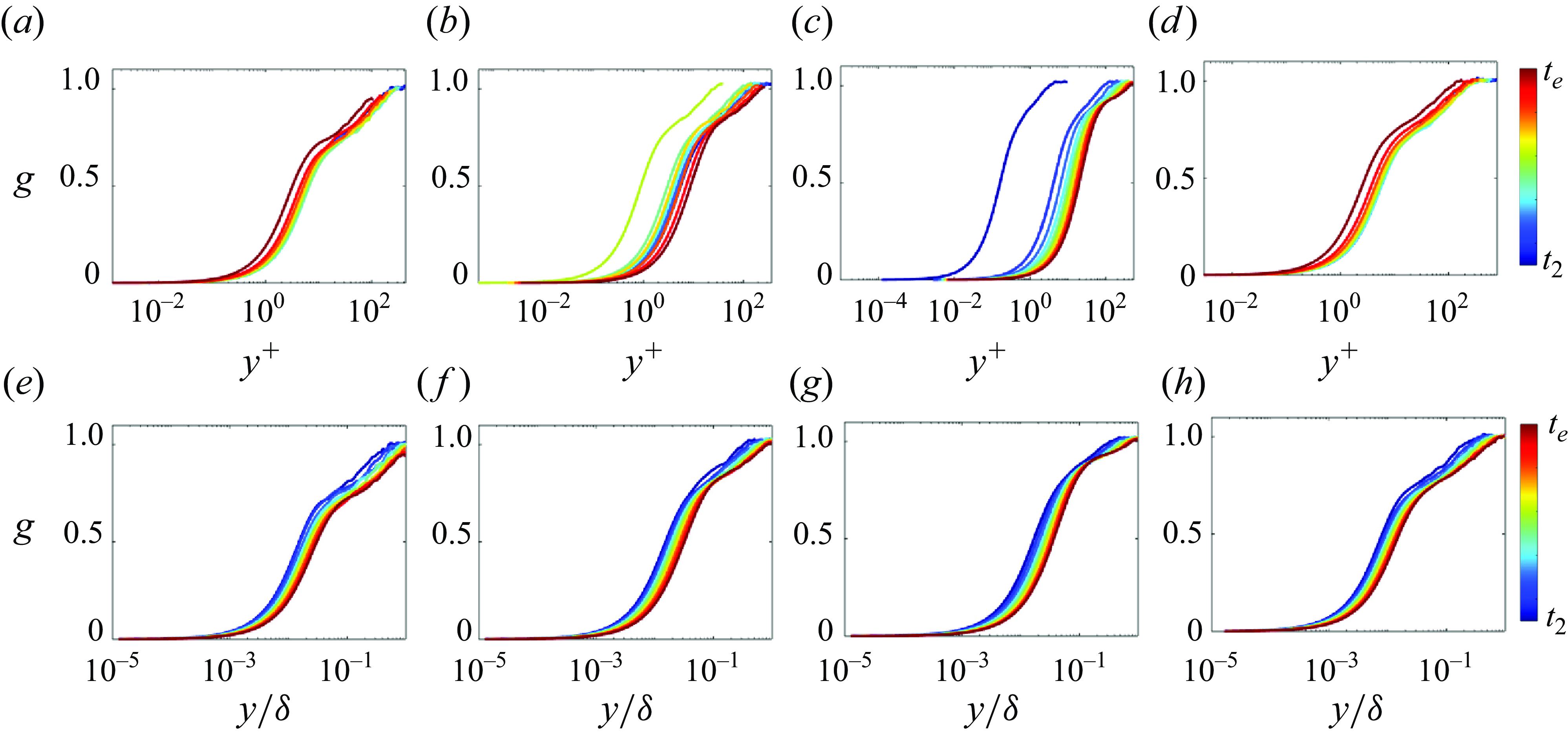
. The data closely follow (3.11). This is not unexpected as the validity of the Stokes solution for laminar IBLs is known. Next, we assess (3.12). We first present profiles of non-dimensional fluid acceleration
 $g$
as a function of conventional wall-normal coordinates
 $y^+$
and
 $y/\delta$
in figure 6. Note that
 $g$
does not collapse when plotted against either
 $y^+$
or
 $y/\delta$
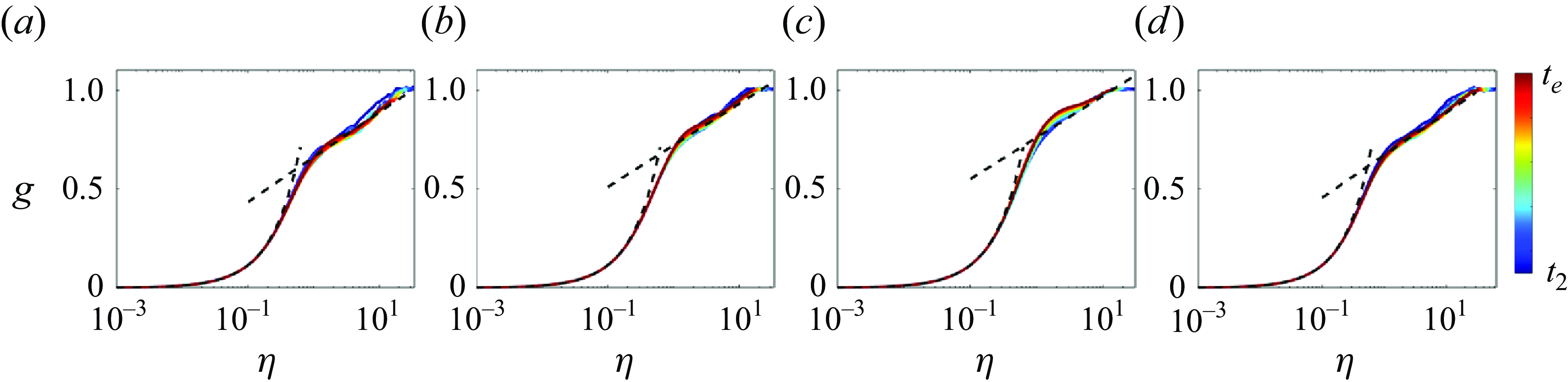
. Figure 7 shows
 $g$
as a function of
 $\eta$
, and we see a good collapse of the profiles. In particular,
 $g$
adheres to a linear scaling in the wall layer and a logarithmic one above, in accordance with (3.12). Furthermore, we see that the transition between the linear and logarithmic scalings moves away from the wall as the non-dimensional PG parameter
 $\zeta$
increases, corroborating the discussion in § 3.
The non-dimensional fluid acceleration
 $g$
as a function of
 $\eta$
for
 $t\lt t_1$
. The profiles are evenly sampled between
 $t=0$
and
 $t=t_1$
: (a) R544A5, (b) R544A10, (c) R544A20, (d) R1000A10. The black dashed line corresponds to (3.11).
The fluid acceleration
 $g$
as a function of (a,b,c,d)
 $y^+$
and (e,f,g,h)
 $y/\delta$
, for (a,e) R544A5, (b,f) R544A10, (c,g) R544A20, (d,h) R1000A10. The profiles are evenly sampled between
 $t=t_2$
and
 $t=t_e$
.
The fluid acceleration
 $g$
as a function of
 $\eta$
: (a) R544A5, (b) R445A10, (c) R544A20, (d) R1000A10. The black dashed lines correspond to the linear and the logarithmic scalings in (3.12). The profiles are evenly sampled between
 $t=t_2$
and
 $t=t_e$
.
The logarithmic scaling in (3.12) contains two parameters,
 $\kappa _g$
and
 $B_g$
, and it is instructive to determine their values. Table 2 lists the measured values of
 $\kappa _g$
and
 $B_g$
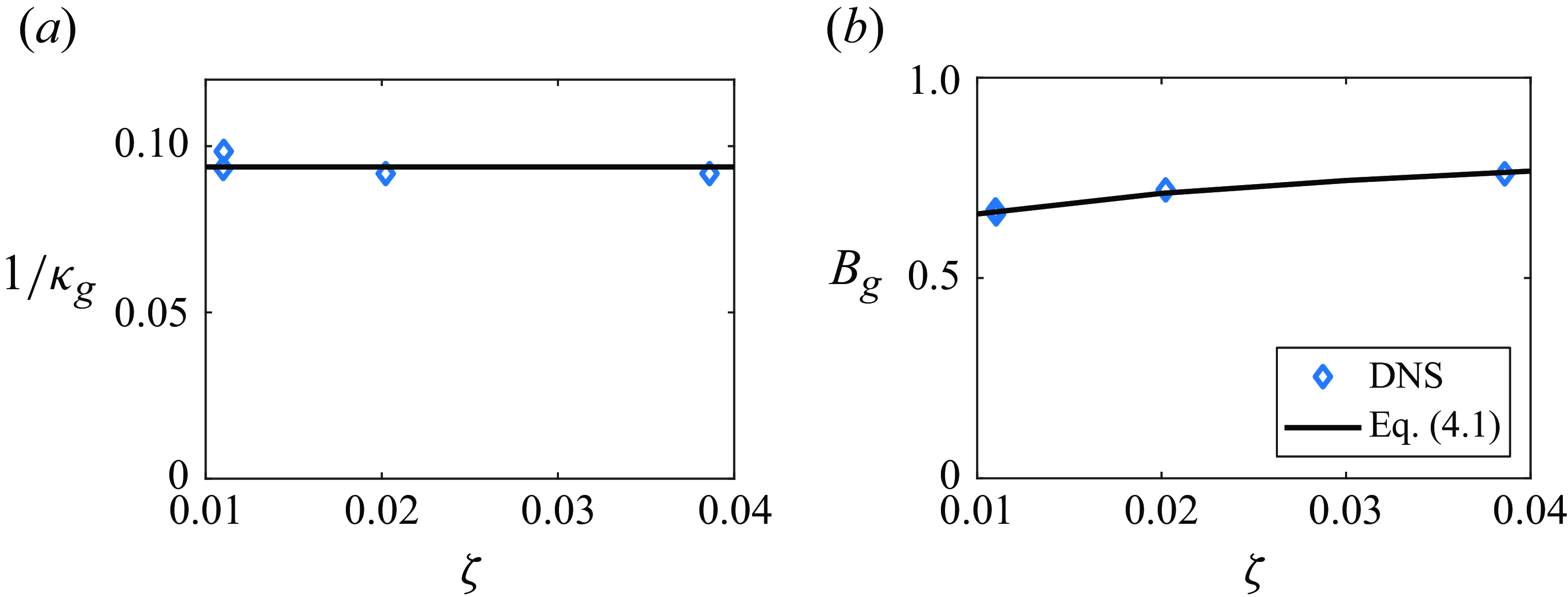
. Figure 8 illustrates
 $\kappa _g$
and
 $B_g$
as functions of the non-dimensional PG parameter
 $\zeta$
. The data indicate that
 $\kappa _g$
is insensitive to the flow condition, and its value is given by
 $1/\kappa _g\approx 0.094\pm 0.004$
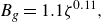
. On the other hand,
 $B_g$
increases slightly as a function of the non-dimensional PG parameter
 $\zeta$
. Its value is 0.66 when
 $\zeta =0.011$
, and 0.8 when
 $\zeta =0.038$
. The present data suggest
 \begin{equation} B_g=1.1 \zeta ^{0.11}, \end{equation}
indicating a weak dependence on
 $\zeta$
.
Plots of (a)
 $1/\kappa _g$
as a function of
 $\zeta$
, and(b)
 $B_g$
as a function of
 $\zeta$
. In (a), the black solid lines represent the mean values of the four cases.
We proceed to examine the effectiveness of the velocity scaling (3.15). Figure 9 compares (3.15) to the DNS data at a few time instants between
 $t=t_2$
and
 $t=t_e$
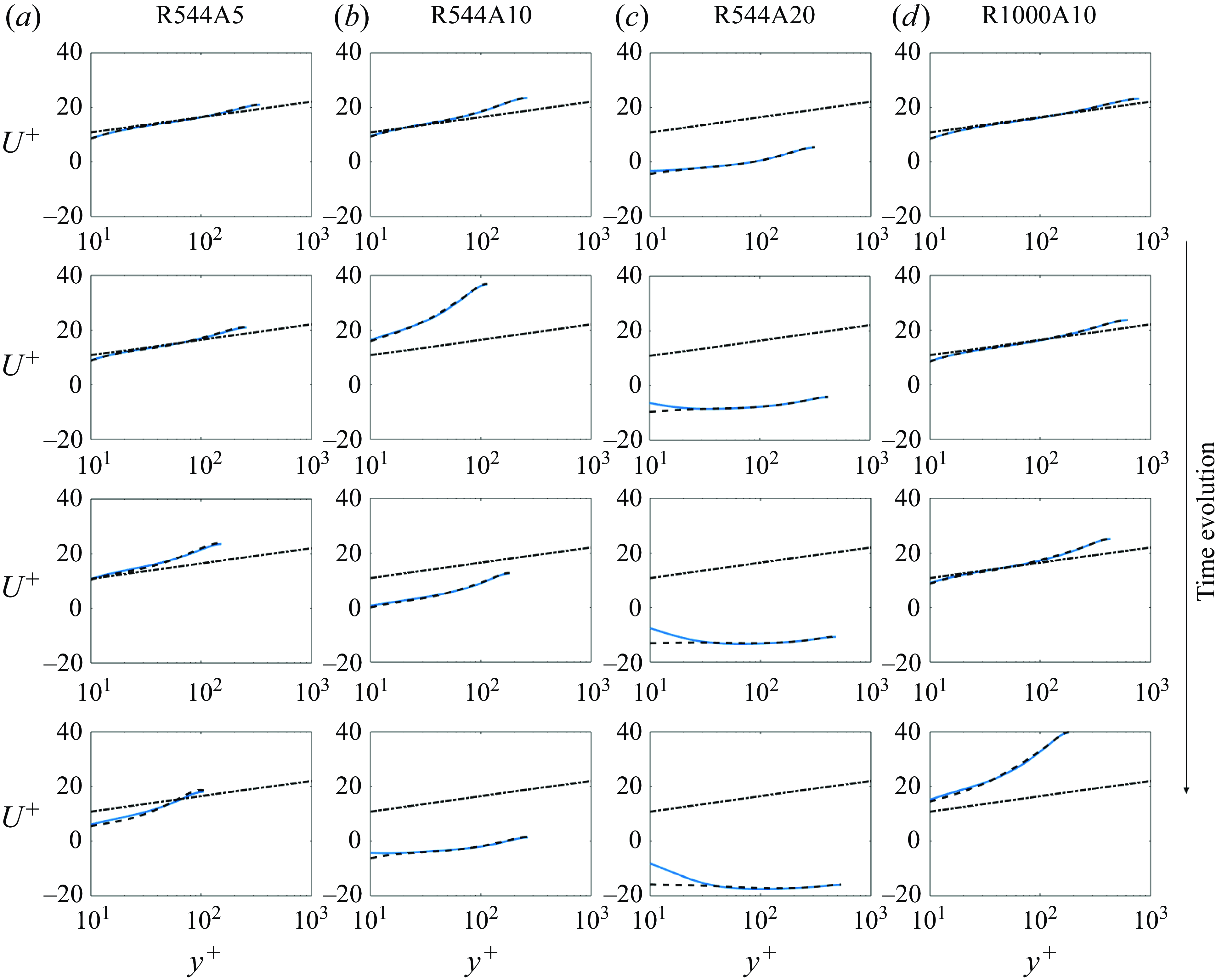
. For comparison purposes, we have also plotted the canonical logarithmic law in (1.1), which proves to be a good approximation of the mean flow for the early times and under conditions of mild APGs. Errors emerge as the flow evolves in R544A10, and particularly in R544A20. In the latter, intense flow deceleration results in flow separation. Consequently, the flow in the wall layer reverses, and is responsible for the significant errors in the canonical logarithmic law. The scaling in (3.15), on the other hand, is accurate across the board, including that leading to flow separation.
Velocity
 $U^+$
as a function of
 $y^+$
at a few time instants between
 $t=t_2$
and
 $t=t_e$
: (a) R544A5, (b) R544A10, (c) R544A20, (d) R1000A10. The dashed lines and the dot-dashed lines correspond to the reference scalings in (3.15) and the canonical law of the wall.
For completeness, we show
 $g$
as a function of
 $\eta$
for
 $t_1\lt t\lt t_2$
in figure 10. The Stokes solution and the logarithmic scaling in (3.12) are plotted for reference purposes. Here, we see that the flow acceleration
 $g$
converges from the Stokes solution to the logarithmic scaling.


4.3. Varying PGs
The analogy is formally developed for constant PGs, and its validity is likewise so restricted. In this subsection, we study the behaviours of fluid acceleration in a TBL with slowly varying PGs, i.e. case R544A10-20, and test if the analogy extrapolates to cases with a varying PG. Like the other cases in table 1, the flow in R544A10-20 is a fully developed channel flow at
 $t=0$
. The following APG is then imposed:
 \begin{equation} \Pi =\begin{cases} 11+10 t u_{\tau ,0}/\delta & \text {for}\ t\lt \delta /u_{\tau ,0},\\ 21 & \text {for}\ t\gt \delta /u_{\tau ,0}.\end{cases} \end{equation}
Notice that the PG doubles over one large-eddy turnover time. We proceed to compare the scalings in (3.11) and (3.12) to data. Figure 11 shows the flow acceleration
 $g$
as a function of
 $\eta$
for
 $t\lt t_1$
,
 $t_1\lt t\lt t_2$
and
 $t_2\lt t$
, i.e. when the IBL is laminar, transitional and turbulent. The data follow the laminar Stokes solution when the IBL is laminar, and the DNS data converge to the scaling in (3.12) as the IBL transitions to turbulence. In particular, we see from figure 11(c) a logarithmic region in the fluid acceleration. The values of the two constants are
 $\kappa _g=10.90$
and
 $B_g=0.75$
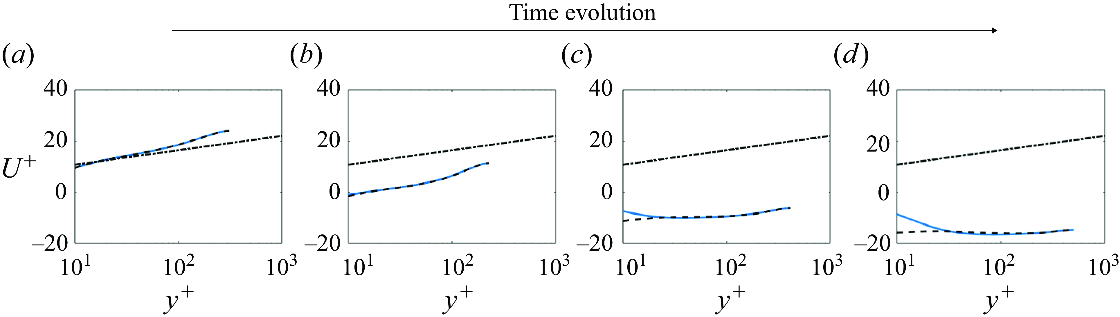
, which are not far from the values in cases R544A10 and R544A20. We further compare the velocity scaling in (3.15) to data; figure 12 shows the results. The canonical law of the wall is included for comparison purposes. The result is similar to that in § 4.2: the canonical log law is accurate initially, but becomes increasingly inaccurate as the flow evolves, whereas the scaling in (3.15) remains accurate. Hence we conclude that the log-layer analogy developed here is applicable to TBLs with slowly varying PGs.


The non-dimensional velocity
 $U^+$
as a function of
 $y^+$
at a few time instants between
 $t=t_2$
and
 $t=t_e$
, for R544A10-20. The dashed lines and dot-dashed lines correspond to the reference scalings in (3.15) and the canonical law of the wall.
5. Conclusions
In the current study, we establish an analogy between the inner layer of equilibrium spatially evolving boundary layers and that of temporally evolving boundary layers with pressure gradients (PGs) by drawing parallels between their governing transport equations. Specifically, we compare the transport equation for velocity in the spatially evolving case with the transport equation for fluid acceleration in the temporally evolving scenario. As previous work has focused on velocity analysis, this study provides a new perspective. Exploiting the log-layer analogy, we drew the following conclusions. First, the fluid acceleration is a function of
 $\eta =(\nu\, \partial g/\partial y)_w\, y/\nu$
in (3.9). Second, analogous to the logarithmic law for velocity, fluid acceleration should exhibit similar scaling behaviours in turbulent IBLs (3.12). Since the integration of acceleration leads to the velocity scaling (3.15), the scaling of the fluid acceleration has implications for the velocity scaling. Third, the non-dimensionalised PG force
 $\zeta =-A\nu \big /(\tau _{w,0}/\rho )^{3/2}$
emerges as an important parameter, suggesting that flows with similar
 $\zeta$
values exhibit similar behaviours. Empirical validation of this analogy was pursued through comparisons with the Stokes solution for laminar flows immediately after the application of a PG, and through direct numerical simulations of fully developed channel flows under suddenly imposed adverse PGs. These comparisons yielded highly favourable outcomes, supporting the analogy’s applicability. Nonetheless, by focusing on the channel configuration and maintaining the channel half-height, the present work neglects the impacts of varying outer length scales. Therefore, its applicability to boundary layer flows is yet to be tested, a topic left for future investigation.
Funding.
We acknowledge the support from NSFC (grant nos 11988102, 12102168, 12225204), Shenzhen Science & Technology Program (grant no. KQTD20180411143441009), Department of Science and Technology of Guangdong Province (grant nos 2023B1212060001, 2020B1212030001). X.I.A.Y. acknowledges Office of Naval Research, grant no. N000142012315.
Declaration of interests.
The authors report no conflict of interest.
Data availability statement.
The data that support the findings of this study are available from the corresponding author upon reasonable request.



