2.1. General setting

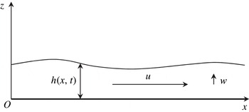
Consider the Euler equations for two-dimensional flows over a flat bottom. The choice of such a simplified topography allows us to separate the study of wave–shear current interaction and geometrical effects due to the bottom topography that naturally induce vertical flows. The introduction of the bottom topography, which is important for applications, can be given in a standard way. In Cartesian coordinate system $Oxz$ , the horizontal velocity component in direction $Ox$ is $u$ , and in the vertical direction $Oz$ the velocity component is $w$ (see figure 1). With ${\it\rho}$ being the fluid density and $p$ the fluid pressure, the Euler equations can be written as

(2.1) $$\begin{eqnarray}\displaystyle & \displaystyle \frac{\partial u}{\partial x}+\frac{\partial w}{\partial z}=0, & \displaystyle\end{eqnarray}$$

(2.2) $$\begin{eqnarray}\displaystyle & \displaystyle {\it\rho}\left(\frac{\partial u}{\partial t}+u\frac{\partial u}{\partial x}+w\frac{\partial u}{\partial z}\right)=-\frac{\partial p}{\partial x}, & \displaystyle\end{eqnarray}$$

(2.3) $$\begin{eqnarray}\displaystyle & \displaystyle {\it\rho}\left(\frac{\partial w}{\partial t}+u\frac{\partial w}{\partial x}+w\frac{\partial w}{\partial z}\right)=-{\it\rho}g-\frac{\partial p}{\partial z}. & \displaystyle\end{eqnarray}$$

$g$

$z=0$

(2.4) $$\begin{eqnarray}w|_{z=0}=0.\end{eqnarray}$$

At the free surface $z=h(t,x)$ , the kinematic and dynamic conditions are, respectively,

(2.5a,b ) $$\begin{eqnarray}\frac{\partial h}{\partial t}+u|_{z=h}\frac{\partial h}{\partial x}=w|_{z=h},\quad p|_{z=h}=0.\end{eqnarray}$$

Equations (2.1)–(2.3) admit the conservation of energy:

(2.6) $$\begin{eqnarray}\frac{\partial E}{\partial t}+\frac{\partial }{\partial x}(uE+pu)+\frac{\partial }{\partial z}(wE+pw)=0,\end{eqnarray}$$

where

(2.7) $$\begin{eqnarray}E=\frac{u^{2}}{2}+\frac{w^{2}}{2}+gz\end{eqnarray}$$

is the specific energy. The equations are then put in dimensionless form by a standard scaling:

(2.8a−f ) $$\begin{eqnarray}x=L\tilde{x},\quad z=H\tilde{z},\quad t=\frac{V}{L}\tilde{t},\quad u=V\tilde{u} ,\quad w={\it\varepsilon}V\tilde{w},\quad p={\it\rho}gH\tilde{p}.\end{eqnarray}$$

Here ${\it\varepsilon}=H/L$ is a standard shallow water parameter, and $V=\sqrt{gH}$ (the characteristic Froude number is 1). The dimensionless quantities are denoted by the same letters but with a tilde. In dimensionless form, the balance equations of mass (2.1), momentum (2.2) and (2.3) and energy (2.6) become

(2.9) $$\begin{eqnarray}\displaystyle & \displaystyle \frac{\partial \tilde{u} }{\partial \tilde{x}}+\frac{\partial \tilde{w}}{\partial \tilde{z}}=0, & \displaystyle\end{eqnarray}$$

(2.10) $$\begin{eqnarray}\displaystyle & \displaystyle \frac{\partial \tilde{u} }{\partial \tilde{t}}+\frac{\partial \tilde{u} ^{2}}{\partial \tilde{x}}+\frac{\partial \tilde{u} \tilde{w}}{\partial \tilde{z}}=-\frac{\partial \tilde{p}}{\partial \tilde{x}}, & \displaystyle\end{eqnarray}$$

(2.11) $$\begin{eqnarray}\displaystyle & \displaystyle {\it\varepsilon}^{2}\left(\frac{\partial \tilde{w}}{\partial \tilde{t}}+\frac{\partial \tilde{u} \tilde{w}}{\partial \tilde{x}}+\frac{\partial \tilde{w}^{2}}{\partial \tilde{z}}\right)=-1-\frac{\partial \tilde{p}}{\partial \tilde{z}}, & \displaystyle\end{eqnarray}$$

(2.12) $$\begin{eqnarray}\displaystyle & \displaystyle \frac{\partial \tilde{E}}{\partial \tilde{t}}+\frac{\partial }{\partial \tilde{x}}(\tilde{u} \tilde{E}+\tilde{p}\tilde{u} )+\frac{\partial }{\partial \tilde{z}}(\tilde{w}\tilde{E}+\tilde{p}\tilde{w})=0, & \displaystyle\end{eqnarray}$$

(2.13) $$\begin{eqnarray}\tilde{E}=\frac{\tilde{u} ^{2}}{2}+{\it\varepsilon}^{2}\frac{\tilde{w}^{2}}{2}+\tilde{z}\end{eqnarray}$$

is the dimensionless specific energy. If the term $O({\it\varepsilon}^{2})$ is neglected in (2.11), the pressure is hydrostatic. If not, there is a non-hydrostatic correction to the pressure which is $O({\it\varepsilon}^{2})$ . Indeed, the vertical velocity which can be found from (2.1) and the slipping condition (2.4) is of order one,

(2.14) $$\begin{eqnarray}\tilde{w}=-\int _{0}^{\tilde{z}}\tilde{u} _{\tilde{x}}(\tilde{t},\tilde{x},s)\,\text{d}s,\end{eqnarray}$$

so the pressure is then $O({\it\varepsilon}^{2})$ .

2.2. Averaging over the depth

2.2.1. Balance equations of mass, momentum and energy

The equations (2.9)–(2.12) are then averaged over the depth. For any quantity $X$ , the average of $X$ is denoted by $\langle X\rangle$ and is defined by

(2.15) $$\begin{eqnarray}\langle X\rangle =\frac{1}{h}\int _{0}^{h}X\,\text{d}z.\end{eqnarray}$$

For a dimensionless quantity a tilde is simply added. As an exception, the average of the $x$ -component of the velocity, $u$ , will be denoted by $U$ instead of $\langle u\rangle$ for convenience. The equations are integrated over $z$ from $z=0$ to $z=h$ . Using the boundary conditions (2.4) and (2.5), we obtain from (2.9), (2.10) and (2.12) the following exact integral equations:

(2.16) $$\begin{eqnarray}\displaystyle & \displaystyle \frac{\partial \tilde{h}}{\partial \tilde{t}}+\frac{\partial \tilde{h}\tilde{U} }{\partial \tilde{x}}=0, & \displaystyle\end{eqnarray}$$

(2.17) $$\begin{eqnarray}\displaystyle & \displaystyle \frac{\partial \tilde{h}\tilde{U} }{\partial \tilde{t}}+\frac{\partial }{\partial \tilde{x}}\left(\tilde{h}\langle \tilde{u} ^{2}\rangle +\int _{0}^{\tilde{h}}\tilde{p}\,\text{d}\tilde{z}\right)=0, & \displaystyle\end{eqnarray}$$

(2.18) $$\begin{eqnarray}\displaystyle & & \displaystyle \displaystyle \frac{\partial }{\partial \tilde{t}}\left[\tilde{h}\left(\frac{\langle \tilde{u} ^{2}\rangle }{2}+\frac{\tilde{h}}{2}+{\it\varepsilon}^{2}\frac{\langle \tilde{w}^{2}\rangle }{2}\right)\right]\nonumber\\ \displaystyle & & \displaystyle \quad +\,\frac{\partial }{\partial \tilde{x}}\left[\frac{\tilde{h}\langle \tilde{u} ^{3}\rangle }{2}+\int _{0}^{\tilde{h}}\tilde{z}\tilde{u} \;\text{d}\tilde{z}+\int _{0}^{\tilde{h}}\tilde{p}\tilde{u} \;\text{d}\tilde{z}+{\it\varepsilon}^{2}\frac{\tilde{h}\langle \tilde{u} \tilde{w}^{2}\rangle }{2}\right]=0.\end{eqnarray}$$

2.2.2. Decomposition of the velocity

We want to derive a model of shallow water accounting for dispersion and shear effects. To this end, we present the velocity $u$ as the sum of its mean value over the depth $U$ and its fluctuation $u_{1}$ by

(2.19) $$\begin{eqnarray}u(x,z,t)=U(x,t)+u_{1}(x,z,t).\end{eqnarray}$$

All the dependence on $z$ of the $x$ -component of the velocity is included in the fluctuation $u_{1}$ . By definition, $\langle u\rangle =U$ and $\langle u_{1}\rangle =0$ . We suppose that the flow is weakly sheared, i.e. that the fluctuation $u_{1}$ is of order $O({\it\varepsilon}^{{\it\beta}})$ , ${\it\beta}>0$ . The value of ${\it\beta}$ will be discussed later. In dimensionless form, we then write

(2.20) $$\begin{eqnarray}\tilde{u} =\tilde{U} +{\it\varepsilon}^{{\it\beta}}\tilde{u} _{1}.\end{eqnarray}$$

We can thus express $\langle u^{2}\rangle$ and $\langle u^{3}\rangle$ in dimensionless form:

(2.21) $$\begin{eqnarray}\displaystyle & \langle \tilde{u} ^{2}\rangle =\tilde{U} ^{2}+{\it\varepsilon}^{2{\it\beta}}\langle \tilde{u} _{1}^{2}\rangle , & \displaystyle\end{eqnarray}$$

(2.22) $$\begin{eqnarray}\displaystyle & \langle \tilde{u} ^{3}\rangle =\tilde{U} ^{3}+3{\it\varepsilon}^{2{\it\beta}}\tilde{U} \langle \tilde{u} _{1}^{2}\rangle +{\it\varepsilon}^{3{\it\beta}}\langle \tilde{u} _{1}^{3}\rangle . & \displaystyle\end{eqnarray}$$

Equations (2.17) and (2.18) can then be written as

(2.23) $$\begin{eqnarray}\displaystyle & & \displaystyle \displaystyle \frac{\partial \tilde{h}\tilde{U} }{\partial \tilde{t}}+\frac{\partial }{\partial \tilde{x}}\left(\tilde{h}\tilde{U} ^{2}+{\it\varepsilon}^{2{\it\beta}}\tilde{h}\langle \tilde{u} _{1}^{2}\rangle +\int _{0}^{\tilde{h}}\tilde{p}\;\text{d}\tilde{z}\right)=0,\end{eqnarray}$$

(2.24) $$\begin{eqnarray}\displaystyle & & \displaystyle \displaystyle \frac{\partial }{\partial \tilde{t}}\left[\tilde{h}\left(\frac{\tilde{U} ^{2}}{2}+{\it\varepsilon}^{2{\it\beta}}\frac{\langle \tilde{u} _{1}^{2}\rangle }{2}+\frac{\tilde{h}}{2}+{\it\varepsilon}^{2}\frac{\langle \tilde{w}^{2}\rangle }{2}\right)\right]\nonumber\\ \displaystyle & & \displaystyle +\,\frac{\partial }{\partial \tilde{x}}\left[\frac{\tilde{h}\tilde{U} ^{3}}{2}+\frac{3}{2}{\it\varepsilon}^{2{\it\beta}}\tilde{h}\tilde{U} \langle \tilde{u} _{1}^{2}\rangle +{\it\varepsilon}^{3{\it\beta}}\frac{\tilde{h}\langle \tilde{u} _{1}^{3}\rangle }{2}\right.\nonumber\\ \displaystyle & & \displaystyle +\left.\,\int _{0}^{\tilde{h}}\tilde{z}\tilde{u} \;\text{d}\tilde{z}+\int _{0}^{\tilde{h}}\tilde{p}\tilde{u} \;\text{d}\tilde{z}+{\it\varepsilon}^{2}\frac{\tilde{h}\langle \tilde{u} \tilde{w}^{2}\rangle }{2}\right]=0.\end{eqnarray}$$

2.2.3. Definition of enstrophy

As in Richard & Gavrilyuk (Reference Richard and Gavrilyuk2012, Reference Richard and Gavrilyuk2013), the following variable is introduced:

(2.25) $$\begin{eqnarray}{\it\Psi}=\frac{\langle u_{1}^{2}\rangle }{h^{2}}.\end{eqnarray}$$

We called it enstrophy, as it is related to the square of the vorticity. We can define a dimensionless enstrophy by

(2.26) $$\begin{eqnarray}\tilde{{\it\Psi}}=\frac{{\it\Psi}H}{g}.\end{eqnarray}$$

The enstrophy will be a fundamental variable of our model.

2.2.4. Pressure

As stated previously, the pressure is hydrostatic if the $O({\it\varepsilon}^{2})$ term is neglected. Letting $p_{NH}$ denote the non-hydrostatic correction to the pressure, we obtain, in dimensionless form,

(2.27) $$\begin{eqnarray}\tilde{p}(\tilde{z})=\underbrace{\tilde{h}-\tilde{z}}_{\mathit{hydrostatic}}+\underbrace{{\it\varepsilon}^{2}\tilde{p}_{NH}}_{\mathit{non}\text{-}\mathit{hydrostatic}}.\end{eqnarray}$$

With the definition of enstrophy, equations (2.23) and (2.24) become

(2.28) $$\begin{eqnarray}\frac{\partial \tilde{h}\tilde{U} }{\partial \tilde{t}}+\frac{\partial }{\partial \tilde{x}}\left(\tilde{h}\tilde{U} ^{2}+{\it\varepsilon}^{2{\it\beta}}\tilde{h}^{3}\tilde{{\it\Psi}}+\frac{\tilde{h}^{2}}{2}+{\it\varepsilon}^{2}\int _{0}^{\tilde{h}}\tilde{p}_{NH}\;\text{d}\tilde{z}\right)=0\end{eqnarray}$$

and

(2.29) $$\begin{eqnarray}\displaystyle & & \displaystyle \displaystyle \frac{\partial }{\partial \tilde{t}}\left[\tilde{h}\left(\frac{\tilde{U} ^{2}}{2}+{\it\varepsilon}^{2{\it\beta}}\frac{\tilde{h}^{2}\tilde{{\it\Psi}}}{2}+\frac{\tilde{h}}{2}+{\it\varepsilon}^{2}\frac{\langle \tilde{w}^{2}\rangle }{2}\right)\right]+\frac{\partial }{\partial \tilde{x}}\left[\frac{\tilde{h}\tilde{U} ^{3}}{2}+\frac{3}{2}{\it\varepsilon}^{2{\it\beta}}\tilde{h}^{3}\tilde{U} \,\tilde{{\it\Psi}}+{\it\varepsilon}^{3{\it\beta}}\frac{\tilde{h}\langle \tilde{u} _{1}^{3}\rangle }{2}\right.\nonumber\\ \displaystyle & & \displaystyle \displaystyle \quad +\left.\,\tilde{h}^{2}\tilde{U} +{\it\varepsilon}^{2}\tilde{U} \int _{0}^{\tilde{h}}\tilde{p}_{NH}\;\text{d}\tilde{z}+{\it\varepsilon}^{2+{\it\beta}}\int _{0}^{\tilde{h}}\tilde{p}_{NH}\tilde{u} _{1}\;\text{d}\tilde{z}+{\it\varepsilon}^{2}\frac{\tilde{h}\langle \tilde{u} \tilde{w}^{2}\rangle }{2}\right]=0.\end{eqnarray}$$

The non-hydrostatic correction to the pressure can be expressed as

(2.30) $$\begin{eqnarray}\tilde{p}_{NH}=-\int _{\tilde{h}}^{\tilde{z}}\left(\frac{\partial \tilde{w}}{\partial \tilde{t}}+\frac{\partial \tilde{u} \tilde{w}}{\partial \tilde{x}}+\frac{\partial \tilde{w}^{2}}{\partial \tilde{z}}\right)\;\text{d}\tilde{z}.\end{eqnarray}$$

The velocity $\tilde{w}$ can be found from the continuity equation (2.1):

(2.31) $$\begin{eqnarray}\tilde{w}(\tilde{z})=-\int _{0}^{\tilde{z}}\frac{\partial \tilde{u} }{\partial \tilde{x}}\;\text{d}\tilde{z}.\end{eqnarray}$$

The decomposition of the velocity $\tilde{u} =\tilde{U} +{\it\varepsilon}^{{\it\beta}}\tilde{u} _{1}$ leads to the following expression of the vertical velocity $\tilde{w}$ :

(2.32) $$\begin{eqnarray}\tilde{w}(\tilde{z})=-\tilde{z}\frac{\partial \tilde{U} }{\partial \tilde{x}}-{\it\varepsilon}^{{\it\beta}}\int _{0}^{\tilde{z}}\frac{\partial \tilde{u} _{1}}{\partial \tilde{x}}\;\text{d}\tilde{z}.\end{eqnarray}$$

We emphasize that the horizontal velocity is not supposed to be uniform in the depth. Further, the flow is not necessarily irrotational. The material derivative related to the average flow is introduced:

(2.33) $$\begin{eqnarray}\frac{\text{D}}{\text{D}t}=\frac{\partial }{\partial t}+U\frac{\partial }{\partial x}.\end{eqnarray}$$

To reduce the notation we will also use the ‘dot’ symbol for the material derivative, but only in the case of the fluid depth:

(2.34) $$\begin{eqnarray}{\dot{h}}=\frac{\text{D}h}{\text{D}t}=\frac{\partial h}{\partial t}+U\frac{\partial h}{\partial x}.\end{eqnarray}$$

The velocity $\tilde{w}$ can thus be written as

(2.35) $$\begin{eqnarray}\tilde{w}(\tilde{z})=\tilde{z}\frac{\dot{\tilde{h}}}{\tilde{h}}-{\it\varepsilon}^{{\it\beta}}\int _{0}^{\tilde{z}}\frac{\partial \tilde{u} _{1}}{\partial \tilde{x}}\;\text{d}\tilde{z}.\end{eqnarray}$$

The non-hydrostatic correction to the pressure can then be expressed as the sum of a $O({\it\varepsilon}^{2})$ term which appears in the Green–Naghdi model and a $O({\it\varepsilon}^{2+{\it\beta}})$ correction to the Green–Naghdi model, denoted by $p_{NGN}$ (‘non-Green–Naghdi’):

(2.36) $$\begin{eqnarray}\tilde{p}_{NH}=\underbrace{\frac{\tilde{h}^{2}-\tilde{z}^{2}}{2}\frac{\ddot{\tilde{h}}}{\tilde{h}}}_{\mathit{Green}{-}\mathit{Naghdi}}+\,{\it\varepsilon}^{{\it\beta}}\tilde{p}_{NGN}+O({\it\varepsilon}^{2{\it\beta}}).\end{eqnarray}$$

The averaging of this non-hydrostatic pressure over the fluid depth yields the following expression, with a term that appears in the Green–Naghdi equations and a new term which has to be investigated:

(2.37) $$\begin{eqnarray}{\it\varepsilon}^{2}\int _{0}^{\tilde{h}}\tilde{p}_{NH}\;\text{d}\tilde{z}=\underbrace{{\it\varepsilon}^{2}\frac{\tilde{h}^{2}\ddot{\tilde{h}}}{3}}_{\mathit{Green}{-}\mathit{Naghdi}}+\,{\it\varepsilon}^{2+{\it\beta}}\int _{0}^{\tilde{h}}\tilde{p}_{NGN}\;\text{d}\tilde{z}+O({\it\varepsilon}^{2+2{\it\beta}}).\end{eqnarray}$$

2.2.5. Definition of the quantity $A$

Direct calculations give us that the $O({\it\varepsilon}^{2+{\it\beta}})$ correction to the pressure can be written as

(2.38) $$\begin{eqnarray}\int _{0}^{\tilde{h}}\tilde{p}_{NGN}\;\text{d}\tilde{z}=\frac{\partial }{\partial \tilde{x}}\frac{\text{D}\tilde{A}}{\text{D}\tilde{t}}+2\tilde{A}\frac{\partial }{\partial \tilde{x}}\left(\frac{\dot{\tilde{h}}}{\tilde{h}}\right),\end{eqnarray}$$

where the new quantity $\tilde{A}$ is given by

(2.39) $$\begin{eqnarray}\tilde{A}=\int _{0}^{\tilde{h}}\,\text{d}\tilde{z}\int _{\tilde{h}}^{\tilde{z}}\text{d}\tilde{z}\int _{0}^{\tilde{z}}\tilde{u} _{1}\;\text{d}\tilde{z}.\end{eqnarray}$$

This quantity $\tilde{A}$ can also be written in a simpler form,

(2.40) $$\begin{eqnarray}\tilde{A}=\int _{0}^{\tilde{h}}\frac{\tilde{z}^{2}}{2}\tilde{u} _{1}\;\text{d}\tilde{z}.\end{eqnarray}$$

The material derivative $\text{D}\tilde{A}/\text{D}t$ has the same meaning as in (2.33). The main relevance of $\tilde{A}$ is that all $O({\it\varepsilon}^{2+{\it\beta}})$ terms from our system of (2.28) and (2.29) can be expressed with the quantities $\tilde{h}$ , $\tilde{A}$ or their derivatives and with $\tilde{U}$ . Thus

(2.41) $$\begin{eqnarray}\displaystyle & \displaystyle {\it\varepsilon}^{2}\langle \tilde{w}^{2}\rangle ={\it\varepsilon}^{2}\frac{\dot{\tilde{h}}^{2}}{3}+2{\it\varepsilon}^{2+{\it\beta}}\frac{\dot{\tilde{h}}}{\tilde{h}^{2}}\frac{\partial \tilde{A}}{\partial \tilde{x}}+O({\it\varepsilon}^{2+2{\it\beta}}), & \displaystyle\end{eqnarray}$$

(2.42) $$\begin{eqnarray}\displaystyle & \displaystyle {\it\varepsilon}^{2+{\it\beta}}\int _{0}^{\tilde{h}}\tilde{p}_{NH}\tilde{u} _{1}\;\text{d}\tilde{z}=-{\it\varepsilon}^{2+{\it\beta}}\tilde{A}\frac{\ddot{\tilde{h}}}{\tilde{h}}+O({\it\varepsilon}^{2+2{\it\beta}}), & \displaystyle\end{eqnarray}$$

and

(2.43) $$\begin{eqnarray}{\it\varepsilon}^{2}\tilde{h}\langle \tilde{u} \tilde{w}^{2}\rangle ={\it\varepsilon}^{2}\frac{\tilde{h}\tilde{U} \dot{\tilde{h}}^{2}}{3}+2{\it\varepsilon}^{2+{\it\beta}}\tilde{A}\left(\frac{\dot{\tilde{h}}}{\tilde{h}}\right)^{2}+2{\it\varepsilon}^{2+{\it\beta}}\frac{\dot{\tilde{h}}}{\tilde{h}}\tilde{U} \frac{\partial \tilde{A}}{\partial \tilde{x}}+O({\it\varepsilon}^{2+2{\it\beta}}).\end{eqnarray}$$

All $O({\it\varepsilon}^{2})$ terms appear in the Green–Naghdi model whereas $O({\it\varepsilon}^{2+{\it\beta}})$ terms are corrections to this model.

3.1. Decomposition of the velocity fluctuation

We have to distinguish between two kinds of fluctuations $u_{1}$ varying in $z$ : a fluctuation on a vertical length scale of approximately the order of magnitude of the depth $h$ , which we will call shearing, and a fluctuation on a vertical length scale much smaller than the depth $h$ , which we will call turbulence. The turbulent part of $u_{1}$ is thus a rapidly varying function with respect to $z$ . For example, one can take $u_{1}$ as

(3.1) $$\begin{eqnarray}u_{1}(x,z,t)=u_{1S}(x,z,t)+u_{1T}\left(x,\frac{z}{{\it\varepsilon}},t\right),\end{eqnarray}$$

where $u_{1S}$ is the shear fluctuation of the velocity and $u_{1T}$ is the turbulent fluctuation of the velocity. In particular, $u_{1T}$ can be taken as a periodic function of $z$ of period  ${\it\varepsilon}$ .

This approach bears some resemblance to the classical approach to turbulence, in which the velocity is decomposed into a mean velocity, which varies slowly with time and space, and a turbulent fluctuation which varies quickly with time and space. This Reynolds decomposition leads to the well-known Reynolds equations, an approach followed by Antuono & Brocchini (Reference Antuono and Brocchini2013), who started from the Reynolds equations and then decomposed the slow part of the velocity into an averaged value over the fluid depth and a fluctuation, which includes the variation of the velocity on a vertical length scale of the order of magnitude of $h$ . In our approach, the decomposition between a slow variation and a fast one is done after averaging the Euler equations, whereas in Antuono & Brocchini (Reference Antuono and Brocchini2013), this decomposition is done from the beginning and the equations averaging over depth are the Reynolds equations.

Since $u_{1T}$ is an oscillating part on a very small wavelength $O({\it\varepsilon})$ , any integration of $\tilde{u} _{1T}$ over $\tilde{z}$ will give a result $O({\it\varepsilon})$ . In particular,

(3.2) $$\begin{eqnarray}\int _{0}^{\tilde{h}}\tilde{u} _{1T}\left(\tilde{x},\frac{\tilde{z}}{{\it\varepsilon}},\tilde{t}\right)\text{d}\tilde{z}=O({\it\varepsilon}).\end{eqnarray}$$

Since, by definition, $\langle \tilde{u} _{1}\rangle =0$ , it follows from (3.2) that $\langle \tilde{u} _{1S}\rangle =O({\it\varepsilon})$ . Another consequence is that the quantity $A$ is mainly due to $u_{1S}$ , the contribution from $u_{1T}$ being negligible:

(3.3) $$\begin{eqnarray}\tilde{A}=\int _{0}^{\tilde{h}}\frac{\tilde{z}^{2}}{2}\tilde{u} _{1S}\;\text{d}\tilde{z}+O({\it\varepsilon}).\end{eqnarray}$$

Physically, this means that $A$ depends on shearing and not on turbulence.

3.2. Decomposition of the enstrophy

This same decomposition of $u_{1}$ affects the enstrophy. A shear enstrophy, defined by

(3.4) $$\begin{eqnarray}{\it\Psi}_{S}=\frac{\langle u_{1S}^{2}\rangle }{h^{2}},\end{eqnarray}$$

can be distinguished from a turbulent enstrophy, which will also be denoted by ${\it\Phi}$ for simplicity,

(3.5) $$\begin{eqnarray}{\it\Phi}={\it\Psi}_{T}=\frac{\langle u_{1T}^{2}\rangle }{h^{2}}.\end{eqnarray}$$

It is worth noting that ${\it\Psi}_{T}$ has a priori the same order of magnitude as ${\it\Psi}_{S}$ . Another point is that $\langle \tilde{u} _{1S}\tilde{u} _{1T}\rangle =O({\it\varepsilon})$ , which means that $\langle u_{1S}u_{1T}\rangle$ is negligible.

The quantity ${\it\Phi}$ is of particular relevance in the study of turbulence generation. A turbulent energy can be defined as

(3.6) $$\begin{eqnarray}e_{T}=\frac{h^{2}{\it\Phi}}{2}.\end{eqnarray}$$

3.3. The irrotational case

We now consider the irrotational case. Thus,

(3.7) $$\begin{eqnarray}\frac{\partial u_{1}}{\partial z}\simeq \frac{\partial w}{\partial x}.\end{eqnarray}$$

Consequently,

(3.8) $$\begin{eqnarray}\tilde{u} _{1}(\tilde{z})=\frac{1}{2}\left(\tilde{z}^{2}-\frac{\tilde{h}^{2}}{3}\right)\frac{\partial }{\partial \tilde{x}}\left(\frac{\dot{\tilde{h}}}{\tilde{h}}\right)+O({\it\varepsilon}^{2}).\end{eqnarray}$$

The expression of $A$ is thus

(3.9) $$\begin{eqnarray}A=\frac{h^{5}}{45}\frac{\partial }{\partial x}\left(\frac{{\dot{h}}}{h}\right)\end{eqnarray}$$

and the expression of ${\it\Psi}_{S}$ is

(3.10) $$\begin{eqnarray}{\it\Psi}_{S}=\frac{h^{2}}{45}\left(\frac{\partial }{\partial x}\frac{{\dot{h}}}{h}\right)^{2}\end{eqnarray}$$

(a similar expression was found by Su & Gardner Reference Su and Gardner1969). In this case, calculating the turbulent enstrophy by

(3.11) $$\begin{eqnarray}\frac{\text{D}{\it\Phi}}{\text{D}t}=\frac{\text{D}{\it\Psi}}{\text{D}t}-\frac{\text{D}{\it\Psi}_{S}}{\text{D}t},\end{eqnarray}$$

with (2.66) and the expressions of $A$ and ${\it\Psi}_{S}$ above, we get

(3.12) $$\begin{eqnarray}\frac{\text{D}{\it\Phi}}{\text{D}t}=0.\end{eqnarray}$$

No turbulence can be generated in an irrotational flow. Vorticity must be present in order to create a turbulent structure. For this reason, we will consider thereafter only the case where the vorticity term is predominant, i.e. the case ${\it\beta}<2$ .

3.4. The rotational case

3.4.1. Expression of $A$

By neglecting the irrotational part, we get

(3.13) $$\begin{eqnarray}{\it\omega}\simeq \frac{\partial u_{1}}{\partial z},\end{eqnarray}$$

where ${\it\omega}$ is the vorticity. The problem now is to know the function ${\it\omega}(z)$ . For example, if the vorticity is constant in the fluid layer, this leads to

(3.14) $$\begin{eqnarray}A=A_{0}h^{4},\quad A_{0}=\frac{{\it\omega}}{24}.\end{eqnarray}$$

Consider now a more realistic case where the flow is irrotational except in a thin boundary layer of thickness ${\it\delta}\ll h$ , where the vorticity is constant:

(3.15) $$\begin{eqnarray}\displaystyle & \displaystyle \frac{\partial u}{\partial z}={\it\omega}\quad \text{for}~0<z<{\it\delta}, & \displaystyle\end{eqnarray}$$

(3.16) $$\begin{eqnarray}\displaystyle & \displaystyle \frac{\partial u}{\partial z}=0\quad \text{for}~{\it\delta}<z<h. & \displaystyle\end{eqnarray}$$

The following approximate expression of $A$ can easily be found:

(3.17) $$\begin{eqnarray}A\simeq \frac{{\it\omega}{\it\delta}^{2}h^{2}}{12}.\end{eqnarray}$$

Assuming that the development of the boundary layer is slow and thus negligible on the length of the wave, i.e. that ${\it\delta}$ is constant, the expression of $A$ becomes $A_{0}h^{2}$ , where $A_{0}$ is a constant. Note that the sign of $A_{0}$ is the sign of ${\it\omega}$ . For the same vorticity distribution, the shear enstrophy is

(3.18) $$\begin{eqnarray}{\it\Psi}_{S}\simeq \frac{{\it\omega}^{2}{\it\delta}^{3}}{3h^{3}}.\end{eqnarray}$$

For a non-developed flow and ${\it\delta}\ll h$ , we can neglect ${\it\Psi}_{S}$ .

A more interesting description of the vorticity distribution is the case where there is not only a thin boundary layer at the bottom but also a thin layer with a strong vorticity at the air–water interface (see Dabiri & Gharib Reference Dabiri and Gharib1997 for a description of such a layer just before a spilling water wave). This can be modelled by the following vorticity distribution:

(3.19) $$\begin{eqnarray}\displaystyle & {\it\omega}={\it\omega}_{1}\quad \text{for}~0<z<{\it\delta}_{1}, & \displaystyle\end{eqnarray}$$

(3.20) $$\begin{eqnarray}\displaystyle & {\it\omega}=0\quad \text{for}~{\it\delta}_{1}<z<h-{\it\delta}_{2}, & \displaystyle\end{eqnarray}$$

(3.21) $$\begin{eqnarray}\displaystyle & {\it\omega}={\it\omega}_{2}\quad \text{for}~h-{\it\delta}_{2}<z<h, & \displaystyle\end{eqnarray}$$

with ${\it\delta}_{1}\ll h$ and ${\it\delta}_{2}\ll h$ and with ${\it\omega}_{1}$ , ${\it\omega}_{2}$ , ${\it\delta}_{1}$ and ${\it\delta}_{2}$ constant. This leads to the following approximate expression of $A$ :

(3.22) $$\begin{eqnarray}A\simeq \frac{h^{2}}{12}({\it\omega}_{1}{\it\delta}_{1}^{2}+2{\it\omega}_{2}{\it\delta}_{2}^{2}).\end{eqnarray}$$

Denoting $A_{0}=({\it\omega}_{1}{\it\delta}_{1}^{2}+2{\it\omega}_{2}{\it\delta}_{2}^{2})/12$ , we can write

(3.23) $$\begin{eqnarray}A=A_{0}h^{2}.\end{eqnarray}$$

The shear enstrophy is

(3.24) $$\begin{eqnarray}{\it\Psi}_{S}\simeq \frac{{\it\omega}_{1}^{2}{\it\delta}_{1}^{3}+{\it\omega}_{2}^{2}{\it\delta}_{2}^{3}}{3h^{3}}\end{eqnarray}$$

and is also negligible.

3.4.2. Conservative form of the enstrophy equation

The expression of $A$ in the form $A=A_{0}h^{2}$ , where $A_{0}$ is a constant, has some physical support as explained above. It is also the simplest mathematical expression for $A$ since it allows us to write the equation of the enstrophy in conservative form:

(3.25) $$\begin{eqnarray}\frac{\partial h{\it\Psi}}{\partial t}+\frac{\partial }{\partial x}\left(hU{\it\Psi}-2A_{0}\frac{\ddot{h}}{h}\right)=0.\end{eqnarray}$$

Of course, (3.25) is true in the absence of dissipation. From now on, we will assume the expression of $A$ given by (3.23). Further, we will assume that the shear enstrophy is negligible, i.e. that

(3.26) $$\begin{eqnarray}{\it\Psi}\simeq {\it\Phi},\end{eqnarray}$$

where ${\it\Phi}$ is the turbulent enstrophy. The flux in (3.25) contains an additional term depending on the surface acceleration and the velocity shear. It allows us to create the turbulent enstrophy even if it was initially absent.

4.1. Physical description

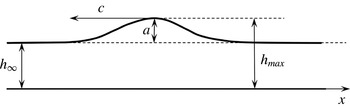
We consider a solitary wave propagating with a negative celerity $c$ in the direction of decreasing $x$ in still water of depth $h_{\infty }$ . The amplitude $a$ of the wave is defined as

(4.1) $$\begin{eqnarray}a=h_{max}-h_{\infty },\end{eqnarray}$$

where $h_{max}$ is the maximum depth that is reached under the wave crest (see figure 2). This solitary wave will be studied in a reference frame propagating at the same velocity $c$ as the wave. In this reference frame, the solitary wave is stationary. For $x\rightarrow -\infty$ or $x\rightarrow +\infty$ , the depth is $h_{\infty }$ and the fluid velocity is $U_{\infty }=-c>0$ . Also, the bottom wall moves in this reference frame with the velocity $U_{\infty }$ . We choose, in this reference frame, $x=0$ at the wave crest.

Figure 2.

Notation used for the description of the solitary wave.

We can note that there is a similarity between the propagation of a bore and that of a solitary wave, in that in both cases the fluid is initially quiescent and thus irrotational, and that the vorticity is created at the wavefront. The similarity between weak hydraulic jumps and spilling breakers in the inner surf-zone in a reference frame moving with the broken wave has been highlighted, for example, by Dabiri & Gharib (Reference Dabiri and Gharib1997) and Misra et al. (Reference Misra, Kirby, Brocchini, Veron, Thomas and Kambhamettu2008).

Of course, because of friction at the bottom, vorticity is generated as soon as the wave comes, in a thin boundary layer (the flow can be considered as non-developed). However, if a turbulent structure appears, it appears in the upper part of the flow and the vorticity at the bottom can hardly explain the phenomenon.

Dabiri & Gharib (Reference Dabiri and Gharib1997) investigated experimentally the vorticity generation within a spilling water wave. They concluded also that the spilling breaker can be modelled as a local hydraulic jump. They found that the source of vorticity is mainly due to the free-surface deceleration. According to them, ‘the free-surface deceleration not only produces a vorticity flux into the flow through a diffusive process, but in doing so, simultaneously generates a sharp slip velocity which grows into a shear layer, convecting downstream the vorticity which is fluxed into the fluid from the free surface’. They also pointed out that ‘the location of maximum deceleration, and therefore the flux of vorticity into the flow, are clearly distinguishable from the location of the stagnation point along the free surface and the onset of separation from the surface’ (note that the stagnation point indicates the breaking of the wave).

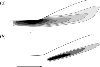
Similar results were found experimentally by Misra et al. (Reference Misra, Kirby, Brocchini, Veron, Thomas and Kambhamettu2008) on a weak hydraulic jump. They wrote that ‘all evidence suggests that breaking is driven by a surface-parallel adverse pressure gradient and a streamwise flow deceleration at the toe of the breaker’ and that ‘the flow characteristics, particularly near the toe and the free surface, depend significantly on the inflow characteristics’. They found that ‘there is a thin concentrated region of negative vorticity in the breaker shear layer’ but that ‘the mean vorticity has its peak, negative value, upstream of the toe … and decreases in the downstream direction’. They noticed that they found a non-zero vorticity at the mean surface. Further, their measurements show that the maximum vorticity is at the free surface, upstream of the jump’s toe, whereas the maximum turbulent energy is at the toe of the breaker. The turbulence structure of the breaker shear layer resembles that of a mixing layer originating from the toe of the breaker. From this point, the turbulence intensity decays rapidly away (Misra et al. Reference Misra, Kirby, Brocchini, Veron, Thomas and Kambhamettu2008). The turbulent energy in the reverse-flow region above the shear layer of the breaker is an order of magnitude smaller than in the shear layer (Misra et al. Reference Misra, Kirby, Brocchini, Veron, Thomas and Kambhamettu2008). Figure 3 shows a sketch of the strong vorticity areas and of the strong turbulent energy areas in the weak hydraulic jump studied by Misra et al. (Reference Misra, Kirby, Brocchini, Veron, Thomas and Kambhamettu2008).

Figure 3.

(a) Sketch of the averaged vorticity for a weak hydraulic jump (after Misra et al. Reference Misra, Kirby, Brocchini, Veron, Thomas and Kambhamettu2008) in the upper portion of the flow. The upstream Froude number is 1.2. Darker areas indicate a stronger vorticity. Maximum vorticity is found before the toe of the jump. (b) Sketch of the turbulent kinetic energy in this same hydraulic jump (after Misra et al. Reference Misra, Kirby, Brocchini, Veron, Thomas and Kambhamettu2008). Darker areas indicate a larger turbulence intensity.

Finally, it appears that a strong vorticity is generated along the air–water interface. With our choice of the reference frame moving with the wave, this vorticity is negative. For our model, this implies a non-zero, negative value of $A$ before the wave. It can be easily proved that if $\partial u_{1}/\partial z>0$ then $A>0$ , and that if $\partial u_{1}/\partial z<0$ then $A<0$ . As we assumed $\partial u_{1}/\partial z={\it\omega}$ , the sign of ${\it\omega}$ is the sign of $A$ . Note that, in our case, the vorticity at the thin bottom boundary layer is also negative and that above this boundary layer but beneath the upper shear layer at the air–water interface, the vorticity is very small and can be considered equal to zero. We can model this as (3.19)–(3.21) (see § 3.4.1) and take the expression (3.23) for $A$ with $A_{0}<0$ . The fact that the maximum of the turbulent energy appears after the maximum of the vorticity is an argument in favour of a generation of turbulent enstrophy ${\it\Phi}$ caused by the presence of vorticity implied by the non-zero value of $A$ . The shear vorticity in the thin layer close to the air–water interface can be partially transformed into turbulent vorticity related to rapidly varied motions.

4.2. Explicit expression of the wave profile

Let us consider solutions of (2.60)–(2.64) with (3.23) depending only on ${\it\xi}=x-ct$ . Since these equations are Galilean invariant, it is equivalent to looking for stationary solutions. Thus, the balance equation for mass leads to the conservation of the discharge $q$ :

(4.2) $$\begin{eqnarray}q=hU=\text{constant}.\end{eqnarray}$$

Instead of (2.62), we can take (3.25) with the approximation (3.26). This gives in the stationary case

(4.3) $$\begin{eqnarray}{\it\Phi}={\it\varphi}+\frac{2A_{0}q}{h^{3}}\left[\frac{\text{d}^{2}h}{\text{d}x^{2}}-\frac{1}{h}\left(\frac{\text{d}h}{\text{d}x}\right)^{2}\right],\end{eqnarray}$$

where ${\it\varphi}={\it\Phi}_{\infty }$ is the turbulent enstrophy far from the wave (for $x\rightarrow \pm \infty$ ). In fact, ${\it\varphi}$ should be zero as the fluid is initially quiescent, but a very small value of ${\it\Phi}$ is generated immediately by the wave, whether at the bottom boundary layer due to friction or at the air–water interface.

The equations are put in dimensionless form as in (2.8) and (2.26) with $H=h_{\infty }$ . Further, $\tilde{x}=x/h_{\infty }$ and the Froude number is defined as

(4.4) $$\begin{eqnarray}F=q/\sqrt{gh_{\infty }^{3}}.\end{eqnarray}$$

We can also write this Froude number as $F=U_{\infty }/\sqrt{gh_{\infty }}$ or $F=|c|/\sqrt{gh_{\infty }}$ . It is the dimensionless wave velocity. We also have

(4.5) $$\begin{eqnarray}\tilde{A}_{0}=\frac{A_{0}}{\sqrt{gh_{\infty }^{3}}}.\end{eqnarray}$$

The integration of this system gives an explicit dimensionless expression for the solitary wave,

(4.6) $$\begin{eqnarray}\tilde{h}=1+\frac{2\tilde{a}(F^{2}-1-3\tilde{{\it\varphi}})}{F^{2}-1-(3+\tilde{a}^{2})\tilde{{\it\varphi}}+[F^{2}-1-(3-\tilde{a}^{2})\tilde{{\it\varphi}}]\,\text{ch}\left[\tilde{x}\sqrt{3{\displaystyle \frac{F^{2}-1-3\tilde{{\it\varphi}}}{F^{2}+18\tilde{A}_{0}F}}}\right]},\end{eqnarray}$$

where $\tilde{a}=a/h_{\infty }$ is the dimensionless amplitude of the solitary wave. It is obvious from this expression that a solitary wave can only exist if

(4.7) $$\begin{eqnarray}F>\sqrt{1+3\tilde{{\it\varphi}}}.\end{eqnarray}$$

For the Green–Naghdi model, this condition was simply $F>1$ . In our model, the long wave velocity $\sqrt{gh}$ has to be replaced by $\sqrt{gh+3h^{2}{\it\Psi}}$ (Teshukov Reference Teshukov2007; Richard & Gavrilyuk Reference Richard and Gavrilyuk2012). The Froude number, which is the ratio of the fluid velocity to the long wave velocity, has to be replaced by the generalized Froude number

(4.8) $$\begin{eqnarray}F_{g}=\frac{U}{\sqrt{gh+3h^{2}{\it\Psi}}}.\end{eqnarray}$$

The condition of existence for solitary waves is simply $F_{g}>1$ .

The expression of the dimensionless amplitude of the solitary wave is

(4.9) $$\begin{eqnarray}\tilde{a}=\frac{1}{2\tilde{{\it\varphi}}}\left[-(1+4\tilde{{\it\varphi}})+\sqrt{(1+4\tilde{{\it\varphi}})^{2}+4(F^{2}-1-3\tilde{{\it\varphi}})\tilde{{\it\varphi}}}\right].\end{eqnarray}$$

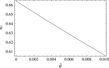
This amplitude decreases if $\tilde{{\it\varphi}}$ increases (see figure 4). It is always smaller than the amplitude of the solitary wave in the Green–Naghdi model, which is $\tilde{a}=F^{2}-1$ . For a non-developed flow, the order of magnitude of $\tilde{{\it\varphi}}$ is $5\times 10^{-3}$ (see Richard & Gavrilyuk Reference Richard and Gavrilyuk2013). Therefore, assuming a small value for $\tilde{{\it\varphi}}$ , $\tilde{a}$ can be developed and the following approximate expression of $\tilde{a}$ can be found:

(4.10) $$\begin{eqnarray}\tilde{a}=F^{2}-1-\tilde{{\it\varphi}}F^{2}(2+F^{2})+2\tilde{{\it\varphi}}^{2}F^{2}(2+3F^{2}+F^{4})+O(\tilde{{\it\varphi}}^{3}).\end{eqnarray}$$

The amplitude of the solitary wave of Boussinesq is also $\tilde{a}=F^{2}-1$ . The solitary waves of the Korteweg–de Vries equation have an amplitude $\tilde{a}=2(F-1)$ . Grimshaw (Reference Grimshaw1971) found $F=\sqrt{1+\tilde{a}-\tilde{a}^{2}/20-3\tilde{a}^{3}/70}$ . It is well known that the celerity of the solitary wave found by Boussinesq or by Su & Gardner (Reference Su and Gardner1969) (Green–Naghdi model), and even more by the Korteweg–de Vries equation, is slightly higher than the experimental values (Daily & Stephan Reference Daily and Stephan1952), especially for solitary waves of high amplitude ( $\tilde{a}>0.5$ ). On the other hand, the expression of Grimshaw (Reference Grimshaw1971) is in very good agreement with the experimental values. Since the value of $F$ that we found for a given amplitude is slightly higher than the value given by the Green–Naghdi model because of $\tilde{{\it\varphi}}$ , the result we found is also slightly worse than the Green–Naghdi model with respect to the relation between the wave celerity and its amplitude. We currently believe that this discrepancy is due to the irrotational term, which was neglected since the inclusion of higher-order terms leads to an improvement of this relation (for example Grimshaw Reference Grimshaw1971; Fenton Reference Fenton1972; Shields & Webster Reference Shields and Webster1988 and, specifically for the irrotational Green–Naghdi model, Kim et al. Reference Kim, Bai, Ertekin and Webster2003).

Figure 4.

Variation of the dimensionless amplitude $\tilde{a}$ of the solitary wave with $\tilde{{\it\varphi}}$ for $F=1.29$ .

Experimental profiles of solitary waves have been found by various authors, notably by Daily & Stephan (Reference Daily and Stephan1952). They compared the experimental profiles to theoretical profiles, especially the profile found by Boussinesq (Reference Boussinesq1872),

(4.11) $$\begin{eqnarray}\tilde{h}=1+\tilde{a}\;\text{sec}\text{h}^{2}\left(\tilde{x}\sqrt{{\textstyle \frac{3}{4}}\tilde{a}}\right),\end{eqnarray}$$

and the profile found by Rayleigh (1876), which has the same expression as the profile found by Su & Gardner (Reference Su and Gardner1969)

(4.12) $$\begin{eqnarray}\tilde{h}=1+\tilde{a}\;\text{sec}\text{h}^{2}\left(\tilde{x}\sqrt{\frac{3}{4}\frac{\tilde{a}}{1+\tilde{a}}}\right).\end{eqnarray}$$

They concluded that the Boussinesq profile gives the most consistent agreement with the experimental values.

It can be noted that, if $\tilde{{\it\varphi}}=0$ , the profile found (4.6) reduces to

(4.13) $$\begin{eqnarray}\tilde{h}=1+\tilde{a}\;\text{sec}\text{h}^{2}\left[\tilde{x}\sqrt{\frac{3}{4}\;\frac{\tilde{a}}{1+\tilde{a}+18\tilde{A}_{0}\sqrt{\tilde{a}+1}}}\right].\end{eqnarray}$$

Further, if $\tilde{A}_{0}=0$ , this profile reduces to the Rayleigh and Su–Gardner profile. On the other hand, if

(4.14) $$\begin{eqnarray}\tilde{A}_{0}=-\frac{\tilde{a}}{18\sqrt{\tilde{a}+1}},\end{eqnarray}$$

the profile we found reduces to the Boussinesq profile. If $\tilde{{\it\varphi}}=0$ , the amplitude (4.9) becomes simply $\tilde{a}=F^{2}-1$ . Hence, this condition (4.14) can also be written as

(4.15) $$\begin{eqnarray}\tilde{A}_{0}=\frac{1-F^{2}}{18F}.\end{eqnarray}$$

Our goal here is to handle turbulence generation rather than to fit the experimental profiles. For the latter task, the irrotational term has to be taken into account. However, this model is able to give profiles in very good agreement with the experimental profiles. As was discussed previously, we take the expression (3.23) with $\tilde{A}_{0}<0$ . We could adjust the value of $\tilde{A}_{0}$ in order to get the best agreement with the experimental profiles. 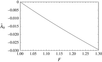As we only need an approximate value of $\tilde{A}_{0}$ for our goal, we will use (4.15) in order to get the Boussinesq profile, which has already been found to be in good agreement with the experiments. The values of $\tilde{A}_{0}$ are plotted in figure 5 as a function of $F$ .

Figure 5.

Values of $\tilde{A}_{0}$ as a function of the Froude number $F$ from (4.15).

With the value of $\tilde{A}_{0}$ and $\tilde{{\it\varphi}}$ , the profile can be derived from (4.6). It is then possible to solve (4.3) to find the evolution of the enstrophy in the wave. Starting from $\tilde{{\it\varphi}}$ for $\tilde{x}\rightarrow -\infty$ , the enstrophy first decreases and then increases to a value greater than $\tilde{{\it\varphi}}$ which is maximum for $\tilde{x}=0$ , then follows a symmetrical behaviour for $\tilde{x}>0$ . If $\tilde{{\it\varphi}}$ is too small, the enstrophy can become negative, which is of course not possible. 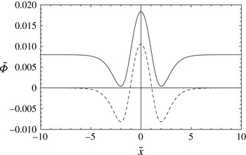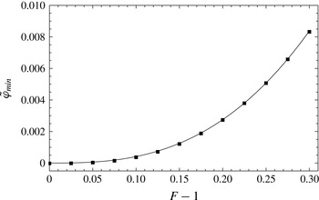If $\tilde{{\it\varphi}}$ has a greater value, the curve of $\tilde{{\it\Phi}}$ as a function of $\tilde{x}$ is simply translated towards higher values of $\tilde{{\it\Phi}}$ , as shown in figure 6. The minimal value of $\tilde{{\it\varphi}}$ which guarantees a positive value of $\tilde{{\it\Phi}}$ as a function of the Froude number can then be found. This expression is not explicit, even if the corresponding numerical procedure for finding $\tilde{{\it\varphi}}_{min}$ is simple. These values are plotted in figure 7.

Figure 6.

Profiles of the enstrophy in a solitary wave as a function of $\tilde{x}$ for $F=1.29$ if $\tilde{{\it\varphi}}=0$ (dashed curve) and if $\tilde{{\it\varphi}}=0.008$ (solid line). In each case, $\tilde{A}_{0}$ is found with (4.15), which gives $\tilde{A}_{0}=-0.0286$ .

Figure 7.

Values of the minimal value of $\tilde{{\it\varphi}}$ as a function of $F-1$ .

The numerical values of $\tilde{{\it\varphi}}_{min}$ are of the same order of magnitude as those estimated in Richard & Gavrilyuk (Reference Richard and Gavrilyuk2013) for hydraulic jumps with a non-developed inflow. Knowing $\tilde{A}_{0}$ with (4.15) and taking the corresponding value as $\tilde{{\it\varphi}}=\tilde{{\it\varphi}}_{min}$ , it is possible to calculate the profiles of solitary waves and to find the relation between the dimensionless wave celerity $F$ and the dimensionless wave amplitude $\tilde{a}$ . 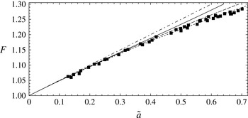The relation between $F$ and $\tilde{a}$ is plotted in figure 8 and compared with experimental results from Watanabe (Reference Watanabe2007) and other theoretical solutions. The solution of Grimshaw (Reference Grimshaw1971) is in very good agreement with the experimental results. The other solutions overestimate the celerity for a given amplitude, or, equivalently, underestimate the amplitude for a given Froude number. The expressions of Boussinesq and Rayleigh (Su–Gardner, Green–Naghdi model) are in good agreement with the experiments for $\tilde{a}<0.5$ . Our solution gives higher wave velocities and is in good agreement with the measurements for $\tilde{a}<0.4$ . The Korteweg–de Vries equation gives the right value of the wave celerity only for small-amplitude waves (as expected), for $\tilde{a}<0.2$ . Our result falls between the Green–Naghdi model and the Korteweg–de Vries equation.

Figure 8.

Relation between the dimensionless wave velocity $F$ and the dimensionless wave amplitude $\tilde{a}$ . Squares, experimental measures of Watanabe (Reference Watanabe2007); solid line, our result with (4.15),  $\tilde{{\it\varphi}}=\tilde{{\it\varphi}}_{min}$ ; long dashed line, Boussinesq and Rayleigh (and also Su & Gardner Reference Su and Gardner1969, Green–Naghdi model) solutions; short dashed line, solution of Grimshaw (Reference Grimshaw1971); dot-dashed line, solution of the Korteweg–de Vries equation.

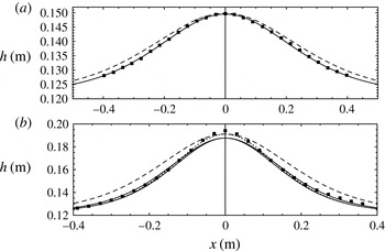
The calculated profiles of solitary waves are then compared to experimental results obtained by Daily & Stephan (Reference Daily and Stephan1952). Two cases are presented in figure 9. The first one is a case of a small-amplitude wave with $F=1.11$ and $\tilde{a}=0.23$ . The value of $\tilde{A}_{0}$ is $-0.0116$ and $\tilde{{\it\varphi}}=0.000533$ . The profile we obtained is in very good agreement with the experimental profile and is an improvement on the Rayleigh profile. It is nearly identical to the Boussinesq profile by the choice of (4.15). The second case is that of a large-amplitude wave with $F=1.25$ and $\tilde{a}=0.6$ . The profile was calculated with $\tilde{A}_{0}=-0.0252$ and $\tilde{{\it\varphi}}=0.00519$ . The calculated profile is also an improvement on the Rayleigh profile except near the maximum depth of the wave, which is not sharp enough. Apart from the top region of the wave, the profile is in good agreement with the experiment. The calculated profile is better than the profile found with the Green–Naghdi model everywhere except in the area of the top of the wave. In particular, the width of the solitary wave, which is slightly too wide with the Green–Naghdi model, is in much better agreement with our model. The top area of the wave is likely to be improved in our model by the inclusion of the irrotational term, as noted above from the results obtained by various authors, especially Kim et al. (Reference Kim, Bai, Ertekin and Webster2003). The profile could even be improved by a choice of $\tilde{A}_{0}$ different from (4.15). For example, $\tilde{A}_{0}=-0.020$ gives even better results (but the top region is not improved). The value of $\tilde{A}_{0}$ , does not change the wave amplitude, which depends only on $F$ and $\tilde{{\it\varphi}}$ , but modifies the width of the wave. With $\tilde{A}_{0}>0$ , the solitary wave is wider by comparison with the Rayleigh solitary wave profile, and with $\tilde{A}_{0}<0$ it is narrower. For all values of $F$ , the Rayleigh profile is slightly too wide. With $\tilde{A}_{0}<0$ , the profile is closer to the experimental profile, except at the top region of the largest waves.

Figure 9.

Profiles of solitary waves. (a) Small-amplitude wave with $F=1.11$ , $\tilde{a}=0.23$ . Squares, experimental measures of Daily & Stephan (Reference Daily and Stephan1952); solid line, calculated profile with $\tilde{A}_{0}=-0.0116$ and $\tilde{{\it\varphi}}=0.000533$ ; dashed line, Rayleigh profile (also Su & Gardner Reference Su and Gardner1969). (b) Large-amplitude wave with $F=1.25$ and $\tilde{a}=0.6$ . Squares, experimental measures of Daily & Stephan (Reference Daily and Stephan1952); thick solid line, calculated profile with $\tilde{A}_{0}=-0.0252$ and $\tilde{{\it\varphi}}=0.00519$ ; thin solid line, calculated profile with $\tilde{A}_{0}=-0.020$ and $\tilde{{\it\varphi}}=0.00519$ ; long dashed line, Rayleigh profile (also Su & Gardner Reference Su and Gardner1969); short dashed line, Boussinesq profile.

The explicit stationary solution was found with $A=A_{0}h^{2}$ . It is worth noting that stationary solitary wave solutions exist for any dependence of $A$ on $h$ , even if they are not explicit. In this general case, the equation for the fluid depth is

(4.16) $$\begin{eqnarray}-\left(\frac{q^{2}}{3}+\frac{4qA}{h^{2}}\right)\frac{\text{d}^{2}}{\text{d}x^{2}}\left(\frac{1}{h}\right)+\frac{\text{d}}{\text{d}x}\left(\frac{q}{h^{3}}\frac{\text{d}A}{\text{d}x}\right)=\frac{3m}{h^{2}}-\frac{2b}{h}-\frac{2q^{2}}{h^{3}}+\frac{g}{2},\end{eqnarray}$$

where $m$ and $b$ are the constants

(4.17) $$\begin{eqnarray}\displaystyle & \displaystyle m=\frac{q^{2}}{h_{\infty }}+\frac{gh_{\infty }^{2}}{2}+h_{\infty }^{3}{\it\varphi}, & \displaystyle\end{eqnarray}$$

(4.18) $$\begin{eqnarray}\displaystyle & \displaystyle b=\frac{q^{2}}{2h_{\infty }^{2}}+gh_{\infty }+\frac{3}{2}h_{\infty }^{2}{\it\varphi}. & \displaystyle\end{eqnarray}$$

$A=A_{0}h^{2}$

4.3. Turbulence generation

Having determined the values of $\tilde{A}_{0}$ and $\tilde{{\it\varphi}}$ , the variations of the turbulent enstrophy can now be calculated in order to study the generation of turbulence. The experimental maximum value of the dimensionless amplitude of a solitary wave is related to the breaking of the wave. For a breaking wave, not only is there a turbulent structure but also the wave profile becomes asymmetric, and there is dissipation producing a decrease in both the amplitude and the velocity of the wave. McCowan (Reference McCowan1894) predicted a maximum dimensionless amplitude of $\tilde{a}=0.78$ , which is slightly higher than the experimental value measured by Watanabe (Reference Watanabe2007) of $\tilde{a}=0.70$ . The experimental maximum dimensionless velocity is $F=1.29$ (Watanabe Reference Watanabe2007). The determination of the value of the maximum wave amplitude assumes that the velocity of a particle at the crest is equal to the velocity of the wave, and that the free surface forms a point at the crest with an angle of $2{\rm\pi}/3$ . However, Watanabe (Reference Watanabe2007) observed no overturning of the wave crest above the critical value of the amplitude but the appearance of a turbulent structure of a micro type (micro instability).

The calculation of the variation of enstrophy with $\tilde{x}$ shows that the value of the enstrophy reached a maximum at the peak of the wave. This maximum increases with the Froude number $F$ . It was shown in Richard & Gavrilyuk (Reference Richard and Gavrilyuk2013) that the disappearance of the roller of a hydraulic jump can be related to a critical value of the dimensionless enstrophy. This threshold was found to be in very good agreement with experimental measures of the roller length of hydraulic jumps at any upstream Froude number. In the present case of the solitary wave, we propose that the onset of the instability of the wave, i.e. the breaking of the wave, is related to the crossing of a threshold by the enstrophy. As long as the enstrophy is smaller than a critical value, the solitary wave is stable and no turbulent structure appears. If the value of the enstrophy becomes greater than this critical value, the wave breaks and dissipation appears, which makes the wave asymmetric and unstable.

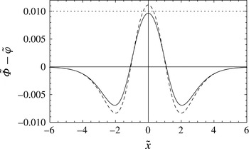
This critical value of the enstrophy can be estimated by the maximum value reached by $\tilde{{\it\Phi}}-\tilde{{\it\varphi}}$ at the critical Froude number of $F=1.29$ . As usual, $\tilde{A}_{0}$ is given by (4.15), and $\tilde{{\it\varphi}}$ corresponds to $\tilde{{\it\varphi}}_{min}$ . In figure 10, the variation of $\tilde{{\it\Phi}}-\tilde{{\it\varphi}}$ is plotted in the case of a stable solitary wave with $F=1.28$ , just below the critical value, and in the case of an unstable wave with $F=1.30$ , slightly above the critical value. The critical value of $\tilde{{\it\Phi}}-\tilde{{\it\varphi}}$ is approximately 0.010. It is also possible to look for a critical value of $\tilde{{\it\Phi}}$ instead of $\tilde{{\it\Phi}}-\tilde{{\it\varphi}}$ , in which case a value close to 0.018 is found.

Figure 10.

Variations of the dimensionless enstrophy $\tilde{{\it\Phi}}-\tilde{{\it\varphi}}$ in the solitary wave as a function of $\tilde{x}$ . Solid line, case $F=1.28$ , $\tilde{A}_{0}=-0.0277$ , $\tilde{{\it\varphi}}=0.00692$ ; dashed line, case $F=1.30$ , $\tilde{A}_{0}=-0.0295$ , $\tilde{{\it\varphi}}=0.00837$ ; dotted horizontal line, $\tilde{{\it\Phi}}-\tilde{{\it\varphi}}=0.010$ .

Once breaking is reached, dissipation effects appear that are not included in the present model. It is thus not possible to describe these breaking waves without having introduced the dissipation in the equations. We believe that the present model is able to predict the onset of breaking but that it has to be augmented to handle the case of breaking waves. The dissipative terms included in Richard & Gavrilyuk (Reference Richard and Gavrilyuk2013) are likely to be included in the future dissipative and dispersive model for breaking waves.