



1 Introduction
Viscous fingering occurs when a low-viscosity fluid is used to displace a more viscous fluid through a porous medium. The phenomenon is of considerable importance for the oil industry since it can lead to injected water bypassing the oil in a reservoir, with the result that there are large pockets of unswept oil (Lake Reference Lake1989; Woods Reference Woods2015). The injection of a less viscous fluid into a more viscous fluid in a Hele-Shaw cell is also subject to viscous fingering. If pore-scale physics and two-phase flow effects are neglected, then the Hele-Shaw cell can be used as a two-dimensional analogue model of a porous medium. We adopt this approach herein, and the remainder of the paper focuses on Hele-Shaw flows.
A variety of approaches to control the stability of the interface have been explored. They can be classed as involving modification of (1) the Hele-Shaw cell geometry, (2) the injection flow rate, (3) fluid properties or (4) combinations thereof. For the first class, Al-Housseiny & Stone (Reference Al-Housseiny and Stone2013) performed a linear stability analysis for flow in a tapering cell, and experimentally verified how the tapering angle modified the stability of the interface, whereas Pihler-Puzović et al. (Reference Pihler-Puzović, Illien, Heil and Juel2012) investigated the stabilising effect of replacing the top plate with an elastic membrane. Zheng, Kim & Stone (Reference Zheng, Kim and Stone2015) defined a control parameter that, if held constant in time, permits selection of which azimuthal mode is manifest throughout the injection. In that study, the control parameter was held constant by varying the gap thickness,
 $b$
, according to
 $b(t)\sim t^{1/7}$
. In a different study, the control parameter was held constant by varying the injection flow rate,
 $Q$
, according to
 $Q(t)\sim t^{-1/3}$
(Li et al.
Reference Li, Lowengrub, Fontana and Palffy-Muhoray2009). Both studies demonstrated good agreement between experiment and theoretical prediction of the dominant mode of instability that develops. For the latter case, Dias & Miranda (Reference Dias and Miranda2010) went on to perform a weakly nonlinear mode-coupling analysis to explain how the
 $Q\sim t^{-1/3}$
injection flow rate leads to sharpening, stable fingers.
Modification of the fluids (class (3) above) has also been shown to give interfacial control. The viscosity of the injected fluid can be increased, for example by adding a polymer (Sorbie Reference Sorbie1991). Since the field-scale deployment of polymer can be expensive, in some cases a finite volume of polymer solution is injected between the oil and the water. This leads to a series of interesting problems concerning the stability of a flood front with two interfaces, and an analysis has been presented for this coupled problem based on flow in a Hele-Shaw cell (Cardoso & Woods Reference Cardoso and Woods1995). Gorell & Homsy (Reference Gorell and Homsy1983) generalised the two-interface analysis by exploring the stability of a unidirectional constant flow in which the concentration of injected polymer varies with position in the flow. They developed a variational approach to determine the optimal concentration of the injected polymer as a function of time in order to minimise the viscous instability when finite masses of polymer and water are injected. Following a different approach, Gin & Daripa (Reference Gin and Daripa2015) calculated the stability of a series of discrete layers of different viscosity injected in sequence. However, there are challenges associated with the direct injection of polymer solutions into a porous medium, including the risk that the polymer may block up pore throats near the injector and hence prevent the continued injection of fluid into the reservoir in order to displace the oil (Sorbie Reference Sorbie1991; Woods Reference Woods2015). In order to mitigate such risks, it is possible to use a polymer with a delayed activation so that the mixture viscosity gradually increases with time.
There are a variety of methods that could achieve this. For example, if the polymer is supplied in a soluble encapsulant with a finite release time, then the concentration of polymer in solution would gradually change as the encapsulant dissolves. Gun & Routh (Reference Gun and Routh2013) explored the possibility of using poly(lactic-co-glycolic) acid to encapsulate a gelling agent that is gradually released. In the context of drug delivery in the body, Makadia & Siegel (Reference Makadia and Siegel2011) detail how the release profile of this encapsulant can be tuned by varying the composition. Alternatively, the polymer may be thermally activated, gelling once it passes through an activation temperature. Tran-viet, Routh & Woods (Reference Tran-viet, Routh and Woods2014) explored the thermal response of poly
 $N$
-isopropylacrylamide to this end. The viscosity may also vary on account of reaction. Polyacrylamide (PAA) solutions are commonly used in oil field displacements (Kamal et al.
Reference Kamal, Sultan, Al-Mubaiyedh and Hussein2015). In addition to gradual release from encapsulant, time dependence can be introduced to PAA solution viscosity through tailoring reaction kinetics. Han et al. (Reference Han, Shi, Ye and Ma1995) demonstrated that the addition of chromium ions to PAA led to the formation of a cross-linked gel structure, and that the addition of acetic acid to this solution delayed the rate of gel formation. Furthermore, we hypothesise that, by limiting the initial concentration of chromium ions, the rheological properties of the final polymer solution, including the cross-links, can also be controlled. In the case of PAA polymerisation, Lee et al. (Reference Lee, Morad, Teng and Poh2012) measured the gradual change in solution viscosity over the course of the reaction and demonstrated that the rate of reaction is dependent on the concentration of various reagents. With polymer solutions (including those of PAA), shear can cause the polymer chains to align, which can lead to a decrease in the effective viscosity. Thus, polymer solutions with time-dependent viscosity may exhibit shear-thinning behaviour.
Drawing on the results of previous work related to time-dependent changes in viscosity, we now explore how such variations of viscosity may impact the stability of a moving interface, and, given the evolving rheology, we also account for possible variations in injection rate. Such effects may be key for the class of problem in which a finite volume of fluid is to be injected in a finite time, and in this case there is the intriguing possibility that, by varying the flow rate with time, the final amplitude of instability can be further reduced. In exploring this class of problem, we are guided by the pioneering works of Dias, Parisio & Miranda (Reference Dias, Parisio and Miranda2010) and Dias et al. (Reference Dias, Alvarez-Lacalle, Carvalho and Miranda2012), who examined the impact of changes in flow rate on the growth of viscous fingers. In particular, Dias et al. (Reference Dias, Alvarez-Lacalle, Carvalho and Miranda2012) considered the problem of injection of a finite volume of fluid in a finite time, and, using variational calculus, developed an expression for the injection flow rate as a function of time which minimises the final amplitude of instability.
We have arranged the paper as follows. In § 2 we consider the impact of time-dependent rheology in a unidirectional displacement of Newtonian fluids, in which there is a continuous range of unstable wavenumbers. We assess the relationship between the time-dependent viscosity of the injected fluid and the optimal injection rate. In § 3 we extend the results to consider injection from a central source in which the instability leads to a discrete series of modes with increasing azimuthal wavenumber,
 $n$
, of the form
 $A_{n}(t)\exp (\text{i}n\unicode[STIX]{x1D703})$
(cf. Paterson Reference Paterson1981). In this case, the analysis is more complex owing to the continual stretching of the interface, which progressively suppresses the instability of lowest modes as the interface grows, while surface tension suppresses the instability of the highest modes (cf. Cardoso & Woods Reference Cardoso and Woods1995). In order to make progress, following Dias et al. (Reference Dias, Alvarez-Lacalle, Carvalho and Miranda2012) we approximate the discrete spectrum of modes with a continuous spectrum, noting that this will lead to an upper bound on the actual growth rate. We find that, for a given initial radius
 $R_{0}$
, there is a particular total injection time,
 $t_{f}^{\dagger }$
, for which the system is just stable, provided the injection rate decreases with time according to
 $Q=a(b+ct)^{-1/3}$
, where the constants
 $a,~b$
and
 $c$
are found in our analysis. If
 $t_{f}$
decreases to values
 $t_{f}<t_{f}^{\dagger }$
, for this given
 $R_{0}$
, then the optimal injection rate gradually evolves towards the simple linearly increasing rate
 $Q=d+et$
, where
 $d$
and
 $e$
again are found from the analysis. This limit coincides with the results of Dias et al. (Reference Dias, Alvarez-Lacalle, Carvalho and Miranda2012), who investigated the optimal injection rate in the limit
 $t_{f}\ll t_{f}^{\dagger }$
. We then illustrate how a gradual increase in the viscosity of the injected fluid, for example resulting from slow activation of gel, modifies this optimal solution so that, as for the unidirectional flow, the optimal injection rate increases with time from a smaller to a larger value than for the case in which the injected fluid has a constant viscosity equal to the initial viscosity. Given that many polymer solutions exhibit shear-thinning rheology, in § 4 we generalise the analysis to account for such rheology in the calculation of the optimal flow rate with time. Earlier work has explored aspects of the stability of non-Newtonian fluids as they are displaced through a Hele-Shaw cell. In particular, Wilson (Reference Wilson1990) developed the dispersion relation for the case in which air displaces a non-Newtonian fluid through a rectilinear geometry and this work was developed to describe the stability of a radially spreading front by Sader, Chan & Hughes (Reference Sader, Chan and Hughes1994). In the present work, we explore a different problem in which a non-Newtonian fluid displaces a more viscous Newtonian fluid through a rectilinear geometry. It is noted that the more complicated configuration in which both fluids are non-Newtonian has been considered by Martyushev et al. (Reference Martyushev, Birzina, Konovalov and Sergeev2015) for the axisymmetric geometry and, in a different study, the stability of a bubble contracting towards a point sink surrounded by a power-law fluid was considered by McCue & King (Reference McCue and King2011). We explore the control implications of the nonlinear rheology and compare our results to Fontana, Dias & Miranda (Reference Fontana, Dias and Miranda2014), who generalised the analysis of Dias et al. (Reference Dias, Alvarez-Lacalle, Carvalho and Miranda2012) to the case in which air displaces a shear-thinning fluid. In comparison with the Newtonian case, Fontana et al. (Reference Fontana, Dias and Miranda2014) found that the optimal injection rate involves a more rapid injection at early times and slower injection later. Finally, in a discussion section of the paper, we summarise our key results and draw some conclusions about the efficacy of the control strategies identified herein.
2 Rectilinear channel flow of Newtonian fluids
2.1 Formulation
The depth-averaged flow of fluid in a Hele-Shaw cell is governed by the following equations (Saffman & Taylor Reference Saffman and Taylor1958):
 $$\begin{eqnarray}\unicode[STIX]{x1D735}\boldsymbol{\cdot }\boldsymbol{u}=0\quad \text{and}\quad \boldsymbol{u}=-\frac{b^{2}}{12\unicode[STIX]{x1D707}}\unicode[STIX]{x1D735}p,\end{eqnarray}$$
where
 $\boldsymbol{u}$
denotes velocity,
 $b$
is the plate separation,
 $\unicode[STIX]{x1D707}$
is the viscosity of the fluid and
 $p$
is the pressure.
By applying the interfacial boundary conditions of conservation of velocity and the jump in pressure on account of interfacial tension, and exploring the stability of the interface to small sinusoidal perturbations along the interface, Saffman & Taylor (Reference Saffman and Taylor1958) obtained the dispersion relation
 $$\begin{eqnarray}\frac{{\dot{A}}}{A}=\unicode[STIX]{x1D70E}_{k}=\frac{\unicode[STIX]{x1D707}_{2}-\unicode[STIX]{x1D707}_{1}}{\unicode[STIX]{x1D707}_{2}+\unicode[STIX]{x1D707}_{1}}Uk-\frac{b^{2}T}{12(\unicode[STIX]{x1D707}_{1}+\unicode[STIX]{x1D707}_{2})}k^{3},\end{eqnarray}$$
where
 $T$
is the interfacial tension,
 $A(k,t)$
is the amplitude of a perturbation of wavenumber
 $k$
,
 $U(t)$
is the velocity of the interface and subscript
 $1$
denotes the displacing fluid whereas subscript
 $2$
is the displaced fluid. With injection of a finite volume of fluid in a finite time
 $t_{f}$
, such that the interface migrates a distance
 $x_{f}$
, this relation may be expressed in dimensionless form as
 $$\begin{eqnarray}\hat{\unicode[STIX]{x1D70E}_{k}}=\frac{(1-V)\hat{U} \hat{k}-\unicode[STIX]{x1D70F}\hat{k}^{3}}{1+V},\end{eqnarray}$$
where the hat notation denotes a dimensionless variable,
 $\hat{k}=kx_{f}$
,
 $\hat{t}=t/t_{f}$
, the control parameter
 $\unicode[STIX]{x1D70F}=b^{2}Tt_{f}/(12\unicode[STIX]{x1D707}_{2}x_{f}^{3})$
,
 $\hat{U} (\hat{t})=Ut_{f}/x_{f}$
,
 $\hat{\unicode[STIX]{x1D70E}}=\unicode[STIX]{x1D70E}t_{f}$
and
 $V(\hat{t})=\unicode[STIX]{x1D707}_{1}(\hat{t})/\unicode[STIX]{x1D707}_{2}$
. We now drop the hat notation for convenience and henceforth work with dimensionless variables. The wavenumber,
 $k_{max}$
, with maximum growth rate,
 $\unicode[STIX]{x1D70E}_{max}$
, is given by
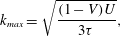 $$\begin{eqnarray}k_{max}=\sqrt{\frac{(1-V)U}{3\unicode[STIX]{x1D70F}}},\end{eqnarray}$$
where
 $$\begin{eqnarray}\unicode[STIX]{x1D70E}_{max}=\frac{2}{3\sqrt{3\unicode[STIX]{x1D70F}}}\frac{(1-V)^{3/2}}{(1+V)}U^{3/2}.\end{eqnarray}$$
At each time, the growth rate of any mode,
 $\unicode[STIX]{x1D70E}(k,t)<\unicode[STIX]{x1D70E}_{max}(t)$
, and so an upper bound on the amplitude of any mode once all the fluid has been injected is given by
 $$\begin{eqnarray}I=\int _{0}^{1}\unicode[STIX]{x1D70E}_{max}\,\text{d}t.\end{eqnarray}$$
In order to find the injection rate,
 $U(t)$
, that minimises
 $I$
subject to the requirement
 $\int _{0}^{1}U\,\text{d}t=1$
, we can follow the Euler–Lagrange framework of variational calculus and seek a solution for
 $U(t)$
of the equation
 $$\begin{eqnarray}\frac{\text{d}}{\text{d}t}\left(\frac{\unicode[STIX]{x2202}\unicode[STIX]{x1D70E}_{max}}{\unicode[STIX]{x2202}U}\right)=0.\end{eqnarray}$$
This leads to the ordinary differential equation (ODE) for
 $U(t)$
,
 $$\begin{eqnarray}(5+V(t))\dot{V}(t)U(t)-(1-V(t)^{2})\dot{U}(t)=0,\end{eqnarray}$$
with solution
 $$\begin{eqnarray}U^{\ast }(t)=\unicode[STIX]{x1D6FA}\frac{(1+V(t))^{2}}{(1-V(t))^{3}},\quad \displaystyle \text{where}~\unicode[STIX]{x1D6FA}=\left(\int _{0}^{1}\frac{(1+V(t))^{2}}{(1-V(t))^{3}}\,\text{d}t\right)^{-1}.\end{eqnarray}$$
If the viscosity ratio is constant,
 $\dot{V}=0$
, then (2.8) predicts that the constant flow,
 $U=1$
, is optimal. It follows that
 $$\begin{eqnarray}k_{max}^{\ast }=\sqrt{\frac{\unicode[STIX]{x1D6FA}}{3\unicode[STIX]{x1D70F}}}\frac{(1+V(t))}{(1-V(t))}\end{eqnarray}$$
and
 $$\begin{eqnarray}\unicode[STIX]{x1D70E}_{max}^{\ast }=\frac{2}{3}\sqrt{\frac{\unicode[STIX]{x1D6FA}^{3}}{3\unicode[STIX]{x1D70F}}}\frac{(1+V(t))^{2}}{(1-V(t))^{3}}.\end{eqnarray}$$
A key parameter in the present model is
 $\unicode[STIX]{x1D70F}$
. Analysis of the upper bound on the amplitude of perturbations, equation (2.6), shows that this may be re-expressed in the form
 $$\begin{eqnarray}A=\exp \left(\int _{0}^{1}f(U,V)\,\text{d}t/\unicode[STIX]{x1D70F}^{1/2}\right),\end{eqnarray}$$
where
 $f(U,V)$
takes on different functional forms depending on whether the injection rate is constant or follows the optimal injection rate. It follows that
 $A^{\sqrt{\unicode[STIX]{x1D70F}}}$
,
 $\sqrt{\unicode[STIX]{x1D70F}}\unicode[STIX]{x1D70E}_{max}$
and
 $\sqrt{\unicode[STIX]{x1D70F}}k_{max}$
are independent of
 $\unicode[STIX]{x1D70F}$
.
2.2 Effect of a gradual increase in viscosity
As mentioned in § 1, the time-dependent viscosity could be tailored through choosing the thickness or composition of polymer micro-encapsulant, altering reagent concentrations to control polymerisation or cross-linking reaction kinetics or altering the temperature to trigger a thermally activated viscosity change. In the case of release from micro-encapsulant, we assume the viscosity of the displacing fluid is directly proportional to the concentration of released polymer and model this concentration as following the release profiles shown in Makadia & Siegel (Reference Makadia and Siegel2011). Thus, the viscosity ratio has the form
 $$\begin{eqnarray}V(t)=V_{0}+(V_{f}-V_{0})(1-\text{e}^{-\unicode[STIX]{x1D703}t}),\end{eqnarray}$$
where
 $V_{0}$
is the initial viscosity ratio,
 $V_{f}$
is the long-time asymptotic viscosity ratio and
 $\unicode[STIX]{x1D703}$
is the ratio of the injection time,
 $t_{f}$
, to the characteristic time for the viscosity change or ‘gelling’. In figure 1(a,b) we illustrate the optimal solutions for the cases in which
 $\unicode[STIX]{x1D703}=1$
, corresponding to slow gelling, and
 $\unicode[STIX]{x1D703}=10$
, corresponding to faster gelling. In both cases, the target change in viscosity of the injected fluid is
 $V_{f}/V_{0}=90$
. In the case
 $\unicode[STIX]{x1D703}=10$
, the viscosity of the injected fluid reaches this target value early in the flow, whereas for the slow gelling case,
 $\unicode[STIX]{x1D703}=1$
, the viscosity is increasing for the duration of the injection. For the faster gelling case,
 $\unicode[STIX]{x1D703}=10$
, the optimal flow rate strategy involves injection of the majority of the fluid once the viscosity has reached its maximum value since adverse viscosity differences are reduced at these later times. In contrast, with slow gelling, the change in viscosity is smaller and so the optimal flow rate increases gradually with time. In figure 1(c,d) we show how the most unstable wavenumber
 $\sqrt{\unicode[STIX]{x1D70F}}k_{max}$
evolves in time, for the optimal flow rate (dashed line), and, for reference, for the case of a constant injection rate (solid line). With a constant flow rate, the most unstable wavenumber decreases with time, owing to the increasing stability of the system. In contrast, the optimal injection profile actually leads to a gradual increase in the most unstable wavenumber with time as a result of the increasing flow rate, even though the viscosity ratio falls with time. As a result of the different evolution of the maximum growth rate with time, we find that, for the optimal flow, the maximum growth rate actually increases with time owing to the progressively faster injection, whereas for a constant injection, the growth rate falls with time (figure 1
e,f).
Results for (a,c,e)
 $\unicode[STIX]{x1D703}=1$
(slow gelling) and (b,d,f)
 $\unicode[STIX]{x1D703}=10$
(rapid gelling). (a,b) Viscosity ratio profiles with parameters
 $\unicode[STIX]{x1D703}$
,
 $V_{0}=0.01$
and
 $V_{f}=0.9$
(primary axis) and the optimal velocity profiles (secondary axis). (c,d) The transition of
 $\sqrt{\unicode[STIX]{x1D70F}}k_{max}$
for the optimal (dashed line) and constant (solid line) flow rate profiles. (e,f) The evolution of
 $\sqrt{\unicode[STIX]{x1D70F}}\unicode[STIX]{x1D70E}$
.

(a) The final amplitude of perturbations of wavenumber
 $k$
for the viscosity invariant case (
 $\unicode[STIX]{x1D703}=0$
, grey) and a gelling case (
 $\unicode[STIX]{x1D703}=1$
) for a constant flow rate (solid line) and the optimal flow rate (broken line). (b) The final maximum amplitudes varying as a function of
 $\unicode[STIX]{x1D703}$
for
 $V_{f}=0.9$
. (c) The ratio of these two final amplitudes as a function of
 $\unicode[STIX]{x1D703}$
for a series of
 $V_{f}$
. (d) The effect of increasing
 $V_{0}$
for a series of
 $V_{f}$
and
 $\unicode[STIX]{x1D703}=2$
. (e) A contour plot of the final amplitude ratio varying with
 $\unicode[STIX]{x1D70F}$
and
 $\unicode[STIX]{x1D703}$
for
 $V_{0}=0.01$
and
 $V_{f}=0.9$
.

We now explore the final amplitude of the perturbation, once the finite volume of fluid has been injected. In order to compare the benefit of the optimal injection rate with the case of constant injection, for different values of
 $\unicode[STIX]{x1D703}$
, it is convenient to investigate the variation of
 $A_{f}^{\sqrt{\unicode[STIX]{x1D70F}}}$
with
 $\unicode[STIX]{x1D703}$
for each case. For clarity, figure 2(a) illustrates the difference between these two amplitudes as a function of wavenumber in the case
 $V_{f}=0.9$
and
 $V_{0}=0.01$
. Figure 2(b) illustrates the ratio of the two final largest amplitudes as a function of
 $\unicode[STIX]{x1D703}$
. Figures 2(a) and 2(b) both illustrate that the maximum benefit arises when
 $\unicode[STIX]{x1D703}$
is close to unity so that the viscosity is changing over the whole period of injection. For small or large
 $\unicode[STIX]{x1D703}$
the difference is much smaller, since in either of these limits the majority of the injection occurs with either the original or the final viscosity. In figure 2(c), curves are given for
 $V_{0}=0.01$
and
 $V_{f}=0.5,~0.7$
and
 $0.9$
corresponding to polymer solutions whose final viscosity is progressively larger. The curves all have a similar shape, but the magnitude of the reduction in amplitude associated with using the optimal injection strategy is greater when the change in viscosity of the polymer gel is greater. This is further illustrated by figure 2(d), which shows how the magnitude of reduction in amplitude diminishes as
 $V_{0}$
approaches
 $V_{f}$
for
 $\unicode[STIX]{x1D703}=2$
. Finally, in order to illustrate the effect of increasing the overall injection time
 $\unicode[STIX]{x1D70F}$
, in figure 2(e) we show contours of the ratio of the final amplitude associated with constant and optimal injection in
 $\unicode[STIX]{x1D703}$
–
 $\unicode[STIX]{x1D70F}$
space, for the case
 $V_{0}=0.01$
and
 $V_{f}=0.9$
.
3 Radially spreading flow of Newtonian fluids
3.1 Formulation
We now turn to the more complex problem of an axisymmetric geometry. Paterson (Reference Paterson1981) derived a dispersion relation for the growth of perturbations on a circular interface of radius
 $R$
in terms of a series of discrete azimuthal modes
 $n$
, which depend on the viscosity ratio across the interface,
 $V$
, the surface tension
 $T$
and the permeability
 $K$
, taken to be
 $b^{2}/12$
for a Hele-Shaw cell. For injection of a fixed volume of fluid,
 $\unicode[STIX]{x03C0}b(R_{f}^{2}-R_{0}^{2})$
, over a time
 $t_{f}$
, we can scale the growth rate with
 $1/t_{f}$
and the radius with
 $R_{f}$
, leading to the dimensionless growth rate
 $$\begin{eqnarray}\unicode[STIX]{x1D70E}_{n}(R,{\dot{R}})=\frac{{\dot{R}}}{R}\left(\frac{1-V}{1+V}n-1\right)-\frac{\unicode[STIX]{x1D70F}}{R^{3}(1+V)}n(n^{2}-1),\end{eqnarray}$$
where the stability parameter
 $\unicode[STIX]{x1D70F}=b^{2}Tt_{f}/(12\unicode[STIX]{x1D707}_{2}R_{f}^{3})$
. Although
 $n$
corresponds to a series of discrete modes, we can find an upper bound on the maximum growth rate at each time by treating
 $n$
as a continuous variable (Dias et al.
Reference Dias, Alvarez-Lacalle, Carvalho and Miranda2012), leading to
 $$\begin{eqnarray}\displaystyle & \displaystyle n_{max}(R,{\dot{R}})=\sqrt{{\textstyle \frac{1}{3}}(1+2\unicode[STIX]{x1D6EC}{\dot{R}}R^{2})}, & \displaystyle\end{eqnarray}$$
 $$\begin{eqnarray}\displaystyle & \displaystyle \unicode[STIX]{x1D70E}_{max}=\left(\frac{1-V}{1+V}\right)\frac{1}{3\sqrt{3}\unicode[STIX]{x1D6EC}R^{3}}(1+2\unicode[STIX]{x1D6EC}{\dot{R}}R^{2})^{3/2}-\frac{{\dot{R}}}{R}, & \displaystyle\end{eqnarray}$$
where
 $\unicode[STIX]{x1D6EC}=((1-V)/2\unicode[STIX]{x1D70F})$
. Since the amplitude of each mode grows as the exponential of the integral of the growth rate of that mode, the ultimate amplitude of the instability will be smaller than the expression
 $$\begin{eqnarray}A=\exp \left(\int _{0}^{1}\unicode[STIX]{x1D70E}_{max}({\dot{R}},R,t)\,\text{d}t\right).\end{eqnarray}$$
If we find a minimum value for
 $A$
by varying
 $\text{d}R/\text{d}t$
through all possible functions that satisfy the boundary conditions, then this will provide an upper bound on the amplitude of the instability. To this end we apply the Euler–Lagrange equation
 $$\begin{eqnarray}\frac{\text{d}}{\text{d}t}\left(\frac{\unicode[STIX]{x2202}\unicode[STIX]{x1D70E}_{max}}{\unicode[STIX]{x2202}{\dot{R}}}\right)=\frac{\unicode[STIX]{x2202}\unicode[STIX]{x1D70E}_{max}}{\unicode[STIX]{x2202}R},\end{eqnarray}$$
leading to the following differential equation governing the optimal injection rate:
 $$\begin{eqnarray}1+\unicode[STIX]{x1D6EC}R^{2}{\dot{R}}+\unicode[STIX]{x1D6EC}^{2}R^{5}\ddot{R}-\frac{\dot{V}}{2\unicode[STIX]{x1D70F}(1+V)}(2R^{3}+\unicode[STIX]{x1D6EC}(5+V){\dot{R}}R^{5})=0.\end{eqnarray}$$
3.2 The constant viscosity regime
In the case that the injection fluid has constant viscosity, the evolution of
 $R$
is given by the equation
 $$\begin{eqnarray}1+\unicode[STIX]{x1D6EC}R^{2}{\dot{R}}+\unicode[STIX]{x1D6EC}^{2}R^{5}\ddot{R}=0,\end{eqnarray}$$
subject to the constraint that
 $R=R_{0}<1$
at
 $t=0$
and
 $R=1$
at
 $t=1$
, as noted by Dias et al. (Reference Dias, Alvarez-Lacalle, Carvalho and Miranda2012). This equation has an exact solution,
 $$\begin{eqnarray}R=\left(\frac{t+t_{0}}{1+t_{0}}\right)^{1/3},\end{eqnarray}$$
where
 $t_{0}=R_{0}^{3}/(1-R_{0}^{3})$
in the special case that
 $\unicode[STIX]{x1D6EC}=\unicode[STIX]{x1D6EC}^{\dagger }$
and
 $$\begin{eqnarray}1+{\textstyle \frac{1}{3}}\unicode[STIX]{x1D6EC}^{\dagger }(1-R_{0}^{3})={\textstyle \frac{2}{9}}\unicode[STIX]{x1D6EC}^{\dagger 2}(1-R_{0}^{3})^{2},\end{eqnarray}$$
which requires
 $$\begin{eqnarray}\unicode[STIX]{x1D6EC}^{\dagger }(R_{0})=3\frac{1}{(1-R_{0}^{3})}.\end{eqnarray}$$
This solution fixes the most unstable mode to the circular mode,
 $n_{max}=1$
, for the injection duration, and corresponds to a maximum growth rate
 $$\begin{eqnarray}\unicode[STIX]{x1D70E}_{max}^{\dagger }=-\frac{2}{3(t+t_{0})}\frac{V}{(1+V)}.\end{eqnarray}$$
This solution was recently found independently using a Hamiltonian formulation by Batista, Dias & Miranda (Reference Batista, Dias and Miranda2016). If
 $V=0$
this solution is neutrally stable for the duration of flow (
 $\unicode[STIX]{x1D70E}_{max}^{\dagger }=0$
) and the result quantitatively matches the flow rate that would be found by setting
 $\unicode[STIX]{x1D70E}=0$
in the dispersion relation (3.1) (cf. Beeson-Jones & Woods Reference Beeson-Jones and Woods2015). If
 $0<V<1$
, then
 $\unicode[STIX]{x1D70E}_{max}^{\dagger }<0$
for all
 $t$
and the solution (3.10) leads to a decay of each mode.
We have solved (3.7) numerically for
 $\unicode[STIX]{x1D6EC}=3\unicode[STIX]{x1D6EC}^{\dagger }$
and
 $\unicode[STIX]{x1D6EC}=10\unicode[STIX]{x1D6EC}^{\dagger }$
, with fixed
 $R_{0}$
, and these solutions are shown in figure 3 (solid lines). It is seen that, as
 $\unicode[STIX]{x1D6EC}$
increases to values much larger than
 $\unicode[STIX]{x1D6EC}^{\dagger }(R_{0})$
, the variation of the optimal injection rate,
 $Q^{\ast }=2R{\dot{R}}$
, with time changes in character from the slowly decaying flow rate for values close to
 $\unicode[STIX]{x1D6EC}^{\dagger }$
(dashed line) to a linearly increasing flow rate in the case
 $\unicode[STIX]{x1D6EC}\gg \unicode[STIX]{x1D6EC}^{\dagger }$
(dash-dotted line). The solution for
 $\unicode[STIX]{x1D6EC}\gg \unicode[STIX]{x1D6EC}^{\dagger }$
corresponds to the solution proposed by Dias et al. (Reference Dias, Alvarez-Lacalle, Carvalho and Miranda2012),
 $$\begin{eqnarray}R=R_{0}+(1-R_{0})t,\end{eqnarray}$$
and the numerical solutions (solid lines) smoothly connect this limit with the solution (3.8) for
 $\unicode[STIX]{x1D6EC}=\unicode[STIX]{x1D6EC}^{\dagger }(R_{0})$
, which coincides with the analytical solutions in the Hamiltonian formulation of Batista et al. (Reference Batista, Dias and Miranda2016).
The flow rate,
 $Q^{\ast }(t)$
, that minimises
 $\int _{0}^{1}\unicode[STIX]{x1D70E}_{max}\,\text{d}t$
for
 $\unicode[STIX]{x1D6EC}=\unicode[STIX]{x1D6EC}^{\dagger }$
(dashed line),
 $\unicode[STIX]{x1D6EC}=3\unicode[STIX]{x1D6EC}^{\dagger }$
and
 $\unicode[STIX]{x1D6EC}=10\unicode[STIX]{x1D6EC}^{\dagger }$
(solid lines) and
 $\unicode[STIX]{x1D6EC}=100\unicode[STIX]{x1D6EC}^{\dagger }$
(dash-dotted line) while
 $R_{0}=0.1$
.

We now explore the evolution of the instabilities over time, to assess the value of the predicted optimal injection rate, which is based on minimising the upper bound of the growth rate as a function of time, and we compare the results with the case of a simple constant injection rate.
It is useful to recall that the upper bound on the growth rate,
 $\unicode[STIX]{x1D70E}_{max}$
, has been estimated by assuming a continuous distribution of modes, whereas in practice the modes are quantised in the azimuthal direction. We anticipate that for cases in which the most unstable azimuthal wavenumber is large, the model will offer a better bound than for slower injection rates when only the lowest modes are unstable.
To proceed, we first explore the evolution of the upper bound as a function of time during the injection, from the case
 $\unicode[STIX]{x1D6EC}\sim \unicode[STIX]{x1D6EC}^{\dagger }$
to the case
 $\unicode[STIX]{x1D6EC}\gg \unicode[STIX]{x1D6EC}^{\dagger }$
. The only parameters that govern the optimal flow rate are
 $\unicode[STIX]{x1D6EC}$
and
 $R_{0}$
; however,
 $\unicode[STIX]{x1D70E}_{max}$
additionally depends on the viscosity ratio
 $V$
. In figure 4(a), the bound is shown with broken lines for two cases in which
 $V=0$
and
 $R_{0}=0.2$
:
 $\unicode[STIX]{x1D6EC}=\unicode[STIX]{x1D6EC}^{\dagger }$
(black) and
 $\unicode[STIX]{x1D6EC}=3\unicode[STIX]{x1D6EC}^{\dagger }$
(blue) as labelled. The solid lines correspond to four cases in which
 $V=0.1$
and
 $R_{0}=0.2$
:
 $\unicode[STIX]{x1D6EC}=\unicode[STIX]{x1D6EC}^{\dagger }$
(black),
 $\unicode[STIX]{x1D6EC}=3\unicode[STIX]{x1D6EC}^{\dagger }$
(blue),
 $\unicode[STIX]{x1D6EC}=10\unicode[STIX]{x1D6EC}^{\dagger }$
(green) and
 $\unicode[STIX]{x1D6EC}=30\unicode[STIX]{x1D6EC}^{\dagger }$
(red).
It is seen that, in the case
 $V=0$
, the upper bound on growth rate is initially zero, and with
 $\unicode[STIX]{x1D6EC}=\unicode[STIX]{x1D6EC}^{\dagger }$
this remains the case throughout the injection duration since it is the neutrally stable solution. With
 $\unicode[STIX]{x1D6EC}=3\unicode[STIX]{x1D6EC}^{\dagger }$
, the instability gradually develops with time. In the case
 $V=0.1$
, then when
 $\unicode[STIX]{x1D6EC}=\unicode[STIX]{x1D6EC}^{\dagger }$
the bound is in fact stable throughout the injection period, whereas with
 $\unicode[STIX]{x1D6EC}=3\unicode[STIX]{x1D6EC}^{\dagger }$
, the bound is initially stable, but eventually becomes unstable just before all the fluid has been injected. As the value of
 $\unicode[STIX]{x1D6EC}$
gradually increases, the bound becomes unstable at progressively earlier times until eventually it is unstable as soon as the injection commences. If we extrapolate from these results, it follows that for each initial radius
 $R_{0}$
there is a critical value of
 $\unicode[STIX]{x1D6EC}$
, above which the bound is always unstable (
 $\unicode[STIX]{x1D6EC}_{u}$
, solid lines), and a second critical value of
 $\unicode[STIX]{x1D6EC}$
below which the bound is always stable (
 $\unicode[STIX]{x1D6EC}_{s}$
, dashed lines). These values are shown in figure 4(b). Curves are given for viscosity ratios of 0.1 (blue), 0.3 (red) and 0.5 (black). For a given radius, the critical value of
 $\unicode[STIX]{x1D6EC}$
below which the modes are always stable increases with the viscosity ratio owing to the reduced viscous destabilisation of the front. Similarly, the critical value of
 $\unicode[STIX]{x1D6EC}$
for which the modes are always unstable increases with the viscosity ratio.
(a) The evolution of the upper bound of growth rate,
 $\unicode[STIX]{x1D70E}_{max}^{\ast }$
, for
 $V=0$
(broken lines),
 $V=0.1$
(solid lines) and a series of increasing values of
 $\unicode[STIX]{x1D6EC}/\unicode[STIX]{x1D6EC}^{\dagger }$
with
 $R_{0}=0.2$
. (b) A regime diagram for the conditions
 $\unicode[STIX]{x1D70E}_{max}^{\ast }<0$
for all
 $t$
(broken lines; region S) and
 $\unicode[STIX]{x1D70E}_{max}^{\ast }>0\,\forall t$
(solid lines, region U) for a series of values of
 $V$
as labelled.

(a) The evolution of the most unstable mode
 $n_{max}$
for
 $R_{0}=0.1$
and a series of increasing
 $\unicode[STIX]{x1D6EC}/\unicode[STIX]{x1D6EC}^{\dagger }$
. (b–g) The growth rate of discrete modes
 $n$
for a constant injection rate (b–d) and the optimal injection rate (e–g) for
 $V=0$
,
 $R_{0}=0.1$
and
 $\unicode[STIX]{x1D6EC}=3\unicode[STIX]{x1D6EC}^{\dagger }$
(b,e),
 $\unicode[STIX]{x1D6EC}=10\unicode[STIX]{x1D6EC}^{\dagger }$
(c,f) and
 $\unicode[STIX]{x1D6EC}=100\unicode[STIX]{x1D6EC}^{\dagger }$
(d,g). (h–j) The amplitude of perturbations following the optimal injection rate. Mode 2 (11) is highlighted with thick line in orange (purple). The growth-rate bound derived from treating
 $n$
as a continuous variable is shown as the thick black line.

The number of discrete modes that become unstable during the course of the injection can be calculated from the evolution of the continuous bound
 $n_{max}$
(3.2). This is shown for the optimal injection case in figure 5(a) where
 $R_{0}=0.1$
. For
 $\unicode[STIX]{x1D6EC}=\unicode[STIX]{x1D6EC}^{\dagger }$
(black line), the most unstable mode is fixed to
 $n_{max}=1$
for the duration of the injection, as discussed. For
 $\unicode[STIX]{x1D6EC}=3\unicode[STIX]{x1D6EC}^{\dagger }$
(blue line), initially mode 1 is the most unstable, but at the end of the injection mode 2 is the most unstable, whereas for
 $\unicode[STIX]{x1D6EC}=10\unicode[STIX]{x1D6EC}^{\dagger }$
, once again initially mode 1 is the most unstable, but at the end of the injection mode 4 has the largest growth rate. For
 $\unicode[STIX]{x1D6EC}=100\unicode[STIX]{x1D6EC}^{\dagger }$
(green line) mode 2 is the most unstable at early times, while the most unstable mode at the end of the injection is mode 13 (not shown). Similarly, for
 $\unicode[STIX]{x1D6EC}=1000\unicode[STIX]{x1D6EC}^{\dagger }$
(purple line), initially mode 4 is the most unstable, whereas the most unstable mode at the end of injection has now increased to mode 42. As the value of
 $\unicode[STIX]{x1D6EC}$
increases, the discrete azimuthal mode that is initially the most unstable has a larger wavenumber and furthermore the span of different modes that become the most unstable during injection increases too. We now investigate the evolution of these discrete modes (
 $n=2,3,\ldots$
).
The coloured lines in figure 5(b–d) show the evolution of the growth rates of the discrete modes
 $n=2,3,\ldots$
during the injection period for the case of injection at a constant rate. The upper bound
 $\unicode[STIX]{x1D70E}_{max}$
is included as the thick black line. Figure 5(b–d) correspond to the cases
 $\unicode[STIX]{x1D6EC}=3\unicode[STIX]{x1D6EC}^{\dagger }$
,
 $\unicode[STIX]{x1D6EC}=10\unicode[STIX]{x1D6EC}^{\dagger }$
and
 $\unicode[STIX]{x1D6EC}=100\unicode[STIX]{x1D6EC}^{\dagger }$
, respectively. For comparison, in figure 5(e–g) we show the evolution of the growth rates of the discrete modes for the case in which the injection follows the optimal injection rate, the solution of (3.7). Figure 5(e–g) correspond to the same values of
 $\unicode[STIX]{x1D6EC}$
as in panels (b–d). In figure 5(h–j), we present the amplitude of each of the discrete modes as a function of time for the case in which the injection follows the optimal injection rate.
When
 $\unicode[STIX]{x1D6EC}=3\unicode[STIX]{x1D6EC}^{\dagger }$
, mode 2 is the only mode to become unstable for both the constant (figure 5
b) and optimal (figure 5
e) injection flow rate profiles. In the case of constant injection, the bound on growth rate is initially large, then decreases to zero, and subsequently rebounds to a local maximum before decaying away. The bound is initially large on account of a non-physical mode,
 $n<1$
, that causes the interfacial tension term to become positive in the dispersion relation (3.1). The growth rate of mode 2 becomes positive during the flow but does not become as large as the bound, even at the end of the injection. In the case of optimal injection, the bound monotonically increases from near zero to a final value larger than that of the constant injection case. Once again mode 2 is the only mode to become unstable during the flow, but in the optimal injection case the magnitude of the growth rate is equal to the bound
 $\unicode[STIX]{x1D70E}_{max}$
at the end of the injection. The amplitude of mode 2 at the end of the flow is
 $O(0.1)$
because the late-stage growth of the mode is insufficient to overcome the early-time decay whilst the mode is stabilised by interfacial tension.
Where
 $\unicode[STIX]{x1D6EC}=10\unicode[STIX]{x1D6EC}^{\dagger }$
, the bound
 $\unicode[STIX]{x1D70E}_{max}$
in the constant injection case (figure 5
c) initially increases, but after reaching a maximum it gradually decreases with time. The maximum in growth rate is larger and earlier in time than for
 $\unicode[STIX]{x1D6EC}=3\unicode[STIX]{x1D6EC}^{\dagger }$
. Mode 2 becomes unstable at an early time, with modes 3 and 4 following over the course of injection. The growth rates of each of the modes reach a maximum value then decay away, leading to a cascade to higher modes. In the case of optimal injection (figure 5
f), the bound on growth rate is once again initially small and then increases monotonically. The onset of instability of mode 2 is delayed relative to the constant injection case and features a smaller maximum compared to the constant injection case. The onset of instability of modes 3 and 4 is also delayed, but the maxima are larger in growth rate than the constant injection case. In contrast to the constant injection case, mode 5 becomes unstable during the flow. Figure 4(i) illustrates that the amplitude of mode
 $2$
at the end of the injection phase is greater than the initial value, owing to the dominance of the instability at the later stages of injection, even though it is initially stable. However, the amplitudes of modes 3–5 do decay to smaller values.
For the case
 $\unicode[STIX]{x1D6EC}=100\unicode[STIX]{x1D6EC}^{\dagger }$
, in the constant injection case (figure 5
d), the bound on growth rate is initially very large, then monotonically decreases for the duration of the flow and closely follows the locus of the mode that is the most unstable at that time. Mode 2 (bold orange line) is initially unstable, and also monotonically decreases in growth rate. Modes 6–16 behave like the lower modes when
 $\unicode[STIX]{x1D6EC}=10\unicode[STIX]{x1D6EC}^{\dagger }$
, insofar as they become unstable during the flow, reach a maximum in growth rate and then subsequently decay. Mode 11 is highlighted with a bold purple line. Curiously, the maximum in growth rate of a discrete mode can occur before it becomes tangential to the bounding curve
 $\unicode[STIX]{x1D70E}_{max}$
. When the fluid is injected with the optimal injection rate (figure 5
g), the bound on growth rate is initially non-zero but nonetheless considerably smaller than the constant injection case. Mode 2 is initially unstable. The growth rate increases to a maximum coincident with the bound
 $\unicode[STIX]{x1D70E}_{max}$
, before decreasing as the radius increases further. Modes 3–22 all become unstable during the injection. The behaviour of each mode follows the same pattern of increasing towards the maximum growth rate and then decaying as the radius increases to larger values. However, owing to the fact that many of the modes are initially stable, the modes with larger azimuthal wavenumber, which spend a smaller fraction of the injection period being unstable than stable, finish with an amplitude smaller than unity. Only modes 2–4 feature overall growth during the injection.
The final amplitude varying with
 $\unicode[STIX]{x1D6EC}/\unicode[STIX]{x1D6EC}^{\dagger }$
for
 $V=0$
,
 $R_{0}=0.1$
for constant injection (solid lines) and optimal injection (broken lines) computed with discrete modes (black) and a continuous series of modes (grey).

As the value of
 $\unicode[STIX]{x1D6EC}$
increases, the number of different modes that become unstable increases and the bound,
 $\unicode[STIX]{x1D70E}_{max}$
, becomes a better approximation of the locus of the most unstable mode for both the constant and optimal injection cases. There are two factors that appear to contribute to stabilisation: (i) the large initial growth rates featured in the case of constant injection are mitigated by slower flow at early times in the optimal case; and (ii) a larger number of modes become unstable in the optimal case, giving each mode relatively less time to grow.
Figure 6 is a comparison of the final amplitude as computed from integrating the bound,
 $\unicode[STIX]{x1D70E}_{max}^{\ast }$
(grey lines), and the largest final amplitude of any discrete mode (black lines) as the total time of injection is reduced, i.e. as the value of
 $\unicode[STIX]{x1D6EC}$
is increased for parameters
 $V=0$
and
 $R_{0}=0.1$
. Figure 6 also compares the amplitudes resulting from constant injection (solid lines) and optimal injection (broken lines). The discrete-mode curves are not smooth. The overestimation of the final amplitude as computed by integrating the bound of all modes as compared to the actual growth rate of each individual mode can be seen by comparing the grey and black lines. The overall stabilisation gained by optimal injection can be seen by comparing the broken and solid lines. The effect of stabilisation is more pronounced when considering each mode individually, and – as the curves are seen to diverge – the benefit of optimal injection becomes larger as the total injection time is reduced.
3.3 Effect of a gradual increase in viscosity
As for the unidirectional flow problem, when the viscosity of the injected fluid gradually increases with time, we expect that the optimal flow solution will involve an increase in the flow rate with time relative to the case of a constant viscosity. The parameter
 $\unicode[STIX]{x1D6EC}=(1-V)/2\unicode[STIX]{x1D70F}$
is no longer a constant but varies with the change in viscosity between
 $\unicode[STIX]{x1D6EC}_{0}=(1-V_{0})/2\unicode[STIX]{x1D70F}$
and
 $\unicode[STIX]{x1D6EC}_{f}=(1-V_{f})/2\unicode[STIX]{x1D70F}$
. If the duration of the flow
 $t_{f}$
is small, or interfacial tension
 $T$
relatively weak given the duration of the flow, then
 $\unicode[STIX]{x1D6EC}\gg 1$
for
 $V\sim O(0.1)$
. In this case, equation (3.6) becomes
 $$\begin{eqnarray}(5+V)\dot{V}{\dot{R}}-(1-V^{2})\ddot{R}=0,\end{eqnarray}$$
which has the solution
 $$\begin{eqnarray}{\dot{R}}=(1-R_{0})\unicode[STIX]{x1D6FA}\frac{(1+V(t))^{2}}{(1-V(t))^{3}}.\end{eqnarray}$$
This closely corresponds to the rectilinear case (2.9). To explore this behaviour, we use the same example of a gelling process as previously described using (2.13). In an analogous fashion to figure 4(b), for a given initial radius there is a particular value
 $\unicode[STIX]{x1D6EC}_{0,u}$
such that if
 $\unicode[STIX]{x1D6EC}_{0}>\unicode[STIX]{x1D6EC}_{0,u}$
then the bound
 $\unicode[STIX]{x1D70E}_{max}^{\ast }$
is unstable for the duration of the flow. In figure 7, we present this critical value,
 $\unicode[STIX]{x1D6EC}_{0,u}$
, for
 $V_{0}=0.3$
and
 $V_{f}=0.5$
. The critical value of
 $\unicode[STIX]{x1D6EC}_{0}$
for the non-gelling case,
 $\unicode[STIX]{x1D703}=0$
(red), can be recognised from figure 4(b). In the gelling case,
 $\unicode[STIX]{x1D703}=1$
(blue), the critical value
 $\unicode[STIX]{x1D6EC}_{0,u}$
is larger than for the non-gelling case since the growth rate can be negative at any stage of the flow. In the faster gelling case,
 $\unicode[STIX]{x1D703}=2$
, the critical value
 $\unicode[STIX]{x1D6EC}_{0,u}$
is larger still.
The critical value of
 $\unicode[STIX]{x1D6EC}_{0}$
, above which the system is always unstable for the gelling case in which
 $V_{0}=0.3$
and
 $V_{f}=0.5$
. A series of values of gelling rate,
 $\unicode[STIX]{x1D703}$
, is shown.

Figure 8 shows how the optimal flow rate
 $Q^{\ast }(t)$
varies for a series of increasing gelling rates,
 $\unicode[STIX]{x1D703}$
, for parameters
 $V_{0}=0$
,
 $V_{f}=0.5$
,
 $\unicode[STIX]{x1D6EC}_{f}=1250$
and
 $R_{0}=0.35$
. Figure 8(a) compares the optimal flow rates when the viscosity change is slow relative to the injection duration,
 $\unicode[STIX]{x1D703}\leqslant O(1)$
, whereas figure 8(b) corresponds to faster gelling,
 $\unicode[STIX]{x1D703}\geqslant O(1)$
. For the constant viscosity case,
 $\unicode[STIX]{x1D703}=0$
, the optimal injection profile analogous to the result of Dias et al. (Reference Dias, Alvarez-Lacalle, Carvalho and Miranda2012), equation (3.12), is shown in figure 8(a,b) as broken lines. For a very slow gelling rates,
 $\unicode[STIX]{x1D703}=0.1$
(red line), the optimal flow rate is initially smaller than the non-gelling case but then involves injecting with a larger injection rate than the non-gelling case at later times. This may be understood in terms of the system optimising the benefits of the higher viscosity at later times in the injection process. As
 $\unicode[STIX]{x1D703}$
increases to the value for which the time scales of gelling and injection,
 $t_{f}$
, are matched,
 $\unicode[STIX]{x1D703}=1$
(blue line), equation (3.12), these features become more pronounced. We also note that full numerical solution of the ODE (3.6) (crosses in figure 8
a) and the asymptotic solution (3.14) (solid line) agree in this limit of a small total injection time, or large
 $\unicode[STIX]{x1D6EC}_{f}$
. Turning to figure 8(b), for
 $\unicode[STIX]{x1D703}=10$
(red line), the optimal flow rate is more akin to the non-gelling case at late times; however, initially the flow rate is approximately zero. For
 $\unicode[STIX]{x1D703}=30$
(black line, figure 8
b), the optimal flow rate is again initially approximately zero, and subsequently follows the non-gelling case since the viscosity ratio is effectively the final value,
 $V_{f}$
, for the duration of the flow.
The optimal flow rate,
 $Q^{\ast }(t)$
, for a series of different gelling rates
 $\unicode[STIX]{x1D703}$
for
 $R_{0}=0.35$
,
 $V_{0}=0$
,
 $\unicode[STIX]{x1D6EC}_{f}=1250$
and
 $V_{f}=0.9$
found using (3.14) (solid lines) and the invariant viscosity case (broken line). In (a), the time scale of viscosity change compared to the flow is small, whereas in (b) it is large. In (a) the numerical solution to (3.6) is shown (crosses).

Figure 9 explores the benefit of injecting with the optimal flow rates shown in figure 8 at the end of the injection by illustrating the amplitudes of the discrete modes,
 $n=2,3,\ldots \,$
. In the absence of gelling,
 $\unicode[STIX]{x1D703}=0$
(grey lines), the optimal injection solution (broken line) shows a smaller peak in amplitude of any of these modes than the constant injection case (solid line); this illustrates the benefit of optimal injection as discussed in § 3.2. For
 $\unicode[STIX]{x1D703}=1$
(black lines), the gelling leads to a reduction in the final maximum amplitude with constant injection since the adverse viscosity gradients are reduced, and deploying optimal injection strategy leads to further stabilisation. The variation of the magnitude of these maxima as the rate of gelling,
 $\unicode[STIX]{x1D703}$
, increases is shown in figure 9(b). As the rate of gelling increases, the amplitudes decrease to a smaller plateau. The amplitude of each mode at the end of the injection period when deploying the optimal injection rate solution is consistently smaller than those associated with using a constant injection rate, and the ratio of these two values, which may be interpreted as a measure of the benefit of deploying the optimal injection strategy, is plotted in figure 9(c) (blue line). As with unidirectional flow, it can be seen that the benefit of using the optimal flow rate is largest when the time scale of gelling is similar to that of the flow,
 $\unicode[STIX]{x1D703}\sim O(1)$
. Also, as the overall injection rate increases, the benefit of deploying the optimal injection rate is greater still, as illustrated for example with the case
 $\unicode[STIX]{x1D6EC}_{f}=2500$
(black line).
(a) The final amplitude of each mode
 $n$
for the viscosity invariant case (
 $\unicode[STIX]{x1D703}=0$
, grey lines), for a constant flow rate (solid lines) and the equivalent optimal flow rate (broken lines) where
 $V_{0}=0$
,
 $V_{f}=0.5$
,
 $\unicode[STIX]{x1D6EC}_{f}=1250$
and
 $R_{0}=0.35$
. A gelling example is also shown (
 $\unicode[STIX]{x1D703}=1$
, black). (b) The variation of both maximum amplitudes with
 $\unicode[STIX]{x1D703}$
, and (c) the ratio of the constant to optimal injection final amplitude plotted against
 $\unicode[STIX]{x1D703}$
for a series of
 $\unicode[STIX]{x1D6EC}_{f}$
.

4 Rectilinear channel flow with a shear-thinning injected fluid
In this section, we generalise the results of § 2 to describe the injection of a fluid that exhibits shear-thinning rheology. We adopt a power-law model to describe shear-thinning behaviour that neglects the Newtonian plateau at very low shear rates:
 $$\begin{eqnarray}\unicode[STIX]{x1D719}=k_{1}\dot{\unicode[STIX]{x1D6FE}}^{m},\end{eqnarray}$$
where
 $\unicode[STIX]{x1D719}$
is the shear stress,
 $\dot{\unicode[STIX]{x1D6FE}}$
is the strain rate, and
 $k_{1}$
and
 $m$
are empirical fitting parameters known as the consistency index and flow behaviour index, respectively. Following Aronsson & Janfalk (Reference Aronsson and Janfalk1992), the Hele-Shaw flow equation (2.1) is modified to become
 $$\begin{eqnarray}\boldsymbol{u}=-\frac{m}{2m+1}\left(\frac{|\unicode[STIX]{x1D735}p|}{k_{1}}\right)^{1/m}\left(\frac{b}{2}\right)^{(m+1)/m}\frac{\unicode[STIX]{x1D735}p}{|\unicode[STIX]{x1D735}p|}.\end{eqnarray}$$
Ghannam & Esmail (Reference Ghannam and Esmail1998) have shown that this provides a reasonable representation of the behaviour of PAA over a large range of shear rates.
We now explore the growth rates of sinusoidal perturbations to the interface. Mora & Manna (Reference Mora and Manna2009) derive the dispersion relation for the displacement of one generalised Newtonian fluid by another. Following their analysis, but treating the displaced fluid as Newtonian (2.1) while using (4.2) to describe the shear-thinning rheology of the injected fluid, leads to the dispersion relation
 $$\begin{eqnarray}\unicode[STIX]{x1D70E}=\frac{kU(1-\unicode[STIX]{x1D708}U^{m-1})-\unicode[STIX]{x1D70F}k^{3}}{1+\unicode[STIX]{x1D708}\sqrt{m}U^{m-1}},\end{eqnarray}$$
where
 $\unicode[STIX]{x1D708}=(k_{1}/\unicode[STIX]{x1D707}_{2})((2m+1)/m)^{m}(b^{2}/12)(2/b)^{m+1}$
. The most unstable wavenumber,
 $k_{max}$
, with the largest growth rate
 $\unicode[STIX]{x1D70E}_{max}$
is given by
 $$\begin{eqnarray}k_{max}=\sqrt{\frac{(1-\unicode[STIX]{x1D708}U^{m-1})U}{3\unicode[STIX]{x1D70F}}},\end{eqnarray}$$
where
 $$\begin{eqnarray}\unicode[STIX]{x1D70E}_{max}=\frac{2}{3\sqrt{3\unicode[STIX]{x1D70F}}}\frac{((1-\unicode[STIX]{x1D708}U^{m-1})U)^{3/2}}{1+\unicode[STIX]{x1D708}\sqrt{m}U^{m-1}}.\end{eqnarray}$$
Ghannam & Esmail (Reference Ghannam and Esmail1998) observed that over the range of concentrations of PAA
 $0.25\,\%<C_{PAA,wt}<1\,\%$
, the flow behaviour index of the polymer solution,
 $m$
, was constant with the value
 $m=0.5$
, whereas the consistency index,
 $k_{1}$
, increased from
 $410$
to
 $1800$
m
 $\text{Pa}^{0.5}$
. Thus, we investigate the case in which
 $k_{1}(t)$
varies with changes in concentration following the release of polymer from an encapsulant but
 $m$
is constant. Generally, however, we note that either
 $m$
or
 $k_{1}$
might vary with the polymer concentration. For direct comparison to § 2, we suppose the non-Newtonian fluid leads to the same pressure gradients,
 $P_{x}$
, as would occur in a Newtonian fluid in the case of constant flow,
 $U=1$
. In this case,
 $\unicode[STIX]{x1D708}(t)$
follows the same time dependence as
 $V(t)$
(cf. (2.13)). The evolution of the perturbation amplitude,
 $A^{\sqrt{\unicode[STIX]{x1D70F}}}=\exp (\int \sqrt{\unicode[STIX]{x1D70F}}\unicode[STIX]{x1D70E}_{max}\,\text{d}t)$
, during an injection process with a constant flow rate is shown with the solid lines in figure 10 for
 $V_{0}=0.01$
,
 $V_{f}=0.9$
and
 $\unicode[STIX]{x1D703}=10$
. For reference, we include the Newtonian case (black), and a series of shear-thinning cases:
 $m=0.99$
(blue),
 $m=0.95$
(red) and
 $m=0.78$
(yellow). Figure 10 illustrates that the effect of shear-thinning is to cause a small increase in the amplitude of perturbations when the unperturbed pressure gradients are the same as in the Newtonian case. We now seek to minimise the final amplitude of perturbations in the case in which a finite volume of fluid is injected in finite time.
Evolution of amplitudes for a shear-thinning fluid in which the apparent viscosity ratio varies according to
 $V_{0}=0.01$
,
 $V_{f}=0.9$
and
 $\unicode[STIX]{x1D703}=10$
for constant injection (
 $U=1$
; solid lines) and a series of values of
 $m$
:
 $m=0.99$
(blue),
 $m=0.95$
(red) and
 $m=0.78$
(yellow). Also included are the evolution of amplitudes in the case of optimal injection (cf. figure 11(a); broken lines).

Following the previous sections, substitution of (4.5) into (2.7) leads to the scalar ODE for
 $U(t)$
 $$\begin{eqnarray}\unicode[STIX]{x1D708}(t)^{4}U(t)^{5m-1}\mathop{\sum }_{i=1}^{5}[\unicode[STIX]{x1D708}(t)^{-i}U(t)^{-i(m-1)}(\unicode[STIX]{x1D6EF}(m)_{i1}\dot{\unicode[STIX]{x1D708}}(t)U(t)+\unicode[STIX]{x1D6EF}(m)_{i2}\unicode[STIX]{x1D708}(t)\dot{U}(t))]=0,\end{eqnarray}$$
where
 $\unicode[STIX]{x1D6EF}(m)=$
 $$\begin{eqnarray}\left(\begin{array}{@{}cc@{}}-m(2+m) & -m^{2}(2+m)\\ -10\sqrt{m}-5m-2m^{3/2}+2m^{2} & 2(m-\sqrt{m})(m^{2}-4m-10\sqrt{m}-4)\\ -\sqrt{m}(-14-\sqrt{m}+8m+4m^{3/2}) & -\sqrt{m}(4+9\sqrt{m}-24m-7m^{3/2}+8m^{2}+4m^{5/2})\\ (3+2\sqrt{m})(1+2m) & 2\sqrt{m}(2m^{2}+3m^{3/2}-5)\\ 0 & -3\end{array}\right)\!.\end{eqnarray}$$
The solution of (4.6) is shown in figure 11(a) for
 $m=1$
(black broken line, cf. figure 1
b) and a series of decreasing values of
 $m$
, i.e.
 $m=0.99$
(blue),
 $m=0.95$
(red) and
 $m=0.78$
(yellow), with the effective viscosity of the polymer solution being the same as the Newtonian case for both the early and late stages of the process.
(a) Optimal injection flow rate profiles. (b) Variation of the final amplitude with gelling speed parameter
 $\unicode[STIX]{x1D703}$
.

According to the optimal injection rate, the proportion of fluid injected later in the flow is reduced compared to the Newtonian case. This is interpreted to be a response to the shear-thinning, which would be enhanced with a faster flow rate and which would lead to a more unstable front at later times. This is analogous to the modification of the optimal injection profile for air invading a non-gelling power-law fluid in an axisymmetric geometry described by Fontana et al. (Reference Fontana, Dias and Miranda2014). The broken lines in figure 10 show the evolution of the largest amplitude,
 $A^{\sqrt{\unicode[STIX]{x1D70F}}}$
, resulting from injection with a variable injection rate as shown in figure 11(a). As the flow behaviour index decreases, the final amplitude increases owing to the greater impact of the shear-thinning. Figure 11(b) shows the variation of the final amplitude with the gelling speed,
 $\unicode[STIX]{x1D703}$
, after the optimal injection as shown in figure 11(a) (broken lines) in comparison to the case of constant injection (solid lines). As with the Newtonian case, there is a very substantial benefit to adopting the optimal profile.
5 Discussion
In this paper we have explored the use of the Euler–Lagrange variational framework to find the particular injection rate that leads to a minimisation of the growth of the modes in the Saffman–Taylor instability. We first explored the problem in a rectilinear geometry and found that, if the viscosity of the injected fluid gradually increases with time, then it is optimal to increase the injection rate gradually with time, so that more of the injection occurs during the period when the system is more stable.
In a radial geometry the problem is more complex since the azimuthal modes are quantised and the curvature of the interface tends to stabilise the system. As the radius increases then, with a constant injection rate, the system becomes unstable to progressively higher modes leading to a shift in the mode of highest amplitude as a function of time. This leads to a difference in the optimal injection strategy depending on the average injection rate over time. With a relatively slow mean injection rate, the optimal strategy involves a gradual decrease in the injection rate with time, consistent with earlier predictions (Cardoso & Woods Reference Cardoso and Woods1995; Beeson-Jones & Woods Reference Beeson-Jones and Woods2015), whereas with a faster injection rate, the optimal strategy involves a gradual increase in the injection rate with time (Dias et al. Reference Dias, Alvarez-Lacalle, Carvalho and Miranda2012), so that less time is spent at conditions near the maximum growth rate of each mode. In this way, the overall amplitude of the perturbations can be reduced.
In the radial system, if the viscosity of the injected fluid gradually increases with time, then the variational calculus suggests that the optimal injection rate should increase at a faster rate with time than the optimal rate in the constant viscosity case, so that more of the fluid is injected once its viscosity has increased. This involves commencing the injection more slowly but then gradually building up the injection rate with time beyond the case of constant viscosity.
Although these results are based on linear stability theory, they point to the significant benefits of controlling the injection rate in order to control the growth of viscous instability and of the merits in optimising the deployment of a polymer if the injected fluid is changing in viscosity with time. There are several interesting developments of this approach which merit further analysis. First, in some cases it may be that there is a background level of noise, and in this case, the amplitude of each mode would remain at least as large as this noise threshold for all time. It would be fascinating to explore the effect of such a forcing on the present problem. Secondly, the present analysis only explores the linear phase of the growth of an instability. In many cases, the instability may grow to have nonlinear effects, and it is not clear how the optimal injection strategy should evolve once the instability has become nonlinear. To this end, Huang & Chen (Reference Huang and Chen2015) and Chen & Yan (Reference Chen and Yan2017) have shown that injection with a linearly increasing injection rate can suppress instability as the amplitude increases into the nonlinear regime for flow in both a Hele-Shaw cell and a porous medium. However, it is not clear whether a variable injection rate will influence the ultimate development of a fractal pattern of fingering (e.g. Praud & Swinney Reference Praud and Swinney2005), and this would be of interest to explore in future work.
Acknowledgement
The authors wish to thank the editor and the three anonymous reviewers for their helpful comments.



