2.1 Model set-up

Figure 1.

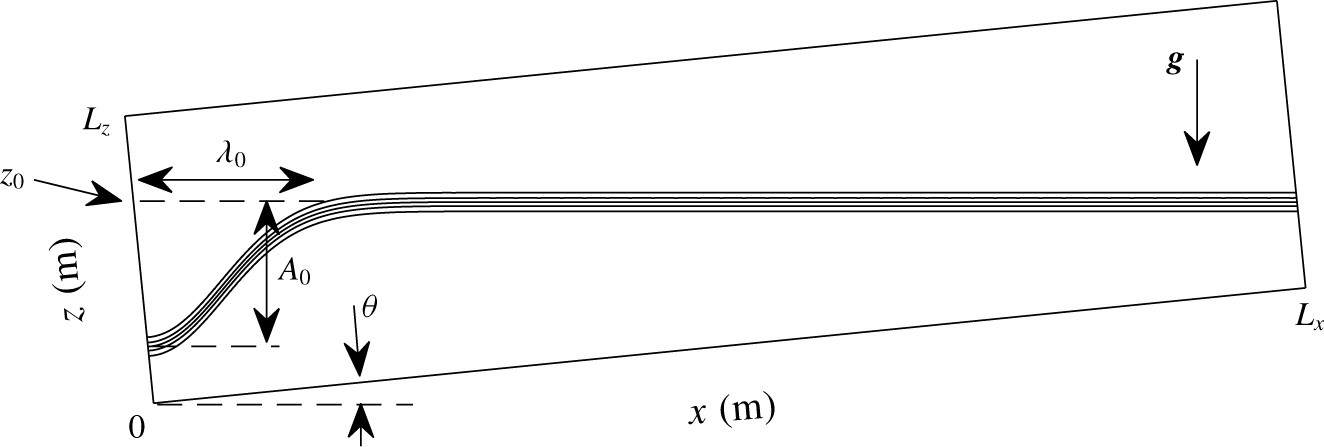
Schematic diagram of the initial density field in a tilted tank. Note that in the simulations $L_{x}\gg L_{z}$.

A schematic diagram of the model set-up is given in figure 1. The numerical simulations are performed in a rectangular tank gently tilted so the rightward end is elevated. The length and depth of the tank are labelled as $L_{x}$ and $L_{z}$, respectively. The angle between the bottom of the tank and the horizontal plane is denoted by $\unicode[STIX]{x1D703}$, while the slope of the bottom boundary is given by

(2.1)$$\begin{eqnarray}s=\tan \unicode[STIX]{x1D703}.\end{eqnarray}$$

Following this set-up, the $x$-axis is directed to the right along the tilted bottom boundary, and the $z$-axis points up along the left boundary. The tank has a rigid lid and is completely filled with fluid, so that no free surface is present.

We focus on flows in a quasi-two-layer stratification with a dimensionless density difference denoted by $\unicode[STIX]{x0394}\unicode[STIX]{x1D70C}$, which is small enough for the Boussinesq approximation to be safely adopted. The initial density profile, non-dimensionalized by the reference density $\unicode[STIX]{x1D70C}_{0}=1000~\text{kg}~\text{m}^{-3}$, is given by

(2.2)$$\begin{eqnarray}\unicode[STIX]{x1D70C}(x,z)=1-0.5\unicode[STIX]{x0394}\unicode[STIX]{x1D70C}\tanh \left\{\frac{z-z_{0}+sx+A_{0}\exp [-(x/\unicode[STIX]{x1D706}_{0})^{2}]}{d}\right\},\end{eqnarray}$$

where $z_{0}$ is the height of the undisturbed pycnocline at the left boundary, $A_{0}$ is the amplitude of the initial depression of the pycnocline at the left boundary, $\unicode[STIX]{x1D706}_{0}$ is the length of initial depression and $d$ is the half-width of the pycnocline. In all simulations, the initial velocity field is identically zero.

We emphasize that, throughout a particular experiment, the tank does not change its tilted position (as it would for an internal seiche generation experiment) so that the background state is constant. Thus, waves generated near the left boundary will shoal into shallow waters as they propagate to the right. The tilt of the upper surface means that the present set-up differs from the oceanic situation in which the upper surface (to the extent the rigid lid applies) is horizontal. However, since the evolution of the shoaling wave is controlled by the bottom boundary, which is closer to the pycnocline in the fissioning region, we believe the tilted tank is a reasonable approximation.

2.2 Governing equations

The governing equations for our time-dependent simulations are the incompressible Navier–Stokes equations under the Boussinesq and rigid-lid approximations (Kundu, Cohen & Dowling Reference Kundu, Cohen and Dowling2012), given in the tilted Cartesian coordinate system by

(2.3a)$$\begin{eqnarray}\displaystyle & \displaystyle \frac{\text{D}\boldsymbol{u}}{\text{D}t}=-\unicode[STIX]{x1D6FB}p-\unicode[STIX]{x1D70C}\boldsymbol{g}+\unicode[STIX]{x1D708}\unicode[STIX]{x1D6FB}^{2}\boldsymbol{u}, & \displaystyle\end{eqnarray}$$

(2.3b)$$\begin{eqnarray}\displaystyle & \displaystyle \unicode[STIX]{x1D735}\boldsymbol{\cdot }\boldsymbol{u}=0, & \displaystyle\end{eqnarray}$$

(2.3c)$$\begin{eqnarray}\displaystyle & \displaystyle \frac{\text{D}\unicode[STIX]{x1D70C}}{\text{D}t}=\unicode[STIX]{x1D705}\unicode[STIX]{x1D6FB}^{2}\unicode[STIX]{x1D70C}, & \displaystyle\end{eqnarray}$$

$\boldsymbol{u}$

$\unicode[STIX]{x1D70C}$

$p$

$\boldsymbol{g}$

$\unicode[STIX]{x1D708}$

$\unicode[STIX]{x1D705}$

$\boldsymbol{u}=(u,w)$

$u$

$w$

(2.4)$$\begin{eqnarray}\boldsymbol{g}=-g(\sin \unicode[STIX]{x1D703},\cos \unicode[STIX]{x1D703}).\end{eqnarray}$$

As is common practice under the Boussinesq approximation, equations (2.3) are in dimensional form, except that the density $\unicode[STIX]{x1D70C}$ and pressure $p$ are scaled by the reference density $\unicode[STIX]{x1D70C}_{0}$. Free-slip boundary conditions are applied at the left and right boundaries, while no-slip boundary conditions are applied at the top and bottom boundaries. The effect of the Earth’s rotation is neglected.

We note that variables in (2.3) are related to their counterparts in the regular, untilted Cartesian coordinate system through the rotation matrix

(2.5)$$\begin{eqnarray}\unicode[STIX]{x1D64D}(\unicode[STIX]{x1D703})=\left[\begin{array}{@{}cc@{}}\cos \unicode[STIX]{x1D703} & -\sin \unicode[STIX]{x1D703}\\ \sin \unicode[STIX]{x1D703} & \cos \unicode[STIX]{x1D703}\\ \end{array}\right].\end{eqnarray}$$

Let tilde ($\,\tilde{\,}\,$) denote variables in the untilted coordinate system. The horizontal displacement $\tilde{x}$ and vertical displacement $\tilde{z}$ can be computed as

(2.6)$$\begin{eqnarray}(\tilde{x},\tilde{z})^{\text{T}}=\unicode[STIX]{x1D64D}(x,z)^{\text{T}},\end{eqnarray}$$

while the horizontal velocity $\tilde{u}$ and vertical velocity $\tilde{w}$ can be computed as

(2.7)$$\begin{eqnarray}(\tilde{u} ,\tilde{w})^{\text{T}}=\unicode[STIX]{x1D64D}(u,w)^{\text{T}}.\end{eqnarray}$$

In the remainder of this paper, all figures are presented in the untilted coordinate system. When the angle $\unicode[STIX]{x1D703}$ is small, $\sin \unicode[STIX]{x1D703}\ll \cos \unicode[STIX]{x1D703}$ such that $(\tilde{u} ,\tilde{w})\approx (u,w)$.

2.3 Numerical method

Numerical simulations presented in this paper were performed using the numerical model described and validated in Subich, Lamb & Stastna (Reference Subich, Lamb and Stastna2013). The model employs a spectral collocation method (Trefethen Reference Trefethen2000), which yields highly accurate results. By maintaining a rectangular configuration of the entire domain, as opposed to an explicit slope region with a flat upper boundary, the scaling of the model with number of processors is nearly linear (Subich et al. Reference Subich, Lamb and Stastna2013), and allows for efficient computation even for large grid sizes. As appropriate for the boundary conditions, the Fourier sine or cosine transform is used in the along-tank direction, depending on the variable of interest, while the Chebyshev discretization is used in the direction normal to the top and bottom boundaries. The Chebyshev discretization naturally clusters grid points near the top and bottom boundaries, so that instabilities developed near the bottom boundary can be well resolved. The model employs an adaptive third-order multi-step method, where viscous and diffusive terms are solved implicitly, and pressure is computed via operator splitting.

3.1 Parameter space

Table 1.

List of simulations and their parameters. Here, $c_{lw}$ is the two-layer, linear long-wave speed, $Re$ is Reynolds number, $N_{x}$ and $N_{z}$ are the grid sizes in $x$ and $z$-directions, $\unicode[STIX]{x0394}\,x$ and $\max (\unicode[STIX]{x0394}z)$ are the horizontal and maximum vertical grid spacings, $\unicode[STIX]{x1D6FF}$ is Stokes boundary-layer thickness and $N_{bbl}$ is the number of vertical grid points within the BBL.

Numerical simulations presented in this paper are listed in table 1. For all simulations, the length and depth of the model domain are set to be $L_{x}=20~\text{m}$ and $L_{z}=0.5~\text{m}$, respectively. While these dimensions are perhaps beyond the limit of a reasonable laboratory setting, they do allow us to study the entire fissioning process over a gentle slope with $s=0.02$. To ensure that the undisturbed pycnocline intersects the left (right) boundary above (below) the mid-depth, we let $z_{0}=0.45~\text{m}$, so that the initial wave of depression will always experience a fissioning process as it shoals. Additional parameters for the initial density profile given in (2.2) are set to be $d=0.01~\text{m}$, $A_{0}=0.3~\text{m}$ and $\unicode[STIX]{x1D706}_{0}=0.35~\text{m}$, in order to ensure that the initial depression in the density profile is able to evolve into a solitary-like wave well before it reaches the turning point, and that once a solitary-like wave forms, there is no wave trailing behind it.

The Reynolds number in table 1 is defined by

(3.1)$$\begin{eqnarray}Re=\frac{c_{lw}A_{0}}{\unicode[STIX]{x1D708}},\end{eqnarray}$$

where $c_{lw}$ is the two-layer, linear long-wave speed, defined by

(3.2)$$\begin{eqnarray}c_{lw}=\sqrt{\unicode[STIX]{x0394}\unicode[STIX]{x1D70C}g\frac{h_{1}h_{2}}{h_{1}+h_{2}}},\end{eqnarray}$$

where $h_{1}$ and $h_{2}$ are the upper and lower layer thicknesses. As a rough estimate, we let

(3.3a,b)$$\begin{eqnarray}h_{1}=0.5(z_{0}+0.5L_{z})=0.35\text{ (m)}\quad \text{and}\quad h_{2}=L_{z}-h_{1}=0.15\text{ (m)}\end{eqnarray}$$

for the present model set-up, though the actual layer thicknesses vary throughout the entire domain. While Reynolds numbers reported in table 1 are on the laboratory scale, effects of Reynolds number variation will be addressed in § 3.3 in order to provide some insights on how results of our simulations might scale up to the field scale. To ensure that small-scale flow structures are properly resolved, we employ high resolution and adjust the grid sizes based on the Reynolds number. Also in table 1, the Stokes boundary-layer thickness is defined following Arthur & Fringer (Reference Arthur and Fringer2014) by

(3.4)$$\begin{eqnarray}\unicode[STIX]{x1D6FF}=2\sqrt{\frac{\unicode[STIX]{x1D708}\unicode[STIX]{x1D706}_{0}}{c_{lw}}}.\end{eqnarray}$$

We note that in the vertical direction, the Chebyshev discretization naturally clusters grid points near the bottom boundary, so that the BBL is well resolved. For all simulations, the Schmidt number, defined by

(3.5)$$\begin{eqnarray}Sc=\frac{\unicode[STIX]{x1D708}}{\unicode[STIX]{x1D705}},\end{eqnarray}$$

is fixed at $Sc=5$ by setting the diffusivity $\unicode[STIX]{x1D705}$ according to the viscosity $\unicode[STIX]{x1D708}$. The Iribarren number, defined by

(3.6)$$\begin{eqnarray}Ir=\frac{s}{\sqrt{A_{0}/\unicode[STIX]{x1D706}_{0}}},\end{eqnarray}$$

is approximately 0.02. While this value only provides a rough estimate as the wave properties change throughout the shoaling process, it is at least one order of magnitude smaller than the typical Iribarren number associated with breaking internal waves.

3.2 Base case

Figure 2.

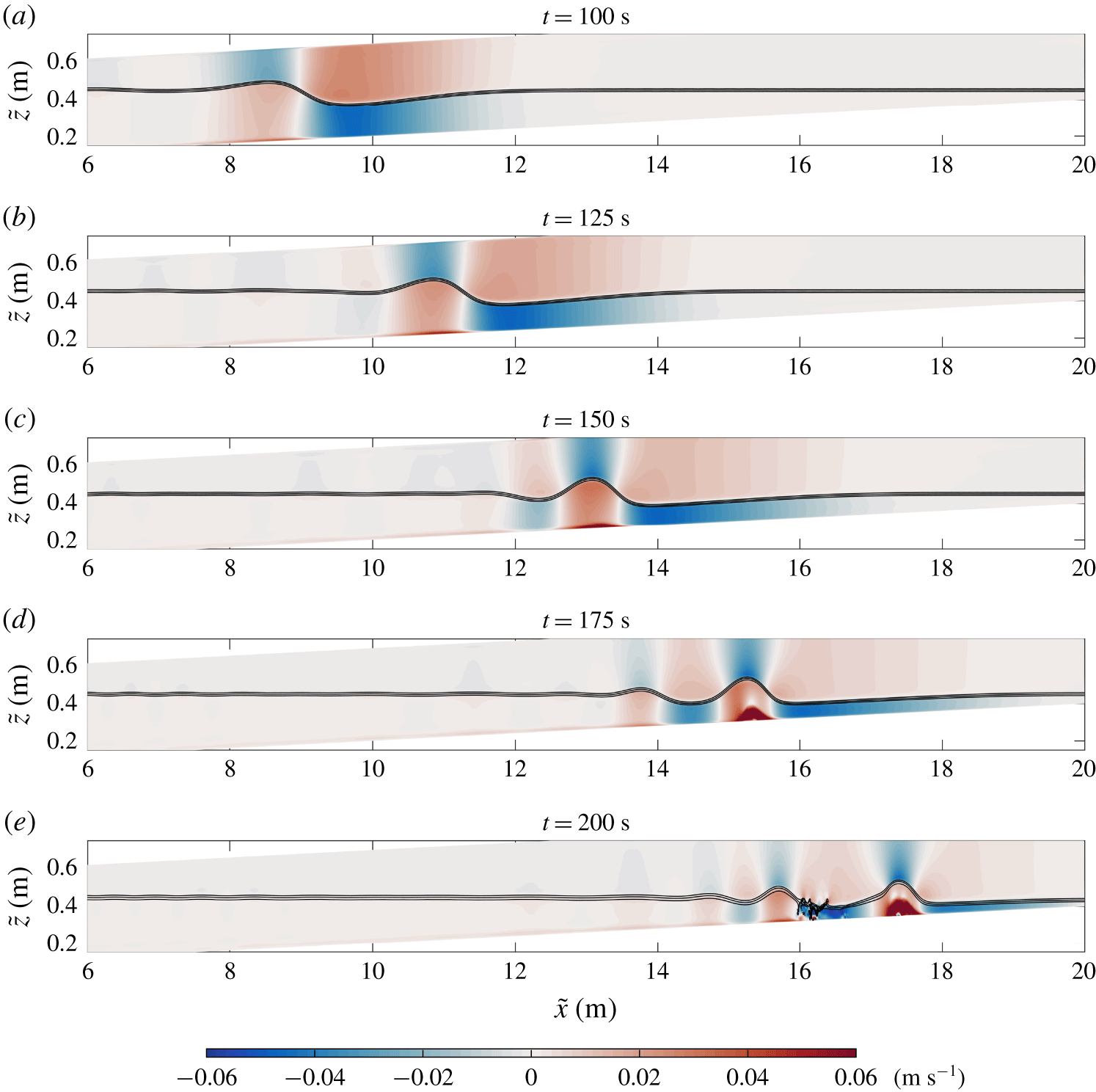
Shaded contour plots of the along-tank velocity $u$ for the ‘Base’ case from $t=100~\text{s}$ to $200~\text{s}$, showing the fissioning process of the wave and the formation of the separation bubble. Solid contours indicate the location of the pycnocline. Note that the axes are not to scale and that the maximum along-tank velocity observed at $t=200~\text{s}$ is $0.163~\text{m}~\text{s}^{-1}$.

Figure 3.

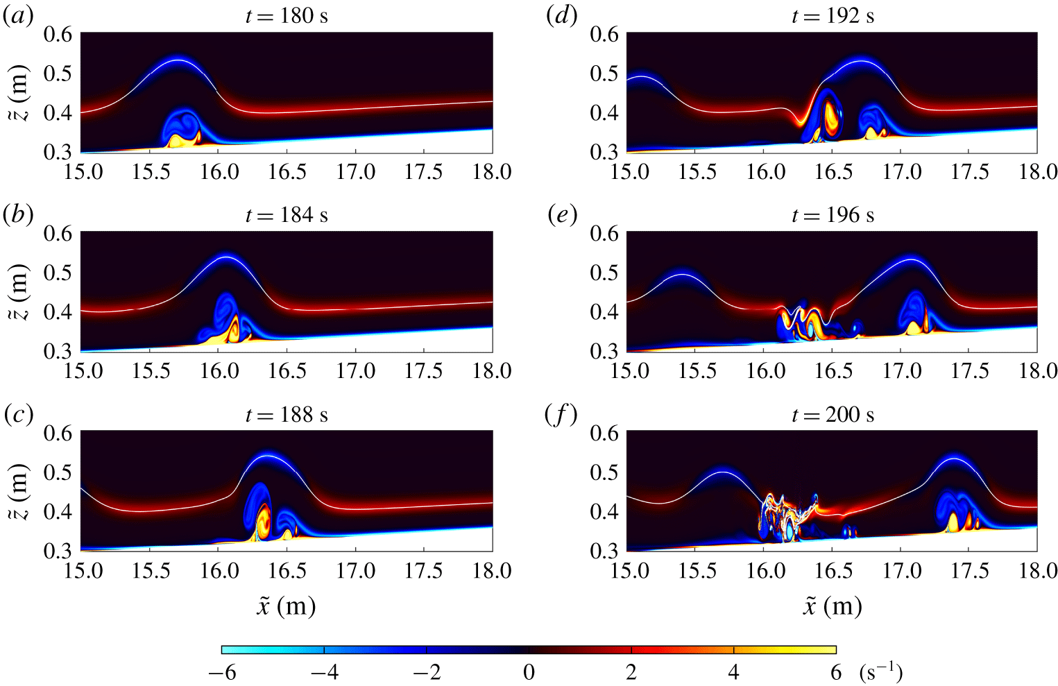
Shaded contour plots of the vorticity field $(\unicode[STIX]{x2202}u/\unicode[STIX]{x2202}z-\unicode[STIX]{x2202}w/\unicode[STIX]{x2202}x)$ for the ‘Base’ case from $t=180~\text{s}$ to $200~\text{s}$, showing the development and breakdown of the separation bubble. Solid contours indicate the location of the pycnocline.

We shall first discuss the simulation labelled as ‘Base’ in table 1. The simulation starts as an ISW of depression is generated from the initial depression of the pycnocline near the left boundary of the domain, in a process similar to the lock-release mechanism adopted in a typical laboratory setting (e.g. Carr et al. Reference Carr, Franklin, King, Davies, Grue and Dritschel2017). As the wave propagates to the right, it reaches the turning point where the pycnocline approaches the mid-depth of the domain. Beyond this point, a fissioning process occurs, where the initial wave of depression evolves into a packet of dispersive waves from which several solitary waves of elevation emerge. This process is visualized in figure 2.

The fissioning process typically occurs when the bottom slope is very gentle (usually less than or equal to 0.05) such that nonlinear steepening is insufficient to cause wave overturning (Aghsaee et al. Reference Aghsaee, Boegman and Lamb2010). For this reason, it is generally believed that the fissioning process does not give rise to significant turbulent mixing and hence does not contribute to cross-boundary-layer transport. Nevertheless, this is not the case in our simulation, as boundary-layer instability in the form of a separation bubble can be clearly observed in figure 2. The separation bubble is evident in all panels and can thus be thought of as originating in the lee of the leading wave of depression as it steepens at the back during shoaling. By $t=150~\text{s}$ (panel c), the leading wave of depression is quite small in amplitude and extremely broad. Thus, the developing wave of elevation can be interpreted as the primary wave, and the separation bubble can be seen to fill the footprint of this wave and propagate with the wave. Indeed, as the wave of elevation decreases in length in panels (d) and (e), the separation bubble can be seen to shorten as well and begin to roll up. The secondary wave appears to develop its own separation bubble, though this is only clear in panel (e), due to the clear alternation of red and blue regions in the BBL region.

Details of the development and breakdown of the separation bubble can be visualized from the vorticity plots shown in figure 3. The figure suggests that vorticity associated with the jet near the bottom boundary induces strong vorticity above the BBL and leads to roll-up of the vorticity in the wave footprint. As the wave propagates and shoals, the separation bubble develops gradually and eventually breaks down into two parts. One of them is trapped beneath the wave and keeps propagating with it, while the other is shed behind the leading wave and interacts with the trailing waves.

It has been shown in past literature that a necessary condition for the formation of a separation bubble in a wave of elevation is the presence of a background current oriented against the direction of wave propagation (see, e.g. figure 6 of Boegman & Stastna Reference Boegman and Stastna2019). In our simulation, while the amplitude of the leading wave of depression diminishes after the fissioning process, the current induced by it persists, meaning that its wave energy is not fully transferred into the packet of trailing waves of elevation. Thus, even after the fissioning process, the leading wave of depression is able to induce an adverse pressure and a current oriented against the direction of wave propagation. This current essentially plays the role of a background current and triggers the boundary-layer instability upon interaction with the leading wave of elevation. We note that the point of view of treating leading, long waves as setting a background state for trailing waves was used successfully in Lamb & Warn-Varnas (Reference Lamb and Warn-Varnas2015) to study the shoaling of ISW over complex bathymetry in the South China Sea.

Figure 4.

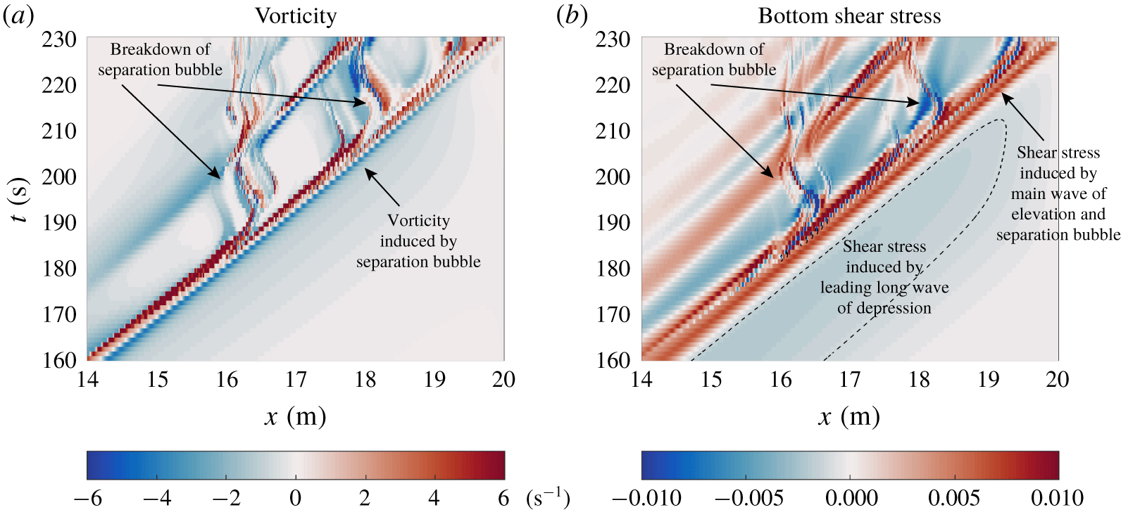
Hovmöller plots of (a) vorticity $(\unicode[STIX]{x2202}u/\unicode[STIX]{x2202}z-\unicode[STIX]{x2202}w/\unicode[STIX]{x2202}x)$ in a layer 0.01 m above the bottom boundary and (b) bottom shear stress $\unicode[STIX]{x1D70F}$, for the ‘Base’ case from $t=160~\text{s}$ to 230 s.

To examine the details of the boundary-layer dynamics induced by the evolution of the separation bubble, we calculate (a) the vorticity in a layer 0.01 m above the bottom boundary and (b) the shear stress along the flat bottom boundary $z=0$. The latter, when scaled by the dynamic estimate $0.5\unicode[STIX]{x1D70C}_{0}c_{lw}^{2}$, is defined as

(3.7)$$\begin{eqnarray}\unicode[STIX]{x1D70F}(x)=\frac{2\unicode[STIX]{x1D708}}{c_{lw}^{2}}\frac{\unicode[STIX]{x2202}u}{\unicode[STIX]{x2202}z}.\end{eqnarray}$$

The results are shown as Hovmöller plots for the late stage of the fissioning process in figure 4. We note that the grainy nature of these and similar plots is not due to a reduced resolution in either space or time, but due to the fact that the numerical model only saves the full fields with a fixed frequency. In this figure, the strong near-bottom vorticity and bottom shear stress in the diagonal direction is associated with the passage of the main wave of elevation, in which the separation bubble develops near the BBL as the wave propagates. The two breakdown events of the separation bubble can be clearly seen, as indicated in the figure. Behind the main wave of elevation, vorticity and bottom shear stress due to the separation bubble are both as strong as those due to the wave itself. These observations imply that the development and breakdown of the separation bubble can provide an effective mechanism for significant cross-boundary-layer transport and possibly sediment resuspension (though this last point requires a proper accounting for the sediment).

We note that while simulation with free-slip bottom boundary conditions has also been performed (not shown here), the formation of a separation bubble is not observed. This means that when simulating the fissioning process, the presence of a no-slip bottom boundary is a necessary condition for both the onset of boundary-layer instability and any eventual overturning that results from it.

3.3 Reynolds number variation

Figure 5.

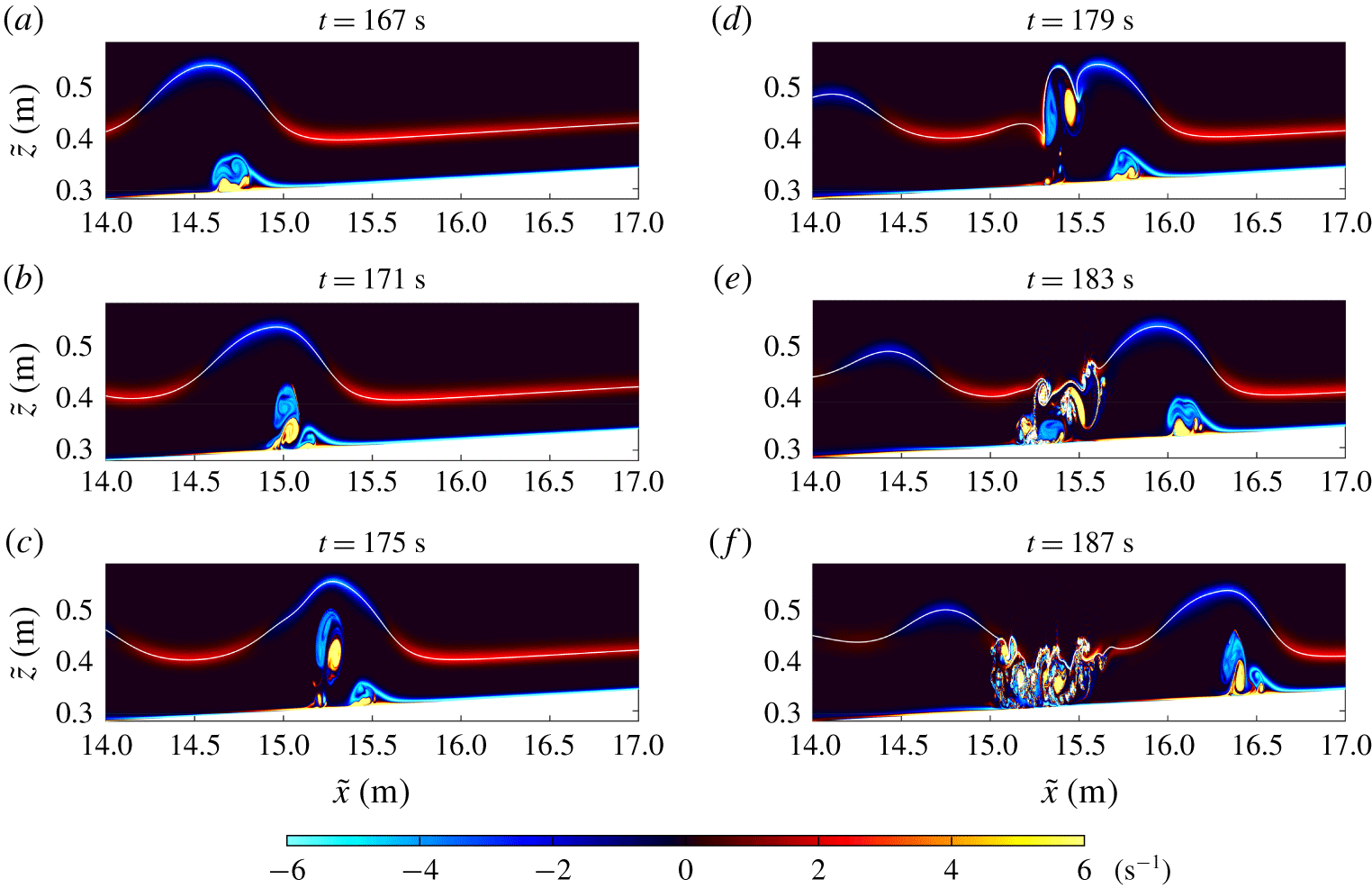
Same as figure 3 but for the ‘Low $\unicode[STIX]{x1D708}$’ case from $t=167~\text{s}$ to $187~\text{s}$. The Reynolds number of this case is doubled from that of the ‘Base’ case.

To test the effect of a varying Reynolds number, we performed three additional experiments (only the results for one are shown). In the ‘Low $\unicode[STIX]{x1D708}$’ case, we increase the Reynolds number by decreasing the viscosity $\unicode[STIX]{x1D708}$, whereas in the ‘Faster’ case, we increase the Reynolds number by increasing the density difference $\unicode[STIX]{x0394}\unicode[STIX]{x1D70C}$, which then leads to an increase in the velocity scale $c_{lw}$. In the ‘Half $Re$’ case, we halve the Reynolds number by doubling the viscosity $\unicode[STIX]{x1D708}$.

For the ‘Low $\unicode[STIX]{x1D708}$’ case, the early stage of the fissioning process is not shown as the leading wave of depression and main wave of elevation behave similarly to those of the base case. In the late stage when the boundary-layer interaction occurs, however, the separation bubble develops faster and breaks down earlier, as suggested by figure 5. Comparison of figures 3 and 5 suggests that strength of the vorticity induced by the boundary-layer instability increases as the Reynolds number increases. Consequently, the overall flow is more likely to be turbulent, and the cross-boundary-layer transport also occurs earlier and tends to be stronger. A small separation bubble can be seen in the footprint of the second wave of elevation in panel (f). It is clear that in the higher Reynolds number case the dynamics of this separation bubble will be swamped by the vorticity associated with material ejected from the leading wave.

Figure 6.

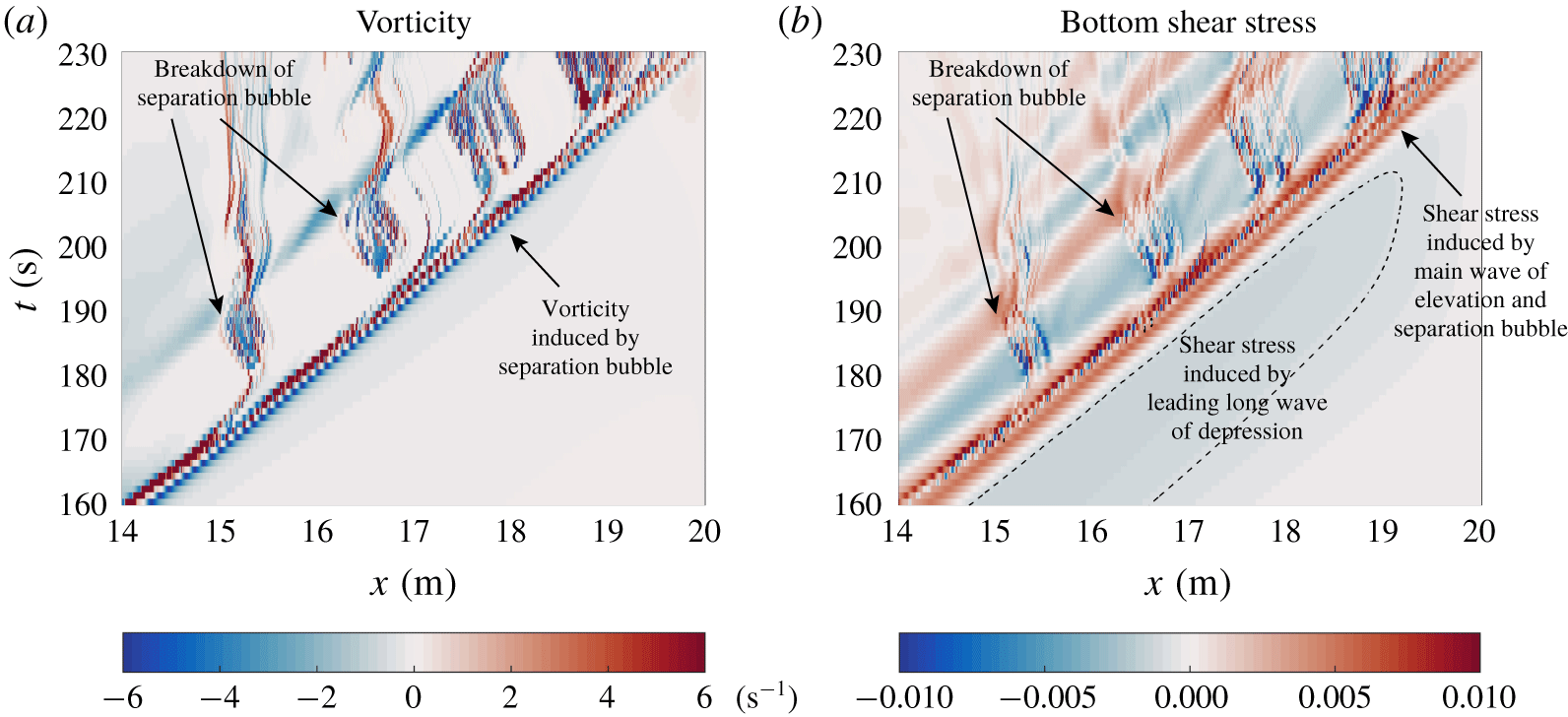
Same as figure 4 but for the ‘Low $\unicode[STIX]{x1D708}$’ case from $t=160~\text{s}$ to 230 s.

Figure 6 shows that a higher Reynolds number leads to stronger near-bottom vorticity and bottom shear stress. In particular, four breakdown events of the separation bubble can be seen before the main wave of elevation reaches the end of the tank, whereas in the base case only two are visible.

The ‘Faster’ case is not shown here as the overall flow behaves very similar to that in the ‘Low $\unicode[STIX]{x1D708}$’ case, except that the characteristic velocity scale is twice as large as that in the ‘Low $\unicode[STIX]{x1D708}$’ case. This means that the observed effect of a higher Reynolds number, namely a stronger cross-BBL transport, is robust. With a much higher Reynolds number on the field scale, the implication is that fissioning over gentle slopes provides a means for turbulent mixing and cross-BBL transport that is comparable in efficiency when compared to wave breaking over steeper slopes.

We have also performed another simulation, labelled as ‘Half $Re$’ in table 1, to examine the effect when the Reynolds number is reduced from the base case. Although the results are not shown here, the primary observation is that the separation bubble is confined within the main wave of elevation until it reaches the right boundary, and that the breakdown of separation bubble does not occur throughout the shoaling process.