1. Introduction

In many scientific fields phenomena are explained or predicted by pointing at their underlying mechanisms. Such mechanisms are thought of as concrete entities located at specific regions in space-time that produce the respective phenomena. They are characterized by formulations like this: “A mechanism underlying a behavior is a complex system which produces that behavior by the interaction of a number of parts according to direct causal laws” (Glennan Reference Glennan1996, 52). For alternative formulations, see, for example, Machamer, Darden, and Craver (Reference Machamer, Darden and Craver2000, 3), Bechtel and Abrahamsen (Reference Bechtel and Abrahamsen2005, 423), and Illari and Williamson (Reference Illari and Williamson2012, 120).

According to mechanists, mechanisms are dynamic causal systems; they are wholes consisting of several spatiotemporally arranged and interacting parts producing certain behavior. Besides having these properties, mechanisms are oftentimes (but not always) self-regulating systems including a lot of feedback loops. Typically (but not necessarily), they are also hierarchically organized (i.e., they consist of several interacting submechanisms that may themselves be built up of submechanisms, etc.). The more is known about the structure of these submechanisms, the more accurate the predictions of the phenomena these mechanisms bring about will typically be.

Although characterizations, like the one formulated by Glennan (Reference Glennan1996) above, are intuitively quite clear, they are not as helpful as one may hope for when it comes to quantitatively precise explanations/predictions of phenomena of interest. This deficit can easily be seen by means of the following example: the question of why a car speeds up when the gas pedal is pressed can be answered by pointing at/describing the underlying mechanism (i.e., the motor and how it is connected to the gas pedal, the wheels, the gas tank, etc.), but questions including numerical details like why the acceleration of the car is a when the gas pedal is pressed with pressure p cannot be answered that easily. The answer to a question like the latter requires a formalism capable of capturing/computing the numerical details/effects of specific manipulations of said mechanism.

Such a formalism must be able to represent the above-mentioned characteristic properties of mechanisms in an adequate way. Casini et al. (Reference Casini, Illari, Russo and Williamson2011) propose to model mechanisms on the basis of so-called recursive Bayesian networks, which were originally developed by Williamson and Gabbay (Reference Williamson, Gabbay and Gillies2005) to model nested causal relationships. In doing so they focus on an adequate representation of the hierarchical structure of mechanisms and represent submechanisms by means of a recursive Bayesian network’s vertices. I will briefly introduce the formal preliminaries needed to take a closer look at their approach and explain their account on a very simple exemplary toy mechanism in section 2. In section 3 I will highlight two problems with Casini et al.’s approach: their approach (i) does not allow for a graphical representation of how a mechanism’s macrovariables are causally connected to the mechanism’s causal microstructure, which is essential when it comes to mechanistic explanation, and it (ii) leads to the fatal consequence that a mechanism’s macrovariables’ values cannot be changed by any intervention on the mechanism’s microstructure whatsoever and, thus, contradicts the fact that scientists regularly perform so-called bottom-up experiments to investigate which are the mechanism’s constitutively relevant parts. In section 4 I present an alternative approach for modeling nested mechanisms: submechanisms should not be represented by means of a causal graph’s vertices, like in Casini et al.’s approach, but rather by means of a causal graph’s edges. I finally demonstrate using the above-mentioned exemplary mechanism that this approach does not fall prey to problems (i) and (ii).

2. Bayesian Networks, Recursive Bayesian Networks, and the Recursive Bayesian Network Approach

A Bayesian network (BN) is a triple that satisfies the so-called Markov condition (MC). Graph is a graph whose vertices (i.e., the elements of V) are random variables that may take a number of different values, while E is a binary relation on V . Relation E’s elements are called edges and can be graphically represented via different kinds of lines or arrows in G. A BN’s associated graph is always a directed acyclic graph (DAG), that is, a graph whose edges are arrows () and that does not contain a substructure of the form . And P is a joint probability distribution over the random variables in V.

In this definition ‘Des(X)’ stands for the descendants (i.e., the successors) of X in graph , ‘Par(X)’ for the parents (i.e., the direct predecessors) of X in graph , and ‘’ for probabilistic independence of X and Y conditional on Z (i.e., for all X-, Y-, and Z-values x, y, and z, respectively, provided ). BNs can be causally interpreted; that is, they can be understood as a certain type of causal model. When doing so, a BN’s associated graph G represents the system of interest’s causal structure: ‘’ in such a causal graph G stands for ‘X is a direct cause of Y in G’, and a chain of (one or more) arrows (i.e., a directed path) going from X to Y stands for ‘X is a (direct/indirect) cause of Y in G’. A structure of the form is called a common cause path between X and Y.

When one uses BNs for causal modeling, MC is causally interpreted also. Under its causal interpretation, MC becomes the so-called causal Markov condition (CMC) that is satisfied by a causal model if and only if every is probabilistically independent of all its noneffects conditional on its direct causes (cf. Spirtes et al. Reference Spirtes, Glymour and Scheines2000, 29).Footnote ¹

The graph of a BN satisfying MC/CMC determines the following Markov factorization:Footnote ²

A recursive Bayesian network (RBN) is a BN in which the values of variables in V can be BNs themselves. Such variables are called network variables, while variables that do not have BNs as values are called simple variables. Casini et al. (Reference Casini, Illari, Russo and Williamson2011) suggest to represent a mechanism by an RBN and a submechanism by a network variable whose values are BNs representing the possible states of this submechanism. They propose, in addition to the causal interpretation of MC, an additional modeling assumption, the recursive causal Markov condition (RCMC):

Set is the set of noninferiors or descendants of X, that is, the set of random variables that are neither inferiors nor descendants of X. The inferiors of X are the variables of a lower-level BN representing states of the submechanism described by X at the higher level, the variables of the lower-level BNs representing states of submechanisms of this submechanism, and so on. Set is the set of direct superiors of X and contains those variables of the next-level-up BN representing a submechanism whose states are described by lower-level BNs including X. (For an illustration of these notions, see the water dispenser example introduced below.) Casini et al. (Reference Casini, Illari, Russo and Williamson2011, sec. 4) suggest interpreting the inferiority/superiority relation as constitutive relevance in the sense of Craver (Reference Craver2007a, Reference Craver2007b).

Let me now briefly explain how probabilistic interlevel explanation/prediction works in Casini et al.’s (Reference Casini, Illari, Russo and Williamson2011) RBN approach. One therefore needs to define as the RBN ’s variable set V under the transitive closure of the inferiority relation.Footnote ³ Let be the set of network variables in . Then for every instantiation of network variables in , a simple BN can be constructed: the flattening of the RBN with regard to . The nodes of this new BN are the simple variables in together with the instantiations of the network variables in . BN ’s set of edges contains an arrow pointing from X to Y if and only if X is a parent or direct superior of Y in the RBN, and ’s probability distribution is determined by the following equation:

where X_jl are the direct superiors of X_i.

The flattenings of an RBN determine a unique probability distribution over that allows for quantitative reasoning across the diverse levels of the mechanism represented by the RBN:Footnote ⁴

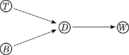
Let me now briefly illustrate how the modeling approach proposed by Casini et al. (Reference Casini, Illari, Russo and Williamson2011) works on a very simple toy example, that is, the water dispenser mechanism. This device normally dispenses cold water and water close to the room temperature when its tempering button is pressed. The water dispenser can be represented by an RBN whose top-level graph is depicted in figure 1.

Figure 1.

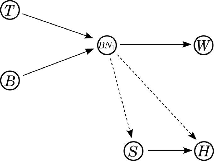
Variable T represents the room temperature, stands for whether the tempering button is pressed or not, W stands for the temperature of the water dispensed, and D is a network variable that represents a submechanism, that is, the water dispenser’s water temperature regulation unit. This regulation unit consists of two lower-level parts: a temperature sensor (S) and a heater (H). Variable D has two possible values: BN ₁ (water temperature is regulated, and thus, one gets water close to the room temperature) and BN ₀ (water temperature is not regulated, and cold water is dispensed as a result). Values BN ₁ and BN ₀ are two BNs with the same topological structure (depicted in fig. 2) but with different associated probability distributions. If , then the heater is working on a level corresponding to the input of the temperature sensor. If , then H is probabilistically insensitive to S. Note that the singleton of D is the set of direct superiors of S and H () in our exemplary mechanism, while is the set of inferiors of .

Figure 2.

When one wants to use the RBN approach for probabilistic predictions across the levels of a mechanism, one first has to construct the RBN’s flattenings as described above. Figure 3 shows the flattening of the RBN with regard to . Note that the two interlevel arrows from D to S and from D to H stand for the direct superiority/inferiority relation and should not be causally interpreted:Footnote ⁵ S and H are not effects of D; they rather stand for constitutively relevant parts of the submechanism represented by D. To indicate this fact, the arrows are dashed in figure 3.

Figure 3.

According to equation (2), the conditional probability distribution of this flattening is , , , , , . The conditional probability distribution of the flattening of the RBN with regard to is , , , , , . According to equation (3), the two flattenings of the RBN determine a joint probability distribution over ; that is, , where the probabilities on the right-hand side of the equation are determined by the flattening induced by T, B, D, W, S, H. This probability distribution can be used for quantitative prediction across the two levels of our exemplary mechanism.

3. Two Problems with the RBN Approach

Let me now expose the two deficits of the RBN approach announced in section 1. Problem (i): while RBNs clearly allow for quantitative reasoning across the diverse levels of mechanisms, they do not tell us how exactly submechanisms are causally connected to their mechanisms. In case of the water dispenser example, for instance, the RBN’s graph tells us neither how T and B causally influence S and H nor how S and H are causally relevant for W; that is, there are no arrows between those variables in the RBN’s graph, and it is unclear over which causal paths probabilistic influence from T and B is propagated through the mechanism’s microstructure to W. But is the graphical representation of such causal information required at all? Is it not sufficient that the RBN captures the probabilistic dependencies between the variables in ? The answer to the latter question is no. One of the reasons for this is simply that mechanistic explanation requires information about how exactly (i.e., over which causal pathways) certain inputs to the system influence the mechanism’s microstructure and how changes in this microstructure bring about the phenomenon (or phenomena) of interest at the macrolevel (cf., e.g., Bechtel Reference Bechtel, Shouten and de Jong2007, sec. 3).Footnote ⁶ In causal models this information is typically provided by the model’s associated probability distribution together with its graph’s topology. Illustrated in our example: if our RBN model adequately represents the water dispenser mechanism, then the information that the tempering button is not pressed () will screen W off from T. (The room temperature is only relevant for the temperature of the water dispensed when the tempering button is pressed.) The RBN’s associated probability distribution may give us the correct probabilistic dependencies/independencies, but its graph does not provide the causal information to mechanistically explain this probabilistic behavior. So the model does not tell us that the probabilistic influence of T on W breaks down because fixes the value of H and because H lies on the only directed causal path from T to W.

The representation of such causal information in the model’s graph is important not only for mechanistic explanation but also when it comes to questions of manipulation and control. (Purely probabilistic models cannot distinguish between observation and manipulation; cf. Pearl Reference Pearl2009, sec. 1.3.1.) So how, for example, could we intervene on the mechanism’s microstructure in such a way that we can amplify or decrease certain external influences? If we want, for instance, to increase or decrease T’s causal effect on W in our exemplary mechanism, then the information (which is not captured by the RBN’s graph) that S lies on a causal path from T to W is crucial. Such knowledge tells us that we can increase/decrease T’s effect on W by manipulating S in certain ways, for example, by putting an additional heat source to the sensor S or by cooling S.Footnote ⁷

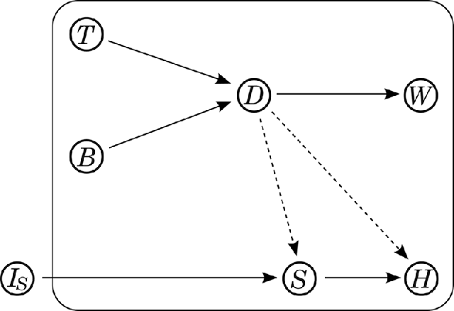
Let me now illustrate problem (ii), which is presumably the more striking one of the two problems for the RBN approach: recall that the probability distribution that allows for probabilistic reasoning across all levels of a mechanism is constructed via the flattenings of the RBN (see sec. 2). For our exemplary mechanism this probability distribution would be , where the probabilities on the right-hand side of the equation are determined by the flattening induced by T, B, D, W, S, H. This probability distribution can be captured by a BN with a graph like the one depicted in the box in figure 4. (Again, the continuous lines could, while the dashed ones should not, be causally interpreted.) Now assume that one would, for example, intervene on S by means of an intervention variable I_S. Such an intervention on S would—and this can directly be read off the BN’s associated graph’s topology (depicted in fig. 4)—not have any probabilistic influence on any macrovariable at all.

Figure 4.

So, according to the RBN approach, intervening on a mechanism’s microvariables does not have any probabilistic influence on any one of the macrovariables whatsoever. This does not only contradict what we observe when looking at the (bottom-up) experiments scientists perform. It is also inconsistent with one of the core features of mechanisms: a mechanism’s macro- and its constitutively relevant microbehaviors should be mutually manipulable (cf. Craver Reference Craver2007a, Reference Craver2007b). Note that the inferiority relation is explicitly intended to represent constitutive relevance within the RBN approach (cf. Casini et al. Reference Casini, Illari, Russo and Williamson2011, sec. 4).

4. An Alternative

Let me now propose an alternative to Casini et al.’s (Reference Casini, Illari, Russo and Williamson2011) method for representing nested mechanisms. Instead of BNs I use causal models whose graphs are not restricted like those of BNs. In particular, the causal graphs I use can contain two kinds of edges: , which means that X is a direct cause of Y in the graph, and , which means that X and Y are effects of a latent common cause, that is, a cause of X and Y not represented within the graph’s variable set V.Footnote ⁸ Contrary to Casini et al., I suggest to represent mechanisms not by means of variables but by means of causal arrows. So the simplest representation of a mechanism’s top level would be a causal model with graphical structure or . In the first case, X would be the mechanism’s input, Y its output, and the arrow ‘→’ would stand for the (not further specified) mechanism at work. In the latter case, X and Y would both represent different outputs produced by one or more not-further-specified (and maybe yet unknown) common causes. Also here, ‘↔’ would stand for the mechanism at work.

To represent the mechanism’s causal microstructure, one can now assign a second causal model to the top-level causal model that specifies how exactly probabilistic influence between X and Y is propagated through the mechanism’s causal microstructure. Both causal models must fit together with respect to the causal information contained in their associated graphs as well as with respect to the probabilistic information stored in their associated probability distributions. This is guaranteed by the following notion of a restriction of a causal model. This notion is basically a slightly modified version of Steel’s (Reference Steel2005, 11) notion of a restricted graph complemented by conditions for bidirected arrows:

Definition 3 determines for every causal model and for every proper subset V of a unique restriction . This restriction is called ’s restriction to V. The introduced notion of a restriction allows for marginalizing out variables in such a way that the causal as well as the probabilistic information captured by the restricted model is preserved: can be interpreted as a higher- and as a lower-level mechanism’s causal structure in definition 3. Condition a guarantees that the higher-level structure contains fewer variables than the lower-level one, b ensures that ’s and ’s probability distributions fit together, and c that also their associated causal structures do. Thanks to c1 all components of a mechanism represented at both levels are directly causally connected at the higher level whenever they are directly causally connected at the lower level, so no direct causal connection between two variables represented at both levels gets lost when going from the lower to the higher level. In addition it guarantees that there is a direct causal connection for every directed causal path in the lower-level structure whose intermediate components are not represented at the higher-level model’s associated graph. Condition c2 tells us when we have to draw a bidirected edge (↔) between two variables X and Y in the higher-level model’s graph: draw such a bidirected edge whenever there also is one at the lower level, if all variables on a common cause path of X and Y are marginalized out when going from the lower- to the higher-level structure or when all variables lying on a path at the lower level that indicates a latent common cause of X and Y are marginalized out.Footnote ¹¹ Condition d prevents causal connections at the higher level that do not have a counterpart at the lower level. Figure 5 illustrates how marginalizing out variables functions according to definition 3, by showing an exemplary causal structure and some of its possible restrictions.

Figure 5.

According to definition 3, the graph of the restriction of a causal model with the graph depicted above would be , if one chooses to marginalize out U. It would be , if marginalizing out Z, and , if marginalizing out Z and U. When one restricts the original model to , the resulting structure would be (without an edge between X and Z).

Let me now further develop the above-mentioned idea of representing nested mechanisms by edges instead of vertices. For this purpose I introduce the following notion of a multilevel causal model (MLCM) that is based on the definition of a restriction (definition 3). I propose MLCMs as adequate means for representing the hierarchical organization of mechanisms (below I will demonstrate that MLCMs do not fall prey to the two problems of the RBN approach discussed in sec. 3):

According to definition 4, an MLCM is an n-tuple consisting of several causal models (condition a) that are intended to represent causal structures at different levels. According to b, every causal model M_i in the ordering different from M ₁ is a restriction of the first causal model M ₁, so M ₁ stands for the mechanism’s lowest level, while every M_i different from M ₁ represents one of its higher levels. Condition c captures a basic assumption of the causal nets approach; that is, that every robust probability distribution is produced (and, thus, can be explained) by some underlying causal model satisfying CMC (cf. Spirtes et al. Reference Spirtes, Glymour and Scheines2000, 124–25). So an MLCM of a mechanism is complete only when all probabilistic dependencies of any higher-level model can be explained by a lowest-level causal model M ₁ that satisfies CMC.

Definition 4 does not directly tell us much about the hierarchical organization of the mechanism and its submechanisms represented by the MLCM’s causal models; it just tells us that M ₁ stands for the lowest level. Fortunately, a unique level graph can be constructed for every MLCM. Such a level graph is a kind of metagraph that provides exactly the information requested above: information about the hierarchical relation of nested mechanisms represented by the MLCM:

According to a, a level graph is a graph over the causal models of an MLCM. Condition b instructs one to draw a directed edge from one of these to another whenever V_i is a proper subset of V_j and there is no in V such that V_k is a proper subset of V_j and a proper superset of V_i. So the directed paths in a level graph correspond to the set-theoretical proper subset relation (i.e., in G if and only if ). Because every causal model of the MLCM different from is a restriction of M ₁, the vertex set V_i of every such model M_i is a proper subset of V ₁. So the level graph G will be a DAG containing only one vertex with no exiting arrows (i.e., ), while there will be a directed path from every M_i different from M ₁ to M ₁.

Now some information about the hierarchical organization of causal models of an MLCM can be read off this MLCM’s level graph G: whenever there is a directed path from M_i to M_j in the level graph G, then M_i represents a higher-level causal structure than M_j does. And whenever a causal model lies on such a directed path from M_i to M_j, then M_k represents a causal structure on a level between M_i and M_j. So what we basically get by drawing a level graph is a strict order among causal models of an MLCM.

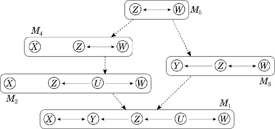
Let me now illustrate the MLCM approach for modeling mechanisms by an abstract example. Figure 6 shows the causal structures of the causal models of an MLCM plus the MLCM’s level graph that connects these models and provides information about the hierarchical order of the mechanism’s levels the MLCM represents. The lowest-level causal model M ₁’s graph is . One gets the higher-level model M ₂ with graph by marginalizing out Y, and the higher-level model M ₃ with graph by marginalizing out X and U. Note that the MLCM’s level graph does not provide any information about whether these two models (i.e., M ₂ and M ₃) represent structures at the same or at different levels of organization. By marginalizing out U from M ₂, one arrives at the higher-level causal model M ₄ with structure . Note that the formalism again does not provide any information about whether M ₄ represents a mechanism at the same level as the one represented by M ₃. One can further restrict M ₃ and M ₄ to M ₅, with causal graph . Model M ₅ describes the represented mechanism at the top level. Note that the MLCM’s level graph tells us that causal models M ₂, M ₃, and M ₄ describe the mechanism’s causal structure on levels between the mechanism’s top and its lowest level represented by M ₅ and M ₁, respectively.

Figure 6.

Boxed graphs are the associated causal graphs of an MLCM’s causal models . Dashed lines are the edges of this MLCM’s level graph.

As a last step, I will demonstrate using our exemplary mechanism introduced in section 2 (i.e., the water dispenser) that MLCMs do not share problems (i) and (ii), which Casini et al.’s (Reference Casini, Illari, Russo and Williamson2011) RBN approach has to face, and that MLCMs nicely capture another important feature of nested mechanisms: as long as the details of a mechanism are not considered, the same input should lead to the same output on all of the mechanism’s levels.

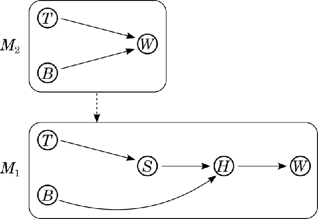
The water dispenser mechanism can be represented by an MLCM , where the graph in the upper box in figure 7 shows M ₂’s and the one in the lower box shows M ₁’s causal structure. Model M ₁ represents the water dispenser’s submechanism, that is, the water temperature regulation unit, and how it is causally connected to the mechanism’s macrovariables. Note that this submechanism is not represented by a variable like in Casini et al.’s (Reference Casini, Illari, Russo and Williamson2011) RBN approach but by M ₂’s graph at the higher level. Variables T and B are this submechanism’s input variables; W is its output variable. The MLCM ’s level graph is . When we go from M ₂ to M ₁, we zoom into the microstructure of the submechanism represented by at the top level. Since M ₂ is a restriction of M ₁ in the MLCM, it follows from definition 3b that holds for arbitrarily chosen W-, T-, and B-values w, t, and b, respectively. So as long as only the variables contained in both causal models’ variable sets are considered, the same input will lead to the same output at both levels, and thus, MLCM captures the aforementioned feature of nested mechanisms.

Figure 7.

Water dispenser mechanism by means of a two-stage MLCM (causal models M ₁ and M ₂). Graph with the dashed edge connecting the MLCM’s two causal models M ₁ and M ₂ is the MLCM’s level graph.

Since the causal arrows in M ₁ tell us exactly how the submechanism’s components S and H are causally connected to the rest of the mechanism (i.e., T, B, and W), the MLCM representation captures property (i): the MLCM can graphically represent the causal connections between the represented mechanism’s macro- and microvariables. This gives us causal information that is crucial for questions concerning explanation, manipulation, and control. It tells us why certain inputs (i.e., conditionalizing on certain T- and B-values) bring about (or explain) certain outputs (i.e., probabilities of certain W-values): T is directly causally relevant for S, B and S are direct causes of H, and H is the only direct cause of W in our toy mechanism. This causal information does tell us, for example, why T’s probabilistic influence on W breaks down when . It is because the only productive causal path from T to W goes through H. Variable fixes H’s value and, thus, probability propagation between T and W along this path is blocked when H’s value is fixed. It also tells us that T’s influence on W can be amplified or decreased by manipulating S or H by means of soft interventions, while B’s effect on W can only be modified by changing H’s behavior. The MLCM can also capture property (ii): intervening on the mechanism’s microstructure (i.e., on S or H) will typically have a probabilistic influence on the mechanism’s macrobehavior (i.e., on certain W-values).

Like Casini et al.’s (Reference Casini, Illari, Russo and Williamson2011) RBN approach, the MLCM representation provides a unique probability distribution over the set of all variables appearing in the causal models of the MLCM. Since the first causal model in an MLCM’s ordering also contains all variables of the causal models M_i appearing later in that particular ordering, said unique probability distribution is M ₁’s probability distribution P ₁. When it comes to quantitative prediction, one can, thanks to the fact that every causal model appearing later in the ordering is a restriction of M ₁, just choose one of the causal models in the MLCM that contains all the variables of interest and then compute the probabilities for the phenomena of interest accordingly.

5. Conclusion

In this article I tackled the question of how mechanisms, and especially their hierarchical organization, can be represented within a causal graph framework. In section 2 I discussed an approach for modeling such nested mechanisms proposed by Casini et al. (Reference Casini, Illari, Russo and Williamson2011). I introduced Bayesian networks and recursive Bayesian networks and explained how they can be used for causal modeling. I then illustrated Casini et al.’s RBN approach, which suggests representing submechanisms by network variables of an RBN, by means of a very simple toy example, that is, the water dispenser mechanism. In section 3 I illustrated two problems with the RBN approach by means of the exemplary mechanism introduced in section 2: (i) an RBN does not graphically encode information about how a mechanism’s submechanisms are causally connected to the rest of this mechanism. Such information is, however, relevant when it comes to questions of mechanistic explanation, manipulation, and control. (ii) It follows from the RBN approach that intervening on some of a mechanism’s microvariables cannot have any probabilistic influence on some of this mechanism’s macrobehavior whatsoever. This consequence stands in stark contrast to scientific practice; scientists typically carry out so-called bottom-up experiments to distinguish between a mechanism’s constitutively relevant and its irrelevant parts. In section 4 I developed an alternative modeling approach for nested mechanism: the MLCM approach. This approach represents submechanisms not by means of a causal model’s variables but by the edges of its associated graph. I finally demonstrated, again using the exemplary mechanism of the water dispenser, that the MLCM approach does not fall prey to problems (i) and (ii), which Casini et al.’s RBN approach has to face.