

1. Introduction
Prevalence is a measure of disease frequency that focuses on existing status rather than new events (Rothman and Greenland, Reference Rothman, Greenland, Rothman and Greenland1998). Though incidence is of primary importance in etiological research, prevalence is often used in the study of chronic diseases of insidious onset (e.g. Johne's disease) where incident cases are difficult to define even if populations are monitored longitudinally.
Diagnostic tests are commonly used for prevalence surveys and, ideally, true prevalence should be estimated from apparent (test) prevalence by adjusting for test sensitivity (Se) and specificity (Sp). Lack of knowledge of or disregard for test errors (false positives and negatives) can lead to inaccurate sample size calculations for surveys, misclassification of diseased and non-diseased states, and biased estimates of measures of effect in risk factor studies. All of these negatively impact disease surveillance, control and eradication programs and, consequently, animal trade.
Frequentist methods have traditionally been used for animal-health prevalence surveys. In recent years, however, applications of Bayesian analytic methods for veterinary epidemiologic data have increased (Cowling et al., Reference Cowling, Gardner and Johnson1999; Staubach et al., Reference Staubach, Schmid, Knorr-Held and Ziller2002; Clough et al., Reference Clough, Clancy, O'Neill and French2003; van Schaik et al., Reference van Schaik, Schukken, Crainiceanu, Muskens and VanLeeuwen2003; Borel et al., Reference Borel, Doherr, Vretou, Psarrou, Thoma and Pospischil2004; Branscum et al., Reference Branscum, Gardner and Johnson2004; Dorny et al., Reference Dorny, Phiri, Vercruysse, Gabriel, Willingham, Brandt, Victor, Speybroeck and Berkvens2004; Geurden et al., Reference Geurden, Claerebout, Vercruysse and Berkvens2004; Ngowi et al., Reference Ngowi, Kassuku, Maeda, Boa, Carabin and Willingham2004; Carabin et al., Reference Carabin, Balolong, Joseph, McGarvey, Johansen, Fernandez, Willingham and Olveda2005; Durr et al., Reference Durr, Tait and Lawson2005; Benito et al., Reference Benito, Carmena, Joseph, Martinez and Guisantes2006; Rapsch et al., Reference Rapsch, Schweizer, Grimm, Kohler, Bauer, Deplazes, Braun and Torgerson2006; Wang et al., Reference Wang, Wu and Zhou2006). Bayesian statistical analysis of prevalence data is appealing because it formally incorporates previously-collected prevalence data and expert-elicited information into current calculations (Gardner, Reference Gardner2002). In addition, when sample sizes for prevalence surveys are small, prevalence is low and results are based on imperfect diagnostic tests, it may be difficult to satisfy large-sample normal approximations when frequentist confidence intervals (CIs) are constructed. In these circumstances, use of Bayesian methods provides a practical alternative for data analysis.
In this review, we present Bayesian and frequentist approaches to prevalence estimation with examples involving Johne's disease. We highlight advantages and limitations of both approaches while presenting methods for the statistical analysis of individual-level, herd-level and pooled-sample prevalence data as well as review calculations involving prevalence estimates. We conclude with a brief summary of frequentist methods for sample size and power calculations motivated by practical examples. Although we focus on Mycobacterium avium subspecies paratuberculosis (MAP) infection, the issues and methods discussed are broadly applicable to chronic infectious diseases. We note that prevalence also can be estimated from latent class models, e.g. a two-tests in two-populations design, used primarily for evaluation of test accuracy. For brevity, we do not describe this approach and we refer interested readers to other papers (Hui and Walter, Reference Hui and Walter1980; Johnson et al., Reference Johnson, Gastwirth and Pearson2001; Branscum et al., Reference Branscum, Gardner and Johnson2005a).
2. Background
2.1. Prevalence definitions
Prevalence is a dimensionless, unit-free value ranging from zero to one (zero to 100 if expressed as a percentage). Depending on the context, an investigator might be interested in prevalence of infection, infectious animals or disease. We restrict our presentation to infection prevalence.
Two types of prevalence are usually estimated in epidemiologic studies: point and period prevalence. Point prevalence is the proportion of infected individuals in a defined population (or more generally that have a condition of interest) at a given point in time; hence:

Period prevalence is the proportion of infected individuals in a defined population found over a specified time period (e.g. 2 years). For non-resolvable infections, e.g. MAP infection, point prevalence provides valid estimates of the frequency of individuals that have ever been infected and thus we do not further consider period prevalence in this paper.
2.2. Sampling
To justify descriptive inferences and probabilistic interpretations of prevalence estimates based on sample data, random selection of units from the population to be tested is necessary (Greenland, Reference Greenland1990; Greiner and Gardner, Reference Greiner and Gardner2000a). Depending on the goals of the survey, availability of resources and logistics, units may be enrolled using simple random, stratified random, systematic random, single or two-stage cluster sampling schemes (Scheaffer et al., Reference Scheaffer, Mendenhall and Ott1995), among other random sampling schemes.
2.3. Statistical inference
A frequentist approach assumes the prevalence of the infection (P) in the target population to be a fixed, unknown quantity. Frequentist inferences for P are summarized using a point estimate ( ) along with a 100(1−α)% CI that quantifies inferential precision, where typically α=0.05. One interpretation of a 100(1−α)% CI in this context is as follows: if sampling from the source population were repeated to generate all possible samples from the population of a given size without varying the sampling procedure, 100(1−α)% of the CIs so generated would be expected to contain P.
A Bayesian approach assumes a probability distribution for P which characterizes the researcher's uncertainty about the population prevalence independently of the current survey data. Subjective knowledge about P and about test accuracy parameters (i.e. Se and Sp) is elicited from experts familiar with the subject matter or derived from historical or current data obtained from similar populations. This information is formally incorporated into the analysis in the form of probability distributions called prior distributions or, simply, priors. Inferences for P are made by using a likelihood function and the prior distribution to combine information from the data with information independent of the data, respectively, to form the posterior distribution of P. The relationship between the likelihood, prior and posterior is given by:

where Pr(·) denotes a probability density or mass function, θ denotes parameters in the statistical model and K is a normalizing constant. Summary measures of posterior distributions, such as means or medians, and outer percentiles, form the basis for inference about P. Typically, results are presented in the form of the median and a 100(1−α)% probability interval (PI) (usually α=0.05), which provides a range of values that contains P with probability=1−α, given the data and model. Hence, unlike CIs, PIs have probabilistic interpretations dependent only on currently observed data and a given set of priors. This renders interpretation and application of results more straightforward for both scientists and policy-makers. For further explanation of fundamental concepts of Bayesian inference, we refer the reader to other introductory works (Berry, Reference Berry1996; Bland and Altman, Reference Bland and Altman1998; Dunson, Reference Dunson2001). All Bayesian computations presented in this paper were performed using the freely-available WinBUGS software (downloadable from http://www.mrc-bsu.cam.ac.uk/bugs/winbugs/contents.shtml).
3. Individual-level prevalence estimation from individual samples
3.1. Apparent prevalence
3.1.1. Frequentist approach
Apparent prevalence (P A) is the probability that a randomly-chosen unit of observation will test positive (Greiner and Gardner, Reference Greiner and Gardner2000b) and therefore is dependent on the true population within-herd prevalence (P T) and Se and Sp of the diagnostic test used. A point estimate of P A based on test outcomes of n randomly sampled individuals from the source population of size N is given by

where x denotes the number of sampled units that test positive. An approximate 100(1−α)% CI for P A is given by the Wald CI:

where z α/2 is the 1−α/2 percentile of the standard normal distribution. Equation (3) is derived assuming (i) x~bin(n, P A) and (ii) that this binomial distribution is well approximated by x~N(nP A, nP A(1−P A)). It is usually recommended that both nP A and n(1−P A) be sufficiently large e.g. both greater than 5 (Agresti, Reference Agresti1996, Leemis and Trivedi, Reference Leemis and Trivedi1996), for the approximation to be valid. Others have suggested that the normal approximation is appropriate for 95 and 99% CIs if  for k=3 and 5, respectively (Enoe et al., Reference Enoe, Georgiadis and Johnson2000). Key limitations of Wald CIs for P A are that they can provide coverage much less than the nominal level (Agresti and Coull, Reference Agresti and Coull1998), may have lower and upper bounds <0 and >1, respectively, and are inappropriate when no animals test positive. Alternative methods for CI calculation exist and here we highlight three common approaches. First, exact CIs can be calculated either from the binomial distribution (see Appendix A.1 for details) or directly from the F distribution using the following formula (Lui, Reference Lui2004):

where Q 1=F 2n−2x+2,2x,1−α/2 and  denotes the 100(1−α/2) percentile of the F distribution with df 1 and df 2 degrees of freedom. For x=0 the lower limit of (4) is defined as 0 and for x=n the upper limit is defined as 1. Second, Agresti and Coull (Reference Agresti and Coull1998) have shown that the score CI
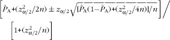
provides coverage closer to the nominal level than both the Wald and exact CIs for small sample sizes (i.e. 5–100). Third, to circumvent Wald and exact CI coverage limitations, as well as the cumbersomeness of (5), Agresti and Coull (Reference Agresti and Coull1998) suggest a modified 95% Wald interval (the ‘add 2 successes and 2 failures’ adjusted Wald interval):

where  . This interval is slightly conservative relative to the score interval but does not suffer from low coverage near 0 and 1 (for sample sizes ranging from 0 to 100) and is still closer to 95% coverage than exact intervals (Agresti and Coull, Reference Agresti and Coull1998).
3.1.1.1. Example
Assume that from a very large herd of dairy cows, n=200 animals are randomly sampled and x=26 animals test positive for MAP infection, yielding an apparent prevalence estimate of A=0.13. Using (3), a 95% CI for P A is 0.083–0.177. Exact calculations using either the binomial or F distributions yield a 95% CI from 0.087 to 0.185, while the 95% score CI is from 0.090 to 0.184. The adjusted Wald 95% CI is from 0.090 to 0.185.
If a 100(1−α)% CI is desired when there are no positive test results, an exact CI can readily be calculated using (0, 1−α1/n) (Louis, Reference Louis1981). When n≥20 and α=0.05, a good approximation to this interval is ‘the rule of three’ 95% CI=(0, 3/n) (Jovanovic and Levy, Reference Jovanovic and Levy1997). If in our last example, 0 of 200 animals test positive, then using (0, 1−α1/n), a 95% CI for P A is 0–0.0149 and using the ‘rule of three’ is 0–0.0150. Hence for this scenario, both these methods give practically the same results.
3.1.2. Bayesian approach
Here, the data are supplemented with prior information. Priors for P require distributions ranging from 0 to 1. The beta family provides a class of distributions supported on the unit interval (0–1) with a range of flexible shapes, including U-, J- and L-shaped, unimodal symmetric, right and left skewed and uniform distributions. With a binomial (n, P) likelihood, a beta(a, b) prior for P results in a beta(x+a, n+b−x) posterior for P. We can summarize posterior inference for P using either the mean or the median and 95% PI of this beta distribution.
To specify values for the hyperparameters a and b for a beta(a, b) prior, we generally use historical data and/or expert opinion. For instance, to incorporate expert opinion for apparent prevalence, we elicit what the expert believes to be the most likely value of P A in the herd. This serves as a prior point estimate, namely the prior mode of P A. Then, with a specified high probability (usually 0.95 or 0.99), the expert provides a value that P A is believed to be greater than (less than) if the prior mode is greater than (less than) 0.5. The prior mode and outer percentile (95th or 99th) are input into software programs, e.g. BetaBuster (which is downloadable from http://www.epi.ucdavis.edu/diagnostictests/betabuster.html) and the values a and b are produced as output. When little is known of the prior testing history of the herd, a diffuse prior may be used which prescribes equal likelihood to every possible value of the prevalence. A beta(1, 1) (equivalent to a uniform(0, 1)) distribution is an example of one such prior.
3.1.2.1. Example
Assume that prior to data collection we have no prior information on disease prevalence in the herd sampled in 3.1.1.1. Since the ratio of sample size to herd size (i.e. sample size (n)/herd size (N)) ⩽0.1, we assume a binomial distribution (x~bin(n, P A)) for the number of animals testing positive (Berry and Lindgren, Reference Berry and Lindgren1996). For simplicity, we also assume that Se=Sp=1 (i.e. P A=P T). The apparent prevalence can easily be estimated in WinBUGS (see Appendix B.1a). Using a beta(1, 1) prior, the posterior median and 95% PI for P A were 0.132 and 0.090–0.184, respectively. Thus, we are 95% certain that the apparent prevalence is between 0.090 and 0.184. If prior information were available on the prevalence of MAP infection in the herd, this could easily be incorporated into the Bayesian analysis. For example if prior to data collection, the herd veterinarian indicates that, based on a previous survey, he expects that 1 in 10 cows will be seropositive for MAP (mode=0.1) and he is 95% sure that P A<0.2. Inputting this information into BetaBuster, we get a beta (5.62, 42.57) prior. This beta prior has a median of 0.111 and 95% PI from 0.043 to 0.220. From WinBUGS (see Appendix B.1b) the posterior median and 95% PI for P A are 0.126 and 0.089–0.171, respectively. Note that the posterior point estimate (0.126) is intermediate between the median of the prior distribution (0.111) and the point estimate obtained from the data (0.130). In addition, we note (as is generally the case) that the posterior interval estimate (95% PI: 0.089–0.171) is narrower than the prior interval estimate (95% PI: 0.043–0.220).
3.2. Diagnostic tests
Diagnostic tests commonly used in prevalence studies of Johne's disease in live animals are based on either the identification of the etiologic agent (MAP) or detection of a serum or milk antibody response to its presence (Manning and Collins, Reference Manning and Collins2001; Collins et al., Reference Collins, Gardner, Garry, Roussel and Wells2006). Researchers typically use fecal culture as a reference MAP-detection test against which to evaluate the performance of serological tests such as the enzyme-linked immunosorbent assay (ELISA) (Manning and Collins, Reference Manning and Collins2001). However, the intermittent fecal shedding of MAP particularly during sub-clinical infection, coupled with late-stage antibody production, makes accurate and precise estimation of test characteristics challenging. Consequently, prevalence estimation methods that rely on these tests should incorporate uncertainty in values of test accuracy parameters such as Se and Sp. Priors for diagnostic tests can be derived based on the results of recent validation studies involving animals with similar characteristics to the ones about to be tested. If during a validation study for test Se, x out of n infected animals test positive for MAP, then a beta(x+1, n−x+1) is an appropriate choice of prior for Se (Vose, Reference Vose2000). This beta distribution is obtained as the posterior of Se when the validation study data are modeled as bin(n, Se) with a uniform (0, 1) prior on Se. For example, if in a recent validation study, 30 of 100 infected cows tested positive for MAP infection, then a beta(31, 71) prior for Se can be used in analysis of the future prevalence survey data. For our examples, we use two commonly-used diagnostic tests, serum (IDEXX) ELISA and fecal culture on Herrold's egg yolk (HEY) medium. Priors for these tests (see Table 1) are based on both the results of validation studies (Sockett et al., Reference Sockett, Carr and Collins1992; Collins et al., Reference Collins, Wells, Petrini, Collins, Schultz and Whitlock2005) and expert opinion.
Priors for sensitivity (Se) and specificity (Sp) of IDEXX serum ELISA and HEY fecal culture based on validation studies and updated with expert opinion

1 Most likely values of sensitivity and specificity are used as point estimates for frequentist calculations.
3.3. True prevalence
3.3.1. Frequentist approach
True prevalence (P T) of infection is the probability that a randomly-chosen unit from the source population is infected. Apparent prevalence is related to P T, Se and Sp through the equation P A=P TSe+(1−P T)(1−Sp). Among the first estimators of P T was the Rogan–Gladen-estimator (Rogan and Gladen, Reference Rogan and Gladen1978), which is obtained by substitution of estimates of P A, Se and Sp into this equation to yield

If Se and Sp are assumed known with certainty, then the standard error of T is given by: (Greiner and Gardner, Reference Greiner and Gardner2000a)

where J=Se+Sp−1 denotes the Youden index (Youden, Reference Youden1950), a combined measure of test accuracy. In practice, Se and Sp are not known with certainty (Greiner and Gardner, Reference Greiner and Gardner2000a) in which case

(Greiner and Gardner, Reference Greiner and Gardner2000a) provides a more valid quantification of uncertainty. Here,

where n 1 and n 2 are the numbers of infected and non-infected animals, respectively, in the original test validation study.
3.3.1.1. Example
Assume that a serum ELISA (Se=0.30, Sp=0.96) was used to test the herd described in section 3.1.1. Then T=0.346. If we assume that Se and Sp are known with certainty, then using (8), a 95% CI is 0.167–0.525. Using (9) with n 1 and n 2=415 and 359, respectively (Collins et al., Reference Collins, Wells, Petrini, Collins, Schultz and Whitlock2005), a more realistic 95% CI that captures the uncertainty in Se and Sp is 0.160–0.533. As is evident from this example, the discrepancy between T (0.346) and A (0.13) can be substantial. In general, the more accurate the test, i.e. the closer the Youden index is to 1, the smaller the discrepancy. Though most often P T>P A for a given herd and diagnostic test, the converse is also possible. Using a test with Se=0.30 and Sp=0.96, we note that T<A when T<0.057. Comparing the CIs obtained using formulas (3), (8) and (9), we also note that precision is greater when P A is estimated or when P T is estimated assuming that the diagnostic test's characteristics are known perfectly. In general, while differences between the precision of estimates obtained assuming known and unknown test characteristics are smaller for larger sample sizes (n 1 and n 2) of the validation studies originally used to estimate Se and Sp, the difference in bias increases since the bias in T decreases but not in A (Rogan and Gladen, Reference Rogan and Gladen1978).
The application of the Rogan–Gladen-estimator is problematic in some situations because T can be <0 or >1. In the context of MAP infection, only the former is of practical importance and can occur in a small sample with low infection prevalence when the proportion of false-positive results is greater than the apparent prevalence. The limitations of (7) are further exacerbated by the fact that when sample sizes are small and true prevalence low, the normal approximation used for calculation of CIs may not be justifiable. In particular, the condition 0<T±3s.e.(T)<1 becomes difficult to satisfy when (9) is used. For these reasons, we advise against using (7) for small samples and when prevalence is believed to be close to 0.
3.3.2. Bayesian approach
A Bayesian analysis naturally accounts for uncertainty in the values of P T, Se and Sp. Under binomial sampling, the distribution of the number of animals testing positive is given by x|(P T, Se, Sp)~bin(n, P A), where P A=P TSe+(1−P T)(1−Sp). Implicit in the use of a beta prior for the prevalence is the certainty that P T≠0. If we wish to allow for the possibility of zero infection prevalence, then we can use the mixture prior distribution: P T~beta(a, b) with probability=λ and P T=0 with probability=1−λ. The parameter λ denotes the probability that the herd is infected, and in the single herd setting is typically set equal to an expert-specified value, but can alternatively be modeled using a beta distribution (Branscum et al., Reference Branscum, Gardner and Johnson2004). A mixture prior gives a more appropriate statistical model for low prevalence or disease freedom surveys. Models that do not allow for zero prevalence will tend to produce estimates that are biased upwards. As previously mentioned, in addition to modeling P T, beta distributions are commonly used as priors for Se and Sp (see Table 1) (Hanson et al., Reference Hanson, Johnson, Gardner and Georgiadis2003b; Branscum et al., Reference Branscum, Gardner and Johnson2004). For most of the Bayesian examples in this paper, we use data collected from randomly-selected cows in 29 California dairy herds that were tested for Johne's disease using serum (IDEXX) ELISA and/or fecal culture on HEY medium.
3.3.2.1. Example
Assume that n=60 cows are randomly selected out of a herd of size 675 and suppose x=2 cows (3.3%) test positive for MAP infection using a serum ELISA. Note that here the Rogan–Gladen-estimator yields a negative prevalence estimate (T=−0.026). Since 60/675=0.089<0.10, the assumption of binomial sampling is reasonable. The probability that the herd is infected was set at λ=0.9 since 90% of herds in California were presumed infected with MAP at the time of sampling. Since no records were available from the herd regarding previous monitoring or diagnostic testing, we assume that, conditional on the herd being MAP-infected, all prevalences are a priori equally likely. This translates to P T~beta(1, 1) prior distribution. Using beta priors for ELISA Se and Sp (see Table 1), the model was fit in WinBUGS (code in Appendix B.2). The estimated (posterior median) prevalence of MAP infection in the herd was 0.02 with 95% PI from 0 to 0.453. Thus, given that 2 animals out of 60 tested positive using ELISA, we are 97.5% certain that P T<0.453. The analysis also permits inferences regarding the posterior probability that the herd was infected. Given that 2 of 60 animals tested positive, we are 57% sure that the herd was infected.
A Bayesian approach is readily implemented for all realizations of x, including x=0 and x=n. For instance, if no animals had tested positive out of 60, the posterior median and 95% PI would be P T=0 (95% PI: 0–0.237), and the posterior probability of infection would be 0.37 (see Appendix B.3).
When sample size (n)/herd size (N)>0.1, the binomial sampling approximation is no longer appropriate and the hypergeometric distribution, which is based on finite population sampling, should be used for analysis, i.e. x|(P T, Se, Sp)~hypergeometric(N, n, P A). The Bayesian Disease Freedom (BDFree) software, which can be downloaded from www.epi.ucdavis.edu/diagnostictests, contains a module for estimating P T under finite population sampling. Assume that in the previous example, all 675 cows in a known infected herd were tested and 23 were ELISA positive (i.e., the apparent prevalence is almost identical to the estimate based on the sample of 60 cows). Using BDFree (see Appendix B.4), P T=0.025 (95% PI: 0.001–0.152). The posterior probability that the herd is infected given that 23 cows test positive is 0.96.
Computational methods for prevalence estimation are much more complex for finite population sampling than for binomial sampling and we refer readers elsewhere for details (Cameron and Baldock, Reference Cameron and Baldock1998; Su et al., Reference Su, Gardner and Johnson2004).
3.4. True versus apparent prevalence
In the context of prevalence estimation, inferences for P T are preferred to inferences for P A. Nevertheless, if test Se and Sp are assumed to be constant and we want to ascertain only if P T is increasing or decreasing over time in a herd, we can make use of the linear relationship resulting from (7); P T=mP A+C where m=1/J and C=(Sp−1)/J are both constants. Consequently, if P A increases (decreases) we infer that P T increases (decreases). For these conclusions to be valid, the same diagnostic test with constant Se and Sp over time must be used on each occasion and the sampling scheme and cut-off for test interpretation must be unchanged.
4. Individual-level prevalence estimation from pooled samples
4.1. Uses of pooled testing: advantages versus disadvantages
Though pooling has been used for detection of fish pathogens in aquaculture for at least 20 years (Worlund and Taylor, Reference Worlund and Taylor1983), the use of artificially-created pools for diagnostic testing in livestock species is a recent occurrence (Nielsen et al., Reference Nielsen, Thamsborg, Houe and Bitsch2000; Borel et al., Reference Borel, Doherr, Vretou, Psarrou, Thoma and Pospischil2004; Tavornpanich et al., Reference Tavornpanich, Gardner, Anderson, Shin, Whitlock, Fyock, Adaska, Walker and Hietala2004; Letellier et al., Reference Letellier, De Meulemeester, Lomba, Mijten and Kerkhofs2005; Brinkhof et al., Reference Brinkhof, Houwers and van Maanen2006). One pooled sample can be used to determine the pathogen status of a herd (infected or non-infected), while individual-level infection prevalence can be estimated if multiple pools are tested (Cowling et al., Reference Cowling, Gardner and Johnson1999; Christensen and Gardner, Reference Christensen and Gardner2000). In this section, we focus mainly on issues related to individual-level prevalence estimation using data from pooled samples.
When sample collection costs are low relative to test cost and P<0.1 (i.e. the condition is rare) (Sacks et al., Reference Sacks, Bolin and Crowder1989; Tu et al., Reference Tu, Litvak and Pagano1994), pooled testing can be more cost- effective than individual testing and can provide more precise prevalence estimates per number of tests used (Kline et al., Reference Kline, Brothers, Brookmeyer, Zeger and Quinn1989). These advantages are based on the assumption that there is no loss of test accuracy resulting from aggregation of samples and that bias is negligible (implies moderate to small pool sizes and large sample sizes). Disadvantages of pooled testing include the need to store and handle larger volumes and the potential for loss of Se and possibly Sp compared with use of individual samples (Christensen and Gardner, Reference Christensen and Gardner2000).
4.2. Sensitivity and specificity of pooled tests
The pooled sensitivity (PSe) is the probability that a pool will test positive given that it contains at least one sample from an infected animal, while pooled specificity (PSp) is the probability that a pool will test negative given that it does not contain a sample from any infected animal (Munoz-Zanzi et al., Reference Munoz-Zanzi, Thurmond, Hietala and Johnson2006). Although several authors mention the necessity for the ‘no loss of test accuracy assumption’ (PSe=Se and PSp=Sp), especially as it applies to PSe (Kline et al., Reference Kline, Brothers, Brookmeyer, Zeger and Quinn1989; Tu et al., Reference Tu, Litvak and Pagano1995; Cowling et al., Reference Cowling, Gardner and Johnson1999; Christensen and Gardner, Reference Christensen and Gardner2000), there is a dearth of information in the animal health literature on this topic. It is assumed that PSe depends on the prevalence of the agent, its concentration in infected samples, the number of samples per pool, the mechanism by which the test identifies positivity, and the analytic and diagnostic sensitivity of the assay to be used (Munoz-Zanzi et al., Reference Munoz-Zanzi, Thurmond, Hietala and Johnson2006). For instance, an increase in pool size when testing for bovine viral diarrhea using real-time PCR (Munoz-Zanzi et al., Reference Munoz-Zanzi, Thurmond, Hietala and Johnson2006) and when testing for MAP using fecal culture (Wells et al., Reference Wells, Whitlock and Lindeman2002) has been found to decrease PSe. Others found that PSe was greater, the greater the number of infected samples per pool when testing for MAP using fecal culture (Tavornpanich et al., Reference Tavornpanich, Gardner, Anderson, Shin, Whitlock, Fyock, Adaska, Walker and Hietala2004). PSp is a function of the degree of cross contamination of the pool by other related agents. Some authors have suggested that larger pool sizes may increase PSp because of dilution of false-positive-causing analytes (Christensen and Gardner, Reference Christensen and Gardner2000). Others (Munoz-Zanzi et al., Reference Munoz-Zanzi, Thurmond, Hietala and Johnson2006) have found opposite results and have speculated that larger pool sizes increase the probability of more contaminants being included in the pool. The effect of different factors on PSp is likely to be disease- and test-dependent, and would not apply to bacterial or virus isolation, which should be perfectly specific.
Culture of fecal pools has been the testing method of choice for pooled-sample estimation of MAP infection prevalence at both the individual (Kalis et al., Reference Kalis, Hesselink, Barkema and Collins2000; Wells et al., Reference Wells, Whitlock and Lindeman2002; Tavornpanich et al., Reference Tavornpanich, Gardner, Anderson, Shin, Whitlock, Fyock, Adaska, Walker and Hietala2004) and herd level (Wells et al., Reference Wells, Godden, Lindeman and Collins2003; Kalis et al., Reference Kalis, Collins, Barkema and Hesselink2004). Compared with individual animal testing for MAP infection, pools of feces from 5–10 animals lead to substantial economic savings with commensurate minor losses in test accuracy (PSe≈Se and PSp≈Sp). In particular, PSp=Sp when testing for MAP using fecal culture.
4.3. Frequentist estimation
4.3.1. Fixed pool size and no available test information
If test Se and Sp information is not available, a simple approach uses the following formula (Kline et al., Reference Kline, Brothers, Brookmeyer, Zeger and Quinn1989; Sacks et al., Reference Sacks, Bolin and Crowder1989):

where s p=pool size, x p=number of pools testing positive and n p=total number of pools. An approximate 100(1−α)% CI for P A is:

where  p=x p/n p (empirical prevalence of positive pools).
4.3.1.1. Example
Assume that we randomly select 120 cows from a large herd. Fecal samples are obtained from all 120 and pooled into groups of 10. Fecal culture is performed on all pools and five pools test positive for MAP. Using (10) and (11) yields A=0.053 (95% CI: 0.007–0.098). Apart from the implicit assumption of perfect Se and Sp, one disadvantage of this method is that for low numbers of positive pools, negative lower confidence limits may result (Cowling et al., Reference Cowling, Gardner and Johnson1999). If in our example, x p=2, using (10) and (11), A=0.018 (95% CI: −0.007 to 0.043). When asymptotic methods fail, one can first calculate an approximate CI for p p using

and

where  p=1−p, for the lower and upper bounds, respectively (Tu et al., Reference Tu, Litvak and Pagano1994). The lower and upper 100(1−α)% confidence limits for P A are then obtained by substituting [p p]Lower and [p p]Upper for p (=x p/n p) in (10). Using (12) and (13) for x p=2, an approximate 95% CI would range from 0.003 to 0.05. Equations (12) and (13) make use of a continuity correction, bringing continuous normally-distributed variables into closer agreement with the discrete binomial distribution (Fleiss, Reference Fleiss1981). Another alternative is to calculate exact confidence intervals using (4) or from the binomial distribution using x p as the binomial variate (see Appendix A.1) and then as above, substituting [p p]Lower and [p p]Upper for p in (10).
4.3.2. Fixed pool size and imperfect test sensitivity and specificity
If information on Se and Sp is available, the conditions 1−Sp⩽p p⩽Se and Se+Sp−1>0 must hold in order to estimate P T (Tu et al., Reference Tu, Litvak and Pagano1994). We assume that PSe=Se and PSp=Sp and if Se and Sp are known, then the following formula can be used to estimate P T:

where J p=PSe+PSp−1. An approximate 100(1−α)% CI for P T is given by (Tu et al., Reference Tu, Litvak and Pagano1994):

where A p=(PSe−p)/J p.
If asymptotic assumptions fail, equations (12) and (13) may be used to obtain lower and upper confidence limits for p p, which can then be substituted into (14) for p to obtain a CI for P T (Tu et al., Reference Tu, Litvak and Pagano1994; Cowling et al., Reference Cowling, Gardner and Johnson1999). Alternatively, exact confidence limits may be calculated for p p and similarly substituted into (14) (Cowling et al., Reference Cowling, Gardner and Johnson1999). The Pooled Prevalence Calculator (PPC) (http://www.ausvet.com.au/pprev/) facilitates easy calculations of both exact and asymptotic CIs for pooled prevalence (see Appendix A.2).
If Se and Sp are not known with certainty, an approximate 100(1−α)% CI for P T is given by (Cowling et al., Reference Cowling, Gardner and Johnson1999):

where  and n 1 and n 2 (as before) refer to the number of infected and non-infected animals, respectively, used in the original test validation study. Using n 1=182 and n 2=100 (Sockett et al., Reference Sockett, Carr and Collins1992), T=0.112 (95% CI: −0.026 to 0.249). The (unrealistic) negative lower confidence limit reflects the increased difficulty in justifying large-sample normal approximations with relatively small sample sizes when test characteristic uncertainty is taken into consideration. Currently, there are no frequentist exact methods that incorporate uncertainty in Se and Sp. Thus, for reasons previously mentioned (see section 3.3.1), we advise against using (16) when prevalence is low.
4.4. Bayesian estimation
As pooled testing is most cost-effective when prevalence is low, approaches that incorporate test Se and Sp and provide realistic results (i.e. estimates and limits within the range 0–1) are particularly desirable for those situations. A Bayesian approach ensures that intervals are bounded below by 0. We assume a binomial distribution (Branscum et al., Reference Branscum, Gardner and Johnson2004) for the number of pools that test positive and thus x p|(P T, PSe, PSp)~bin(n, p p), where  . As in the case of prevalence estimation based on individual samples, beta distributions are chosen to model uncertainty in P T, PSe and PSp, and mixture models can be used to allow for zero prevalence (analogous to the development in section 3.3.2).
4.4.1. Example
Fecal samples from n=60 cows of a herd of N=2223 are obtained, randomly aggregated into 6 pools of 10 each and each pool is tested for MAP using fecal culture (Se=0.60 and Sp=0.999) (see Table 1). Two pools test positive. In a previous testing within other herds in the region, the most frequently occurring prevalence was 0.13 and the herd veterinarian is of the opinion that if MAP is present in this herd, no more than 1 in 4 animals would be infected. The herd is located in a region that has a herd prevalence of MAP infection of 95%. Using BetaBuster, we obtain a P T~beta(5.87, 33.61) given that the herd is infected. The prior probability that the herd was infected was set equal to 0.95. The results of the Bayesian analysis (see Appendix B.5 for code) were T=0.18 (95% PI: 0.08–0.32). Given that 2 of 6 pools test positive, the posterior probability that the herd is infected is 0.997.
5. Herd prevalence estimation
5.1. General concepts
5.1.1. Definition of a herd
A herd is defined as any cluster or grouping of animals (Christensen and Gardner, Reference Christensen and Gardner2000), often defined by location (Boelaert et al., Reference Boelaert, Walravens, Biront, Vermeersch, Berkvens and Godfroid2000; Tavornpanich et al., Reference Tavornpanich, Gardner, Anderson, Shin, Whitlock, Fyock, Adaska, Walker and Hietala2004) but may also be defined by size (Baggesen et al., Reference Baggesen, Wegener, Bager, Stege and Christensen1996), intended purpose (Christensen et al., Reference Christensen, Baggesen, Nielsen and Stryhn2002), clinical signs (Wells et al., Reference Wells, Godden, Lindeman and Collins2003), age (Boelaert et al., Reference Boelaert, Walravens, Biront, Vermeersch, Berkvens and Godfroid2000) or combinations of the above. The herd (or herd-level) prevalence (HP) of infection in a population of herds is defined as the proportion of infected herds in the population:

In contrast to individual-level prevalence surveys, the unit of analysis in herd-level surveys is the herd or whole group.
5.1.2. Herd testing
Herd testing is typically undertaken to classify the status of a herd (or herds) with respect to disease or infection. If the goal is to make statistical inferences regarding HP, then herds to be tested should be selected using a random sampling scheme that is likely to ensure disperse coverage of the targeted region. Typically, a two-stage sampling design is used where M herds are randomly sampled in the first stage and then n i animals are sampled from each herd i, i=1, …, M. Selection of animals within herds may be done randomly or not depending on the survey goals (e.g. estimation of within-herd prevalence versus classification of herds by infection status). In the veterinary literature, herd tests and herd-prevalence estimation have been conducted for health certification (Cameron and Baldock, Reference Cameron and Baldock1998; Kalis et al., Reference Kalis, Collins, Barkema and Hesselink2004) and diagnostic test evaluation (Sergeant et al., Reference Sergeant, Whittington and More2002; Wells et al., Reference Wells, Godden, Lindeman and Collins2003; Tavornpanich et al., Reference Tavornpanich, Gardner, Anderson, Shin, Whitlock, Fyock, Adaska, Walker and Hietala2004), to identify herd-level risk factors for individual and herd-level infection (Delafosse et al., Reference Delafosse, Castro-Hermida, Baudry, Ares-Mazas and Chartier2006), and for assessments of exposure to etiologic agents (Turnquist et al., Reference Turnquist, Snider, Kreeger, Miller, Hagstad and Olcott1991).
Unlike individual-level testing, herd-level testing is a function of two cut-off points: the positivity threshold of the diagnostic test(s) used to classify individual animals as infected or not and the herd cut-off value for classifying herds as infected or not (Christensen and Gardner, Reference Christensen and Gardner2000). The herd cut-off value may be an absolute number (e.g. ≥2 infected animals classifies the herd as infected) or a percent (e.g. ≥1% of animals infected classifies the herd as infected).
5.1.3. Herd sensitivity and specificity
Herd-level sensitivity (HSe) is the proportion of infected herds in which the number of animals with positive test results equals or exceeds the herd-level cut-off (Martin et al., Reference Martin, Shoukri and Thorburn1992). With the decision rule that uses a cut-off of ≥1 positive test result to classify the herd as positive, HSe=1−(1−P A)n (Christensen and Gardner, Reference Christensen and Gardner2000), where n denotes the number of animals tested from the herd. HSe increases with increased n, P A (and hence P T), and Se and decreases with increased within-herd cut-off for a positive test result (Martin et al., Reference Martin, Shoukri and Thorburn1992; Donald et al., Reference Donald, Gardner and Wiggins1994).
Herd-level specificity (HSp) is the proportion of non-infected herds that test negative in the population of herds, i.e. the proportion of non-infected herds in which the number of animals with positive test results is less than the within-herd cut-off (Martin et al., Reference Martin, Shoukri and Thorburn1992). With a cut-off of 1 for herd infection, HSp=Sp n (Christensen and Gardner, Reference Christensen and Gardner2000). HSp increases with increased cut-off values and Sp, and decreases as n increases (Martin et al., Reference Martin, Shoukri and Thorburn1992; Donald et al., Reference Donald, Gardner and Wiggins1994).
Herd-level test characteristics are also affected by within-herd correlation in disease or infection states (Donald et al., Reference Donald, Gardner and Wiggins1994). For a detailed account of the effect of correlation on herd-level test characteristics, the reader is referred to Donald et al. (Reference Donald, Gardner and Wiggins1994) .
5.2. Frequentist approach
Analogous to individual-level prevalence, true herd-level prevalence is estimated by (Wagner and Salman, Reference Wagner and Salman2004):

where  is the estimated apparent herd prevalence (i.e. number of test-positive herds/total number of herds tested) and J H=HSe+HSp−1. An approximate 100(1−α)% CI for HP T is given by

where n H is the number of herds tested. The application of (17) and (18) to herd prevalence estimation is problematic as it is necessary to assume common values for HSe and HSp. This also implies a common value for P A, which would unrealistically imply constant infection prevalence from herd to herd. As a result, we discourage routine use of these formulas in favor of the Bayesian approach to herd prevalence estimation presented in the next section.
5.3. Bayesian approach
In the Bayesian setting with binomial sampling, we model within-herd prevalences as independent and identically distributed according to a common prevalence distribution, and we assume that the test's Se and Sp are invariant from herd to herd. The number of animals that test positive in each herd is modeled as x i~bin(n i, P TiSe+(1−P Ti)(1−Sp)) with independent beta priors for Se and Sp. As in the single herd setting, each within-herd prevalence is modeled according to a mixture distribution that models zero infection prevalence with probability 1−HP T where HP T denotes the herd-level prevalence in the region. For infected herds, the within-herd prevalence distribution is given by P Ti~beta(μψ, ψ(1−μ)) where μ is the mean true prevalence in the population and ψ is a parameter related to the variance of the prevalence distribution that flexibly allows for disperse (e.g. uniformly distributed) or very similar infection prevalences among herds (Branscum et al., Reference Branscum, Gardner and Johnson2004). Large values of ψ indicate less variability so that within-herd prevalences concentrate around μ, while small values of ψ correspond to more heterogeneity of prevalence values across herds (Donald et al., Reference Donald, Gardner and Wiggins1994; Branscum et al., Reference Branscum, Gardner and Johnson2004).
The mean prevalence (μ) and ψ are typically modeled with beta and gamma distributions, respectively (Hanson et al., Reference Hanson, Johnson and Gardner2003a; Branscum et al., Reference Branscum, Gardner and Johnson2004), but other distributions can be used. A Bayesian approach allows not only for herd-level prevalence estimation but also provides a straightforward means to make predictive inferences about herds not tested during the survey. It is also possible to estimate the intracluster correlation coefficient for true prevalence among the study herds (Branscum et al., Reference Branscum, Gardner, Wagner, McInturff and Salman2005b).
5.3.1. Example
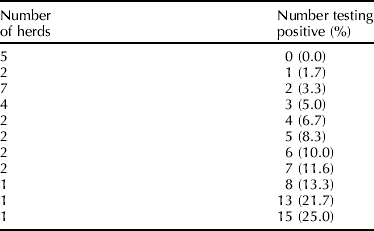
Using a two-stage sampling scheme, 29 dairy herds were randomly selected from dairy practices in central California. Random samples of 60 cows were selected from each herd and tested for MAP infection using serum ELISA. Data from the 29 herds are summarized in Table 2 and we assume a binomial distribution for the numbers of animals testing positive. Based on expert opinion, 60% of herds in this region of California were expected to be infected at the time of sampling with a one-sided 95% limit of 30% (i.e. the expert was 95% sure that the proportion of MAP-infected herds was greater than 0.30). BetaBuster yields a beta(4.8, 3.6) prior for HP T. The ELISA test Se and Sp are modeled as in previous sections (see Table 1). The mean prevalence (μ) and ψ were modeled using beta(3.283, 17.744) and gamma (4.524, 0.387) priors, respectively (see Hanson et al., Reference Hanson, Johnson and Gardner2003a, for rationale and method of derivation). Finally, a mixture model was used because some herds in the region might be free of MAP-infected animals. The model was fit using WinBUGS (see Appendix B.6 for code).
Results of herd prevalence survey of MAP infection using IDEXX ELISA in 29 central California dairies (60 cows tested per herd)
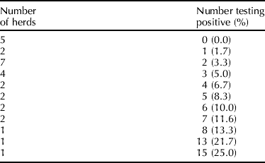
The estimated posterior median of HP T was 0.51 with 95% PI from 0.27 to 0.80, while the mean prevalence among infected herds was μ=0.18 (95% PI: 0.08–0.33). The estimated posterior prevalence distribution characterizes the within-herd prevalences in the region. At the time of sampling, 49% of the herds in the region were estimated to be free of MAP infection, 59% of the herds in the region had infection prevalence <0.05 and 82% had infection prevalence <0.2.
6. Comparison of prevalence
6.1. Sequential testing in herds
Investigators often sequentially test herds as a means of evaluating the effectiveness of management practices or interventions aimed at controlling or eradicating MAP infection, or to longitudinally monitor changes in infection prevalence. On other occasions, prevalence might be compared between two herds or two groups of animals within herds to determine whether or not they differ. Depending on the goal of the survey, the samples may or may not be regarded as statistically independent.
6.2. Frequentist comparison of population prevalence
6.2.1. Independent samples
To determine if two apparent prevalences  are statistically different based on test results obtained from random samples of animals from distinct herds, a chi-square (χ2) test of homogeneity of proportions may be performed (Agresti, Reference Agresti1996);

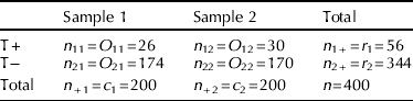
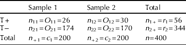
where both i and j=1, 2, O ij and Ê ij are the observed and (estimated) expected values, respectively, in the ith row and jth column of a 2×2 contingency table (see Table 3) and  . The estimated expected value is Ê ij=r ic j/n, where r i and c j are the ith row and jth column totals, respectively. The statistical hypothesis to be tested is:
 versus
 with degrees of freedom (df)=(R−1)(C−1)=1, where R and C are the number of rows and columns, respectively (R=C=2 for 2×2 tables). The null hypothesis (H 0) is rejected if χ2>χ2df=1,1−α where χ2df=1,1−α is the value corresponding to the 1−α percentile of the χ12 distribution and α=type I error probability.
2×2 Contingency table for prevalence data
6.2.1.1. Example
Assume that 1 year after an initial testing, the herd described in section 3.1.1 is again tested for MAP, and 30/200 cows have positive test results, yielding an apparent prevalence  (Table 3). To test whether
 are statistically different, we use (19) and α=0.05. This yields χ2=0.33<χ21,0.95=3.84, hence we do not reject H 0 (i.e., there is no statistical evidence suggesting a change in apparent prevalence). A 100(1−α)% CI for
 is

Hence,  with 95% CI of −0.05 to 0.09. For statistically independent samples, if any Ê ij<5, the Fisher exact test is recommended to compare independent proportions (Rosner, Reference Rosner2000).
6.2.2. Dependent samples
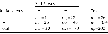
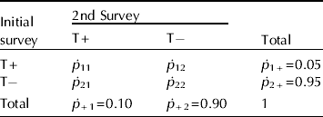
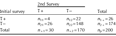
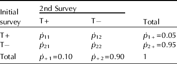
In the previous example, if on both occasions the same cows were sampled (matched pair or repeated measures design), the data may be presented as in Table 4 and a McNemar's χ2 test of homogeneity of proportions that accounts for correlated data should be performed. Here, (Agresti, Reference Agresti1996)

where n 12 and n 21 are the numbers of cows with discordant test results (T+T− and T−T+, respectively) at the initial and subsequent sampling. If n 12≠n 21 then  and (21) can be used to test
 versus
 . Again H 0 is rejected if χ2>χ2df=1,1−α. Using α=0.05, χ2=0.333<3.84, hence we do not reject H 0.
2×2 Contingency table for prevalence data (matched pairs)
n p=the total number of pairs.
For paired binary data, a 100(1−α)% CI for  is (Agresti, Reference Agresti1996)

where p ij=n ij/n p, p 1+=p11+p12, p +1=p11+p21 and n p refers to the number of cows (each tested twice). Hence, if the same cows were tested on both occasions, the estimated difference between the apparent prevalences is 0.02, with 95% CI of −0.05 to 0.09. Both this CI and the one calculated in the previous section indicate that the data are consistent with  being as large as 9% more and as small as 5% less than
 . If n 12+n 21<20, an exact version of McNemar's test is recommended (Rosner, Reference Rosner2000) (see Appendix A.3).
With data subject to misclassification (i.e. Se and Sp both <1), there is no straightforward frequentist method for testing differences between true prevalences. However an informal test of the difference between two true prevalences may be performed by checking for overlap of their individual CIs with adjustments made for multiple comparisons since a collection of separate 100(1−α)% CIs may have joint confidence less than 100(1−α)%. Overall, caution should be exercised when applying this conservative procedure to Wald CIs. Compared with standard hypothesis testing, the method both rejects the null hypothesis less often when it is true, and fails to reject the null more frequently when it is false (Schenker and Gentleman, Reference Schenker and Gentleman2001).
6.3. Bayesian comparison of population prevalence
Using a Bayesian approach, inferences can be made for differences in true prevalences between two (or more) true population prevalences. Assuming independent binomial sampling and that both herds (section 6.2.1) were tested for MAP infection using the same serum ELISA (Table 1), a Bayesian model for the data is  where

 for j=1, 2 and beta priors are used for
 , Se and Sp. We require informative priors for Se and Sp to mitigate lack of identifiability (i.e. ensure that prevalences are estimable). Here, based only on the data, x j/n j estimates
 and we require additional input about test accuracy to estimate true prevalence. With the data and expert-elicited information about Se and Sp, inferences for
 can be made.
6.3.1. Example
Assume that based on the presence of culture-confirmed clinical cases of Johne's disease, both herds are known to be infected with MAP. Suppose, however, that no records of previous test results are available and, hence, the magnitude of within-herd prevalence of MAP infection is unknown. We thus use uniform priors for  and

 . The ELISA Se and Sp are modeled as in previous sections (Table 1), and the model is fit in WinBUGS (see Appendix B.7 for code). The posterior median of
 is 0.08 with 95% PI from −0.24 to 0.44. On the basis of the posterior probability,

 , we are 71% certain that herd 2 has a higher true prevalence than herd 1.
A Bayesian approach also facilitates comparisons of prevalence when different diagnostic tests are used in the two herds. For example, if herd 2 was tested with fecal culture and Se and Sp are modeled as in previous sections (see Appendix B.8 for code), the posterior median of  is −0.09 with 95% PI from −0.62 to 0.29. Given that the posterior probability
 , we are 31% certain that herd 2 has a higher true prevalence than herd 1
 and
 .
6.4. Reporting of results
For presentation of results based on frequentist or Bayesian analysis of prevalence data based on hypothesis tests, we encourage the use of interval estimates (e.g. 95% CIs or PIs) rather than, or in conjunction with, P-values or posterior probabilities. Whereas CIs and PIs help to reveal whether different statistically significant (or insignificant) results have different implications for policy or intervention decisions, P-values, which reduce results into a significant–non-significant dichotomy, obscure quantitative differences between results.
7. Sample size and power
7.1. Relevance of sample size estimation
A critical aspect of the planning phase of a prevalence survey is the estimation of the number of individuals or groups of individuals needed. The sample size determines the precision of our final estimates and ultimately influences whether the survey will be able to address the research questions of interest. Limited time and resources dictate that prior to performing a study, an investigator should be reasonably assured that enough individuals are available so that estimates can be generated with the requisite precision. Consequently, sample size calculations are standard requirements for research grant proposals. Because the components of these calculations must be hypothesized, only estimates can be obtained for any proposed study. This uncertainty becomes more pronounced in prevalence surveys when accuracy of case identification and precision of estimates is also dependent on diagnostic test characteristics. Bayesian approaches to sample size calculations for prevalence surveys account for uncertainty in parameter values (e.g. for Se and Sp) and for data subject to misclassification. As a result, they are computationally intensive and cannot be directly implemented in WinBUGS (see, for example, Johnson et al., Reference Branscum, Gardner and Johnson2004; Branscum et al., Reference Branscum, Gardner and Johnson2006). For this reason, we present only methods for frequentist sample size calculations in this section and point the interested reader to other sources covering the general methodology for Bayesian sample size determination (Adcock, Reference Adcock1997; Rahme et al., Reference Rahme, Joseph and Gyorkos2000).
7.2. Sample size required to estimate true and apparent prevalence with a given precision
Precision of an estimate may be defined as the width of its (100−α)% CI. The sample size necessary for estimating P A and P T, respectively, within a given error margin (Δ) is given by (Greiner and Gardner, Reference Greiner and Gardner2000b):

and (Greiner and Gardner, Reference Greiner and Gardner2000a)

respectively, where  is an a priori estimate of P A (for example, obtained via pilot surveys or expert opinion) and Δ=half the CI width, which may be either an absolute number or a percentage of
 (or
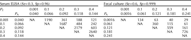
 ). Table 5 provides estimates of the number of cows necessary for testing to estimate P T for MAP infection when Δ ranges from 0.10 to 0.20, given a priori estimates of P A for testing with serum ELISA (Se=0.30, Sp=0.96) and fecal culture (Se=0.60, Sp=0.999) and assuming that the test characteristics are known. For fixed
 (
 ), as Δ increases (decreases), the required sample size decreases (increases), while for fixed Δ, as Se and/or Sp increase (decrease), the required sample size decreases (increases). Thus, the sample size required to estimate P T (P A) will be inversely proportional to the desired precision. If Se and Sp are not assumed to be known, then (24) can be generalized to adjust for uncertainty in Se and Sp using (Greiner and Gardner, Reference Greiner and Gardner2000a)

where B=Se(1−Se)/n 1, C=Sp(1−Sp)/n 2, and n 1 and n 2 are as previously defined for (9).
Sample sizes to estimate hypothesized true prevalences ( T) with a given precision (Δ) based on a priori apparent prevalence estimates (A) for serum ELISA and fecal culture assuming known sensitivity (Se) and specificity (Sp)

NA=not applicable.
7.3. Sample size to detect a difference in prevalence
Sample size calculations to detect prevalence differences have four fundamental components: the significance level or the probability of falsely concluding that there is a difference when none exists (α=probability of type I error), the probability of falsely concluding that there is no difference when there is one (β=probability of type II error), the variance of the parameter to be estimated and, most critically, the size of the parameter itself, i.e. the difference to be detected (Wittes, Reference Wittes2002).
7.3.1. Independent random samples
To calculate the sample size (n s=n 1+n 2) necessary to detect a difference  from two independent random samples, we use (Rosner, Reference Rosner2000):

and n 2 is computed based on k=n 2/n 1 where k is usually determined by the investigator. Here,  ,
 . A two-tailed hypothesis test is implied by (26), i.e.,
 versus
 . Common choices of α and 1−β are 0.05 and 0.8, respectively, and total sample size (n s) is minimized for k=1 (n 1=n 2). To estimate sample sizes based on one-tailed hypotheses (to identify either an increase or decrease in P A), z α/2 is substituted with z α in (26). However, if the inherently two-tailed χ2 statistic is to be used to test differences in prevalences, then the sample size estimation must be two-tailed to avoid sample size underestimation. One-tailed sample size calculations should be performed only if a one-tailed test is to be used to determine a difference in prevalence during data analysis (Lachin, Reference Lachin1981).
7.3.1.1. Example
Assume that two large herds have prevalences of MAP infection of  . We wish to determine if
 . We therefore calculate the required number of animals to sample in order to have a probability of 0.8 of detecting
 if such a difference exists. Using α=0.05 and 1−β=0.8 and assuming that equal numbers of animals (k=1, i.e. n 2=n 1) are available to randomly sample, (26) yields n 1=685 and sample size (n s)=1370.
Sometimes sample sizes need to be calculated to detect a change in test prevalence of MAP infection between two time points in a single herd. Sampling at the first time point may already have occurred when the need for the sample size calculation arises and economic considerations may influence whether the same number of cows can be tested at the second sampling.
7.3.1.2. Example
Assume that we have a very large herd. In an earlier random sample of 600 cows, 60 tested positive, i.e.,  . New management practices were introduced to reduce the prevalence of MAP infection and, 1 year later, we wanted to evaluate if the apparent prevalence has decreased by 5%
 . Costs of testing have increased and total costs would be reduced if testing less than 600 animals were possible. First, we need to calculate the ratio of numbers of animals necessary to sample in order to have a probability of 0.8 of detecting this difference (0.05) in prevalence if it exists. Using α=0.05 and 1−β=0.8 and assuming that equal numbers of animals are available to sample (randomly), the implied one-sided hypotheses are
 (Roussas Reference Roussas2003). We assume for simplicity that the data are statistically independent because of the time between the two sampling dates.
We first calculate the total sample size as if equal sized samples (i.e. n 2=n 1) were to be used, denoted n s(k=1), using z α=0.05 (one-sided hypothesis) in (26). This yields ns(k=1)=684. We then make use of the following relationships (Altman, Reference Altman1991):


From (27) and (28), n 1=n s(k=1)(1+k)/4k. Since 600 animals have already been sampled, we let n 1=600 and ns(k=1)=684 (from above). This yields k≈0.398 and n 2=239. Hence, we sample 239 cows at the second sampling and 839 cows in total.
7.3.2. Dependent samples
The number of paired observations (n p) necessary to detect a difference in P A estimated from testing each cow at two different time points is given by (Lachin, Reference Lachin1992):

where  12 and 21 are the a priori probabilities that a cow will have test results T+T− and T−T+, respectively, at the two testing times (see Table 1, Appendix A.4). In the context of a group of animals tested at two time points, n p refers to the number of pairs of tests to be done (i.e. the number of animals to be tested).
7.3.2.1. Example
Assume that we have a large herd known to be infected with MAP. We wish to determine if the prevalence of infection is increasing in the herd and thus plan to select a group of cows and test them longitudinally at two time points. We assume based on previous experience with other herds and with the diagnostic test to be used that ~87% of cows tested will have the same test result at both testings. In addition, we assume that  and
 , respectively (see Appendix A.4). Hence 12+21=0.13 and 21−12=0.05. Using α=0.05, z α (one-sided hypothesis) and 1−β=0.8, from (30), n p≈318 pairs of tests (318 cows).
7.4. Sample size based on true prevalence
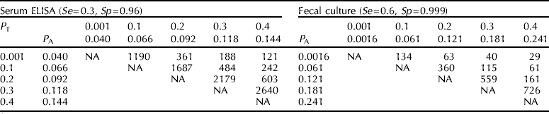
Sample sizes to detect differences in P T are done by first determining the difference in P T that is important to identify. The Rogan–Gladen estimator (7) is used to calculate the equivalent difference on the P A scale and then equation (26) or (30) is used to find the sample size necessary to detect the difference on the P A scale. We recommend that sample size estimation be done based on true rather than apparent prevalence estimates (see Table 6), wherever possible.
Sample sizes (numbers in each group)Footnote 1 required to detect differences in true prevalence (P T) for independent samples (α=0.05, 1−β=0.80 and k=1(n 2=n 1))
1 Table is symmetrical around the diagonal descending from left to right.
NA=not applicable.
7.5. Sample size required to estimate individual-level prevalence from pooled samples
Formulas for numbers of pools required to estimate individual level true and apparent prevalence can easily be derived given corresponding variance formulas (Tu et al., Reference Tu, Litvak and Pagano1994; Cowling et al., Reference Cowling, Gardner and Johnson1999). For fixed pool sizes, the formula for number of pools necessary to estimate P A within a given error margin (Δ) is

If an a priori estimate is given of the prevalence of positive pools (p), then:

Given an a priori estimate of true prevalence, when Se and Sp are assumed known

If Se and Sp are not known,

where  , B p=PSe(1−PSe)/n 1, C p=PSp(1-PSp)/n 2 and n 1 and n 2 (as before) refer to the number of infected and non-infected animals, respectively, used in the original test validation study. As in the case of individual samples, Δ may either be a constant or a percentage of the prevalence to be estimated. Comparing pool sizes of 5 and 10, we note that for a given a priori P A (or P T), PSe, PSp and Δ, pool sizes of 10 require overall fewer individual samples (see Table 7).
Sample sizesFootnote 1 required to estimate hypothesized true prevalences (T) with a given precision (Δ) based on an a priori apparent prevalence estimate (A) using pooled fecal culture with known sensitivity (PSe=0.6) and specificity (PSp=0.999)

1 Numbers of pools in parentheses.
NA=not applicable.
7.6. Sample size required to estimate herd prevalence
Sample size calculations for estimation of herd prevalence have both within-herd and among-herd components. Determination of the sample size to detect infection is an important first step in correctly determining the MAP infection status of each herd. In the context of a herd prevalence survey of M herds (h 1, h 2, …, h M) the number of samples required to detect at least one truly infected animal in the ith herd (h i) (where i⩽M), assuming binomial sampling, is given by (Christensen and Gardner, Reference Christensen and Gardner2000):

where C is the level of confidence (e.g. 95%) in detecting at least 1 truly infected animal (i.e. HSe) given an a priori specified true prevalence for that herd  and Se i and Sp i are the test's sensitivity and specificity in that herd respectively. Because herd-specific values of Se i and Sp i are not usually known, sensitivities and specificities are usually assumed to be invariant across herds. Thus the required sample size for each herd is a function of true prevalence, the desired confidence and the diagnostic test's Se and Sp. The total number of animals necessary to sample in order to have a confidence C to detect at least 1 infected animal in each herd is given by:

Corrections to (35) and (36) can be made for finite population sampling (see, for example, Martin et al., Reference Martin, Shoukri and Thorburn1992).
If within-herd prevalence estimates are not required, after initial sample size calculation using (36) above, risk-based (targeted) sampling may be used to select animals with a greater likelihood of being infected for testing if prior knowledge of risk factors for infection (e.g. previous diagnostic test results, clinical signs, etc.) is available (Christensen and Gardner, Reference Christensen and Gardner2000). For a given sample size, risk-based sampling increases the confidence to detect at least one infected animal in a herd when compared with random sampling. This has been substantiated by results from a number of studies (Nielsen et al., Reference Nielsen, Enevoldsen and Grohn2002a; Tavornpanich et al., Reference Tavornpanich, Gardner, Carpenter, Johnson and Anderson2006). Conversely, risk-based sampling can be used to reduce the sample size necessary to achieve a herd diagnosis for fixed confidence level.
The number of herds required to estimate true herd prevalence (HP T), within a given error margin (Δ) is given by (Humphry et al., Reference Humphry, Cameron and Gunn2004):

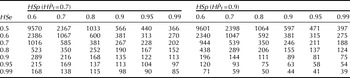
where n H=the estimated number of herds, Ω=Hse(H  ), Π=(1−HSp)(1−H ), Δ=prescribed error margin, J H=HSe+HSp−1 and z α/2 as before, refers to the 1−α/2 percentile of the standard normal distribution. The test's HSe and HSp are both pre-specified by the investigator and therefore assumed known without error. Table 8 provides estimates of the number of herds required to estimate HP T=0.7 and 0.9, respectively, within an error margin (Δ)=0.1 with 95% confidence.
Number of herds required to estimate hypothesized true herd prevalences of 0.7 (H T=0.7) and 0.9 (H T=0.9) with precision (Δ=0.1) and 95% confidence (z α/2=1.96) for different combinations of herd sensitivity (HSe) and herd specificity (HSp)

7.7. Sample size required to substantiate freedom from infection
Strictly speaking, to unequivocally demonstrate freedom from MAP infection in a herd or in a group of herds from a well-defined geographical region, all animals should be tested using a perfect test. However, a sample may be used to establish with prescribed probability that infection, if present, is below a predetermined level, i.e. a certain minimum expected prevalence (also known as design prevalence). For a herd, the minimum expected prevalence of infection would be the minimum prevalence expected if infection were actually present (Cameron and Baldock, Reference Cameron and Baldock1998). This prevalence estimate should be based on knowledge of the disease and its risk factors, knowledge of the herd itself (including previous results of surveillance and disease-related interventions) and knowledge of the Se and Sp of the diagnostic test to be used. At the regional level, the minimum accepted herd prevalence would be the lowest (non-zero) unacceptable herd prevalence, based on economic or political factors (Cameron and Baldock, Reference Cameron and Baldock1998). For substantiation of freedom from infection, two-stage sampling is usually employed. Sample sizes for both herd-level and within-herd testing to establish that infection is below a specified prevalence in a given region may be estimated using the ‘Freedom from Disease’ drop-down menu within the ‘Survey Toolbox’ or ‘FreeCalc’, which are both available at www.vetschools.co.uk/EpiVetNet/Sampling_software.htm (see Appendix A.5).
7.7.1. Example
Assume that in a region with 1000 dairy herds (herd sizes of 500–1500 cows) where the herd prevalence of MAP infection was initially 90%, substantial eradication efforts are undertaken and it is now claimed that the herd prevalence is below 50%. Veterinary authorities expect that, within any given herd, 2% or more of the animals will be infected if MAP is present. Fecal culture (Se=0.60, Sp=0.999) is to be used for testing. Using the modified hypergeometric exact formula within the Survey Tool Box with HSe=0.95 and HSp=0.98, and 95% confidence and power, we calculate that if 8 herds are chosen randomly and ⩽1 herd tests positive, we can be ~95% confident that HP T<0.5 (see i–iv, appendix A.5). The Survey Tool Box also calculates the numbers of animals necessary to sample (based on herd sizes) in order to be ~95% certain that infection, if present, is ⩽2%, given type I (1-HSe) and type II (1-HSp) errors of 0.05 and 0.02, respectively (see v–viii, appendix A.5). The survey would then be conducted by randomly sampling 8 herds and then choosing random samples of between 402 and 455 cows from herds of between 500 and 1500 respectively. If >2 animals test positive for MAP in at least 2 of the 8 herds, then the survey has not provided evidence that HP T<0.5. However, if either 0 or 1 herd has >2 animals testing positive, then we can conclude with more than 95% confidence that the true herd prevalence (HP T) of MAP infection in the region is <0.5 and where present, the true individual-level prevalence (P T) of MAP infection is <0.02.
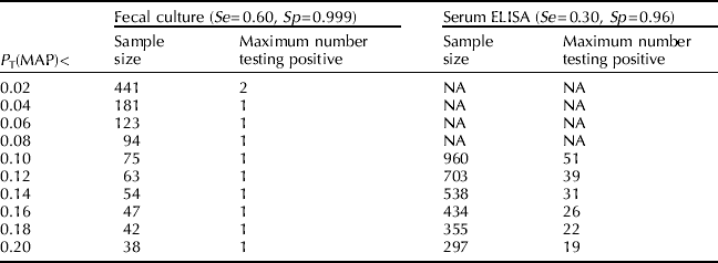
For a given herd, the lower the minimum expected prevalence and the more inaccurate the diagnostic test, the greater the sample size necessary to substantiate freedom from infection (Cameron and Baldock, Reference Cameron and Baldock1998). Given a herd of 1000 cows and that diagnostic testing is to be done using fecal culture (Se=0.60 and Sp=0.999) or ELISA (Se=0.30 and Sp=0.96), Table 9 provides sample size estimates and maximal numbers of animals testing positive in order to establish with 95% confidence (HSe) and 98% power (HSp) that MAP infection, if present, is below a given true prevalence.
Number of cows necessary to sample in a herd of size 1000 to establish with 95% confidence (HSe) and 98% power (HSp) that Mycobacterium avium subspecies paratuberculosis (MAP) infection, if present, is less than a given true prevalence (P T)

NA=not applicable (herd size too small).
Bayesian approaches to sample size determination for single herd and regional disease freedom surveys have also been developed (see, for example, Johnson et al., Reference Branscum, Gardner and Johnson2004; Branscum et al., Reference Branscum, Johnson and Gardner2006). However, computationally-complex simulation-based approaches are needed for their implementation and thus we do not present them here.
7.8. Power calculations
7.8.1. Relevance of power calculations
In the context of detecting differences in prevalences, power (1−β) is the probability that the results of the study will be statistically significant given a specified difference between groups (Goodman and Berlin, Reference Goodman and Berlin1994). Consequently, power is of direct relevance in the design phase of a study, as a means of determining the likelihood of ultimately detecting a true difference between prevalences given constraints on sample size (due to cost, availability of subjects or other factors). Post-hoc power calculations, though often performed by researchers, are of limited value in both study interpretation and evidence-based decision-making. Instead, CIs should be used to evaluate the extent to which the differences (in prevalence) are or are not compatible with the data (Goodman and Berlin, Reference Goodman and Berlin1994).
7.8.2. Power estimation (statistically independent samples)
From (26), the power to detect a difference  using a two-sided test is given by (Rosner, Reference Rosner2000):

where  are as defined in section 7.3.1 and Φ(x) denotes the standard normal cumulative distribution function evaluated at x.
7.8.2.1. Example
Assume, as in the second example of section 7.3.1, that having previously sampled 600 cows  , we wish to detect a possible decrease in prevalence of MAP infection of 5% at a subsequent sampling i.e.,
 . However, funding dictates that only 160 cows can be tested. Thus, we estimate the probability of detecting this difference in prevalence, if it exists. Using α=0.05 and k=0.267, power=Φ(0.395)=0.65. If 160 cows are sampled, there is a probability of 0.65 of detecting a change of 0.05 in apparent prevalence. If we were to sample 240 animals (k=0.398), power=0.80.
7.8.3. Power calculations (statistically dependent samples)
From (30), with matched pairs or repeated measures data, the power to detect a difference  is given by:

where n p, p 12, p 21 and z α/2 are as defined in section 7.3.2.
7.8.3.1. Example
Assume that for the herd described in section 7.3.2, testing costs dictate that only 540 tests can be performed (270 animals). Using the information in section 7.3.2 with n p≈270, from (39) Φ(Z β)=0.64 and power=0.74. Hence, there is a 74% chance of detecting an increase in apparent prevalence of 0.05, if it occurred.
8. Conclusion
Frequentist approaches to true prevalence estimation are easy to use but suffer from serious statistical limitations when prevalence is low, sample sizes are small and uncertainty in Se and Sp is to be incorporated into the precision of estimates. These limitations are easily overcome in a Bayesian context and we recommend that investigators use Bayesian methods for prevalence estimation, wherever appropriate.
Acknowledgments
The study was funded through the Johne's Disease Integrated Project and was supported by USDA–CSREES–NRI grant number 2004-35605-14243 and the Center for Food Animal Health, University of California, Davis, CA.
Appendix A
1. For
 A=x/n (x=1,2, …, n−1), an exact 100(1−α)% CI may be calculated by solving the following equations:(1)and(2)to obtain upper and lower confidence bounds, respectively. For x=0 the lower bound is 0 and, for x=n, the upper bound is 1. An Excel spreadsheet for calculation of exact 100(1−α)% CIs is available from the authors on request.
2. The pooled prevalence calculator (PPC) can be used to calculate prevalence estimates and CIs (asymptotic and exact) for the following scenarios:
• Individual-level prevalence using a fixed pool size and assuming a perfect test.
• Individual-level prevalence using a fixed pool size and known sensitivity (Se) and specificity (Sp).
• Individual-level prevalence using a fixed pool size and uncertain sensitivity (Se) and specificity (Sp)Footnote 1.
The following inputs are required:
• Pool size (S p)
• Number of pools (n p)
• Number of pools testing positive (x p)
• Test sensitivity (Se)Footnote *
• Test specificity (Sp)Footnote *
• Sample size used (in original study) to estimate sensitivity (n 1)Footnote **
• Sample size used (in original study) to estimate specificity (n 2)Footnote **
• Lower and upper confidence limits
The output provides:
• Individual-level prevalence estimate
• Confidence limits (exact or asymptotic as specified by user)
3. McNemar's exact test
4.
Table 1.2×2 Contingency table for prevalence data (matched pairs)
Given
11+22=0.87, 11+12=0.05, 11+21=0.10, 21+22=0.95, 12+22=0.90, then 21−12=0.05 and 21+12=0.13, where ij=ij/n p.5. Sample sizes necessary to substantiate freedom from disease (i.e. prevalence below a prescribed value) may be calculated using the ‘Freedom from Disease’ drop-down menu within the ‘Survey Toolbox’ or ‘FreeCalc’. Both are available at www.vetschools.co.uk/EpiVetNet/Sampling_software.htm. The following steps are necessary:
(i) Define the minimum expected prevalence at the herd level.
(ii) Define the acceptable level for a Type I error (concluding that the herd-level prevalence is not above the minimum expected herd-level prevalence when it is so).
(iii) Define the acceptable level for a Type II error (concluding that the herd-level prevalence is above the minimum expected herd-level prevalence when it is not).
(iv) Calculate the no. of herds to be sampled using FreeCalc (Cameron and Baldock, Reference Cameron and Baldock1998). To do the calculation, one has to first choose an HSe and HSp which will allow you to determine the number of herds necessary to substantiate freedom from disease. This is done by trial and error. (The program also calculates the maximum number of positive herds to be expected if the population is to be considered disease free.)
(v) Define the minimum expected (design) prevalence within herds.
(vi) Define the Type I error=1−HSe (concluding that the individual-level prevalence is not above the minimum expected within-herd prevalence when it is).
(vii) Define the Type II error rate=1−HSp (concluding that the individual-level prevalence is above the minimum expected within-herd prevalence when it is not).
(viii) Calculate the no. of animals to be sampled from each herd inputting, each time, the respective herd's size. The program provides the maximum allowable number of positive animals if prevalence below the given level is to be substantiated.

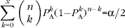


 ij/n p.
Appendix B. WinBUGS code
1. Apparent prevalence

2. Low prevalence (Rogan–Gladen-estimator <0)

3. Apparent prevalence=0

4. Hypergeometric sampling using Bayesian Disease Freedom (BDFree) software
The following inputs are necessary under ‘Options and Output’:
1. Prior for Se: Se~beta(6.28, 13.32)
2. Prior for Sp: Sp~beta(384.13, 16.96)
3. Prior for P T: P T~beta(1, 1)
4. Herd size: N=675
5. Number of animals sampled (sample size): n=675
6. Number of animals testing positive (number of reactors): P A=23
7. User-specified value x(prev0), where 0<x<1, used to calculate Pr(P T<x) For example in the text, x=0.000001≈0 is used to estimate the approximate posterior probability of infection.
5. Pooled prevalence

6. Herd prevalence and prevalence distribution estimation

7. Prevalence differences based on the same test

8. Prevalence differences based on different tests