Implications
Genetic improvement in new aquaculture species is expensive because of biological and technical challenges. On the other hand, the benefits of domesticating and enhancing new species using selective breeding methods are usually substantial, because of the huge amount of variation in genetic merit for performance in captivity. This study has demonstrated that breeding programmes with small numbers of parents can be sustainable if optimisation tools are used for parent selection and mating. Best linear unbiased prediction genetic evaluation was not superior to phenotypic selection, and the presence of common environmental effects on families had minimal impact on breeding programme performance.
Introduction
Breeding in captivity presents opportunities for improvement in the performance of aquaculture species, both through genetic selection and through improvements in management (Gjerdrem and Baranski, Reference Gjerdrem and Baranski2009). However, there are a number of challenges in establishing and maintaining breeding programmes in aquaculture species, and this is particularly so for new species where control of the full life cycle in captivity can be challenging (e.g. Fauvel et al., Reference Fauvel, Suquet, Severe, Mylonas and Papandroulakis2008; Masuma et al., Reference Masuma, Takebe and Sakakura2010). Small juvenile size means that families are often reared separately until they are of sufficient size for individual tagging. However, large differences in early growth rate among rearing tanks can introduce substantial common environment effects (Refstie and Steine, Reference Refstie and Steine1978; Gallardo et al., Reference Gallardo, Lhorente and Neira2010). In addition, limited rearing tank facilities mean that the number of families that can be maintained is often restricted or if families are pooled during early rearing, loss of some families, or an uneven distribution of individuals per family can occur. This reduced number of families increases the potential for inbreeding to increase rapidly reducing longer term genetic progress and increasing the risk of problems due to reductions in fitness through expression of deleterious recessive genes (Hill, Reference Hill2000).
Robertson (Reference Robertson1961) showed that breeding schemes where information on sibs is used in conjunction with individual information result in higher rates of inbreeding compared with breeding schemes that use individual selection without information from relatives. Belonsky and Kennedy (Reference Belonsky and Kennedy1988) found in simulation studies that selection using Best Linear Unbiased Prediction (BLUP; Henderson, Reference Henderson1984) resulted in higher inbreeding and decreased genetic variation compared with phenotypic selection. Wray and Simm (Reference Wray and Simm1990), Villanueva et al. (Reference Villanueva, Woolliams and Simm1994) and Cécile et al. (Reference Cécile, Blonk, Komen, de Koning, Haley, van Arendonk and Bovenhuis2010) also reported results from simulation studies that indicated selection on BLUP breeding values increased rates of inbreeding.
Computer modelling has been used to evaluate selection and mating strategies to help manage inbreeding while maintaining high rates of genetic gain. Sonesson and Meuwissen (Reference Sonesson and Meuwissen2000) compared several simulated mating designs where parents were selected using an optimum contributions selection method (Meuwissen, Reference Meuwissen1997). Gjerde et al. (Reference Gjerde, Gjøen and Villanueva1996) looked at optimum designs for breeding programmes where inbreeding was constrained to an acceptable level in mass selection schemes by increasing the number of sires used. Methods of mating to avoid inbreeding have been proposed by Caballero et al. (Reference Caballero, Santiago and Toro1996). These use compensatory mating combined with minimum co-ancestry mating to attempt to reduce inbreeding in a breeding programme using phenotype or BLUP evaluation. Toro et al. (Reference Toro, Nieto and Salgado1988) proposed a method of minimum co-ancestry mating to be combined with selection of parents in one step for small-scale breeding programmes with four parents of each sex. The method was shown to contribute substantially to lower inbreeding levels in a small population (Toro et al., Reference Toro, Nieto and Salgado1988). Kinghorn (Reference Kinghorn2011) evaluated the use of an evolutionary algorithm to perform mate selection under constraints with consideration to the practical issues involved in allocating mates. These studies typically imply substantial benefits from the use of optimum contribution methods, although modifications are likely to be required for practical implementation in aquaculture genetic improvement (Skaarud et al., Reference Skaarud, Woolliams and Gjøen2011).
Pong-Wong and Woolliams (Reference Pong-Wong and Woolliams2007) introduced the idea of using semi-definite programming as a tool to allocate parental contributions to restrict inbreeding to a pre-defined level with a quadratic constraint, while maximising a linear objective function for genetic response. This optimisation tool provided substantial flexibility in the specification of the objective function and opportunities to add a range of constraints on choice parameters. Thus, it is possible to use the efficiency and power of semi-definite programming to replace methodologies that optimise selected parent contributions to future pools of selection candidates, with optimisation systems that select parents in a more practical way for at least some aquaculture breeding schemes.
The aim of this paper was to evaluate whether or not it is feasible to construct a breeding programme that achieves worthwhile rates of genetic progress with relatively modest numbers of parents selected while avoiding unacceptable levels of inbreeding. Particular consideration has been given to small breeding programmes, as the main focus is the potential development of new aquaculture species where investment resources are limited and where many practical limitations have to be taken into account. Specific tools such as semi-definite programming to perform optimised parent selection (OPS), and linear programming to achieve minimum inbreeding mating (MIM) were evaluated using simulation. The mating systems were constrained to situations where it was assumed each mating pair generates an equal number of offspring. Situations are modelled with various numbers of parents, varying levels of constraint on co-ancestry, both with and without simulated environmental effects common to families, and both with and without BLUP genetic evaluation to determine whether using family information combined with individual information will provide better selection criteria in comparison to raw phenotypic values in small breeding programmes. The schemes also vary in the extent to which matching of selection candidates to their parents via DNA genotyping is required for both inbreeding management and to facilitate BLUP genetic evaluation.
Material and methods
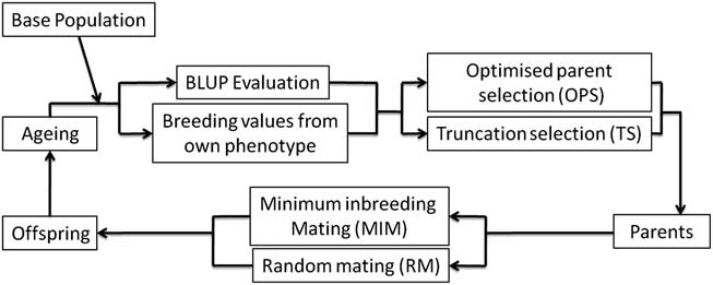
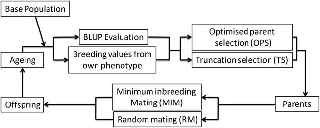
The research approach used in this study is based on simulation of successive generations of animals available for selection in a breeding programme. Figure 1 shows a schematic overview of the processes that make up the simulation model. In each generation, individuals in the population are evaluated and assigned estimated breeding values, then a set of parents is chosen on the basis of these estimated breeding values to make up the mating pairs for the next generation. These mating pairs are chosen and a set of offspring is generated for each pair. Each individual can only be selected as a parent once, which is realised in the simulation by associating chosen parents with a qualifier that eliminates them from being chosen again.
Schematic overview of the processes making up the simulation model. BLUP = best linear unbiased prediction.
Base population
A base population was generated with equal numbers of unrelated males and females expressing a single trait with a heritability (h 2) of 0.3. True breeding values (TBV) for animals in the base population were simulated from a random normal distribution with a standard deviation equal to the square root of the trait heritability. Phenotypes were obtained by adding a simulated random environmental effect to the TBV:
 $$P\, = \,{{\delta }_1}\sqrt {{{h}^2} } \sqrt {\sigma _{p}^{2} } \, + \,{{\delta }_2}\sqrt {(1\,{\rm{ - }}\,{{h}^2} )} \sqrt {\sigma _{p}^{2} } $$
where δ 1 and δ 2 are random deviates sampled from a standard normal distribution (with a mean of zero and a standard deviation of 1). Results can easily be rescaled to a phenotypic standard deviation for any trait or index of interest. Simulations were restricted to a heritability of 0.3, with the exception of the scenarios that considered common environmental effects (details below). This reflects a single trait of moderate heritability suitable for mass selection in a new breeding programme for a species relatively new to aquaculture.
Selection
Two methods were used for parent selection (Figure 1), an optimised and a non-optimised method. Under the non-optimised truncation selection (TS) method, the animals eligible to be parents were sorted by descending phenotype (raw trait data) and the top n females and n males were selected as the parents for the next generation of offspring. No attention was paid to the relatedness of the selected individuals. This method provides a baseline to allow comparison of the effectiveness of selecting parents using an OPS method. It is also a simple and practical method to implement under mass selection, with no knowledge of the ancestry of selection candidates being required.
There may be scope in mass selection aquaculture breeding programmes to use optimum contributions and manage contributions of parents to gamete pools, but when specific family pairings are required at mating, it is not expected to be practical to mate parents such that contributions to future generations are deliberately higher for some parents than others (Skaarud et al., Reference Skaarud, Woolliams and Gjøen2011). Thus, we have restricted the situations simulated in this study to situations where parent pairs selected using an optimisation algorithm contribute equally to the pool of offspring that become selection candidates for the next generation.
For the optimised method in this study, semi-definite programming (Pong-Wong and Woolliams, Reference Pong-Wong and Woolliams2007) was used to identify a set of parents that maximise genetic response for a selection criterion while constraining average relatedness among selected parents as defined by the coefficient of relationship (Wright, Reference Wright1922) to a 1% increase per generation. In this system, it is assumed that a pool of high performing selection candidates are matched to their parents using a DNA parentage system. The semi-definite programming algorithm returns a vector of assigned contributions for the selection candidates. In order to force the algorithm to select a set of n parents that will go on to contribute equally to the new generation and meet the constraint on inbreeding, the contributions of selected parents were effectively fixed by applying a maximum contribution constraint for all potential parents of 1/n, where n is the total number of parents desired. As the sum of the parent contributions is constrained to equal one in the semi-definite design, this constraint ensures that never fewer than n parents will be selected. If more than n parents are given non-zero contributions in the semi-definite solution, then the individuals with the largest n contributions are selected. A further constraint was applied to ensure that equal numbers of male and female parents are selected. It was necessary to add the constraint on parental contributions as early testing of the method returned very small numbers of parents with large contributions in the early generations that still met the co-ancestry constraint. This was not of practical use as it resulted in little genetic diversity for use in later generations.
All parents were selected from the base population in generation zero, and subsequently from individuals generated from the previous round of matings (i.e. non-overlapping generations). The selection criteria were either phenotypic trait values or BLUP predictors of genetic merit. Under the OPS method, the number of individuals ranking highest for the selection criterion that were submitted to the optimisation process was normally limited to four times the number of parents needed. In practice, it is highly unlikely that any fish ranked below this cut-off point could improve the OPS solution.
Initial simulations identified that in some situations with small numbers of parent pairs and or where tight constraints on the rate of accumulation of co-ancestry were applied, the method of OPS was unable to find a feasible set of parents from the 4n selection candidates available. Consequently, a two-step method was developed to find a solution. The first step was based on the concept of walk-back selection (Doyle and Herbinger, Reference Doyle and Herbinger1994). Successive increments of the next highest ranking 50 individuals for the selection criterion (raw phenotype) were added as candidates for consideration by the OPS algorithm. In practice, these fish would also require DNA verification of their parentage, in addition to the 4n selection candidates already considered for OPS. If the method was unable to find a feasible set of parents after the addition of four sets of 50 parentage matched individuals, the second step was to relax the constraint on the percentage increase in co-ancestry per generation. A binary search algorithm was used to find the smallest possible increase in the inbreeding constraint that would allow the OPS method to find a feasible set of parents. The search method takes the current generation constraint and searches increasingly smaller intervals to find the smallest possible increase in the constraint that will allow a feasible solution. Both steps of relaxation were independent across generations in a replicate, so the inbreeding constraint and candidate selection pool size reverted to the standard values (i.e. a 2ΔF% increase in co-ancestry and a selection pool of 4n candidates) for the next generation after relaxation.
Mating
Two alternate methods were used for mate allocation (Figure 1): random mating (RM) and MIM. With both mating schemes, either a single parent pair (1 × 1) mating design or a 2 × 2 cross design was employed. With a 2 × 2 cross design, every male parent is assigned to be mated to two different females and every female is mated to two different males, and the matings are chosen independently so the two males will not be mated to the same two females. Partial factorial mating designs, of which 2 × 2 designs are a practical example, have been shown to result in higher accuracy and precision in genetic parameter estimates when compared with full factorial and nested mating designs in fish (Berg and Henryon, Reference Berg and Henryon1998). Under RM, the selected parents were randomly assigned to mating pairs to ensure each individual is a member of either one or two mating pairs, depending on the design. Under MIM, integer programming was used to identify the set of parent matings that minimised the average level of co-ancestry among all mating pairs, under the 1 × 1 or 2 × 2 mating design constraint. An objective function where the objective coefficients corresponded to the co-ancestry of all possible mating pairs was minimised. Each possible mating pairing was constrained to be either one or zero, that is, selected or not selected as a mating pair, respectively. Additional constraints limited the number of parent pairs to fit the 1 × 1 or 2 × 2 cross designs described above.
Simulation of offspring
Equal numbers of offspring were simulated for each unique parent mating pair. True breeding values (TBVo) for 100 offspring per parent pair were simulated as a function of male (TBVm) and female (TBVf) parent TBV and a Mendelian sampling term as follows:
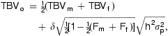 $${TB{{V}_o}\, = \,\tfrac{1}{2}(TB{{V}_m}\, + \,TB{{V}_f})\, \cr \quad+ \,\delta \sqrt {\tfrac{1}{2}[1\,{\rm{ - }}\,\tfrac{1}{2}({{F}_m}\, + \,{{F}_f})]} \sqrt {{{h}^2} \sigma _{p}^{2} }, $$
where δ is a random deviate sampled from a standard normal distribution (with a mean of zero and a standard deviation of 1), Fm and Ff are the inbreeding coefficients of the sire and dam, respectively, and h 2 is the heritability of the trait under selection with phenotypic variance  $$)(-->$<>\sigma _{p}^{2} <$>
<!--$$ . Phenotypes for each offspring were simulated by multiplying a random deviate sampled from a standard normal distribution by the residual standard deviation term
 $$)(-->$<>\scriptstyle{\sqrt {(1\,{\rm{ - }}\,{{h}^2} \,{\rm{ - }}\,{{c}^2} )\sigma _{p}^{2} } <$><!--$$ and adding this and a common environmental effect for each family to the TBVo. The term c 2 gives common environmental effect variance as a proportion of phenotypic variance. Common environmental effects were equal for all individuals within a full-sib family, and were computed by multiplying a random deviate sampled from a standard normal distribution by the standard deviation of common environmental effects,
 $$)(-->$<>\scriptstyle{\sqrt {{{c}^2} \sigma _{p}^{2} } <$>
<!--$$.
For the majority of scenarios, values of c 2 = 0, h 2 = 0.3 and  $$)(-->$<>\sigma _{p}^{2} \, = \,1<$>
<!--$$ were applied such that there were no common environmental effects between tanks. However, in fish relatively large estimates of common environmental effects have sometimes been reported (e.g. Winkelman and Peterson, Reference Winkelman and Peterson1994). To test the effect of rearing individual families separately in a hatchery situation, two scenarios of common environmental effects were simulated while all other variables remained fixed. In the first scenario, the non-genetic common environmental effect (c 2) is simulated to substitute a portion of residual variance (e 2) with the non-genetic variance evenly split between c 2 and e 2, so that
 $$)(-->$<>{{c}^2} \, = \,{{e}^2} \, = \,{{(1\,{\rm{ - }}\,\sigma _{a}^{2} )} \mathord{\left/ {\vphantom {{(1\,{\rm{ - }}\,\sigma _{a}^{2} )} 2}} \right. \kern-\nulldelimiterspace} 2}\, = \,0.35<$>
<!--$$ with the additive genetic variance
 $$)(-->$<>\sigma _{a}^{2} <$>
<!--$$ remaining at 0.3, giving h 2 = 0.3 if we have a phenotypic variance of one. This implies that the management practice that leads to a common environmental effect does not generate any additional environmental variance. In the second scenario, c 2 is simulated to be additive to e 2 and a 2with c 2 = e 2 and the additive genetic variance c 2 remaining at 0.3 giving h 2 = a 2/(a 2 + c 2 + e 2) = 0.3/(0.3 + 0.7 + 0.7) = 0.18. In this case, the genetic variance is unchanged, but the combined environmental variance is increased.
BLUP evaluation
For the majority of scenarios simulated, raw phenotype was used as the selection criterion. For some situations, BLUP evaluation using ASREML software (Gilmour et al., Reference Gilmour, Cullis, Welham and Thompson1999) was simulated to incorporate information from relatives into selection decisions. Because year effects are expected to exist in practice, year class was fitted as a sole fixed effect adjustment factor in a univariate animal model analysis to account for uncertainty in year adjustment when incorporating information from relatives in other years when predicting merit of a candidate using BLUP. No year effects were simulated because no selection was carried out across years. The true heritability and phenotypic standard deviation from the simulation were used to parameterise the BLUP evaluation.
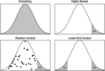
In practice, identification of the parents of all potential selection candidates by genotyping may be expensive, and or impractical. To further test the robustness of BLUP breeding values as the selection criterion for OPS, we simulated the effects of both (i) not knowing the true parents of varying proportions of selection candidates, and also of (ii) not considering the phenotypic records of animals without pedigree in the genetic evaluation process. Figure 2 illustrates the levels of known pedigree data in the generation of BLUP breeding values for the various situations. For the scenario labelled ‘Everything’, all selection candidates have known pedigree. Scenarios were compared where only the top 5% of animals by raw trait data had known parents (‘Highly Biased’) with alternate situations where another 5% with known parents were randomly chosen (‘Random Control’) or where the top 5% and the bottom 5% based on unadjusted trait phenotypes had known parents (‘Lower End Control’).
Levels of known pedigree data used in the simulations where the selection criterion was Best Linear Unbiased Prediction (BLUP) breeding values.

Variation of parameters
All simulations ran 25 replicates of 15 generations of selection and mating. Average breeding values, average inbreeding coefficients and average relationships among all offspring were computed by generation for the population created in each replicate. Results for all 25 replicates were averaged by generation. Standard errors were also computed to provide a confidence interval to test for statistically significant differences between designs. The means over all the replicates for each generation were compared between scenarios where one variable was changed. An unpaired t-test was used to test for significant differences between TBV and average inbreeding results in comparable scenarios.
Initial scenarios compared the OPS and TS methods of selection when combined with MIM and RM in a 1 × 1 mating design with 30 parents of each sex. The effect of using 1 × 1 and 2 × 2 mating designs with three levels of common environmental effect was tested with OPS and MIM and 30 families. These scenarios led to a narrowed focus on using OPS with MIM and 1 × 1 mate design in a range of scenarios designed to model small breeding programmes. The initial mating designs that were evaluated had from 30 to 200 parents of each sex and resulted in 30 to 200 full-sib families with the one by one mating design. The constraint on maximum co-ancestry among parents in the optimised method of parent selection was set at a range of alternative values between 1% and 4% increase per generation in scenarios with MIM and a 1 × 1 mate design. In other scenarios walk-back selection was experimented with when there were very small numbers of parents and the OPS method was unable to meet the relatedness constraint. Breeding programmes with 5, 15 and 30 full-sib families were therefore simulated to test the ability of the OPS method to find a set of parents to meet the constraint on relatedness. Each of these scenarios were run twice, where walk-back selection was only allowed if the OPS method was unable to meet the constraint on relatedness. Scenarios using BLUP breeding values as selection criteria in the OPS method had 30 families and used the MIM method with a 1 × 1 mate design; these scenarios varied in the amount of information available in the BLUP evaluation. In all scenarios, each full-sib family produced 100 offspring with equal sex ratio simulated as being reared communally, with the exception of the scenarios investigating the effect of a common environmental effect where the families were simulated as being reared separately.
Genetic gain was measured by the change in the average TBV of the population at each generation, in units of a phenotypic standard deviation. Inbreeding was calculated using the algorithm described by Meuwissen and Luo (Reference Meuwissen and Luo1992) and has been reported as the average inbreeding coefficient of individuals by generation. Average co-ancestry among all offspring within a generation was also computed using the algorithm described by Meuwissen and Luo (Reference Meuwissen and Luo1992). Average inbreeding has mainly been reported in results because the focus of this paper is on small breeding programmes in new aquaculture industries where there are long generational intervals, and thus actual inbreeding estimates provide a better statistic to compare between schemes.
Results
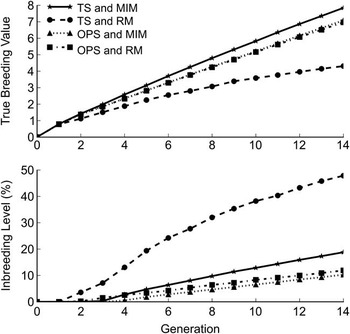
Figure 3 shows a comparison of genetic response and average inbreeding of all simulated offspring by generation for a situation where there are 30 families when comparing the two types of parent selection (MIM and RM) and the two types of mate allocation (OPS and TS) with a 1 × 1 mating design. No common environmental effects were simulated and the heritability was 0.3 with an inbreeding constraint of 1% increase per generation for OPS.
Average true breeding value (standard deviations) and inbreeding level (%) over 15 generations when the parents are selected by either optimal parent selection (OPS) or truncation selection (TS) and mate allocations are by minimum inbreeding mating (MIM) or random mating (RM).

As there is no constraint on inbreeding in the TS + RM scenario, the rapid increase in inbreeding starts to affect the genetic progress considerably after only five generations when compared with other scenarios that use either OPS, MIM or both (Figure 3). The use of the OPS method achieved a lower TBV by the 15th generation when compared with the use of TS to select the parents (Figure 3) when MIM was used to assign mating pairs. However, the inbreeding levels for the two OPS treatments were substantially lower than for the two TS treatments.
MIM also increased inbreeding percent at a slower rate compared with RM (Figure 3), but differences in TBV after 15 generations were not statistically significant (Table 1). MIM delayed the onset of inbreeding by approximately one generation. OPS did not delay the onset of inbreeding, but lead to a slower increase in inbreeding levels in generations three to 15. The inbreeding level of the OPS with the MIM scheme was less than a quarter of the inbreeding level at the 15th generation of the scenario where TS and RM were used.
Average genetic response in phenotypic standard deviations (standard errors) and inbreeding level (%) at 5, 10 and 15 generations for different strategies of parent and mate selection

OPS = optimum parent selection; TS = truncation selection; MIM = minimum inbreeding mating; RM = random mating.
All scenarios had 30 families in a 1 × 1 mate design with h 2 = 0.3, c 2 = 0, a 1% constraint on maximum inbreeding increase per generation and selection on raw phenotype. Each family produced 100 offspring with equal sex ratio.
a–c Within a column, means without a common superscript letter differ (P < 0.05).
Table 1 also shows differences in co-ancestry over time for the different selection and mating strategies. Typically differences across strategies for co-ancestry closely mirrored differences for inbreeding. This was also observed in other simulations and so no further co-ancestry results have been reported.
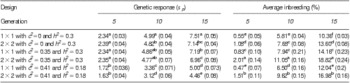
The 2 × 2 and 1 × 1 mating designs were compared at three levels of common environmental effects with both OPS and MIM strategies applied to a breeding programme with 30 families (Table 2). Thus, there were 30 parents of each sex in the 1 × 1 design and 15 parents of each sex in the 2 × 2 design. With no simulated environmental effects there was no significant difference in the genetic progress attained by the designs; however, the 1 × 1 design had significantly lower (P < 0.001) average inbreeding by the 15th generation. The scenario where c 2 = 0.35 with no reduction in heritability resulted in genetic progress that was not significantly different from the scenario where there was no common environmental effect. However, the average inbreeding percentage with both the 1 × 1 and 2 × 2 mating designs was significantly higher (P < 0.001) than the corresponding scenarios with c 2 = 0 by the 15th generation. In contrast, when common environmental variance was simulated as an additional component to the genetic and residual variance such that c 2 = 0.41 and consequentially h 2 = 0.18, genetic responses with 1 × 1 and 2 × 2 mating designs were significantly lower (P < 0.001) than the corresponding scenarios where h 2 = 0.3. Genetic progress in the 2 × 2 mating design was not higher than in the 1 × 1 design for any of the scenarios with common environmental effects, whereas average inbreeding was always significantly higher after 5, 10 and 15 generations of selection.
Average genetic response in phenotypic standard deviations (standard errors) and inbreeding level (%) at 5, 10 and 15 generations with the comparison of the 1 × 1 and 2 × 2 mating designs with varying degrees of common environmental effects

OPS = optimum parent selection; MIM = minimum inbreeding mating.
All scenarios had 30 families using OPS and MIM with selection on raw phenotype with h 2 = 0.3, c 2 = 0 and a 1% constraint on maximum inbreeding increase per generation. Each family produced 100 offspring with equal sex ratio.
a–fWithin a column, means without a common superscript letter differ (P < 0.05).
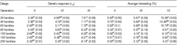
Table 3 shows a comparison between scenarios of the genetic response and average inbreeding results of all simulated offspring by generation for numbers of parents (equal for each sex) selected each generation varying from 40 to 200 with both OPS and MIM in a 1 × 1 mating design. Increasing the number of families from 60 to 80 in the breeding programme resulted in significantly higher genetic progress over the 15 generations with significantly lower inbreeding levels (Table 3). When the number of families exceeded 60, the addition of further families led to a significant (P < 0.001) decrease in the inbreeding level by the 15th generation. With 150 families, the initial increase in inbreeding levels was delayed until around the fifth generation, and the inbreeding level had a much slower rate of increase per generation compared with when there were 40 to 60 families.
Average genetic response in phenotypic standard deviations (standard errors) and inbreeding level (%) at 5, 10 and 15 generations with varying number of families in a 1 × 1 mating scheme using OPS and MIM for parent and mate selection with h 2 = 0.3, c 2 = 0, a 1% constraint on maximum inbreeding increase per generation and selection on raw phenotype. Each family produced 100 offspring with equal sex ratio

OPS = optimum parent selection; MIM = minimum inbreeding mating.
a–f Within a column, means without a common superscript letter differ (P < 0.05).
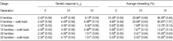
With five families per generation, the OPS method was unable to meet the constraint on relatedness, regardless of whether or not walk-back selection was used. For this structure, inbreeding levels reached around 38% by the 15th generation, compared with just over 10% for the situation where there were 30 parents of each sex (Table 4). Although genetic progress was ∼17% lower with 15 families than it was with 30 families, on average the rate of increase in inbreeding was still within tolerable limits for short-term management of a population. There were no significant differences between the results for each scenario with and without the inclusion of the walk-back option for when relatedness does not reach the target constraint.
Average genetic response in phenotypic standard deviations (standard errors) and inbreeding level (%) at 5, 10 and 15 generations with small families with the option of using walk-back to increase the size of the selection pool for OPS if the co-ancestry constraint cannot be met initially

OPS = optimum parent selection; MIM = minimum inbreeding mating.
All scenarios used OPS and MIM for parent and mate selection with h 2 = 0.3, c 2 = 0, a 1% constraint on maximum inbreeding increase per generation and selection on raw phenotype. Each family produced 100 offspring with equal sex ratio.
a–d Within a column, means without a common superscript letter differ (P < 0.05).
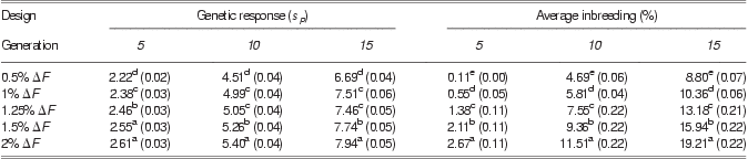
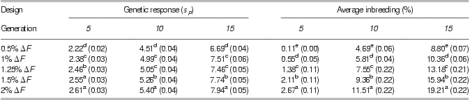
Table 5 shows results from scenarios where the relatedness constraint was varied from a 0.5% increase per generation to 2% with OPS and MIM and a 1 × 1 mating design with 30 families. The average inbreeding percentage at generation 15 for the 0.5% constraint is significantly lower (P < 0.001) than the 1% constraint showing that with 30 families in a 1 × 1 mating design it is possible to restrict the inbreeding increase to a 0.5% increase per generation, however, this led to a significantly lower (P < 0.001) genetic gain level by generation 15. Increases in genetic gain with a rate of inbreeding constraint above 1% per generation were modest.
Average genetic response in phenotypic standard deviations (standard errors) and inbreeding level (%) at 5, 10 and 15 generations with variation of the constraint on the maximum inbreeding increase per generation in a 1 × 1 mating scheme with 30 families using OPS and MIM for parent and mate selection with h 2 = 0.3, c 2 = 0. Each family produced 100 offspring with equal sex ratio
OPS = optimum parent selection; MIM = minimum inbreeding mating.
a–e Within a column, means without a common superscript letter differ (P < 0.05).
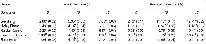
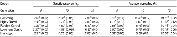
Table 6 shows a comparison of genetic response and average inbreeding of all simulated offspring by generation for 30 parents of each sex and different levels of pedigree data in the generation of BLUP breeding values with OPS and MIM in a 1 × 1 mating scheme. The scenario where all pedigree data were known produced the highest level of genetic response, but this scenario also had the highest level of inbreeding observed at the 15th generation. These high levels of inbreeding indicate that the OPS selection was unable to meet the desired constraint on inbreeding. The genetic response levels for the simulations where a proportion of the pedigree data were simulated as being known were similar over all generations. The ‘Random Control’ and ‘Lower End Control’ scenarios had similar levels of genetic gain and inbreeding to the simulation where selection was based on phenotype.
Average genetic response in phenotypic standard deviations (standard error in brackets) and inbreeding level (%) at 5, 10 and 15 generations with a varying amount of pedigree data available in BV estimation using BLUP
BV = breeding value; BLUP = best linear unbiased prediction; OPS = optimum parent selection; MIM = minimum inbreeding mating; EBV = estimated breeding values.
A 1 × 1 mate design with 30 families using OPS and MIM for parent and mate selection based on EBV, with h 2 = 0.3, c 2 = 0 and a 1% constraint on maximum inbreeding increase per generation. Each family produced 100 offspring with equal sex ratio.
a–d Within a column, means without a common superscript letter differ (P < 0.05).
Discussion
The results clearly demonstrate that small breeding programmes are more feasible with the use of mathematical optimisation tools opening the way for genetic improvement of newly domesticated aquaculture species. In contrast to mathematical optimisation tools BLUP selection only modestly increased the rate of genetic response for the simulated trait, while at the same time giving a substantial increase in the rate of inbreeding.
In general, use of different breeding programme sizes and strategies had a larger effect on the levels of inbreeding than on the rate of genetic gain. The OPS algorithm still chose the parents with the best phenotype values possible, but with fewer than 30 families it was much more likely to push the boundary of the constraint on relatedness in the selection of these parents as there was less genetic variation in the pool of selection candidates, whereas with more than 30 families the resulting increase in co-ancestry from selecting the best families may be lower than the constraint. As the number of parents of each sex increased, there was more genetic variation in the pool of selection candidates, as they come from more families, and also a larger number of parents available in the MIM to assign mating pairs that do not lead to inbred offspring.
Although having a larger number of families decreased inbreeding, in practical situations the number of families almost always will be a significant limiting factor due to biological, physical and cost constraints on the number of spawning parent brood stock available, as well as the size and number of tanks and the costs of rearing and evaluating the families (Coman and Henshall, Reference Coman and Henshall2010; Masuma et al., Reference Masuma, Takebe and Sakakura2010). In particular, the similarity in levels of genetic gain across varying numbers of families is of interest as it showed that meeting the relatedness constraint with smaller numbers of families only requires a trade-off with lower levels of genetic gain when numbers of families are low (i.e. below 30 families with a 1 × 1 mating structure).
Several studies have considered the effects of different mating designs on genetic response and inbreeding in aquaculture breeding programmes. Doyle and Herbinger (Reference Doyle and Herbinger1994) used DNA based matching of selection candidates to their parents in a walk-back selection method to avoid rearing families separately until tagging size. Walk-back identifies only enough individuals for parentage testing to reach a desired level of genetic diversity among the finally selected individuals. Blonk et al. (Reference Blonk, Komen and van Arendonk2010) showed that genotyping the top 5% to 10% of candidates and then performing optimal contribution selection will allow restriction of the increase in the levels of inbreeding to be maintained at 1% per generation. Herbinger et al. (Reference Herbinger, Doyle, Pitman, Paquet, Mesa, Morris, Wright and Cook1995) used walk-back selection in the analysis of paternal and maternal effects on offspring growth and survival in rainbow trout. This allowed high selection intensities with a minimal increase in inbreeding. When walk-back selection was simulated in the present study for situations with very small numbers of parents (five to 30 parents of each sex) and in the absence of common environmental effects, there were minimal benefits. One explanation of this observation is that because of the small number of families present, most were already sampled in the first pool of individuals identified as selection candidates for parentage matching. Walk-back systems would likely offer greater benefits when the original pool of candidates selected for parentage matching was small and genotyping additional candidates is likely to identify more families, and where heritability and/or common environmental effects are large. In these situations, walk-back selection would provide a less related pool of candidates allowing the OPS algorithm to select a set of parents to meet the constraint on relatedness.
The absence of substantive benefits through BLUP genetic evaluation in the situations simulated in this study supports earlier conclusions by Belonsky and Kennedy (Reference Belonsky and Kennedy1988). The results in this study from the scenarios where a portion of the data missing in the BLUP evaluation showed similar results to the simulation work by Dupont-Nivet et al. (Reference Dupont-Nivet, Haffray and Vandeputte2010). Estimated breeding values generated by BLUP can be highly biased when part of the pedigree data is unknown in a population containing large full-sib groups if the known pedigree corresponds to a selected sub sample. Under optimum parent selection, exploitation of between-family differences in estimated genetic merit is moderated to control inbreeding. The superiority over phenotypic selection of genetic evaluation techniques such as BLUP that increase the use of between-family information is therefore moderated under OPS. For the same reason, the effects of biases in estimates of family differences in merit such as with BLUP on selected data are also moderated.
Hatchery techniques to manage environmental effects could be required in order to facilitate equal contributions of full-sib families to future selection candidates, or for offspring to reach sufficient size for individual tagging. Under both the 1 × 1 and 2 × 2 mating designs, the presence of common environmental effects either reduced response to selection or increased inbreeding, depending on the way they were manifested. However, our results showed that the 1 × 1 mating design performed better, with lower levels of average inbreeding after 15 generations for a similar level of genetic progress, at each of the simulated levels of common environmental effect. In the 1 × 1 mating design we have twice as many parents to form the same number of families, compared with a 2 × 2 design. It is therefore likely that more genetic variation exists in the parents selected.
For the small breeding programmes addressed here, managing genetic diversity needs to be a primary driver of breeding scheme design. The results of this study demonstrate that within-family selection is the main contributor to genetic progress under these circumstances. Thus, with a small breeding programme, it could in some instances be preferable to accept the creation of common environmental effects on full-sib families through careful separate rearing at early life stages, if this means more uniform survival of offspring across parent pairings. In this way, the maintenance of genetic diversity contributed by all of the individuals selected to become parents would be maximised.
With 2 × 2 designs, more statistical power is achieved to partition full-sib family genetic effects from common environmental effects (Berg and Henryon, Reference Berg and Henryon1998). This would be useful in new breeding programmes where knowledge of both genetic parameters and the magnitude of common environmental effects are limited. One further advantage of the 2 × 2 design is that separate breeding values can be better estimated for each parent in the pair. The family performance gets equally attributed to each parent in a 1 × 1 mating design, and so two parents with potentially quite different genetic merit will finish up with very similar estimated breeding values. With high reproductive rates in aquaculture, progeny tested parents with accurate breeding values could be useful in generating large numbers of superior commercial fish quickly, and so having better separation of predictions of merit of parents could also be an advantage. Factorial designs with higher densities in the off diagonals lead to reductions in inbreeding if rearing and mating resources for specific full-sib groups are unlimited (Leitch et al., Reference Leitch, Smith, Burnside and Quinton1994; Dupont-Nivet et al., Reference Dupont-Nivet, Vandeputte, Haffray and Chevassus2006), but when the number of full-sib families is constrained, factorial designs result in a smaller effective population size and hence much higher rates of inbreeding.
Bentsen and Olesen (Reference Bentsen and Olesen2002) considered the design of mass selection programmes with TS and RM and recommended at least 50 mating pairs of individuals be established with the number of progeny tested per pair standardised to be not less than 30 to 50. In this study, we have found that OPS and MIM can facilitate breeding designs with smaller numbers of parents selected (i.e. 15 parents of each sex) that meet acceptable rates of realised inbreeding over seven to 15 generations. These smaller breeding scheme designs would have the advantage of much lower costs in particular for situations where separate mating and/or rearing of full-sib families is required.
We have assumed that in each generation, all mating pairs produce an equal number of surviving offspring. This is commonly unrealistic in practice, as observed in gilthead sea bream (Brown et al., Reference Brown, Woolliams and McAndrew2005) and Coho salmon (Gallardo et al., Reference Gallardo, Lhorente and Neira2010), because of the limited ability to control and manipulate spawning and often unpredictable fertilisation rate and egg/larval survival (Garber et al., Reference Garber, Tosh, Fordham, Hubert, Simpson, Symonds, Robinson, Bowman and Trippel2010). It is well known that unequal family size reduces effective population size (Falconer and Mackay, Reference Falconer and Mackay1996), for example, in gilthead sea bream (Brown et al., Reference Brown, Woolliams and McAndrew2005) and Atlantic cod (Garber et al., Reference Garber, Tosh, Fordham, Hubert, Simpson, Symonds, Robinson, Bowman and Trippel2010). Future simulation work should take account of variation in the number of offspring produced by mating pairs (e.g. Blonk et al., Reference Blonk, Komen and van Arendonk2010) and evaluate group spawning designs where multiple parents are mated together in large spawning tanks. This would be relevant for large marine finfish, where it is impractical to manage individual mating pairs at spawning.
Conclusion
Under the mating designs simulated here and with equal contributions by family pairs to the next generation of parents, we conclude that 15 parents of each sex that successfully reproduce is a minimum breeding programme size to be confident of achieving sustainable rates of genetic progress without excessive inbreeding. To achieve this, inbreeding management tools such as OPS and MIM are required. In many applied situations, especially for new aquaculture species, the cost and practicalities associated with using these tools are likely to be much less onerous than those associated with selecting and individually mating and rearing much larger numbers of parents. The utilities of BLUP selection are shown to be limited with a small pool of selection candidates due to increases in inbreeding when selection is for a single trait only. For small breeding programmes, common environmental effects associated with full-sib families are not very problematic, because the majority of selection must be applied within families to meet the inbreeding constraint.
Acknowledgements
Funding for this research was provided by the Ministry of Science and Innovation.