1. Introduction
One of the most peculiar aspects of turbulence in wall-bounded flows is the ability of the turbulent fluctuations to regenerate themselves through self-sustained processes. In wall flows, the production of turbulent fluctuations is embedded in the system instead of being provided by an external agent. The dynamics of these self-sustaining mechanisms has been extensively investigated over the past 30 years, since these processes are responsible for the energy drain from the mean flow to the fluctuating field and for the turbulent drag.
It has long been understood that the near-wall layer, being the site of the highest rate of turbulent energy production and of the maximum turbulent intensities, is crucial to the dynamics of attached shear flows. The possibility to identify robust kinematic features in the proximity of a wall fed the hope of the scientific community to obtain a complete and consistent dynamical description of the underlying physics of these processes. The turbulent fluctuations near a wall have been found to organize in well-defined coherent motions consisting of quasi-streamwise vortices and high/low-velocity regions alternating in the spanwise direction. The former are longitudinal vortices with typical streamwise and spanwise length scales
 ${\it\lambda}_{x}^{+}\approx 200$
and
 ${\it\lambda}_{z}^{+}\approx 50$
, respectively (hereafter a superscript
 $+$
will denote the so-called inner units; see e.g. Townsend Reference Townsend1976), slightly tilted away from the wall. The latter are long and wide alternating arrays of streamwise streaks of local velocity excess/defect, with length scales
 ${\it\lambda}_{x}^{+}\approx 1000$
and
 ${\it\lambda}_{z}^{+}\approx 100$
, superimposed on the mean flow. These features have been recognized in several numerical and experimental works (see e.g. Kim, Kline & Reynolds Reference Kim, Kline and Reynolds1971; Smith & Metzler Reference Smith and Metzler1983; Robinson Reference Robinson1991). From these observations, several scientists tried to derive a conceptual model of these processes. Following the work of Jiménez & Pinelli (Reference Jiménez and Pinelli1999), the continuous creation and destruction of these turbulent structures form a self-sustaining cycle maintaining near-wall turbulence without the need of any input from the core flow, i.e. it is an autonomous cycle. The streamwise vortices extract energy from the mean flow to create alternating streaks of longitudinal velocity. Presumably by inflectional instabilities, these streaks in turn give rise to the vortices closing the cycle (see also Hamilton, Kim & Waleffe Reference Hamilton, Kim and Waleffe1995; Jeong et al.
Reference Jeong, Hussain, Schoppa and Kim1997; Schoppa & Hussain Reference Schoppa and Hussain2002).
From a more applied point of view, the near-wall cycle is crucial, since it controls the magnitude of the wall stress. But coherent structures exist also at larger scales in the so-called overlap layer (Hutchins & Marusic Reference Hutchins and Marusic2007a ,Reference Hutchins and Marusic b ; Jiménez & Hoyas Reference Jiménez and Hoyas2008), and have recently been suggested to form an outer self-sustaining mechanism of regeneration of very large turbulent fluctuations (see e.g. Flores & Jiménez Reference Flores and Jiménez2006; Hwang & Cossu Reference Hwang and Cossu2010; Mizuno & Jiménez Reference Mizuno and Jiménez2013). The phenomenology resembles the self-regenerating cycle near the wall though its characteristic dimensions are larger (see e.g. del Alamo et al. Reference del Alamo, Jiménez, Zandonade and Moser2006; Monty et al. Reference Monty, Stewart, Williams and Chong2007). The coherent motions involved in this outer cycle should scale with external variables, meaning that their dimensions and action should increase as the extent of the log layer widens with Reynolds number. Hence, the understanding of these outer dynamics is crucial for the modelling of wall turbulence in the asymptotic regime of very large Reynolds number. Furthermore, its analysis could help to clarify the interactions between the outer and inner regions of wall flows needed in the formulation of near-wall models for large-eddy simulations (see e.g. Piomelli & Balaras Reference Piomelli and Balaras2002), and to explain the controversial mixed inner/outer scaling of the near-wall quantities such as spectra and turbulent intensities (see e.g. Hutchins & Marusic Reference Hutchins and Marusic2007b ; DeGraaff & Eaton Reference DeGraaff and Eaton2000).
Generally speaking, the problem of wall turbulent flows has been classically studied by dividing the flow domain into well-characterized regions depending on wall distance. In particular, wall-bounded flows are divided into a near-wall inner region and an outer region populated by large structures. These two distinct regions are present in all wall-bounded flows and interact in the overlap region. While in the outer flow the velocity profile depends on the particular flow configuration, in the inner and overlap regions it exhibits a high degree of universality starting linearly from the wall and then approaching a logarithmic behaviour. These behaviours opportunely scaled with viscous units should collapse for different flows and different Reynolds numbers; see Nagib & Chauhan (Reference Nagib and Chauhan2008) for a detailed description of the controversies on this topic. The same scaling should apply to the turbulent intensity profiles and to all the statistical observables of the inner region.
However, the near-wall quantities exhibit a Reynolds-number dependence as shown by the fact that the energy of the long turbulent fluctuations of the overlap layer grows when the Reynolds number increases. This large-scale motion is found to actively modulate the near-wall turbulence by production of near-wall scales at increasing Reynolds number (Hutchins & Marusic Reference Hutchins and Marusic2007b
). The observed increase of the streamwise turbulent fluctuation peak, the possible appearance of a second peak in the overlap flow and the presence of a marked outer-scale peak in the energy spectrum are thought to be a signature of these effects. An important consequence of the Reynolds-number dependence of the large turbulent motion in the overlap layer is that most of the turbulence production should asymptotically come from this region owing to the widening of the overlap layer with
 $\mathit{Re}$
(Smits, McKeon & Marusic Reference Smits, McKeon and Marusic2011). Even if no Reynolds-number dependence for the outer turbulent production intensity is expected, the outer turbulent self-sustained mechanisms are thought to dominate the high-Reynolds-number asymptotic state of wall turbulence.
Given the Reynolds-number dependence of these processes in the compound scale/physical space, an interesting approach to study the basic mechanisms of the outer cycle has recently been proposed in Cimarelli, De Angelis & Casciola (Reference Cimarelli, De Angelis and Casciola2013) by extending the statistical approach used in Marati, Casciola & Piva (Reference Marati, Casciola and Piva2004) and applied by Saikrishnan et al. (Reference Saikrishnan, De Angelis, Longmire, Marusic, Casciola and Piva2012) to moderately high-Reynolds-number data. The classical approach for addressing these issues in channel flow is based on a Fourier decomposition along the homogeneous directions while keeping a description in terms of the physical distance in the wall-normal direction (see e.g. del Alamo et al. Reference del Alamo, Jiménez, Zandonade and Moser2004). However, this more traditional approach does not allow for a net distinction between position in the wall-normal direction and wall-normal scale at which energy generation and energy flux take place. The tool used here to describe the energy content associated with a given scale of motion in a given position in space is based, instead, on the generalization of the Kolmogorov equation for the second-order structure function, originally introduced for homogeneous and isotropic turbulence, and successively extended to inhomogeneous anisotropic flows by Hill (Reference Hill2002). The generalized Kolmogorov equation keeps the two concepts of wall-normal position and wall-normal scale clearly distinct, thereby allowing one to distinguish between the two associated components of the energy flux. In Cimarelli et al. (Reference Cimarelli, De Angelis and Casciola2013), this multidimensional description of turbulence has been used and proven fundamental for the understanding of the wall turbulent physics and for its modelling as shown in Cimarelli & De Angelis (Reference Cimarelli and De Angelis2011). In the present paper, we extend this work by analysing how the turbulent energy associated with a certain scale (scale energy) is generated, transferred and dissipated among different scales and wall distances on varying the Reynolds number, with particular attention being paid to the outer self-regeneration mechanisms.
2. Direct numerical simulation database and single-point statistics
In the present study, we analyse data of three direct numerical simulations (DNS) of fully developed turbulent channel flow at
 $\mathit{Re}_{{\it\tau}}=u_{{\it\tau}}h/{\it\nu}=550$
,
 $1000$
and
 $1500$
, respectively. Here,
 $u_{{\it\tau}}$
is the friction velocity,
 $h$
the channel half gap width and
 ${\it\nu}$
the viscosity. The simulations were carried out with a pseudo-spectral code using Fourier expansions and dealiasing in the homogeneous directions, and Chebyshev polynomials in the wall-normal direction. Full details of the algorithm can be found in Chevalier et al. (Reference Chevalier, Schlatter, Lundbladh and Henningson2007). The domain size and resolution of the three DNS are given in table 1. Data of the DNS at
 $\mathit{Re}_{{\it\tau}}=550$
and 1000 have already been used for studies of wall turbulence in Cimarelli et al. (Reference Cimarelli, De Angelis and Casciola2013) and Lenaers et al. (Reference Lenaers, Li, Brethouwer, Schlatter and Örlü2012), respectively. Let us mention that the lower resolution adopted for the simulation of the lower-Reynolds-number case at
 $\mathit{Re}_{{\it\tau}}=550$
has been tested and found not to affect the statistical quantities we are analysing in the present work.
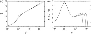
Mean velocity profiles
 $U^{+}(y^{+})$
and (premultiplied) mean velocity gradient
 $y^{+}\text{d}U^{+}/\text{d}y^{+}$
for the three channel DNS considered in this study, with
 $\mathit{Re}_{{\it\tau}}=550$
, 1000 and 1500. Here
 $U^{+}(y^{+})=y^{+}$
and
 $U^{+}(y^{+})=1/{\it\kappa}\log (y^{+})+B$
with
 ${\it\kappa}=0.41$
and
 $B=5.2$
are indicated by thick grey lines.

Parameters of the simulations:
 $\mathit{Re}_{{\it\tau}}$
is the friction Reynolds number;
 $L_{x}$
,
 $L_{y}$
and
 $L_{z}$
are the lengths of the computational domain in the streamwise (
 $x$
), wall-normal (
 $y$
) and spanwise (
 $z$
) directions;
 $N_{x}$
,
 $N_{y}$
and
 $N_{z}$
are the number of points in physical space; and
 ${\it\Delta}_{x}^{+}$
,
 ${\it\Delta}_{y}^{+}$
and
 ${\it\Delta}_{z}^{+}$
are the corresponding grid spacings in viscous units.

Profiles of the streamwise mean velocity and the log-law indicator function of the three DNS are shown in figure 1. The near-wall region has obviously a very high degree of similarity for the three Reynolds numbers, while outside the buffer layer, in the overlap layer, differences due to Reynolds number effects become visible. A tentative plateau in the indicator function profile starts to appear with increasing
 $\mathit{Re}_{{\it\tau}}$
but is not yet clearly present, meaning that a true logarithmic layer is absent even at the highest
 $\mathit{Re}_{{\it\tau}}$
.
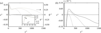
(a) Source term of the kinetic energy budget
 $s^{+}$
(black lines) and corresponding spatial flux
 ${\it\psi}^{+}$
(grey lines) for the three Reynolds numbers
 $\mathit{Re}_{{\it\tau}}=550$
, 1000 and 1500. The inset shows a zoom of the near-wall peak of the spatial flux
 ${\it\psi}^{+}$
. The two arrows indicate increasing Reynolds numbers. (b) Magnification of the region around the second positive peak of
 $s$
. Increasing
 $\mathit{Re}_{{\it\tau}}$
from dash-dotted to dashed and solid lines.

The single-point turbulent kinetic energy balance compacts in a simple way the overall multidimensional behaviour of turbulence describing the energetics only in physical space. For the symmetries of the channel, this equation reads
 $$\begin{eqnarray}\frac{\text{d}{\it\psi}}{\text{d}y}=s(y),\end{eqnarray}$$
and describes how turbulent energy is redistributed among different wall distances
 $y$
through the spatial flux
 ${\it\psi}=(\langle u_{i}^{2}v\rangle +\langle pv\rangle /{\it\rho}-{\it\nu}\text{d}\langle u_{i}^{2}\rangle /\text{d}y)$
from the production to the dissipation regions of the flow defined by positive and negative values of the source term
 $s(y)=-\langle uv\rangle (\text{d}U/\text{d}y)-\langle {\it\epsilon}\rangle$
. Hereafter,
 $\langle \cdot \rangle$
will be used to denote ensemble average. As shown by the black lines in figure 2(a), in wall turbulence the energy source is near the wall in the so-called buffer layer. In this layer, turbulence production exceeds the local dissipation. Conversely, the wall and bulk flow behave as sink regions dissipating turbulent energy emerging from the buffer layer through the spatial energy flux; see grey lines in figure 2(a). Indeed, the spatial flux is zero at the peak of the energy source and becomes positive (towards the core flow) further away from the wall and negative (towards the wall) closest to the wall. Actually, in between the buffer layer and the core of the flow, a third region can be defined, the so-called overlap layer, which is the main subject of the present work. Although this region is expected to be an equilibrium layer where production and dissipation locally balance, production is actually larger than dissipation, leading to an outer energy source; see figure 2(b). The understanding of this region of the flow is very important especially when dealing with the high-Reynolds-number state of wall turbulence. Even if its intensity is very small compared to the one near the wall, this outer energy source shows an apparent
 $\mathit{Re}$
dependence; see again figure 2(b). In particular, it appears that, by increasing the Reynolds number, the role of the outer energy source becomes more important. By defining the overall inner and outer energy source as the integral of the source
 $s(y)$
restricted to the two (inner and outer) regions where
 $s(y)>0$
, respectively,
 $$\begin{eqnarray}\displaystyle {\it\Xi}_{inn}=\int _{y}s(y)\text{d}y\quad y\in \{\text{inner region of energy source}\;s(y)>0\}, & & \displaystyle \nonumber\\ \displaystyle {\it\Xi}_{out}=\int _{y}s(y)\text{d}y\quad y\in \{\text{outer region of energy source}\;s(y)>0\}, & & \displaystyle \nonumber\end{eqnarray}$$
we can roughly estimate the relative importance of the two regions as a function of Reynolds number by means of the ratio
 ${\it\Xi}_{out}/{\it\Xi}_{inn}$
. The present data show a significant increase of this ratio from
 $0.0031$
at
 $\mathit{Re}_{{\it\tau}}=550$
to
 $0.0347$
and
 $0.0617$
at
 $\mathit{Re}_{{\it\tau}}=1000$
and
 $1500$
, respectively. Extrapolating this trend, one can expect the outer source to become dominant above
 $\mathit{Re}_{{\it\tau}}=15\,000{-}20\,000$
. The increased intensity of the outer source also has consequences for the topology of the energy transfer. Indeed, as shown in figure 2(a), the spatial flux in the overlap layer increases with
 $\mathit{Re}$
and forms an outer peak given by the increasing energy injection due to the outer energy source.
3. Generalized Kolmogorov equation
The generalized Kolmogorov equation proposed by Hill (Reference Hill2002) is the balance equation for the second-order structure function,
 $\langle {\it\delta}u^{2}\rangle$
, where
 ${\it\delta}u^{2}={\it\delta}u_{i}{\it\delta}u_{i}$
and the fluctuating velocity increment is
 ${\it\delta}u_{i}=u_{i}(X_{s}+r_{s}/2)-u_{i}(X_{s}-r_{s}/2)$
. According to its definition,
 $\langle {\it\delta}u^{2}\rangle (r_{i},X_{i})$
depends both on the separation vector defined as
 $r_{i}=x_{i}^{\prime }-x_{i}$
and on the location specified by the midpoint
 $X_{i}=(x_{i}^{\prime }+x_{i})/2$
. Hereafter, index repetition implies summation. The second-order structure function can be interpreted as the amount of energy of a given scale
 $r_{s}$
at a certain position in the flow
 $X_{s}$
, and for that reason, hereafter, we will refer to the concept of scale energy. Let us note that, although
 $\langle {\it\delta}u^{2}\rangle$
has the dimensions of kinetic energy and it is strictly related to the energy spectrum, the second-order structure function is not an intensive quantity. However, it represents the natural tool for the multiscale analysis of turbulent flows that lack a classical spectral decomposition due to violation of spatial homogeneity. The second-order structure function is defined in a four-dimensional space
 $(r_{x},r_{y},r_{z},Y_{c})$
allowing one to distinguish fluxes between different wall distances
 $Y_{c}$
and fluxes between different wall-normal scales
 $r_{y}$
. This distinction would be missed by using the balance equation for spectral energy. The generalized Kolmogorov equation derives directly from the Navier–Stokes equations. For the symmetries of channel flow and considering increments
 $r_{s}$
only in the directions parallel to the walls,
 $r_{y}=0$
(Marati et al.
Reference Marati, Casciola and Piva2004), the equation reads
 $$\begin{eqnarray}\displaystyle & & \displaystyle \frac{\partial \langle {\it\delta}u^{2}{\it\delta}u_{i}\rangle }{\partial r_{i}}+2\langle {\it\delta}u{\it\delta}v\rangle \left(\frac{\text{d}U}{\text{d}y}\right)^{\ast }+\frac{\partial \langle v^{\ast }{\it\delta}u^{2}\rangle }{\partial Y_{c}}\nonumber\\ \displaystyle & & \displaystyle \qquad =-\,4\langle {\it\epsilon}^{\ast }\rangle +2{\it\nu}\frac{\partial ^{2}\langle {\it\delta}u^{2}\rangle }{\partial r_{i}\partial r_{i}}-\frac{2}{{\it\rho}}\frac{\partial \langle {\it\delta}p{\it\delta}v\rangle }{\partial Y_{c}}+\frac{{\it\nu}}{2}\frac{\partial ^{2}\langle {\it\delta}u^{2}\rangle }{\partial {Y_{c}}^{2}}.\end{eqnarray}$$
Here
 $U(y)$
is the mean velocity profile,
 $Y_{c}=X_{2}$
is the wall-normal coordinate of the midpoint, asterisk denotes the arithmetic average at the points
 $X_{s}\pm r_{s}/2$
and
 ${\it\epsilon}={\it\nu}(\partial u_{i}/\partial x_{j})(\partial u_{i}/\partial x_{j})$
is the pseudo-dissipation. Equation (3.1) involves a four-dimensional vector field,
 ${\it\bf\Phi}=({\it\Phi}_{r_{x}},{\it\Phi}_{r_{y}},{\it\Phi}_{r_{z}},{\it\Phi}_{c})$
, and can be restated as
 $$\begin{eqnarray}\boldsymbol{{\rm\nabla}}_{4}\boldsymbol{\cdot }{\it\bf\Phi}(\boldsymbol{r},Y_{c})={\it\xi}(\boldsymbol{r},Y_{c}),\end{eqnarray}$$
where
 $\boldsymbol{{\rm\nabla}}_{4}$
is the four-dimensional gradient and
 ${\it\xi}=-2\langle {\it\delta}u{\it\delta}v\rangle (\text{d}U/\text{d}y)^{\ast }-4\langle {\it\epsilon}^{\ast }\rangle$
is the scale-energy source/sink given by the balance between production and dissipation. This equation allows one to identify the two transport processes occurring simultaneously in wall flows: the scale-energy transfer in the three-dimensional space of scales,
 ${\it\bf\Phi}_{r}=({\it\Phi}_{r_{x}},{\it\Phi}_{r_{y}},{\it\Phi}_{r_{z}})=\langle {\it\delta}u^{2}{\it\delta}\boldsymbol{u}\rangle -2{\it\nu}{\rm\nabla}_{r}\langle {\it\delta}u^{2}\rangle$
, and the spatial energy flux among different wall distances,
 ${\it\Phi}_{c}=\langle v^{\ast }{\it\delta}u^{2}\rangle +2\langle {\it\delta}p{\it\delta}v\rangle /{\it\rho}-({\it\nu}/2)\partial \langle {\it\delta}u^{2}\rangle /\partial Y_{c}$
. In the inertial subrange of homogeneous isotropic turbulence, (3.2) reduces to
 $$\begin{eqnarray}\boldsymbol{{\rm\nabla}}_{3}\boldsymbol{\cdot }{\it\bf\Phi}_{r}(\boldsymbol{r})=-4\langle {\it\epsilon}\rangle ,\end{eqnarray}$$
where the contributions due to production, viscosity and spatial inhomogeneity are either negligible or zero. In this case, energy transport occurs only in the space of scales, is radial and from large to small scales. The scale-energy source,
 ${\it\xi}_{hom}=\langle {\it\delta}u{\it\delta}f\rangle -4\langle {\it\epsilon}\rangle$
, where
 $f$
is the external forcing, is a function only of the separation vector modulus
 $|\boldsymbol{r}|$
and it is always negative,
 ${\it\xi}_{hom}=g(|\boldsymbol{r}|)\leqslant 0$
. In inhomogeneous flows, the turbulent production can locally exceed dissipation, leading to regions of scale-energy source in the augmented
 $(\boldsymbol{r},Y_{c})$
space where
 ${\it\xi}(\boldsymbol{r},Y_{c})>0$
. This is a distinguishing feature of actual inhomogeneous flows that has been shown in Cimarelli et al. (Reference Cimarelli, De Angelis and Casciola2013) to be responsible for a complex redistribution of scale energy where the controversial reverse energy cascade plays a central role. Hence, in what follows, the study of the Reynolds-number effects on the energetics of the flow will mainly focus on the behaviour of the source term
 ${\it\xi}$
.
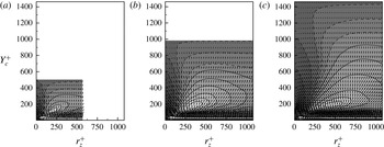
DNS of turbulent channel flows at (a)
 $\mathit{Re}_{{\it\tau}}=550$
, (b)
 $\mathit{Re}_{{\it\tau}}=1000$
and (c)
 $\mathit{Re}_{{\it\tau}}=1500$
. Energy source,
 ${\it\xi}^{+}(r_{x},r_{z},Y_{c})$
, isolines; and field of fluxes,
 $({\it\Phi}_{r_{z}}^{+},{\it\Phi}_{c}^{+})$
, vectors in the
 $r_{x}=0$
plane. Energy-source intensity increases from black to white. Solid lines denote positive values while dashed lines denote negative values.

4. The structure of the source term
The topological structure of the source term obtained from the three DNS datasets shows that all the basic characteristics observed at the lowest
 $\mathit{Re}_{{\it\tau}}$
are also maintained at higher Reynolds numbers. By analysing the data in the reduced space
 $(r_{x},r_{z},Y_{c})$
for
 $r_{y}=0$
, the source
 ${\it\xi}$
is found to reach its maximum at
 $r_{x}=0$
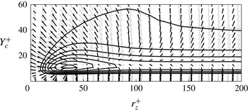
in a range of small spanwise scales well within the buffer layer; see figure 3. This region of the reduced space is a singularity point for the fluxes. As more clearly seen in figure 4, the scale-energy flux vector field has its origin in this peak of scale-energy source, which can be considered as the engine of wall turbulence and will be hereafter called the driving scale range (DSR). The small-scale location of the scale-energy source actually violates the classical paradigm of homogeneous isotropic turbulence. In wall flows, the turbulent energy is generated amid the spectrum of turbulent fluctuations, not at the largest scales, and this fact leads to a complex redistribution of energy (Cimarelli et al.
Reference Cimarelli, De Angelis and Casciola2013), with strong consequences for turbulence modelling (Cimarelli & De Angelis Reference Cimarelli and De Angelis2012; Cimarelli & De Angelis Reference Cimarelli and De Angelis2014).
Scaling of the near-wall scale-energy source (
 ${\it\xi}^{+}$
) and of the field of fluxes
 $({\it\Phi}_{r_{z}}^{+},{\it\Phi}_{c}^{+})$
in the
 $r_{x}=0$
plane. Grey isolines and vectors denote the
 $\mathit{Re}_{{\it\tau}}=1000$
case while black ones denote the
 $\mathit{Re}_{{\it\tau}}=1500$
case.

(a) Spanwise scale of maximum scale-energy source,
 $(\ell _{z}^{{\it\xi}_{max}})^{+}$
, as a function of the wall distance. Diamonds denote the
 $\mathit{Re}_{{\it\tau}}=1500$
case, circles the
 $\mathit{Re}_{{\it\tau}}=1000$
case and squares the
 $\mathit{Re}_{{\it\tau}}=550$
case. The dashed line denotes the quadratic increase near the wall,
 $(\ell _{z}^{{\it\xi}_{max}})^{+}=35+0.02Y_{c}^{+2}$
, while the solid lines denote the linear increase in the overlap layer,
 $(\ell _{z}^{{\it\xi}_{max}})/h=0.14+(Y_{c}/h)$
,
 $(\ell _{z}^{{\it\xi}_{max}})/h=0.14+1.16(Y_{c}/h)$
and
 $(\ell _{z}^{{\it\xi}_{max}})/h=0.14+1.4(Y_{c}/h)$
, expressed in viscous units, i.e.
 $(\ell _{z}^{{\it\xi}_{max}})^{+}=80+Y_{c}^{+}$
,
 $(\ell _{z}^{{\it\xi}_{max}})^{+}=145+1.16Y_{c}^{+}$
and
 $(\ell _{z}^{{\it\xi}_{max}})^{+}=215+1.4Y_{c}^{+}$
. (b) Energy source,
 ${\it\xi}^{+}$
, isolines in the
 $r_{x}=0$
plane for the
 $\mathit{Re}_{{\it\tau}}=1500$
case. The straight lines are
 $r_{z}^{+}={\it\gamma}({\it\xi}_{0}^{+})$
(
 $Y_{c}^{+}$
–
 ${\tilde{Y}}_{c}^{+}$
)
 $+\tilde{r}_{z}^{+}$
, where
 ${\it\xi}_{0}^{+}$
defines the iso-level of
 ${\it\xi}$
,
 ${\it\gamma}({\it\xi}_{0}^{+})\in [0.04,1.4]$
,
 $\tilde{r}_{z}^{+}=120$
and
 ${\tilde{Y}}_{c}^{+}=80$
.

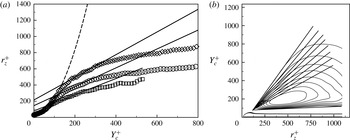
Another interesting feature emerging from the analysis of the Kolmogorov equation is the existence of a rescaled replica of the DSR, associated with a second peak in the scale-energy source, called hereafter outer driving scale range (ODSR). This outer peak of the scale-energy source has been observed in Cimarelli et al. (Reference Cimarelli, De Angelis and Casciola2013) and is present also at higher Reynolds numbers – see the isocontours of figure 3.
4.1. The driving scale range
In agreement with the picture of a universal near-wall region, the geometrical properties of the DSR are unaffected by the Reynolds number; see figure 4. For the three cases considered, the source peak within the DSR is located at
 $(r_{x}^{+},r_{z}^{+},Y_{c}^{+})=(0,40,12)$
. This Reynolds-number invariance and the clear matching of scales and positions suggests a strong connection with the near-wall cycle. Note that, for a given wall distance, the source maximum
 ${\it\xi}$
occurs at
 $r_{x}=0$
. Its location in the
 $(r_{z},Y_{c})$
plane, reported in figure 5(a), defines the typical spanwise scale of the scale-energy source,
 $(\ell _{z}^{{\it\xi}_{max}})^{+}$
. Near the wall, the spanwise location of the maximum increases quadratically with the wall distance,
 $(\ell _{z}^{{\it\xi}_{max}})^{+}\approx 35+0.02Y_{c}^{+2}$
, for all the Reynolds numbers considered. Clearly, within the DSR, for small distances from the wall,
 $Y_{c}^{+}<30$
, this trend results in an almost constant spanwise length scale: the typical spanwise scale of the most active structures of the wall is independent of the wall distance and Reynolds number. Although the topology of the DSR is basically
 $\mathit{Re}$
-invariant, its intensity is not. The scale-energy source is found to increase slightly with
 $\mathit{Re}_{{\it\tau}}$
. In particular, we measure
 ${\it\xi}_{max}^{+}=0.717$
, 0.732 and 0.741 on moving from lower to higher Reynolds number. This trend is consistent with the commonly observed mixed inner/outer scalings of the near-wall quantities. In fact, it is thought that the outer dynamics actively modulates the near-wall turbulence by producing small-scale fluctuations increasing Reynolds number (Marusic et al.
Reference Marusic, McKeon, Monkewitz, Nagib, Smits and Sreenivasan2010b
).
As shown by the vector field in figure 4, a direct consequence of the
 $\mathit{Re}$
invariance of the topology of the scale-energy source term,
 ${\it\xi}$
, is that also the scale-energy flux vector field,
 $({\it\Phi}_{r_{z}},{\it\Phi}_{c})$
, remains identical for increasing Reynolds number, once rescaled in viscous units. In this scenario, the Reynolds-number effects should come only from the ODSR in the overlap region. Indeed, even if the observed second peak of scale-energy source
 ${\it\xi}$
is very small compared to the one in the DSR, its relevance increases with
 $\mathit{Re}$
, as will be discussed in the next sections.
4.2. The outer driving scale range
The ODSR belongs to the overlap layer and appears to be the result of a second outer turbulent production mechanism well separated from the near-wall dynamics. The ODSR is separated from the DSR by a scale-energy sink region. Interestingly, this separation is found to be more pronounced with increasing
 $\mathit{Re}$
. The solid contour lines shown in figure 3 highlight that certain positive values for the source term
 ${\it\xi}$
are shared by both the DSR and ODSR for
 $\mathit{Re}_{{\it\tau}}=550$
. On the contrary, for larger Reynolds numbers, the DSR and ODSR are more and more separated by negative values for the source term
 ${\it\xi}$
, as shown by the number of dashed contour lines in between the inner and outer source shown in figure 3.
Although the peak intensity is smaller than the DSR one, the extent of the ODSR increases with
 $\mathit{Re}$
, suggesting how this object can play an important role at large Reynolds numbers. In contrast with the DSR, where production is concentrated at small scales that are independent of Reynolds number, the ODSR involves larger scales and its extent in inner units increases with
 $\mathit{Re}_{{\it\tau}}$
. For the three Reynolds numbers considered, the peak of the ODSR occurs in a well-defined scale region expressed in outer units corresponding to
 $r_{z}/h\approx 0.34$
. On the other hand, the physical location of the peak in the ODSR is
 $Y_{c}/h=(0.2;0.18;0.12)$
in outer units while
 $Y_{c}^{+}=(112;186;192)$
in viscous units going from low to high Reynolds number. Contrary to the space of scales,
 $r_{z}$
, which is found to be
 $\mathit{Re}$
-invariant once expressed in outer units, the wall distances,
 $Y_{c}$
, do not scale with
 $\mathit{Re}$
in neither inner nor outer units. This behaviour is probably related to the fact that the overlap layer extends from a lower limit given in viscous units to an upper limit in outer units, e.g. for
 $100<Y_{c}^{+}<0.2\mathit{Re}_{{\it\tau}}$
, but the exact values are still a matter of scientific debate; see Marusic et al. (Reference Marusic, McKeon, Monkewitz, Nagib, Smits and Sreenivasan2010b
) and references therein. These arguments suggest a mixed scaling with wall distance of the outer scale-energy source; see § 5 for a more detailed discussion. When considering the ODSR intensity, it is worth noting that the peak of scale-energy source in the ODSR remains essentially unaltered with Reynolds number once scaled in inner units and corresponds to
 ${\it\xi}^{+}\approx 0.0095$
.
The presence of the ODSR violates the equilibrium assumption of the overlap layer from which a local balance of production and dissipation is expected. Within the ODSR the energy injection is larger than the rate of dissipation,
 ${\it\xi}>0$
. As stated by (3.2), this fact results in a positive divergence of the energy transfer,
 $\boldsymbol{{\rm\nabla}}_{4}\boldsymbol{\cdot }{\it\bf\Phi}>0$
, which, under the assumption of a true equilibrium, is otherwise expected to be zero. This observation is consistent with the single-point energy excess already discussed in connection with figure 2 in § 2. Consequently, the overlap layer does not behave like a homogeneous shear flow traversed by a constant spatial flux of energy at both the single-point and two-point level. The ODSR continuously injects energy feeding the energy fluxes. As shown in figure 2, the spatial flux starts from the DSR in the buffer layer, it decreases by delivering energy in the sink layer wedged between the DSR and ODSR to increase again due to the energy injected by the ODSR leading to the second peak of the spatial flux. This second peak strongly depends on the Reynolds number, since the underlying physics of the ODSR belongs to the overlap layer whose extent, and, hence, its overall energy injection, increases with
 $\mathit{Re}$
, as figure 3 clearly suggests.
In this context, the existence of a simple near-wall viscous scaling may be questioned by the fact that different turbulent engines with different characteristic scales are at work, thus leading to anomalous scaling. It is generally thought that the mixed inner/outer scaling is due to the fact that, with increasing Reynolds number, the large-scale structures of the overlap layer become more energetic and able to actively modulate the near-wall dynamics through production of near-wall fluctuations (Hutchins & Marusic Reference Hutchins and Marusic2007b
; Mathis, Hutchins & Marusic Reference Mathis, Hutchins and Marusic2009; Marusic, Mathis & Hutchins Reference Marusic, Mathis and Hutchins2010a
; Marusic et al.
Reference Marusic, McKeon, Monkewitz, Nagib, Smits and Sreenivasan2010b
). Complementary to this picture, Jiménez (Reference Jiménez2012) describes this modulation as a local effect where small-scales structures equilibrate with their large-scale environment. From a point of view of scale-energy source and transfer, the mixed inner/outer scaling of the near-wall region could be interpreted as the result of a confinement of the scale-energy excess emerging from the near-wall region due to the presence of increasingly large production scales in the overlap layer. At given Reynolds number, the scale-energy flux originated in the DSR and directed towards the bulk of the flow encounters the additional energy source given by the ODSR. This additional energy source radiates scale energy and contributes to the overall energy flux. Below the ODSR the partial flux it generates is directed towards the wall, thereby opposing the flux produced in the DSR. The result is a net decrease in the flux towards the bulk. In fact, as stated by the turbulent kinetic energy and Kolmogorov equations (2.1) and (3.2), the source regions act to repulse the fluxes. Increasing the Reynolds number, the DSR remains fixed when scaled in inner units, while the effect of the ODSR increases. As shown in figure 3, the fluxes deviate to try to avoid the ODSR, which involves increasingly large scales with
 $\mathit{Re}$
. Hence, the overall effect is a decrease with Reynolds number of the scale-energy flux from the near-wall region due to the presence of increasingly large production scales with
 $\mathit{Re}$
in the ODSR. Accordingly, in the inset of figure 2(a) a decrease of the near-wall peak of the single-point spatial flux is observed at increasing
 $\mathit{Re}$
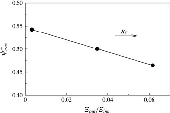
. This decrease is compared with the ratio between the overall outer and inner energy sources in figure 6. By increasing the Reynolds number, the ratio
 ${\it\Xi}_{out}/{\it\Xi}_{inn}$
increases and, as a consequence, the near-wall peak of the single-point spatial flux,
 ${\it\psi}_{max}^{+}$
, significantly decreases. In conclusion, the scale-energy produced within the DSR increasingly feeds the turbulence in the near-wall region since the energy flux towards the channel centre is decreasing with
 $\mathit{Re}$
. The resulting growth of the energy available near the wall is thus responsible for more intense fluctuations with
 $\mathit{Re}$
leading to a mixed inner/outer scaling of near-wall quantities.
Behaviour of the near-wall peak of the single-point spatial flux,
 ${\it\psi}_{max}^{+}$
, (2.1), as a function of the ratio
 ${\it\Xi}_{out}/{\it\Xi}_{inn}$
for increasing Reynolds number.

5. Overlap layer scalings
Let us now investigate in more detail the peculiar features of the Kolmogorov equation within the overlap layer. The first point we address is the behaviour with wall distance of the spanwise scale of maximum scale-energy source for a given wall distance,
 $\ell _{z}^{{\it\xi}_{max}}$
. The present data show that, for the three Reynolds numbers considered,
 $\ell _{z}^{{\it\xi}_{max}}$
increases almost linearly with
 $Y_{c}$
; see figure 5(a). In particular, we observe
 $\ell _{z}^{{\it\xi}_{max}}/h\sim 0.14+Y_{c}/h$
,
 $(\ell _{z}^{{\it\xi}_{max}})/h\approx 0.14+1.16(Y_{c}/h)$
and
 $(\ell _{z}^{{\it\xi}_{max}})/h\approx 0.14+1.4(Y_{c}/h)$
from low to high Reynolds numbers, respectively. This behaviour is similar to that reported in Saikrishnan et al. (Reference Saikrishnan, De Angelis, Longmire, Marusic, Casciola and Piva2012) for the shear scale
 $L_{s}$
, which is found to slightly increase its slope from
 $\mathit{Re}_{{\it\tau}}=300$
up to
 $\mathit{Re}_{{\it\tau}}=2000$
, where it seems to asymptotically approach the dimensional prediction
 $L_{s}=ky$
. In contrast to the slope, the intercept remains almost constant. This value of the intercept could be considered as the characteristic spanwise scale of the lower overlap layer. As shown by the isolines in figure 5(b) for
 $\mathit{Re}_{{\it\tau}}=1500$
, in the overlap layer the iso-levels of positive scale-energy source,
 ${\it\xi}>0$
, intercept spanwise scales that linearly increase with the distance from the wall. In particular, the iso-levels of
 ${\it\xi}$
can be approximated by a sheaf of lines originating from a unique point at
 $\tilde{r}_{z}^{+}=120$
and
 ${\tilde{Y}}_{c}^{+}=80$
but with different slopes, i.e.
 $r_{z}^{+}={\it\gamma}({\it\xi}_{0}^{+})(Y_{c}^{+}-{\tilde{Y}}_{c}^{+})+\tilde{r}_{z}^{+}$
, where
 ${\it\xi}_{0}^{+}$
defines the iso-level of
 ${\it\xi}$
and
 ${\it\gamma}({\it\xi}_{0}^{+})\in [0.04;1.4]$
.
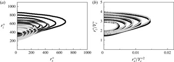
Scale-energy source isolines for three distances from the wall within the overlap layer for
 $\mathit{Re}_{{\it\tau}}=1500$
(
 $Y_{c}^{+}=140$
, light grey;
 $Y_{c}^{+}=180$
, dark grey; and
 $Y_{c}^{+}=220$
, black). (a) In inner units, the dimensions of the source region increase with the distance from the wall. (b) Spanwise and streamwise scales are normalized with the wall-normal distance and its square, respectively. Apparently, the isolines of the scale-energy source at different wall-normal distances tend to collapse one on top of the other.

As already stated, the source maximum is found at
 $r_{x}=0$
for all
 $Y_{c}$
, while for
 $r_{x}>0$
the source decreases; see figure 7(a). By tracking the spanwise scale of the maximum of
 ${\it\xi}$
as a function of the streamwise scale, we find that these spanwise scales increase following a square-root law,
 $r_{z}^{+}\sim \sqrt{r_{x}^{+}}$
, independently of the Reynolds number. This behaviour is similar to that reported by del Alamo et al. (Reference del Alamo, Jiménez, Zandonade and Moser2004) for the spectral distribution of the Reynolds stresses and it finds a possible theoretical explanation in Moarref et al. (Reference Moarref, Sharma, Tropp and McKeon2013) in terms of geometrically self-similar resolvent modes. Since we observe that the spanwise scales involved in the scale-energy source increase linearly with wall distance,
 $r_{z}^{+}\sim Y_{c}^{+}$
, we argue that the streamwise scales should behave quadratically with wall distance, i.e.
 $r_{x}^{+}\sim Y_{c}^{+2}$
. Hence, we expect the scale-space behaviour of the scale-energy source of the ODSR in the overlap layer to be approximately self-similar if plotted as a function of
 $r_{x}^{+}/Y_{c}^{+2}$
and
 $r_{z}^{+}/Y_{c}^{+}$
. As shown in figure 7(b) this rescaling of
 ${\it\xi}$
allows a unique comprehensive view of the outer scale-energy source where the
 $Y_{c}$
dependence is dropped. The data we have available at other Reynolds numbers (not shown) suggest that this behaviour is
 $\mathit{Re}_{{\it\tau}}$
independent. The comparison with figure 7(a) highlights that this single picture of the overall behaviour of the outer scale-energy source would be missed when using viscous units. It is worth mentioning that the observed scale-space distribution of the outer scale-energy source,
 $r_{z}^{+}\sim Y_{c}^{+}$
and
 $r_{x}^{+}\sim Y_{c}^{+2}$
, is consistent with the energy distribution found in Moarref et al. (Reference Moarref, Sharma, Tropp and McKeon2013), which, although different from the original scaling proposed by Townsend (Reference Townsend1976), is explained by the conjecture of an overlap layer populated by self-similar structures attached to the wall (see e.g. del Alamo et al.
Reference del Alamo, Jiménez, Zandonade and Moser2006).
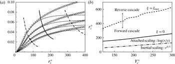
(a) Scaling of production,
 $-2\langle {\it\delta}u{\it\delta}v\rangle (\text{d}U/\text{d}y)$
, for
 $r_{x}=0$
and
 $\mathit{Re}_{{\it\tau}}=1500$
. From top to bottom the four solid lines provide the production at
 $Y_{c}^{+}=130$
,
 $160$
,
 $190$
and
 $230$
, respectively. Squares denote the logarithmic behaviour described by (5.2) and circles denote the inertial behaviour, (5.1). The three thick lines show the characteristic scales reported in panel (b). (b) The
 $Y_{c}$
behaviour of the scale of maximum scale-energy source,
 $(\ell _{z}^{{\it\xi}_{max}})^{+}\approx 215+1.4Y_{c}^{+}$
(dashed line), and of the zero scale-energy source,
 $(\ell _{z}^{{\it\xi}_{zero}})^{+}\approx 80+0.65Y_{c}^{+}$
(solid line). The shear scale,
 $\ell _{S}^{+}={\it\kappa}Y_{c}^{+}$
(dash-dotted line), represents the cross-over between logarithmic and power-law scaling of production.

We address now the possibility to scale also the intensity of the outer scale-energy source,
 ${\it\xi}=-2\langle {\it\delta}u{\it\delta}v\rangle (\text{d}U/\text{d}y)^{\ast }-4\langle {\it\epsilon}^{\ast }\rangle$
. The rate of viscous dissipation is constant in the space of scales and can be easily modelled by means of the equilibrium hypothesis,
 $\langle {\it\epsilon}\rangle \sim u_{{\it\tau}}^{3}/{\it\kappa}y$
. On the contrary, the scale-dependent behaviour of the production intensity is not trivial and needs a detailed analysis. Two distinct regimes are expected whose transition should be controlled by the shear scale
 $\ell _{S}$
(Jacob et al.
Reference Jacob, Casciola, Talamelli and Alfredsson2008). For scales larger than
 $\ell _{S}$
, the prevailing mechanism that determines the scaling law is production. For scales smaller than
 $\ell _{S}$
, the energy cascade prevails and an isotropy-recovering behaviour is expected to occur. This range should be characterized by a power law with universal exponents based on the dimensional predictions proposed by Lumley (Reference Lumley1965). As shown in figure 8(a) for
 $\mathit{Re}_{{\it\tau}}=1500$
(the same behaviour is observed also for the lower Reynolds numbers considered), the scale-energy production follows the classical Lumley’s prediction for the mixed structure function (Lumley Reference Lumley1965; Jacob et al.
Reference Jacob, Casciola, Talamelli and Alfredsson2008), here extended to scale-energy production by taking into account the mean shear,
 $\text{d}U/\text{d}y$
,
 $$\begin{eqnarray}-2\langle {\it\delta}u{\it\delta}v\rangle \frac{\text{d}U}{\text{d}y}=\frac{{\it\beta}u_{{\it\tau}}^{3}(r/y)^{4/3}}{{\it\kappa}y}\quad \text{for}~r<{\it\kappa}y,\end{eqnarray}$$
where
 ${\it\kappa}$
is the von Kármán constant; see circles in figure 8(a). Production follows this power law for scales smaller than the shear scale
 $\ell _{S}$
as shown by the thick dash-dotted line in figure 8(a). The shear scale defined as
 $\ell _{S}=\sqrt{{\it\epsilon}/S^{3}}$
, where
 $S=\text{d}U/\text{d}y$
, is computed here by using the overlap layer estimate,
 $\ell _{S}={\it\kappa}Y_{c}$
. Hence, the power law (5.1) is valid for scales smaller than the distance from the wall, the so-called detached scales. At scales larger than
 $\ell _{S}$
(attached scales), we find that the production in the overlap layer is well described by a logarithmic law,
 $$\begin{eqnarray}-2\langle {\it\delta}u{\it\delta}v\rangle \frac{\text{d}U}{\text{d}y}=\frac{u_{{\it\tau}}^{3}(C+D\log (r/y))}{{\it\kappa}y}\quad \text{for}~{\it\kappa}y<r<\ell _{z}^{{\it\xi}_{zero}};\end{eqnarray}$$
see squares in figure 8(a). This law is closely related to the (
 $k^{-1}$
) law for the energy spectrum derived by Perry, Hanbest & Chong (Reference Perry, Hanbest and Chong1986); see also Nikora (Reference Nikora1999). As shown in Davidson, Nickels & Krogstad (Reference Davidson, Nickels and Krogstad2006), the real-space analogue of the (
 $k^{-1}$
) law is a logarithmic law for the streamwise second-order structure functions. Equation (5.2) represents an extension of this law to the mixed structure functions,
 $\langle {\it\delta}u{\it\delta}v\rangle$
, which takes into account also the mean shear,
 $\text{d}U/\text{d}y$
. Scaling (5.2) remains valid up to
 $r_{z}=\ell _{z}^{{\it\xi}_{zero}}$
where
 $\ell _{z}^{{\it\xi}_{zero}}$
is defined as the scale where the source term becomes zero,
 ${\it\xi}=0$
. For scales smaller than
 $\ell _{z}^{{\it\xi}_{zero}}$
the source term is actually a sink for the scale-energy fluxes,
 ${\it\xi}<0$
, while for larger scales it is a source,
 ${\it\xi}>0$
.
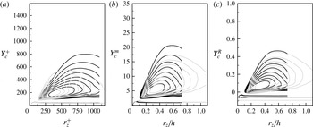
Energy source,
 ${\it\xi}^{+}$
, isolines in the
 $r_{x}=0$
plane for
 $\mathit{Re}_{{\it\tau}}=1000$
(grey) and
 $\mathit{Re}_{{\it\tau}}=1500$
(black):
 ${\it\xi}^{+}$
is shown as a function of (a) viscous quantity,
 $(r_{z}^{+},Y_{c}^{+})$
, (b) mixed quantity,
 $(r_{z}/h,Y_{c}^{m})$
, and (c) rescaled quantity,
 $(r_{z}/h,Y_{c}^{R})$
.

According to (3.2) and as shown by the vector field in figure 3, scales smaller than
 $\ell _{z}^{{\it\xi}_{zero}}$
are characterized by a negative divergence of the fluxes since
 ${\it\xi}<0$
and, thus, by a forward cascade. As a consequence, the logarithmic behaviour (5.2) is associated with turbulent scales involved in a forward cascade process. Since, as anticipated, these scales are larger than
 $\ell _{S}={\it\kappa}Y_{c}$
, they are influenced by the presence of the walls. On the other hand, the power-law scaling characterizes scales smaller than
 $\ell _{S}={\it\kappa}Y_{c}$
. Hence, the influence of the wall should be somehow negligible and, consequently, the forward cascade should resemble the classical one proposed by Kolmogorov since an isotropic recovery should start to take place (see Casciola et al.
Reference Casciola, Gualtieri, Jacob and Piva2005). It could be worth stressing that the shear scale, often identified with the distance from the wall, has long been addressed to explain the momentum and energy transfer between different scales of motion, starting from the pioneering work of Townsend (Reference Townsend1976) to more recent contributions (see e.g. Nikora Reference Nikora1999; Lozano-Duran & Jiménez Reference Lozano-Duran and Jiménez2014). As shown in figure 8(b), both
 $\ell _{S}$
and
 $\ell _{z}^{{\it\xi}_{zero}}$
linearly increase with the wall distance, denoting again statistical features attached to the wall. Since the slope of
 $\ell _{z}^{{\it\xi}_{zero}}$
is larger than that of the shear scale,
 $\ell _{S}$
, we can expect that the range of scales where the logarithmic scaling holds should expand significantly with Reynolds number, increasing the importance of the scaling for the prediction of production.
Figure 5 suggests a possible approximation for the source term for scales larger than
 $\ell _{z}^{{\it\xi}_{zero}}$
. By assuming that the production term for scales close to
 $\ell _{z}^{{\it\xi}_{max}}$
roughly behaves linearly with
 $r_{z}$
, see figure 8, we can model the source term as
 ${\it\xi}^{+}\approx A(Y_{c}^{+})r_{z}^{+}+B(Y_{c}^{+})$
since dissipation is a scale-independent process. In addition, we have also found in § 4.2 that the iso-levels of
 ${\it\xi}>0$
form a sheaf of lines described by the equation
 $r_{z}^{+}={\it\gamma}({\it\xi}_{0}^{+})(Y_{c}^{+}-{\tilde{Y}}_{c}^{+})+\tilde{r}_{z}^{+}$
, where
 ${\it\xi}_{0}^{+}$
defines the iso-level of
 ${\it\xi}$
we are considering (see figure 5). By combining these two pieces of information, the slope
 ${\it\gamma}$
is given by
 ${\it\gamma}({\it\xi}_{0}^{+})\approx G{\it\xi}_{0}^{+}+H$
, implying that the source term can be approximated as
 ${\it\xi}^{+}\approx (r_{z}^{+}-\tilde{r}_{z}^{+})/G(Y_{c}^{+}-{\tilde{Y}}_{c}^{+})-H/G$
. From our data we find
 $G=103.9$
and
 $H=0.58$
.
Summarizing, we have shown that for a fixed Reynolds number the complex multidimensional features of the ODSR can be described in a simple way by using the self-similarity of the streamwise and spanwise scales shown in figure 7 and the scaling of the production intensity shown in figure 8. Despite the limited range of Reynolds numbers we have available, let us address now how this picture changes for different Reynolds numbers. As already shown in § 4.2, the intensity of the outer scale-energy source scaled in viscous units and its scale-space location scaled in outer units remain constant for the present Reynolds numbers. Hence, the effect of Reynolds number mainly reduces to an expansion/shrinking of the wall-normal distances. A sufficiently general procedure could be to consider a mixed scaling of the wall-normal distance in the form
 $Y_{c}^{m}=(Y_{c}/h)^{{\it\alpha}}(Y_{c}^{+})^{{\it\beta}}$
. Alternatively one could use outer units shifting the origin according to the expression
 $Y_{c}^{R}=(Y_{c}/h)-{\it\eta}^{+}/\mathit{Re}_{{\it\tau}}$
, where
 ${\it\eta}^{+}$
is a free parameter. By considering
 ${\it\alpha}={\it\beta}=1/2$
in the first case and
 ${\it\eta}^{+}=100$
in the second one, the resulting scaling of the outer scale-energy source is shown in figure 9. Although not conclusive, given the small range of Reynolds numbers investigated, this result seems to be consistent with the possibility of a universal rescaling of the outer scale-energy source (ODSR).
6. Concluding remarks
By means of the description of turbulence given by the generalized Kolmogorov equation, we study the scale-energy transfer and production mechanisms of turbulent wall flows at different Reynolds numbers. Two driving mechanisms in terms of scale-energy source are identified for the fluxes. The first, stronger one, the driving scale range (DSR), belongs to the near-wall cycle. As expected, its inner-scaled topology remains unaltered with Reynolds number while its intensity is found to slightly increase with
 $\mathit{Re}$
(near-wall modulation). The second outer scale-energy source, the outer driving scale range (ODSR), takes place further away from the wall in the overlap layer and is separated from the DSR by a distinct scale-energy sink layer, suggesting a possible independence of the production mechanisms of the ODSR from the near-wall region, which might be interpreted as an autonomous outer cycle. Although its intensity is small compared to the DSR, the outer region of scale-energy source expands with Reynolds number while its peak intensity remains almost constant. These observations suggest the importance of the ODSR for large-Reynolds-number wall turbulence.
Further analysis of the ODSR demonstrates that the
 $\mathit{Re}$
dependence of the outer scale-energy source can be dropped by scaling in outer units the space of scales and in mixed units the wall distance, at least for the range of Reynolds numbers analysed here. Furthermore, we found that the spanwise scales involved in the scale-energy source linearly increase with the distance from the wall. On the other hand, the streamwise scales are connected to these spanwise scales of scale-energy source through a square-root law and, hence, quadratically increase with wall distance. These observations allow us to scale the outer scale-energy source, highlighting its self-similarities for different wall distances and Reynolds numbers. While considering the intensity of the outer scale-energy source, we found that the space of scales within the overlap layer can be divided into two distinct ranges. For scales larger than the shear scale,
 $\ell _{s}$
, but smaller than the cross-over scale of zero scale-energy source,
 $\ell _{z}^{{\it\xi}_{zero}}$
, the outer scale-energy source follows a logarithmic law,
 ${\it\xi}=u_{{\it\tau}}^{3}(C+D\log (r/y)-1)/{\it\kappa}y$
. This behaviour is theoretically consistent with the presence of a
 $k^{-1}$
law for the energy co-spectrum. For scales smaller than the shear scale, the outer scale-energy source follows a power law whose exponent equals Lumley’s dimensional prediction,
 ${\it\xi}=u_{{\it\tau}}^{3}({\it\beta}(r/y)^{4/3}-1)/{\it\kappa}y$
. These scales are involved in a direct cascade whose features should resemble the classical one since they are detached from the wall and, hence, an isotropic recovery is expected to take place. Interestingly, both
 $\ell _{z}^{{\it\xi}_{zero}}$
and
 $\ell _{s}$
increase linearly with wall distance. The different increase with wall distance of these two scales highlights the possible extension of the range of scales of validity of the logarithmic law for the prediction of outer scale-energy source at large Reynolds numbers. Overall, these observations suggest a strong connection of the observed outer scale-energy source with the presence of an outer turbulence production cycle whose statistical features agree with the hypothesis of an overlap layer dominated by self-similar structures attached to the wall.
The topology of the energy transfer is also studied. The paths of energy resemble the one reported in Cimarelli et al. (Reference Cimarelli, De Angelis and Casciola2013) for a lower-Reynolds-number case. Only one singularity point related to the DSR exists from which the fluxes depart also for larger Reynolds number. According to our observations we may expect a high-Reynolds-number state of wall turbulence where only one origin for the fluxes exists and corresponds to the DSR at the small scales of the near-wall region, since the intensity of the ODSR should be substantially
 $\mathit{Re}$
independent. In this scenario, the Reynolds-number effects on the energy transfer should come only from the expansion of the ODSR in both scale and physical space with
 $\mathit{Re}$
. For increasing Reynolds numbers, the turbulent energy emerging from the DSR near the wall experiences an expanding outer scale-energy source in the overlap layer, which acts to repulse the fluxes as stated by (3.2). Hence, the fluxes try to avoid the increasingly large production scales of the ODSR and remain partially confined to the wall region, increasing the overall amount of energy locally available near the wall. Accordingly, we observe a decrease of the spatial flux from the buffer to the overlap layer at increasing Reynolds numbers. Hence we may conjecture that the near-wall modulation is a result of a confinement of the near-wall source due to the presence of increasingly large production scales in the overlap layer.
Acknowledgements
We acknowledge PRACE for awarding us via the REFIT project access to resource Jugene at the Jülich Supercomputing Centre in Germany. Computational resources at PDC were made available by SNIC. G.B. acknowledges financial support by the Swedish Research Council (grant number 621-2013-5784).