1. Introduction
Vortex-induced vibration (VIV) is a popular research topic in the fields of fluid mechanics and fluid–structure interaction (FSI) because this phenomenon has a high application value in many fields of engineering, such as wind, ocean and aeronautical engineering. However, given that VIV contains rich and complex phenomena that have not been fully understood, the analysis of its mechanisms is significant in promoting fluid mechanics. Therefore, VIV is considered as a kaleidoscope in this research field. For a comprehensive review of the research on various aspects of VIV, one can refer to Sarpkaya (Reference Sarpkaya2004), Williamson & Govardhan (Reference Williamson and Govardhan2004) and Bearman (Reference Bearman2011).
In classical aeroelasticity, VIV is considered to be a dynamic response problem and is believed to be a type of forced vibration under the effect of unsteady vortex flow. This idea ignores the coupling effect between the fluid and the structure. Thus, the cylinder oscillation frequency
 $f$
should be completely determined by the vortex shedding frequency
 $f_{w}$
. However, researchers (e.g. Feng Reference Feng1968; Blevins Reference Blevins1990) have found that the vibration frequency of the cylinder no longer follows the vortex shedding frequency but becomes ‘locked-in’ to the natural frequency of the cylinder (
 $f_{s}$
) as the natural frequency of the cylinder approaches the vortex shedding frequency of the fixed cylinder. Simultaneously, a large vibration amplitude of the cylinder is observed within the lock-in regime. This abnormal phenomenon is often referred to as ‘frequency lock-in’ or ‘synchronization’ in VIV.
A substantial number of studies have focused on understanding the frequency lock-in phenomenon by applying either experimental or numerical methods. The effects of the mass ratio (Prasanth, Premchandran & Mittal Reference Prasanth, Premchandran and Mittal2011), the structural damping coefficient (Nguyen et al.
Reference Nguyen, Koide, Yamada, Takahashi and Shirakashi2012) and the Reynolds number (Govardhan & Williamson Reference Govardhan and Williamson2006) on the lock-in regime have also been extensively studied. However, the study on the induced mechanisms of frequency lock-in has not been thorough. Most researchers have attributed the frequency lock-in phenomenon in VIV to resonance or the nonlinear feedback effect of FSIs. Since the work of Den Hartog (Reference Den Hartog1934), the conventional view has been that large-amplitude oscillations occurring at velocities where the vortex shedding frequency is comparable with the natural frequency are caused by resonance. Govardhan & Williamson (Reference Govardhan and Williamson2000, Reference Govardhan and Williamson2002) further demonstrated that when the value of the mass is below a critical value, the regime of reduced velocity
 $U^{\ast }$
for resonant oscillations can be infinitely wide, beginning at approximately
 $U^{\ast }\sim 5$
and extending to
 $U^{\ast }\sim \infty$
. Furthermore, Willden & Graham (Reference Willden and Graham2006) found that at low Reynolds numbers (
 $Re\leqslant 400$
), transversely vibrating circular cylinders may exhibit three distinct regions of response, and the primary response region occurs at or around resonance. They also pointed out that never-ending resonance or infinite lock-in may occur at sufficiently low mass ratios.
However, the most commonly accepted interpretation that frequency lock-in is caused by simple resonance has its limitations. For example, Singh & Mittal (Reference Singh and Mittal2005) conducted numerical simulations to investigate VIV by using a finite element method. In one of their cases, they fixed
 $Re$
at 100 and varied the reduced velocity (
 $U^{\ast }$
). Their results show that the maximum vibration amplitude of the cylinder is acquired at a relatively high frequency ratio of
 $f_{s}/f_{w}\sim 1.28$
rather than at the synchronized point where
 $f_{s}/f_{w}\sim 1.0$
. This anomaly is difficult to explain from the perspective of resonance. Moreover, the amplitude of the lift coefficient varies significantly in the lock-in regime (the amplitude of the lift coefficient is 1.1 for
 $f_{s}/f_{w}\sim 1.28$
and approximately 0.02 for
 $f_{s}/f_{w}\sim 0.90$
). Similar conclusions can be obtained from the numerical results of Zhou, So & Lam (Reference Zhou, So and Lam1999). However, the authors did not conduct any further analysis or discussion of this phenomenon. This shortcoming leads to the question of what underlying physical mechanism induces frequency lock-in and the occurrence of large vibration amplitude at high natural frequencies.
Theoretical modelling methods, in either a semi-analytical or semi-empirical manner, have been widely utilized to study the dynamics of VIV at high Reynolds numbers. These types of models can be classified into two groups, namely the wake oscillator model and the force decomposition model. Hartlen & Currie (Reference Hartlen and Currie1970) formulated the most noteworthy of the wake oscillator models. In such models, a van der Pol oscillator is employed to represent the wake dynamics. Facchinetti, De Langre & Biolley (Reference Facchinetti, De Langre and Biolley2002, Reference Facchinetti, De Langre and Biolley2004a ,Reference Facchinetti, De Langre and Biolley b ) have shown that a few main features of the VIV phenomenology can be retrieved by using this type of nonlinear coupled model. In particular, the range of lock-in and its dependence on the mass ratio can be well described. De Langre (Reference De Langre2006) utilized a linearized wake oscillator model of the simplest form; all nonlinear and dissipative terms were neglected in his research. The resulting linear system was constructed by coupling the wake oscillator model and the structural oscillator. The stability analysis results showed that frequency lock-in is primarily caused by coupled-mode flutter. The extent of the lock-in range was successfully predicted. This analytical idea opened a new threshold for the interpretation of the frequency lock-in phenomenon. Besides, linear wake oscillator models have also been utilized to study VIV of slender flexible structures like cables and strings (Violette, De Langre & Szydlowski Reference Violette, De Langre and Szydlowski2010; Grouthier et al. Reference Grouthier, Michelin, Modarres-Sadeghi and De2013). The stability analysis results showed that linear models could capture a significant part of the underlying physics of the VIV phenomenon.
The force decomposition method was first proposed by Sarpkaya (Reference Sarpkaya1978), who divided the force acting on an elastically suspended cylinder into fluid inertia and the fluid damping force. Chen, Zhu & Cai (Reference Chen, Zhu and Cai1995) developed an unsteady theory for VIV. They represented the force arising from the FSI by three linear motion-dependent components and concluded that VIV is composed of instability and forced vibration. Zhu et al. (Reference Zhu, Wang, Xie and So2008) showed that the flow-induced vibration of a circular cylinder in the lock-in region is a combination of forced vibration and fluid-damping-induced instability, which may lead to time-dependent fluid-damping-induced parametric resonance and constant-negative damping-induced instability. However, the abovementioned theoretical models rely heavily on experimental results and often do not include any analysis of the flow field; their best value is in explaining and simulating experimental results (Dowell Reference Dowell1980; Gabbai & Benaroya Reference Gabbai and Benaroya2005). Therefore, these explanations for the lock-in mechanisms by theoretical models have not elicited much attention so far.
Given the complexity of FSI problems and the lack of ideal theoretical models, direct experimental and numerical methods have difficulty in addressing the underlying physical mechanisms of frequency lock-in in VIV. Therefore, in recent years, many researchers have resorted to dynamics stability analysis methods, such as the global linear stability analysis (LSA) method, to investigate VIV phenomenology. A limited number of studies have concentrated on the instability of VIV near the critical Reynolds number (
 $Re_{cr}\sim 47$
). Cossu & Morino (Reference Cossu and Morino2000) conducted a global stability analysis of an elastically supported cylinder at subcritical
 $Re$
based on linearized Navier–Stokes equations. They found that the critical Reynolds number
 $Re_{cr}$
for a cylinder with fluid-to-solid density ratio larger than
 $1/70$
is less than half that of the stationary structure case. This phenomenon was further confirmed by Buffoni (Reference Buffoni2003) through experiments and Mittal & Singh (Reference Mittal and Singh2005) through direct numerical simulations. Two significant modes for the vibrating cylinder were identified in their study, namely a ‘nearly structural’ mode and a von Karman mode. These two modes correspond to eigenvalues that, in the limit of very high mass ratios (i.e. very weak FSI), tend to approach the natural frequency of the cylinder in the absence of fluid and the leading eigenvalues of the ‘purely fluid’ system with a fixed cylinder. These authors have proven that the occurrence of vortex shedding at subcritical Reynolds numbers is due to the instability of the structure mode. Furthermore, Meliga & Chomaz (Reference Meliga and Chomaz2011) investigated the instability characteristics of the coupled system through an asymptotic expansion method. They showed that the mass ratio plays an important role in the selection of the leading mode. They also extended this method to the nonlinear analysis of VIV.
Apart from the global LSA method (Cai, Liu & Luo Reference Cai, Liu and Luo2003; Crouch, Garbaruk & Magidov Reference Crouch, Garbaruk and Magidov2007; Crouch et al.
Reference Crouch, Garbaruk, Magidov and Travin2009; Leontini, Thompson & Hourigan Reference Leontini, Thompson and Hourigan2010), the system identification method (Zhang & Ye Reference Zhang and Ye2007; Dahan, Morgans & Lardeau Reference Dahan, Morgans and Lardeau2012; Illingworth, Morgans & Rowley Reference Illingworth, Morgans and Rowley2012; Brunton, Rowley & Williams Reference Brunton, Rowley and Williams2013) has also been utilized for the characteristic analysis of unsteady flows in recent years. The present study focuses on finding a more accurate aerodynamic model for the cylinder wake flow by using a system identification method. A reduced-order model (ROM) is coupled with structural motion equations to form an ROM-based FSI model. Eigenvalue analysis of the ROM-based FSI model is then performed, and the effects of the mass ratio and the structural damping coefficient on the dynamics of VIV are studied for
 $Re=60$
. The frequency lock-in phenomenon in VIV is interpreted through linear dynamics. Direct computational fluid dynamics/computational structural dynamics (CFD/CSD) simulations are simultaneously conducted to validate the results analysed by the ROM-based FSI model.
2. The CFD method and its validation
2.1. Navier–Stokes equations and finite-volume formulation
Accurate calculation of unsteady aerodynamic loads is the basis of investigating VIVs. In this study, the full compressible Navier–Stokes equations are utilized to simulate the essentially two-dimensional incompressible laminar flow past a circular cylinder at low Reynolds numbers. The Mach number is very small, and is taken to be
 $\mathit{Ma}=0.1$
. The integral conservation governing equations, with all geometrical length scales normalized with the cylinder diameter (
 $D$
), streamwise and cross-stream velocities with the free-stream flow speed (
 $U_{\infty }$
), physical time with (
 $D/U_{\infty }$
) and pressure with (
 ${\it\rho}U_{\infty }^{2}$
), are given as follows:
 $$\begin{eqnarray}\frac{\partial }{\partial t}\iint _{{\it\Omega}}\boldsymbol{Q}\,\text{d}V+\oint _{\partial {\it\Omega}}\boldsymbol{F}(\boldsymbol{Q},\boldsymbol{V}_{grid})\boldsymbol{\cdot }\boldsymbol{n}\,\text{d}S=\oint _{\partial {\it\Omega}}\boldsymbol{G}(\boldsymbol{Q})\boldsymbol{\cdot }\boldsymbol{n}\,\text{d}S,\end{eqnarray}$$
where
 ${\it\Omega}$
denotes the control surface element,
 $\partial {\it\Omega}$
represents the boundary of the control surface element and
 $\boldsymbol{n}$
is the identity normal vector. The vector of conservative variables
 $\boldsymbol{Q}$
, the inviscid flux vector
 $\boldsymbol{F}(\boldsymbol{Q},\boldsymbol{V}_{grid})$
considering the grid moving velocity
 $\boldsymbol{V}_{grid}$
, and the viscous flux vector
 $\boldsymbol{G}(\boldsymbol{Q})$
are given by the following equations:
 $$\begin{eqnarray}\displaystyle \left.\begin{array}{@{}c@{}}\displaystyle \boldsymbol{Q}=\left[\begin{array}{@{}c@{}}{\it\rho}\\ {\it\rho}u\\ {\it\rho}v\\ e_{0}\\ \end{array}\right],\quad \boldsymbol{F}_{x}(\boldsymbol{Q},\boldsymbol{V}_{grid})=\left[\begin{array}{@{}c@{}}{\it\rho}(u-u_{grid})\\ {\it\rho}u(u-u_{grid})+P\\ {\it\rho}(u-u_{grid})v\\ e_{0}(u-u_{grid})+Pu\\ \end{array}\right],\\ \boldsymbol{F}_{y}(\boldsymbol{Q},\boldsymbol{V}_{grid})=\left[\begin{array}{@{}c@{}}\displaystyle {\it\rho}(v-v_{grid})\\ \displaystyle {\it\rho}u(v-v_{grid})\\ \displaystyle {\it\rho}(v-v_{grid})v+P\\ \displaystyle e_{0}(v-v_{grid})+Pv\\ \end{array}\right],\\ \displaystyle \boldsymbol{G}_{x}(\boldsymbol{Q})={\it\mu}\left[\begin{array}{@{}c@{}}0\\ \displaystyle 2u_{x}-\frac{2}{3}(u_{x}+v_{y})\\ v_{x}+u_{y}\\ \displaystyle u\left[2u_{x}-\frac{2}{3}(u_{x}+v_{y})\right]+v(v_{x}+u_{y})+\frac{1}{{\it\gamma}-1}\frac{T_{x}}{Pr}\\ \end{array}\right],\\ \boldsymbol{G}_{y}(\boldsymbol{Q})={\it\mu}\left[\begin{array}{@{}c@{}}0\\ v_{x}+u_{y}\\ \displaystyle 2v_{y}-\frac{2}{3}(u_{x}+v_{y})\\ \displaystyle u(v_{x}+u_{y})+v\left[2v_{y}-\frac{2}{3}(u_{x}+v_{y})\right]+\frac{1}{{\it\gamma}-1}\frac{T_{y}}{Pr}\\ \end{array}\right],\end{array}\right\} & & \displaystyle\end{eqnarray}$$
where
 ${\it\rho}$
is the density,
 $u,v$
are
 $x$
-wise and
 $y$
-wise components of the velocity vector of the flow,
 $u_{grid},v_{grid}$
are
 $x$
-wise and
 $y$
-wise components of the velocity vector of the grid movement, and
 $e_{0},P$
denote the total energy and pressure respectively. The subscripts
 $x$
and
 $y$
denote the partial derivatives of the flow velocity,
 $T$
is the temperature,
 $Pr$
is the Prandtl number and
 ${\it\gamma}=1.4$
is the ratio of specific heats. Here,
 ${\it\mu}$
denotes the dynamic molecular viscosity, which is computed by Sutherland’s law:
 $$\begin{eqnarray}{\it\mu}=\frac{1.45T^{3/2}}{T+110}\times 10^{-6}.\end{eqnarray}$$
When the cell-centred finite-volume method is applied for each grid, the spatial discretization of (2.1) can be expressed as
 $$\begin{eqnarray}\frac{\text{d}\,(\boldsymbol{Q}_{i})}{\text{d}t}=-\frac{1}{{\it\Omega}_{i}}\mathop{\sum }_{m\in N(i)}[\boldsymbol{F}(\boldsymbol{Q},\boldsymbol{V}_{grid})_{im}-\boldsymbol{G}(\boldsymbol{Q})_{im}]\boldsymbol{S}_{im},\end{eqnarray}$$
where
 ${\it\Omega}_{i}$
represents the volume of grid cell
 $i$
,
 $N(i)$
is the sum of cell faces,
 $\boldsymbol{S}_{im}$
is the normal vector area of the face and the subscript
 $im$
denotes the current face that is shared by cells
 $i$
and
 $m$
. The AUSM
 $+$
-up scheme is utilized for the calculation of the inviscid flux vector
 $\boldsymbol{F}(\boldsymbol{Q},\boldsymbol{V}_{grid})_{im}$
. The discretization of the viscous flux term
 $\boldsymbol{G}(\boldsymbol{Q})_{im}$
is usually conducted using the standard central scheme because of the elliptic nature of this term.
For the semi-discrete equation (2.4), we adopt the implicit discretization for flux terms, and the three-point backward-difference approximation of the time derivative is shown as
 $$\begin{eqnarray}\frac{3\boldsymbol{Q}_{i}^{n+1}-4\boldsymbol{Q}_{i}^{n}+\boldsymbol{Q}_{i}^{n-1}}{2{\rm\Delta}t}+\boldsymbol{R}_{i}(\boldsymbol{Q}_{i}^{n+1})=0,\end{eqnarray}$$
where
 $$\begin{eqnarray}\boldsymbol{R}_{i}(\boldsymbol{Q}_{i}^{n+1})=\frac{1}{{\it\Omega}_{\,i}}\mathop{\sum }_{m\in N(i)}[\boldsymbol{F}(\boldsymbol{Q},\boldsymbol{V}_{grid})_{im}-\boldsymbol{G}(\boldsymbol{Q})_{im}]\boldsymbol{S}_{im}.\end{eqnarray}$$
The symbol
 ${\rm\Delta}t$
denotes the real time step and the superscript
 $n+1$
represents the value of the new time level. Equation (2.5) is solved by the implicit dual time-stepping scheme. The main idea of the dual time-stepping approach is to add the pseudo-time level to the left of the governing equations. Thus, we obtain the following:
 $$\begin{eqnarray}\frac{\text{d}\boldsymbol{Q}_{i}^{n+1}}{\text{d}{\it\tau}}+\frac{3\boldsymbol{Q}_{i}^{n+1}-4\boldsymbol{Q}_{i}^{n}+\boldsymbol{Q}_{i}^{n-1}}{2{\rm\Delta}t}+\boldsymbol{R}_{i}(\boldsymbol{Q}_{i}^{n+1})=0,\end{eqnarray}$$
where
 ${\it\tau}$
denotes the pseudo-time variable. The implicit symmetric Gauss–Seidel iterative time-marching scheme is employed for the solution of (2.7) on the pseudo-time level. When the scheme is fulfilled, i.e.
 $\text{d}\boldsymbol{Q}_{i}^{n+1}/\text{d}{\it\tau}=0$
, we obtain a steady state in pseudo-time. The real solution of the new time level
 $\boldsymbol{Q}_{i}^{n+1}$
is also obtained. For more details, one can refer to the PhD thesis of Jiang (Reference Jiang2013).
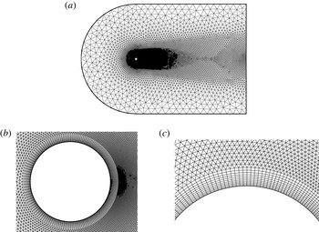
(a) Hybrid grid and (b,c) close-up views of the hybrid grid.

2.2. Boundary conditions and grid deformation scheme
A no-slip wall boundary condition is applied to the cylinder surface. The location and velocity of the cylinder are updated at each real time step due to the motion of cylinder. Moreover, the far-field boundary is assigned a non-reflective boundary condition to ensure that the disturbance generated by the object is not returned within the flow field. Widely utilized Riemann invariants are adopted to deal with the far-field non-reflective boundary conditions.
Figure 1 shows domain discretization with a close-up view of the hybrid grid used in this study near the inner boundary. The unstructured hybrid mesh used for most of the computations in this paper consists of 21 414 nodes and 40 324 cells. We refer to this mesh as M21k. The overall size of the domain is
 $60D$
in the streamwise direction and
 $40D$
along the cross-streamwise direction. The centre of the cylinder is
 $20D$
from the upstream boundary.
A moving boundary is involved in the simulation due to the cylinder motion. Thus, a grid deformation method must be used to match the grid with the new wall boundary condition. In this paper, grid deformation is realized by using the radial base function interpolation scheme. More details on the grid moving scheme can be found in De Boer, Van der Schoot & Bijl (Reference De Boer, Van der Schoot and Bijl2007).
2.3. Validation of the CFD method
2.3.1. Laminar flow past a fixed cylinder
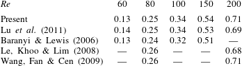
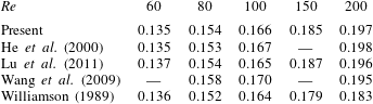
Computations were conducted for flow past a stationary circular cylinder at several typical Reynolds numbers (60, 80, 100, 150, and 200). The numerical validations focused on the amplitude of the lift coefficient
 $C_{L}^{max}$
and the Strouhal number
 $St$
. The compared results are shown in tables 1 and 2. Most of the present results are in good agreement with those of previous studies. Thus, the present numerical method is reliable. It is worth nothing that the Strouhal number for
 $Re=200$
measured from experiment (Williamson Reference Williamson1989) is very different from those calculated by numerical methods. The difference is mainly due to the three-dimensional character of the flow for this Reynolds number.
Comparison of the amplitude of the lift coefficient (
 $C_{L}^{max}$
) at different Reynolds numbers.

Comparison of the Strouhal number (
 $St$
) at different Reynolds numbers.

2.3.2. Laminar flow past a transversely oscillating cylinder
Given that the linear ROMs were constructed by perturbing the flow through cylinder motion, further validation of the present numerical method under forced vibrations is necessary. Mittal & Singh (Reference Mittal and Singh2005) investigated the relationship between the frequency of oscillation and the amplitude of the lift coefficient at
 $Re=33$
. To address this issue, they conducted computations for an oscillating cylinder at a fixed amplitude of
 $0.25D$
with varying vibrating frequencies.
We performed a calculation in which the cylinder was forced to vibrate in the form
 $h=0.25D\sin (2{\rm\pi}/U^{\ast }t)$
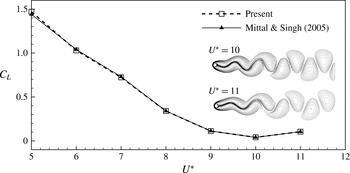
, and the calculated results are shown in figure 2. The results are in fairly good agreement with those of Mittal & Singh (Reference Mittal and Singh2005). A significant variation was observed in the amplitude of the lift coefficient with
 $U^{\ast }$
. The calculated results indicate that the amplitude of the lift coefficient depends heavily on the frequency of oscillations.
Flow past a forced vibrating cylinder: amplitude of the lift coefficient and vorticity fields for two typical values of
 $U^{\ast }$
at
 $Re=33$
.

3. Unsteady aerodynamic loads modelling for FSI
3.1. Reduced-order modelling method
An identification technique was employed to construct the reduced-order unsteady aerodynamic model at a typical Reynolds number. The model was trained by perturbing the flow with the cylinder motion using the direct numerical method proposed in § 2. Given that the unsteady loads were calculated in the discrete domain, the autoregressive with exogenous input (ARX) model can be utilized for the input–output system, which is expressed as follows:
 $$\begin{eqnarray}\boldsymbol{y}_{\boldsymbol{F}}(k)=\mathop{\sum }_{i=1}^{na}\unicode[STIX]{x1D63C}_{\boldsymbol{i}}\boldsymbol{y}_{\boldsymbol{F}}(k-i)+\mathop{\sum }_{i=1}^{nb}\unicode[STIX]{x1D63D}_{\boldsymbol{i}}\boldsymbol{u}(k-i),\end{eqnarray}$$
where
 $\boldsymbol{y}_{\boldsymbol{F}}$
is the output vector of the system and
 $\boldsymbol{u}$
is the input vector of the system. Here,
 $\unicode[STIX]{x1D63C}_{\boldsymbol{i}}$
and
 $\unicode[STIX]{x1D63D}_{\boldsymbol{i}}$
are the constant coefficients to be estimated, and
 $na$
and
 $nb$
are the delay orders determined by the user. For the current single-input–single-output model,
 $\boldsymbol{u}=[h]$
(transverse displacement of the cylinder) and
 $\boldsymbol{y}_{\boldsymbol{F}}=[C_{L}]$
(lift coefficient).
To derive the state-space form for aeroelastic analysis, we defined a state vector
 $\boldsymbol{x}_{\boldsymbol{F}}(k)$
consisting of (
 $na+nb-1$
) vector states as follows:
 $$\begin{eqnarray}\boldsymbol{x}_{\boldsymbol{F}}(k)=[y_{F}(k-1),\ldots ,y_{F}(k-na),u(k-1),\ldots ,u(k-nb+1)]^{\text{T}}.\end{eqnarray}$$
The state-space form for the discrete-time aerodynamic model can be described as follows:
 $$\begin{eqnarray}\left.\begin{array}{@{}c@{}}\boldsymbol{x}_{\boldsymbol{F}}(k+1)=\tilde{\unicode[STIX]{x1D63C}}_{\boldsymbol{F}}\boldsymbol{x}_{\boldsymbol{F}}(k)+\tilde{\unicode[STIX]{x1D63D}}_{\boldsymbol{F}}u(k),\\ y_{F}(k)=\tilde{\unicode[STIX]{x1D63E}}_{\boldsymbol{F}}\boldsymbol{x}_{\boldsymbol{F}}(k)+\tilde{\unicode[STIX]{x1D63F}}_{\boldsymbol{F}}u(k),\end{array}\right\}\end{eqnarray}$$
where
 $$\begin{eqnarray}\left.\begin{array}{@{}c@{}}\tilde{\unicode[STIX]{x1D63C}}_{\boldsymbol{F}}=\left[\begin{array}{@{}cccccccccc@{}}\unicode[STIX]{x1D63C}_{1} & \unicode[STIX]{x1D63C}_{2} & \cdots \, & \unicode[STIX]{x1D63C}_{na-1} & \unicode[STIX]{x1D63C}_{na} & \unicode[STIX]{x1D63D}_{1} & \unicode[STIX]{x1D63D}_{2} & \cdots \, & \unicode[STIX]{x1D63D}_{nb-2} & \unicode[STIX]{x1D63D}_{nb-1}\\ \unicode[STIX]{x1D644} & \mathbf{0} & \cdots \, & \mathbf{0} & \mathbf{0} & \mathbf{0} & \mathbf{0} & \cdots \, & \mathbf{0} & \mathbf{0}\\ \vdots & \unicode[STIX]{x1D644} & \cdots \, & \boldsymbol{ 0} & \boldsymbol{ 0} & \mathbf{0} & \mathbf{0} & \cdots \, & \boldsymbol{ 0} & \boldsymbol{ 0}\\ \vdots & \vdots & \ddots & \vdots & \vdots & \vdots & \vdots & \ddots & \vdots & \vdots \\ \mathbf{0} & \mathbf{0} & \cdots \, & \unicode[STIX]{x1D644} & \boldsymbol{ 0} & \mathbf{0} & \mathbf{0} & \cdots \, & \boldsymbol{ 0} & \boldsymbol{ 0}\\ \mathbf{0} & \mathbf{0} & \cdots \, & \mathbf{0} & \mathbf{0} & \mathbf{0} & \mathbf{0} & \cdots \, & \mathbf{0} & \mathbf{0}\\ \mathbf{0} & \mathbf{0} & \cdots \, & \boldsymbol{ 0} & \boldsymbol{ 0} & \unicode[STIX]{x1D644} & \mathbf{0} & \cdots \, & \boldsymbol{ 0} & \boldsymbol{ 0}\\ \mathbf{0} & \mathbf{0} & \cdots \, & \mathbf{0} & \mathbf{0} & \mathbf{0} & \unicode[STIX]{x1D644} & \cdots \, & \mathbf{0} & \mathbf{0}\\ \vdots & \vdots & \ddots & \vdots & \vdots & \vdots & \vdots & \ddots & \vdots & \vdots \\ \mathbf{0} & \mathbf{0} & \cdots \, & \mathbf{0} & \mathbf{0} & \mathbf{0} & \mathbf{0} & \cdots \, & \unicode[STIX]{x1D644} & \mathbf{0}\end{array}\right],\\ \tilde{\unicode[STIX]{x1D63D}}_{\boldsymbol{F}}=\left[\begin{array}{@{}cccccccccc@{}}\tilde{\unicode[STIX]{x1D63D}}_{0} & \mathbf{0} & \mathbf{0} & \cdots \, & \mathbf{0} & \unicode[STIX]{x1D644} & \mathbf{0} & \mathbf{0} & \cdots \, & \mathbf{0}\end{array}\right]^{\text{T}},\\ \tilde{\unicode[STIX]{x1D63E}}_{\boldsymbol{F}}=\left[\begin{array}{@{}cccccccccc@{}}\unicode[STIX]{x1D63C}_{1} & \unicode[STIX]{x1D63C}_{2} & \cdots \, & \unicode[STIX]{x1D63C}_{na-1} & \unicode[STIX]{x1D63C}_{na} & \unicode[STIX]{x1D63D}_{1} & \unicode[STIX]{x1D63D}_{2} & \cdots \, & \unicode[STIX]{x1D63D}_{nb-2} & \unicode[STIX]{x1D63D}_{nb-1}\end{array}\right],\\ \tilde{\unicode[STIX]{x1D63F}}_{\boldsymbol{F}}=\left[\unicode[STIX]{x1D63D}_{\mathbf{0}}\right].\end{array}\right\}\end{eqnarray}$$
To couple the structural equations, the discrete-time state-space form was converted into the continuous-time form. The model for the continuous-time state-space form was constructed as follows:
 $$\begin{eqnarray}\left.\begin{array}{@{}c@{}}\dot{\boldsymbol{x}}_{\boldsymbol{F}}(t)=\unicode[STIX]{x1D63C}_{\boldsymbol{F}}\boldsymbol{x}_{\boldsymbol{F}}(t)+\unicode[STIX]{x1D63D}_{\boldsymbol{F}}u(t),\\ y_{F}(t)=\unicode[STIX]{x1D63E}_{\boldsymbol{F}}\boldsymbol{x}_{\boldsymbol{F}}(t)+\unicode[STIX]{x1D63F}_{\boldsymbol{F}}u(t).\end{array}\right\}\end{eqnarray}$$
As we constructed the state-space model of the unsteady aerodynamic loads, the instability problems of the flow were converted into solving and analysing the eigenvalues of the matrix
 $\unicode[STIX]{x1D63C}_{\boldsymbol{F}}$
of the state-space equations. A more detailed process can be found in Zhang & Ye (Reference Zhang and Ye2007).
3.2. Validation of the reduced-order modelling method
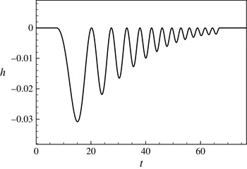
Signal design is the key element in dynamics modelling. The frequency coverage of the training signals should include the frequencies of the modes that need to be excited. The training amplitude should not be too large; otherwise, the aerodynamic responses would be nonlinear and the linear ARX modelling method cannot be employed. In this study, a chirp signal with a broadband reduced frequency [0.04, 0.20] was used as the training signal (figure 3). The numerical results show that the non-dimensional vortex shedding frequency for
 $Re=60$
is approximately 0.135. Thus, the designed signal is appropriate.
We know that it is difficult to identify a linear aerodynamics model based on the full developed unsteady vortex flow. Therefore, in the present paper, the ROMs are trained by performing the given signal on the steady-state base flows. The steady-state solutions of unsteady flows can be computed exactly by dropping the unsteady terms from the governing equations (Mittal Reference Mittal2008). We consider the aerodynamic modelling of
 $Re=45$
and
 $Re=60$
as examples to verify the correctness of the reduced-order method proposed in § 3.1. In order to accurately predict the unsteady aerodynamic loads, the delay orders are taken to be relatively large numbers here, i.e.
 $na=nb=100$
.
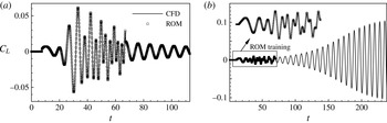
The identified results are compared with those of direct numerical simulations in figure 4; good agreement is observed between the two results. Therefore, we conclude that the identification method based on the ARX model has high numerical accuracy.
The training signal.

The ROMs are then validated in the time domain by comparing their harmonic forcing responses with those of direct numerical results. The harmonic forcing signal is in the form of
 $h=A\sin (2{\rm\pi}Ft)$
, where
 $A$
is the vibration amplitude of the cylinder and
 $F$
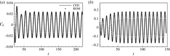
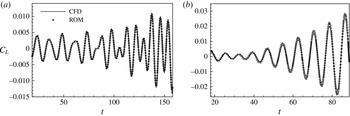
is the reduced frequency of forced vibration. Figures 5 and 6 show comparisons of the time histories of the lift coefficient predicted by ROMs and CFD simulations at two typical reduced frequencies (i.e.,
 $2{\rm\pi}F=0.5$
and
 $2{\rm\pi}F=0.8$
). In the case of subcritical Reynolds number
 $Re=45$
, the ROM predictions exactly match those computed by the direct numerical simulations. In the case of supercritical Reynolds number
 $Re=60$
, the ROM also provides surprisingly good predictions for the initial development stage of the original system. However, as time goes on, the aerodynamic system will gradually be dominated by vortex shedding, which is due to nonlinear dynamics. As expected, after a long period of time, the growing amplitude of the lift coefficient eventually gives rise to nonlinear dynamics and the solutions diverge to nonlinear limit-cycling states that are not captured by linear dynamics models.
Identified results under the training signal compared with those of direct numerical simulations for (a)
 $Re=45$
and (b)
 $Re=60$
.

Comparisons of the time responses of a transversely oscillating cylinder at
 $Re=45$
for (a)
 $h=0.025\sin (0.5t)$
and (b)
 $h=0.025\sin (0.8t)$
.

Comparisons of the time responses of a transversely oscillating cylinder at
 $Re=60$
for (a)
 $h=0.001\sin (0.5t)$
and (b)
 $h=0.001\sin (0.8t)$
.

4. FSI models
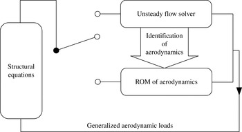
Figure 7 shows a block diagram of FSI modelling. We completed the identification of the aerodynamics and constructed the ROMs in § 3. In this section, we illustrate our direct CFD/CSD simulation method and then focus on constructing ROM-based FSI models by coupling the ROMs with structural motion equations. Validation and verification of the methodology are also conducted.
Block diagram of the FSI modelling configuration.

4.1. Direct CFD/CSD simulation method and its validation
The generalized structural model is as follows:
 $$\begin{eqnarray}\unicode[STIX]{x1D648}\boldsymbol{\cdot }\ddot{{\bf\xi}}+\unicode[STIX]{x1D642}\boldsymbol{\cdot }\dot{{\bf\xi}}+\unicode[STIX]{x1D646}\boldsymbol{\cdot }{\bf\xi}=\boldsymbol{Q},\end{eqnarray}$$
where
 ${\bf\xi}$
is the displacement vector;
 $\unicode[STIX]{x1D648}$
,
 $\unicode[STIX]{x1D642}$
and
 $\unicode[STIX]{x1D646}$
are the mass, damping and stiffness matrices respectively;
 $\boldsymbol{Q}$
is the generalized aerodynamic force vector calculated directly by the flow solver proposed in § 2.
The solution of the structural motion equations is often converted into an initial value problem of first-order ordinary differential equations through the state-space method. By defining the structure-state vector
 $\boldsymbol{x}=[{\it\xi}_{1},{\it\xi}_{2},\ldots ,\dot{{\it\xi}}_{1},\dot{{\it\xi}}_{2},\ldots ,]^{\text{T}}$
, the structural equations in state-space form can be expressed as follows:
 $$\begin{eqnarray}\dot{\boldsymbol{x}}=\boldsymbol{F}(\boldsymbol{x},t)=\unicode[STIX]{x1D63C}\boldsymbol{x}+\unicode[STIX]{x1D63D}\boldsymbol{Q}(\boldsymbol{x},t),\end{eqnarray}$$
where
 $$\begin{eqnarray}\unicode[STIX]{x1D63C}=\left[\begin{array}{@{}cc@{}}\mathbf{0} & \unicode[STIX]{x1D644}\\ -\unicode[STIX]{x1D648}^{-1}~\unicode[STIX]{x1D646} & -\unicode[STIX]{x1D648}^{-1}~\unicode[STIX]{x1D642}\end{array}\right],\quad \unicode[STIX]{x1D63D}=\left[\begin{array}{@{}c@{}}\mathbf{0}\\ \unicode[STIX]{x1D648}^{-1}\end{array}\right].\end{eqnarray}$$
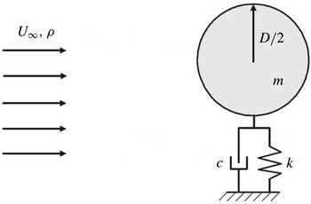
We mainly investigated the dynamics of a one-degree-of-freedom transversely vibrating cylinder (figure 8). Therefore, the structural motion equations can be simplified as follows:
 $$\begin{eqnarray}\ddot{h}+4{\rm\pi}F_{s}{\it\zeta}{\dot{h}}+(2{\rm\pi}F_{s})^{2}h=\frac{2C_{L}}{{\rm\pi}m^{\ast }},\end{eqnarray}$$
where
 ${\it\zeta}$
is the structural damping coefficient. The reduced natural frequency is defined as
 $F_{s}=f_{s}D/U_{\infty }$
and the mass ratio as
 $m^{\ast }=4m/({\rm\pi}{\it\rho}D^{2})$
, where
 $f_{s}$
is the natural frequency of the cylinder,
 $m$
is the actual mass of the oscillator per unit length and
 ${\it\rho}$
is the density of the fluid. Here,
 $\ddot{h}$
,
 ${\dot{h}}$
and
 $h$
denote the normalized acceleration, velocity and displacement of the cylinder in the cross-flow direction. The transverse displacement and velocity of the circular cylinder are normalized by
 $D$
and
 $U_{\infty }$
. In particular,
 $U^{\ast }=1/F_{s}$
is defined as the reduced velocity.
Schematic of a one-degree-of-freedom transversely vibrating cylinder.

A loosely coupled solution algorithm based on CFD simulation in the time domain is employed in this paper to solve the nonlinear FSI problems (Zhang, Jiang & Ye Reference Zhang, Jiang and Ye2007). This algorithm only needs to solve the aerodynamic loads once at each physical time step. The fourth-order hybrid linear multi-step (HLM) scheme is as follows:
 $$\begin{eqnarray}\left.\begin{array}{@{}c@{}}\boldsymbol{Q}_{n}=\boldsymbol{Q}(\boldsymbol{x}_{n},t_{n}),\\ \boldsymbol{F}_{n}=\unicode[STIX]{x1D63C}\boldsymbol{x}_{n}+\unicode[STIX]{x1D63D}\boldsymbol{Q}_{n},\\ \displaystyle \tilde{\boldsymbol{x}}_{n+1}=\boldsymbol{x}_{n}+\frac{{\rm\Delta}t}{24}(55\boldsymbol{F}_{n}-59\boldsymbol{F}_{n-1}+37\boldsymbol{F}_{n-2}-9\boldsymbol{F}_{n-3}),\\ \tilde{\boldsymbol{Q}}_{n+1}=4\boldsymbol{Q}_{n}-6\boldsymbol{Q}_{n-1}+4\boldsymbol{Q}_{n-2}-\boldsymbol{Q}_{n-3},\\ \tilde{\boldsymbol{F}}_{n+1}=\unicode[STIX]{x1D63C}\tilde{\boldsymbol{x}}_{n+1}+\unicode[STIX]{x1D63D}\tilde{\boldsymbol{Q}}_{n+1},\\ \displaystyle \boldsymbol{x}_{n+1}=\boldsymbol{x}_{n}+\frac{{\rm\Delta}t}{24}(9\tilde{\boldsymbol{F}}_{n+1}+19\boldsymbol{F}_{n}-5\boldsymbol{F}_{n-1}+\boldsymbol{F}_{n-2}).\end{array}\right\}\end{eqnarray}$$
The time responses of the coupled system at a given reduced velocity can be calculated directly through the proposed direct CFD/CSD simulation method. Moreover, a few characteristics of VIV, such as the frequency lock-in regime, vibration amplitude of the cylinder and aerodynamic loads, can also be acquired. However, direct numerical simulation of VIV alone is often insufficient to address complex physics and is far too computationally expensive to be utilized in various multi-disciplinary settings, including control model synthesis, multi-variable optimization and stability prediction (Lucia, Beran & Silva Reference Lucia, Beran and Silva2004). Thus, we only use the CFD/CSD simulation method to validate the conclusions analysed by linear dynamics models.
To ascertain the accuracy of our direct CFD/CSD numerical method and its implementation, the VIV of an elastically mounted cylinder in two dimensions was simulated at a low Reynolds number (
 $Re=100$
). The cylinder was free to vibrate in both the transverse and in-line directions, with a low non-dimensional mass ratio (
 $m^{\ast }=10$
). The reduced velocity
 $U^{\ast }(1/F_{s})$
was varied by changing the reduced natural frequency of the cylinder.
The effect of the mesh resolution and far-field boundary location was investigated first here. The
 $F_{s}=0.196$
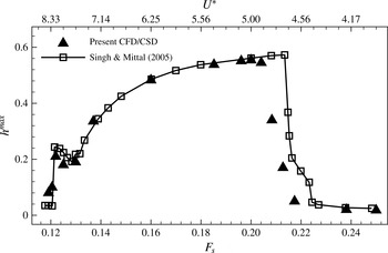
case was chosen for the study, as it is associated with close to maximum vibration amplitude of cylinder (figure 9). The details of the hybrid mesh and a summary of the results calculated are shown in table 3. Meshes M12k and M21k have the same domain size. However, the spatial resolution of M21k is higher, especially close to the cylinder. Mesh M26k has comparable spatial resolution to mesh M21k but has a larger domain size. It can be seen that all of the results are in good agreement. This reflects the adequacy of mesh M21k in computing these FSI problems.
Mesh convergence study: details of the hybrid meshes and summary of the calculated results.

Transverse vibration amplitude of the cylinder as a function of the reduced natural frequency.

Oscillation frequency of the cylinder as a function of the reduced natural frequency.

Given that the amplitude of the transverse vibrations is much higher than that of the in-line oscillations, we only show the results of the transverse vibrations of the cylinder. Figure 9 shows the variation in the transverse displacement of the cylinder with the reduced natural frequency. The cylinder begins to exhibit large-amplitude oscillations at
 $F_{s}\sim 0.12$
and ceases to do so at
 $F_{s}\sim 0.22$
. The maximum vibration amplitude of the cylinder is achieved at approximately
 $F_{s}\sim 0.20$
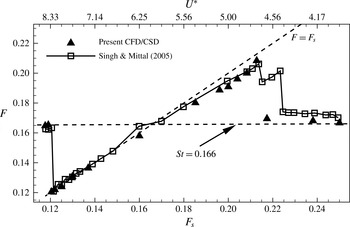
. Figure 10 shows the predominant oscillation frequency (
 $F$
) of the cylinder varying with the reduced natural frequency. When the reduced natural frequency is below 0.12 or above 0.22, the predominant oscillation frequency of the cylinder matches the vortex shedding frequency (
 $F\approx St=0.166$
). The cylinder exhibits forced vibrations under the effect of vortex shedding. However, when the reduced natural frequency is between 0.12 and 0.22, the vibration frequency of the cylinder synchronizes with the reduced natural frequency. Therefore, frequency lock-in occurs. These results were compared with those of Singh & Mittal (Reference Singh and Mittal2005) obtained by increasing
 $U^{\ast }$
. Good agreement was observed. Thus, our direct CFD/CSD simulation method is effective and capable of simulating the frequency lock-in phenomenon in VIV.
4.2. The ROM-based FSI model and its validation
The structure-state vector of a one-degree-of-freedom transversely vibrating cylinder can be expressed as
 $\boldsymbol{x}_{\boldsymbol{S}}=[h,{\dot{h}}]^{\text{T}}$
. The cylinder motion equation (4.4) is transformed into the following state-space form:
 $$\begin{eqnarray}\left.\begin{array}{@{}c@{}}\dot{\boldsymbol{x}}_{\boldsymbol{S}}(t)=\unicode[STIX]{x1D63C}_{\boldsymbol{S}}\boldsymbol{x}_{\boldsymbol{S}}(t)+q\unicode[STIX]{x1D63D}_{\boldsymbol{S}}y_{F}(t),\\ h(t)=\unicode[STIX]{x1D63E}_{\boldsymbol{S}}\boldsymbol{x}_{\boldsymbol{S}}(t)+q\unicode[STIX]{x1D63F}_{\boldsymbol{S}}y_{F}(t),\end{array}\right\}\end{eqnarray}$$
where
 $$\begin{eqnarray}\left.\begin{array}{@{}c@{}}\unicode[STIX]{x1D63C}_{\boldsymbol{S}}=\left[\begin{array}{@{}cc@{}}0 & 1\\ -(2{\rm\pi}F_{s})^{2} & -4{\rm\pi}F_{s}{\it\zeta}\end{array}\right],\quad \unicode[STIX]{x1D63D}_{\boldsymbol{S}}=\left[\begin{array}{@{}c@{}}0\\ 1\end{array}\right],\\ \unicode[STIX]{x1D63E}_{\boldsymbol{S}}=[\begin{array}{@{}cc@{}}1 & 0\end{array}],\quad \unicode[STIX]{x1D63F}_{\boldsymbol{S}}=[0],\quad \displaystyle q=\frac{2}{{\rm\pi}m^{\ast }}.\end{array}\right\}\end{eqnarray}$$
By defining the open-loop state vector
 $\boldsymbol{x}_{\boldsymbol{F}\boldsymbol{S}}=[\boldsymbol{x}_{\boldsymbol{S}},\boldsymbol{x}_{\boldsymbol{F}}]$
and coupling the structural state equations (4.6) with the aerodynamic state equations (3.5), we obtain the state and output equations for the linear coupled system as follows:
 $$\begin{eqnarray}\left.\begin{array}{@{}c@{}}\dot{\boldsymbol{x}}_{\boldsymbol{F}\boldsymbol{S}}(t)=\unicode[STIX]{x1D63C}_{\boldsymbol{F}\boldsymbol{S}}\boldsymbol{\cdot }\boldsymbol{x}_{\boldsymbol{F}\boldsymbol{S}}(t)=\left[\begin{array}{@{}cc@{}}\unicode[STIX]{x1D63C}_{\boldsymbol{S}}+q\boldsymbol{\cdot }\unicode[STIX]{x1D63D}_{\boldsymbol{S}}\unicode[STIX]{x1D63F}_{\boldsymbol{S}}\unicode[STIX]{x1D63E}_{\boldsymbol{S}} & q\boldsymbol{\cdot }\unicode[STIX]{x1D63D}_{\boldsymbol{S}}\unicode[STIX]{x1D63E}_{\boldsymbol{F}}\\ \unicode[STIX]{x1D63D}_{\boldsymbol{F}}\unicode[STIX]{x1D63E}_{\boldsymbol{S}} & \unicode[STIX]{x1D63C}_{\boldsymbol{F}}\\ \end{array}\right]\boldsymbol{\cdot }\boldsymbol{x}_{\boldsymbol{F}\boldsymbol{S}}(t),\\ h(t)=\left[\begin{array}{@{}cc@{}}\unicode[STIX]{x1D63E}_{\boldsymbol{S}} & \mathbf{0}\end{array}\right]\;\boldsymbol{\cdot }\,\boldsymbol{x}_{\boldsymbol{F}\boldsymbol{S}}(t).\end{array}\right\}\end{eqnarray}$$
The ROM-based FSI model for an elastically suspended cylinder is then obtained. The aeroelastic stability problem is converted into solving and analysing the eigenvalues of
 $\unicode[STIX]{x1D63C}_{\boldsymbol{F}\boldsymbol{S}}$
. The real part of the eigenvalue represents the growth rate of the eigenmode, whereas the imaginary part of the eigenvalue corresponds to the circular frequency, which is equal to
 $2{\rm\pi}$
times the eigenfrequency of the eigenmode.
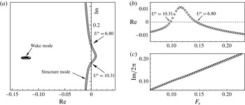
Stability analysis of an elastically suspended cylinder at a subcritical Reynolds number of 33 was conducted to validate the ROM-based FSI model. The cylinder was free to vibrate in the transverse direction. Figure 11 shows the root loci of the coupled system varying with the reduced natural frequency
 $F_{s}$
for
 $m^{\ast }=50$
. The two instability boundaries predicted by the ROM-based FSI model are
 $U_{lower}^{\ast }=6.80$
and
 $U_{upper}^{\ast }=10.31$
. This result is confirmed by direct CFD/CSD simulations (figure 12), where the time histories of the reduced velocities near the onset of instabilities are compared. The time responses calculated by the ROM-based FSI model are in good agreement with those simulated by the direct CFD/CSD method (for small vibrating amplitudes).
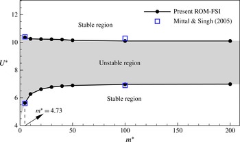
Figure 13 shows the influence of the mass ratio on the instability boundaries of the coupled system. Good agreement with the results of Mittal & Singh (Reference Mittal and Singh2005) is observed at two typical mass ratios. Therefore, the proposed linear model is capable of capturing the stability characteristics of VIV at low Reynolds numbers.
Root loci of the coupled system for
 $Re=33$
and
 $m^{\ast }=50$
: (a) root loci versus the reduced natural frequency of the cylinder (
 $F_{s}$
) and (b) real and (c) imaginary parts of the root loci as a function of
 $F_{s}$
.

Comparisons of time responses in the vicinity of two instability boundaries for
 $Re=33$
,
 $m^{\ast }=50$
. (a,c,e) Lower boundary
 $U^{\ast }=6.80$
; (b,d,f) upper boundary
 $U^{\ast }=10.31$
; (a)
 $U^{\ast }=6.29$
, (b)
 $U^{\ast }=9.52$
, (c)
 $U^{\ast }=6.80$
, (d)
 $U^{\ast }=10.31$
, (e)
 $U^{\ast }=7.41$
, (d)
 $U^{\ast }=11.49$
.

Instability boundaries for
 $Re=33$
analysed by the ROM-based FSI model and the results of Mittal & Singh (Reference Mittal and Singh2005) calculated by direct numerical simulations at two typical mass ratios.

Root loci of the coupled system for
 $Re=60$
and
 $m^{\ast }=50$
.

5. Results and discussion
This paper is focused on interpreting the frequency lock-in phenomenon by using elementary linear dynamics. With this purpose in mind, the ROM-based FSI model constructed in § 4.2 is applied to analyse the mechanisms underlying frequency lock-in in VIV at a low Reynolds number of 60. The reduced velocity
 $U^{\ast }$
is varied by changing the reduced natural frequency of the cylinder (
 $F_{s}$
). The cylinder is free to vibrate in the transverse direction and constrained in the in-line direction. In § 5.1, eigenvalue analysis of the ROM-based FSI model is conducted, and two lock-in patterns are identified, namely ‘resonance-induced lock-in’ and ‘flutter-induced lock-in’. In §§ 5.2 and 5.3, the effects of the mass ratio
 $m^{\ast }$
and the structural damping coefficient
 ${\it\zeta}$
respectively are investigated. In addition, direct CFD/CSD simulations are performed to validate the results analysed by the linear dynamics model.
5.1. Elementary mechanism of frequency lock-in
Linear stability analysis of VIV for
 $Re=60$
was performed based on the ROM-based FSI model. The mass ratio was fixed at
 $m^{\ast }=50$
, and the structural damping coefficient was assigned a zero value (
 ${\it\zeta}=0$
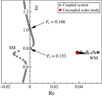
). Figure 14 shows the eigenvalues of the coupled system varying with the reduced natural frequency of the cylinder (
 $F_{s}$
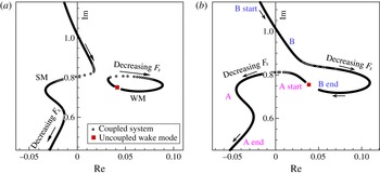
). Two neutral very unstable modes of interest exist, namely the ‘nearly structural mode’ (referred to here as the structure mode, SM) and the ‘von Karman mode’ (referred to here as the wake mode, WM), following the terminology introduced by Cossu & Morino (Reference Cossu and Morino2000) and Meliga & Chomaz (Reference Meliga and Chomaz2011). The WM is absolutely unstable for
 $Re=60$
, whereas the SM is stable at low reduced natural frequency conditions where the interaction between the SM and the WM is weak. However, as the reduced natural frequency of the cylinder approaches the vortex shedding frequency, the FSI becomes strong. Finally, the SM also becomes unstable at certain natural frequencies (
 $0.133<F_{s}<0.166$
). Therefore, the SM and WM become unstable simultaneously at
 $0.133<F_{s}<0.166$
. From the perspective of the real parts of the eigenvalues, the growth rate of the WM is much higher than that of the SM. However, we know that the WM quickly reaches the saturated state because of nonlinearity, whereas the SM, which is essentially linear, only shows nonlinearity because of the interaction with the WM. The instability of the SM, which may play an important role in the frequency lock-in of VIV, is elaborated in the following sections.
(a) Real part, (b) imaginary part of the root loci as a function of the reduced natural frequency of the cylinder and (c) vibration frequency of the cylinder varying with the reduced natural frequency calculated by the direct CFD/CSD simulation method.

Phenomena and principles at different frequency intervals. Here,
 $F_{s}$
is the natural frequency of the cylinder,
 $F_{w}=0.135$
is the saturated vortex shedding frequency of a fixed cylinder for
 $Re=60$
and
 $F_{w-l}=0.12$
is the eigenfrequency of the uncoupled WM for
 $Re=60$
analysed by the linear model.

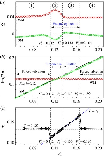
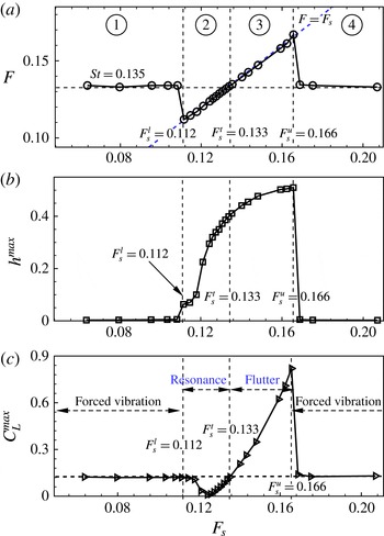
Figure 15(a,b) shows the real and imaginary parts of the root loci in figure 14 as a function of the reduced natural frequency of the cylinder (
 $F_{s}$
). Figure 15(c) plots the reduced vibration frequency of the cylinder (
 $F$
) computed by the direct CFD/CSD simulation method as a function of the reduced natural frequency. Comparison of figures 15(a) and 15(c) shows that the upper instability boundary of the SM predicted by the ROM-based FSI model agrees well with the upper frequency boundary of the lock-in regime computed by the direct CFD/CSD method; both agree at approximately
 $F_{s}^{u}=0.166$
. The lower instability boundary of the SM (
 $F_{s}^{t}=0.133$
) analysed by the ROM-based FSI model and the lower frequency boundary of lock-in (
 $F_{s}^{l}=0.112$
) calculated by the direct CFD/CSD simulations can also be obtained from the figure.
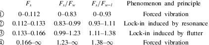
For a more detailed study of frequency lock-in mechanisms in VIV, the reduced natural frequency of the cylinder was divided into four intervals, namely intervals 1, 2, 3 and 4 (figure 15). The four intervals were divided by three critical reduced natural frequencies, namely the lower boundary of frequency lock-in computed by direct CFD/CSD simulations (
 $F_{s}^{l}=0.112$
) and the lower and upper instability frequency boundaries of the SM predicted by the ROM-based FSI model (
 $F_{s}^{t}=0.133$
,
 $F_{s}^{u}=0.166$
). The frequency ranges of the four sections and the corresponding responses of the coupled system and their explanations are listed in table 4. In table 4,
 $F_{w}$
is the dimensionless saturated vortex shedding frequency of a fixed cylinder (i.e. the Strouhal number), defined as
 $F_{w}=St=f_{w}D/U_{\infty }$
. For
 $Re=60$
,
 $F_{w}=St=0.135$
. Here,
 $F_{w-l}$
is the eigenfrequency of the uncoupled WM, which is generally smaller than the saturated vortex shedding frequency
 $F_{w}$
. For
 $Re=60$
, the eigenfrequency of the uncoupled WM analysed by our unsteady aerodynamic model is
 $F_{w-l}=0.12$
, which is consistent with that obtained by Barkley (Reference Barkley2006) from linear stability analysis of the base flow.
For intervals 1 and 4, the cylinder oscillation frequency follows the vortex shedding frequency (
 $F\approx F_{w}=0.135$
) (figure 15
c). The FSI in these two intervals is very weak because the natural frequency of the cylinder is far from the vortex shedding frequency. The cylinder exhibits forced vibrations under the effect of unsteady aerodynamic loads. For intervals 2 and 3, frequency lock-in is observed. However, their primary induced mechanisms may be different, as can be seen from the real parts of the root loci (figure 15
a). In interval 2, only the WM is unstable. However, the natural frequency of the cylinder is exactly located in the vicinity of the eigenfrequency of the uncoupled WM (
 $0.93<F_{s}/F_{w-l}<1.11$
). The dynamic response characteristics of the coupled system are probably associated with resonance. We define this type of frequency lock-in as resonance-induced lock-in. In interval 3, both the SM and the WM become unstable. The phenomenon of negative damping of the SM is similar to the coupled-mode flutter often mentioned in the case of plunge–pitch instability of aerofoils. However, the flutter in this study is not the classical modal coupling between SMs but the coupling between the SM and the WM. We argue that the coupling flutter between the two unstable modes is the root cause of the occurrence of frequency lock-in outside the resonance region. We define this type of frequency lock-in as flutter-induced lock-in.
(a) Vibration frequency of the cylinder (
 $F$
), (b) vibration amplitude of the cylinder (
 $h^{\mathit{max}}$
) and (c) amplitude of the lift coefficient (
 $C_{L}^{\mathit{max}}$
) varying with the reduced natural frequency of the cylinder.

To verify the correctness of the division of intervals and comprehensively investigate the essential difference between the two proposed lock-in patterns, the response characteristics of the coupled system were studied through the direct CFD/CSD simulation method. The oscillation frequency of the cylinder, the vibration amplitude of the cylinder and the amplitude of the lift coefficient as a function of the reduced natural frequency are shown in figure 16. In the lock-in region, the vibration amplitude of the cylinder increased gradually with the increase in reduced natural frequency. The vibration amplitude in the flutter region was higher than that in the resonance region. The peak vibration amplitude was achieved at a distinctly high frequency ratio of
 $F_{s}/F_{w}=1.23$
rather than at the frequency ratio of
 $F_{s}/F_{w}=1.0$
where the natural frequency of the cylinder synchronizes with the vortex shedding frequency. This phenomenon is difficult to explain from the conventional view of simple resonance, in which the highest vibration amplitude often occurs when the forcing frequency approaches the natural frequency of the structure. However, comparison of figures 15(a) and 16(b) shows that the frequency where the cylinder acquires the maximum oscillation amplitude exactly matches the upper instability boundary frequency of the SM analysed by the linear dynamics model (
 $F_{s}^{u}=0.166$
). Notably, the upper frequency boundary
 $F_{s}^{u}=0.166$
corresponds to the onset reduced velocity
 $U_{onset}^{\ast }=1/F_{s}^{u}=6.02$
of frequency lock-in. Thus, the sharp increase in the vibration amplitude of the cylinder at the onset reduced velocity is essentially due to the instability of the SM.
(a,c) Real part of the root loci for
 $m^{\ast }=100$
and
 $m^{\ast }=10$
respectively; (b,d) amplitude of the lift coefficient (
 $C_{L}^{\mathit{max}}$
) varying with the reduced natural frequency of the cylinder for
 $m^{\ast }=100$
and
 $m^{\ast }=10$
respectively.

Moreover, eigenvalue analysis of the linear model not only pinpoints the upper boundary (
 $F_{s}^{u}=0.166$
) of the frequency lock-in regime but also forecasts that
 $F_{s}^{t}=0.133$
is an important demarcation point, namely the transition point from the resonance-induced lock-in region to the flutter-induced lock-in region. This can be confirmed by the amplitude of the lift coefficient as a function of the reduced natural frequency plotted in figure 16(c). In the resonance-induced lock-in region (
 $F_{s}^{l}<F_{s}<F_{s}^{t}$
), the lift coefficient is attenuated, and the amplitude of the lift coefficient is obviously lower than a value that is close to that of a fixed cylinder. The amplitude of the lift coefficient can reach an extremely low value of 0.014 at a frequency ratio of
 $F_{s}/F_{w}\approx 0.94$
. Meanwhile, in the flutter-induced lock-in region (
 $F_{s}^{t}<F_{s}<F_{s}^{u}$
), the lift coefficient is amplified, and the amplitude of the lift coefficient is distinctly higher than the reference value. The maximum amplitude of the lift coefficient is achieved at
 $F_{s}/F_{w}\approx 1.23$
with a fairly high value of 0.71.
Comparisons of time responses and power spectral density results for two representative reduced natural frequencies: (a–c)
 $F_{s}=0.127$
, (d–f)
 $F_{s}=0.158$
.

Comparisons of vorticity fields for two representative reduced natural frequencies: (a)
 $F_{s}=0.127$
, (b)
 $F_{s}=0.158$
.

To verify this correlation, investigation of two other cases (i.e.
 $m^{\ast }=10$
and
 $m^{\ast }=100$
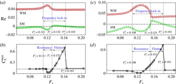
) was carried out and the results are plotted in figure 17. We can see that, for high mass ratios (e.g.
 $m^{\ast }=100$
), the transition frequency predicted by the linear model is clearly related to a value of the lift coefficient close to that for the fixed cylinder. In the resonance-induced lock-in region, the lift coefficient is attenuated. Meanwhile, in the flutter-induced lock-in region, the lift coefficient is amplified. However, for sufficiently low mass ratios (e.g.
 $m^{\ast }=10$
), the transition frequency predicted by the linear model slightly departs from this correlation. This is mainly because the transition frequency is very close to the vortex shedding frequency for the fixed cylinder, where the nonlinear resonance effect becomes stronger at low mass ratios (it is demonstrated that the range of the resonance region increases significantly with decrease of the mass ratio in Govardhan & Williamson (Reference Govardhan and Williamson2000, Reference Govardhan and Williamson2002) and Willden & Graham (Reference Willden and Graham2006)). Therefore, the value of the transition frequency predicted by the linear model may be polluted by the nonlinear resonance effect for low mass ratios. In contrast, the accuracy of the forecast for the upper frequency boundary of lock-in is hardly affected by the mass ratio because it is far away from the vortex shedding frequency for the fixed cylinder. As can be seen, the upper frequency boundaries of lock-in are exactly predicted by the linear model in all cases, which confirms that flutter plays an important role in the phenomenon of frequency lock-in.
To further illustrate the difference between the two lock-in patterns, the responses of two representative reduced natural frequencies (
 $F_{s}=0.127$
and
 $F_{s}=0.158$
) were investigated. Table 4 shows that
 $F_{s}=0.127$
belongs to the resonance-induced lock-in region, whereas
 $F_{s}=0.158$
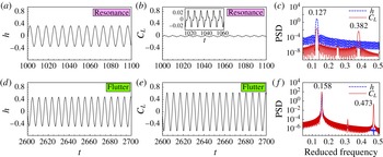
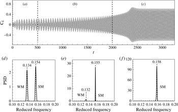
belongs to the flutter-induced lock-in region. The time histories of the transverse displacement of the cylinder and the lift coefficient and the power spectral density results are compared in figure 18. The cylinder oscillation amplitude for
 $F_{s}=0.158$
is slightly higher than that for
 $F_{s}=0.127$
, whereas the lift coefficient for
 $F_{s}=0.158$
is amplified more than 20 times compared with that for
 $F_{s}=0.127$
. The time history of the lift coefficient for
 $F_{s}=0.127$
is detuned, with the existence of a distinctly triple-harmonic frequency. Notably, for
 $F_{s}=0.158$
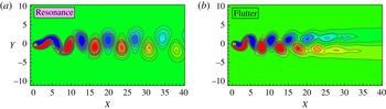
, whose response characteristics are dominated by flutter, the power density of the superharmonic frequency is nearly two orders lower than that of the base frequency. Thus, the time history of the lift coefficient exhibits an almost harmonic response. Figure 19 shows a comparison of the vorticity fields of the two representative reduced natural frequencies. The 2S mode (two single vortices formed per cycle) was observed for
 $F_{s}=0.127$
, whereas the C(2S) mode was observed for
 $F_{s}=0.158$
. The C(2S) mode is very similar to the 2S mode except that the vortices coalesce in the far wake. In the case of
 $F_{s}=0.158$
, the wake begins to coalesce from the fourth to the fifth vortices (figure 19
b). Singh & Mittal (Reference Singh and Mittal2005) obtained similar results in their numerical simulations of VIV at
 $Re=100$
. They explained that the occurrence of the C(2S) mode is due to the high vibration amplitude of the cylinder. However, our numerical simulation results (figure 16
b) show that the vibration amplitude of the cylinder increases slightly from
 $F_{s}=0.127$
to
 $F_{s}=0.158$
, without any discernible change for the division of the 2S mode and the C(2S) mode. Moreover, the type of wake mode may be more relevant to the lift coefficient, as shown in figure 16(c), where the transition point
 $F_{s}^{t}=0.133$
dividing the resonance-induced lock-in region and the flutter-induced lock-in region can be explicitly identified.
Time responses and power spectral density results for different time regimes for
 $F_{s}=0.158$
.

In particular, the linear dynamics shows that both the SM and the WM are unstable in the flutter-induced lock-in region. Thus, how the two unstable modes develop is an interesting question. Figure 20 shows the time history of the lift coefficient and the power spectral density at different time stages for
 $F_{s}=0.158$
. A vigorous competition exists between the two unstable modes. In the initial development stage of the coupled system, the two unstable modes coexist, and a beat phenomenon occurs. The reduced beating frequency analysed from the time response is 0.0204 (for
 $t<500$
), which is slightly higher than that predicted by the ROM-based FSI model, with a value of
 $F_{w}^{couple}\times F_{s}^{couple}=0.121\times 0.155=0.0188$
, where
 $F_{w}^{couple}$
is the eigenfrequency of the WM and
 $F_{s}^{couple}$
is the eigenfrequency of the SM measured from figure 15(b). However, with increase in the vibration amplitude, the SM gradually dominates the dynamics of the coupled system and ultimately causes the vortex shedding frequency to become ‘locked-in’ to the vibration frequency of the cylinder and close to the natural frequency of the cylinder. This result gives further evidence that the instability of the SM is one of the root causes that leads to frequency lock-in in VIV.
5.2. Effect of mass ratio
The mass ratio is known to have an important effect on the damping and frequency characteristics of a coupled system. Section 5.1 indicates that the linear dynamics model can accurately predict the upper frequency boundary of lock-in (
 $F_{s}^{u}$
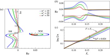
). However, this model has difficulty in predicting the lower frequency boundary of lock-in, which is obviously captured by nonlinear dynamics. We still set the structure damping coefficient to zero and investigated the effects of the mass ratio on the dynamic characteristics of the coupled system. Figure 21(a) shows the root loci of different mass ratios for
 $Re=60$
. The real parts of the SM and the WM in the unstable region are both enlarged with decrease in the mass ratio, which may lead to widening of the synchronization regime. Figure 21(b,c) shows the real and imaginary parts of the root loci. With decrease in the mass ratio, the frequency range of flutter-induced lock-in gradually moves to a high-frequency region (figure 21
b); this indicates that the lock-in phenomenon may occur at extremely large reduced natural frequencies. Furthermore, the eigenfrequency of the SM gradually departs from the unity line
 $F=F_{s}$
with decreasing mass ratio. For the case of
 $m^{\ast }=10$
, the deviation at
 $F_{s}=0.158$
is approximately
 ${\rm\Delta}F=0.024$
, as shown in figure 21(c).
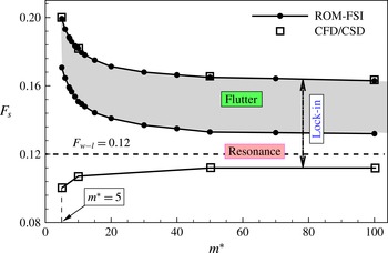
Figure 22 shows the frequency lock-in boundary analysed by the ROM-based FSI model. Surprisingly, good agreement is observed with those calculated by direct CFD/CSD numerical simulations at four representative natural frequencies. With decrease in the mass ratio, the frequency range of resonance-induced lock-in increases rapidly, whereas that of flutter-induced lock-in decreases slightly. However, the upper frequency boundary where flutter may occur increases significantly. Thus, the underlying mechanism of frequency lock-in at high frequency ratio (for
 $m^{\ast }=5$
, the highest frequency ratio reaches
 $F_{s}^{u}/F_{w}=1.66$
) is coupled-mode flutter. The constant line
 $F_{w-l}=0.12$
is located right in the middle of the resonance region. Therefore, resonance-induced lock-in is more relevant to the eigenfrequency of the uncoupled WM.
Root loci of the coupled system at different mass ratios: (a) root loci versus reduced natural frequency
 $F_{s}$
, (b) real and (c) imaginary parts of the root loci.

Frequency lock-in boundaries as a function of mass ratio.

Root loci for two representative mass ratios: (a)
 $m^{\ast }=10$
, (b)
 $m^{\ast }=5$
.

Meliga & Chomaz (Reference Meliga and Chomaz2011) found that at certain parameter settings (
 $Re$
,
 $m^{\ast }$
), no distinction can be made between the WM and the SM because eigenvalue coalescence occurs and both branches exchange roles through a critical mass. A similar phenomenon was observed in our eigenvalue analysis results for the coupled system at low mass ratios for a supercritical Reynolds number of 60. Figure 23 shows the root loci for two representative mass ratios (i.e.
 $m^{\ast }=10$
and
 $m^{\ast }=5$
). Figure 24 shows the corresponding real and imaginary parts as a function of the reduced natural frequency of the cylinder. For the case of higher mass ratio (
 $m^{\ast }=10$
), the SM and WM can be easily identified. Meanwhile, for the case of lower mass ratio (
 $m^{\ast }=5$
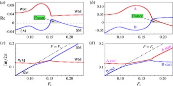
), no distinction can be made between the SM and the WM. The two branches in figures 23(b) and 24(b) are defined as branch A and branch B respectively. When the natural frequency of the cylinder is sufficiently high (the cylinder is nearly rigidly supported), the frequency of branch B is very close to the natural frequency of the cylinder. Therefore, branch B exhibits the SM. Simultaneously, branch A exhibits the WM for the frequency, and the damping of branch A is very close to that of the uncoupled WM. However, with decrease in the natural frequency of the cylinder, the eigenvalue of branch B approaches the eigenvalue of the uncoupled WM, whereas the frequency of branch A approaches the natural frequency of the cylinder. Therefore, branches A and B exchange roles during decrease in the natural frequency of the cylinder. In this case, the critical mass ratio for the occurrence of mode conversion is
 $m_{cr}^{\ast }=7.3$
. It is notable that, for very low mass ratios, frequency conjugating of the two unstable modes is observed when the natural frequency of the cylinder approaches that of the uncoupled wake mode. This kind of solution is similar to the analysis results of De Langre (Reference De Langre2006), in which he referred to this phenomenon as coupled-mode flutter.
Real and imaginary parts of root loci for two representative mass ratios: (a,c)
 $m^{\ast }=10$
, (b,d)
 $m^{\ast }=5$
.

5.3. Critical structural damping coefficient
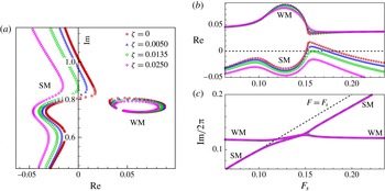
The effect of the structural damping coefficient on the frequency lock-in range was also studied. Figure 25 shows the root loci of the coupled system under different structural damping coefficients for
 $m^{\ast }=10$
. The structural damping coefficient has minimal effect on the frequency and growth rate of the WM. However, the real part of the SM decreases gradually with increase in the damping ratio, that is, the SM tends to become more stable. When the damping ratio is greater than the critical value
 ${\it\zeta}_{cr}$
, the SM becomes absolutely stable and flutter-induced lock-in ceases. The critical structural damping coefficient is 0.0135 for
 $m^{\ast }=10$
.
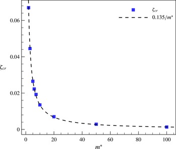
The critical structural damping coefficients for other mass ratios can be acquired in the same manner. Figure 26 shows the critical structural damping coefficient varying with the mass ratio. An approximately inverse correlation exists between the critical structural damping coefficient and the mass ratio:
 ${\it\zeta}_{cr}=0.135/m^{\ast }$
.
Root loci of the coupled system for various structural damping coefficients: (a) root loci versus dimensionless frequency
 $F_{s}$
, (b) real and (c) imaginary parts of the root loci.

Critical structural damping coefficient as a function of the mass ratio.

6. Conclusions
In this study, we investigated the physical mechanisms underlying the frequency lock-in phenomenon in VIV by using a linear dynamics model. The Reynolds number was fixed at 60 and the reduced velocity
 $U^{\ast }(1/F_{s})$
was varied. Two lock-in patterns were identified, and the corresponding frequency ranges were divided through eigenvalue analysis with the ROM-based FSI model. Direct CFD/CSD simulations were also conducted to study the characteristics of the time responses of VIV. The simulation results show that the dynamic responses of the two lock-in patterns exhibit essential differences. This finding confirms the results analysed by the linear dynamics model. The main conclusions can be summarized as follows.
-
(1) Frequency lock-in in VIV at low
 $Re$
can be divided into resonance-induced lock-in and flutter-induced lock-in according to the different underlying mechanisms. When the natural frequency of the cylinder approaches the eigenfrequency of the uncoupled WM (
$0.93<F_{s}/F_{w-l}<1.11$
), the dynamics of the coupled system is dominated by resonance. Meanwhile, at high natural frequencies (
$1.11<F_{s}/F_{w-l}<1.38$
), coupled-mode flutter, manifested by simultaneous instability of the SM and the WM, is the root cause of frequency lock-in.
-
(2) The ROM-based FSI model successfully forecasts the existence of two lock-in patterns and accurately predicts the upper frequency boundary of lock-in. It is indicated that the lock-in of frequency, as well as the sharp increase in the vibration amplitude of the cylinder, occurring at the onset reduced velocity is due to the instability of the SM. This confirms that flutter is one of the root causes of the frequency lock-in phenomenon.
-
(3) The transition frequency of the two lock-in patterns predicted by the ROM-based FSI model is clearly related to a value of the lift coefficient close to that of a fixed cylinder at high mass ratio conditions. In the resonance-induced lock-in region, the lift coefficient is attenuated. Meanwhile, in the flutter-induced lock-in region, the lift coefficient is amplified. However, for very low mass ratio conditions, this correlation is slightly polluted by the strong nonlinear resonance effect.
-
(4) The fundamental mechanism of flutter-induced lock-in is the competition between the two unstable modes. In the initial development stage, both the SM and the WM exist and a beating phenomenon is observed. As time goes on, the dynamics of the coupled system is gradually dominated by the SM, causing the vortex shedding frequency to lock onto the vibration frequency of the cylinder, which is close to the natural frequency of the cylinder.
-
(5) The mass ratio and the mass-damping parameter have an important function in the dynamics of the coupled system. With decrease in the mass ratio, the range of resonance-induced lock-in increases rapidly, whereas the range of flutter-induced lock-in decreases slightly. At sufficiently low mass ratios, frequency lock-in could occur at particular high-frequency ratios (for example, when
$m^{\ast }=10$
,
$F_{s}^{u}/F_{w}=1.66$
). With increase in the damping ratio, the range of flutter-induced lock-in initially decreases and then disappears when the damping ratio is sufficiently large. The critical damping ratio varies inversely with the mass ratio at a fixed Reynolds number. -
(6) Many characteristics of frequency lock-in are associated with linear dynamics. First, the reduced-order model utilized in this study is a linear dynamics model, and the upper frequency boundary of flutter-induced lock-in is precisely predicted compared with that in direct numerical simulations. Second, the linear dynamics model indicates that the resonance-induced lock-in region is located in the vicinity of the eigenfrequency of the uncoupled WM rather than in the vicinity of the nonlinear vortex shedding frequency of a fixed cylinder.




Acknowledgements
The authors gratefully acknowledge the funding of the New Century Program for Excellent Talents of the Ministry of Education of China (NCET-13-0478) and National Natural Science Foundation of China (11572252, 11172237).
Appendix. Nomenclature
-
Important dimensional parameters
-
$m:$
-
mass of the cylinder
-
${\it\rho}:$
-
density of the fluid
-
$D:$
-
diameter of the cylinder
-
$U_{\infty }:$
-
free-stream velocity
-
${\it\upsilon}:$
-
Kinematic viscosity of the fluid
-
$L:$
-
lift force
-
$f:$
-
vibration frequency of the cylinder in the fluid
-
$f_{s}:$
-
natural frequency of the cylinder
-
$f_{w}:$
-
saturated vortex shedding frequency past a fixed cylinder
-
$f_{w-l}:$
-
eigenfrequency of the uncoupled wake mode
-
$f_{w}^{couple}:$
-
eigenfrequency of the wake mode
-
$f_{s}^{couple}:$
-
eigenfrequency of the structure mode
-
Important non-dimensional parameters
-
$m^{\ast }:$
-
mass ratio,
$m^{\ast }=4m/({\rm\pi}{\it\rho}D^{2})$
-
$h:$
-
transverse displacement of the cylinder normalized by
$D$
-
${\it\zeta}:$
-
structural damping coefficient
-
${\it\zeta}_{cr}:$
-
critical structural damping coefficient
-
$C_{L}:$
-
lift coefficient
$C_{L}=2L/{\it\rho}U_{\infty }^{2}D$
-
$Re:$
-
Reynolds number,
$Re=U_{\infty }D/{\it\upsilon}$
-
$St:$
-
Strouhal number,
$St=f_{w}D/U_{\infty }$
-
$F_{s}^{l}:$
-
lower frequency boundary of lock-in
-
$F_{s}^{t}:$
-
transition frequency from resonance to flutter
-
$F_{s}^{u}:$
-
upper frequency boundary of lock-in
-
$U^{\ast }:$
-
reduced velocity,
$U^{\ast }=1/F_{s}=U_{\infty }/f_{s}D$
-
$F,F_{s},F_{w},F_{w-l},F_{w}^{couple},F_{s}^{couple}$
correspond to the non-dimensional forms of
$f$
,
$f_{s}$
,
$f_{w}$
,
$f_{w-l}$
,
$f_{w}^{couple},f_{s}^{couple}$
defined as
$F=fD/U_{\infty }$