





1. Introduction
Since the mid-1990s, mass loss from the Greenland ice sheet (GrIS) has accelerated substantially, contributing an estimated 13.5 mm to global sea level rise from 1992 to 2020 (Otosaka and others, Reference Otosaka2023). A large proportion of this mass loss can be attributed to the dynamic thinning, ungrounding and acceleration of marine-terminating outlet glaciers, which have led to increased ice discharge (Howat and others, Reference Howat, Joughin, Fahnestock, Smith and Scambos2008; Moon and Joughin, Reference Moon and Joughin2008; Straneo and others, Reference Straneo2013; Felikson and others, Reference Felikson2017). The observed changes are partly due to variations in ocean forcing, with the intrusion of warm subsurface Atlantic-origin waters into fjords becoming particularly active in the early 2000s (Holland and others, Reference Holland, Thomas, de Young, Ribergaard and Lyberth2008; Rignot and others, Reference Rignot, Fenty, Menemenlis and Xu2012). This warming, which ranges from ∼1 to ∼3°C (Wood and others, Reference Wood2021), has been explained by the expansion of the Subpolar North Atlantic Gyre, which increased the ocean heat flux into the Irminger and West Greenland currents (Holland and others, Reference Holland, Thomas, de Young, Ribergaard and Lyberth2008). Variations in the fjord heat budget can also arise from large-scale variability in the upper Polar layer (i.e. Arctic-origin waters), especially in West Greenland, where multiple sources of polar water exist from the Baffin and west Greenland currents (Myers and Ribergaard, Reference Myers and Ribergaard2013; Gladish and others, Reference Gladish, Holland, Rosing-asvid, Behrens and Boje2015a, Reference Gladish, Holland and Lee2015b). Subsurface temperatures within these fjords are also known to vary by approximately 0.5–1°C over seasonal timescales (Gladish and others, Reference Gladish, Holland, Rosing-asvid, Behrens and Boje2015a; Carroll and others, Reference Carroll2018; Zahn and others, Reference Zahn2024). The geometry and circulation of fjords play pivotal roles in determining how much of this warm subsurface water reaches the ice fronts of marine-terminating glaciers (Sutherland and others, Reference Sutherland, Straneo and Pickart2014; Straneo and Cenedese, Reference Straneo and Cenedese2015; Catania and others, Reference Catania2018). These waters can enhance calving rates by both weakening the ice mélange through enhanced melting, which reduces the back stress on the ice front, and directly increasing submarine melt at the terminus (Holland and others, Reference Holland, Thomas, de Young, Ribergaard and Lyberth2008; O’Leary and Christoffersen, Reference O’Leary and Christoffersen2013; Catania and others, Reference Catania, Stearns, Moon, Enderlin and Jackson2020).
Given the substantial role of subsurface ocean temperatures in driving GrIS mass loss, combined with fjord geometry and circulation controlling the exchange of water with the shelf, direct measurements of water properties near ice fronts are essential (Straneo and Heimbach, Reference Straneo and Heimbach2013). However, obtaining measurements in these fjords is logistically challenging due to ice mélange, iceberg calving, sea ice and harsh weather conditions, making data collection via moorings, research vessels and Conductivity, Temperature, Depth (CTD) profiles extremely difficult (Fenty and others, Reference Fenty2016; Mankoff and others, Reference Mankoff, Straneo, Cenedese, Das, Richards and Singh2016). While advances have been made in recent decades, such as the Oceans Melting Greenland (OMG) project (Fenty and others, Reference Fenty2016), which acquired in situ ocean measurements in many of Greenland’s fjords, as well as other studies conducting multi-year monitoring (e.g. Straneo and others, Reference Straneo2010, Reference Straneo, Hamilton, Stearns and Sutherland2016; Mortensen and others, Reference Mortensen2013, Reference Mortensen2022; Carroll and others, Reference Carroll2018; Zahn and others, Reference Zahn2024), observations of fjord water properties remain sparse, particularly before the mid-2000s (Snow and others, Reference Snow, Straneo, Holte, Grigsby, Abdalati and Scambos2021). Furthermore, the continuous monitoring of fjord systems remains expensive and logistically challenging. This leads us, and others (e.g. Snow and others, Reference Snow, Straneo, Holte, Grigsby, Abdalati and Scambos2021), to consider whether there are alternative unutilised remote sensing data available that might provide insights into decadal changes in ocean forcing at the ice-sheet’s marine-terminating margins.
In this study, we establish an optimised Landsat-derived sea surface temperature (SST) algorithm for Greenland coastal waters and investigate whether remotely sensed surface temperatures of buoyant subglacial meltwater plumes can serve as a proxy for subsurface ocean temperature variation. These plumes originate from surface meltwaters that reach the ice bed through crevasses and moulins and eventually exit at the grounding lines of marine-terminating outlet glaciers (Chu, Reference Chu2014). Due to their lower density compared to the warm, salty, Atlantic-origin waters found at the bottom of fjords, the plumes rise buoyantly, entraining ambient fjord waters as they ascend (Fig. 1). The volume of the plume can increase by 80 times the initial subglacial discharge as it rises, depending on the depth of the fjord and volume of subglacial water discharged, with the plume’s water properties shifting to reflect the ambient waters it has risen through and entrained (Mortensen and others, Reference Mortensen2013; Mankoff and others, Reference Mankoff, Straneo, Cenedese, Das, Richards and Singh2016; Slater and others, Reference Slater2022). Depending on the fjord’s depth, vertical temperature structure and magnitude of subglacial discharge, these plumes can reach the surface as a visible sediment-laden plume pool (e.g. Mankoff and others, Reference Mankoff, Straneo, Cenedese, Das, Richards and Singh2016; Schild and others, Reference Schild, Hawley and Morriss2016; How and others, Reference How2019; Fig. 1). Thus, the surface temperatures of these plumes may provide insights into the temperatures of the subsurface waters entrained during ascent.
Schematic of a deep (>400 m) Greenland fjord during the peak melt season, featuring a marine-terminating glacier with a surfacing subglacial meltwater plume.

1 Long description
A marine-terminating glacier on the left, with a subglacial discharge flowing downward. This discharge leads to a buoyant meltwater plume, depicted in brown, rising towards the surface. The plume is shown interacting with the surrounding water, causing entrainment, indicated by arrows. Above the plume, ice melange is present. The water body is divided into three layers: the mixed surface layer at the top, the cold polar water in the middle and the warm Atlantic water at the bottom. A Landsat satellite is positioned above, observing the scene. The diagram highlights the interaction between the glacier, meltwater and ocean layers.
This study combines modelling, remote sensing and in situ observations to assess whether plume surface temperatures can serve as indicators of subsurface ocean temperature variability. First, we use a buoyant plume model to theoretically examine the key drivers of plume surface temperature. Second, we develop a method for determining plume surface temperatures from remote sensing using data from Landsat satellites (freely available on the Google Earth Engine platform; Gorelick and others, Reference Gorelick, Hancher, Dixon, Ilyushchenko, Thau and Moore2017; Crawford and others, Reference Crawford2023), which have included thermal infrared bands for measuring the thermal radiance of the Earth’s surface since the launch of Landsat 4 in 1982. We create an open-source Google Earth Engine-based SST retrieval method, specifically optimised for use in Greenland coastal waters and validate it against in situ surface temperature data. Third, we apply this method to extract a time series of plume surface temperatures at Sermeq Kujalleq (Store Glacier) in West Greenland from 1985 to 2024. Finally, we compare these Landsat-derived temperatures with four ocean reanalysis models and modelled plume surface temperatures, forced by CTD profiles collected near the glacier terminus, to contextualise the retrieved signal and explore its potential use as a proxy for changes in subsurface ocean temperature.
2. Methods
2.1. Buoyant plume model
To investigate the physical drivers influencing the surface temperature of buoyant subglacial meltwater plumes (hereby referred to as ‘plumes’), we used a buoyant plume model from Slater and others (Reference Slater, Goldberg, Nienow and Cowton2016). This model simulates the dynamic properties of a line plume (including plume width, temperature, salinity and vertical velocity), as it rises and interacts with ambient fjord waters. We used an initial plume width at the grounding line of 250 m. We applied the model in two ways: (1) to examine the drivers of plume surface temperature and (2) to assess whether modelled and Landsat-derived plume surface temperatures are of a consistent order of magnitude, by forcing the model with in situ CTD profiles collected close in time and space to the Landsat measurements.
2.1.1. Model set-up for investigating drivers of plume surface temperature
To investigate the factors influencing plume surface temperatures, we forced the buoyant plume model with ship- and aircraft-deployed CTD profiles from the OMG project (Fenty and others, Reference Fenty2016) to simulate plumes rising under a variety of fjord conditions. We used profiles compiled by Mas e Braga and others (Reference Mas e Braga, Cowton, Slater, Inall, Johnstone and Fraser2025), who filtered the OMG dataset to retain only profiles within fjords (rather than on the shelf) and removed those visually identified as being in the plume pool. We then applied further quality-control steps to remove profiles containing unphysical or erroneous data caused by sensor issues or sampling artefacts. Profiles were discarded if they contained physically implausible data (temperatures above 8°C or salinities above 40 psu), had a maximum depth shallower than 300 m, or contained salinity or density spikes exceeding three standard deviations from a 10 m moving mean over depth. This filtering discarded 21 profiles (Fig. S2), leaving 99 profiles (Fig. S1), spanning 2016–2021 and distributed around the majority of Greenland’s marine-terminating margins (Fig. S3).
Due to the lack of constraints on the entrainment coefficient, subglacial discharge and depth of the plume origin, we ran the plume model as an ensemble. For each CTD profile, we conducted 40 simulations, sampling model parameters using a Latin hypercube, a statistical sampling method which ensures the entire range of each parameter is representatively sampled. The parameters we varied were the entrainment coefficient (0.05–0.15, Kimura and others, Reference Kimura, Holland, Jenkins and Piggott2014), subglacial discharge (1.25–1250 m3 s−1, Slater and others, Reference Slater2022) and a multiplication factor (0.6–1.4) applied to the maximum depth of each CTD profile (and thus altering the plume origin depth). CTD profiles were extended from their maximum observation depth to the plume origin depth by holding the deepest measured value constant.
Using the results from the buoyant plume model ensemble simulations as training data, we investigated the drivers of plume surfacing (the point at which the plume reaches the ocean surface) and plume surface temperature through a random forest-based sensitivity analysis using scikit-learn (Pedregosa and others, Reference Pedregosa2011). This allowed us to quantify the relative importance of each input variable across all ensembles. Two separate random forest models were fitted for (1) plume surfacing and (2) plume surface temperature using the following variables: subglacial discharge, entrainment coefficient, grounding line depth, mean fjord water temperature of the bottom, middle and top thirds of the water column, and the maximum and mean stratification (using the Brunt–Väisälä frequency, Eqn (1)):
 \begin{equation}{N^2} = {\text{ }}\frac{{ - g}}{{{\rho _{ref}}}}\frac{{d\rho }}{{dz}}\end{equation}
where  $g$ is the acceleration due to gravity,
 $\rho $ is the seawater density and
 $z$ is the depth. The reference seawater density (
 ${\rho _{{\text{ref}}}}$) was taken as the density at the bottom of the profile. We quantified the relative importance of each variable by its contribution to reducing the prediction error using the mean decrease in impurity, where higher values indicate a stronger influence on the model outcome (plume surfacing and plume surface temperature).
2.1.2. Model set-up for comparison to Landsat-derived plume surface temperatures
To provide physical context for the Landsat-derived plume surface temperatures (Section 2.5), we forced the buoyant plume model with available CTD profiles collected near Sermeq Kujalleq (Store Glacier; Section 2.4) to investigate whether the Landsat-derived temperatures are physically consistent with the ambient fjord water column. We screened all CTD profiles from the OMG programme (Fenty and others, Reference Fenty2016) and other literature sources with open-access data, selecting only the profiles taken within 1 month of a Landsat-derived plume surface temperature measurement. Due to frequent cloud cover, the limited temporal and spatial coverage of ice-front proximal CTD profiles and the conditions needed for the plume to surface, the number of matching points was extremely limited; as a result, only three (all from OMG airborne CTD profiles) were used. These profiles ranged from 5 to 20 days from the Landsat-derived SST retrieval date. Moorings in Uummannaq Bay from Carroll and others (Reference Carroll2018) showed a variability of ∼0.5°C at depths of ∼340 m during the summer months. Therefore, we acknowledge that fjord conditions likely evolved over this 5–20 day period; however, these profiles represent the only data available for comparison.
Similar to the model set-up for investigating the drivers of plume surface temperature, the model was run in an ensemble with 100 simulations per profile, with the model parameters sampled randomly using a Latin hypercube. The entrainment coefficient was varied from 0.05 to 0.15 (Kimura and others, Reference Kimura, Holland, Jenkins and Piggott2014). Subglacial discharge estimates were derived from the nearest ice outlet from Mankoff and others (Reference Mankoff2020) and varied from 60 to 140%. This was done to account for uncertainties in runoff catchment size and to ensure plume-surface emergence in some ensemble members. The grounding line depth (depth of plume origin) was varied between 350 and 550 m, spanning the range of grounding line depths near the most frequent plume surfacing location at Sermeq Kujalleq (Store Glacier) (Fig. 9a; Ryan and others, Reference Ryan2015). CTD profiles were extended from their maximum observation depth to the grounding line depth by holding the deepest measured value constant.
2.2. Landsat-derived Arctic SSTs
Investigation of decadal changes in plume surface temperature requires SST data with sufficient spatial resolution to resolve plume pools (∼100 m), optimised for Greenland coastal waters and spanning multiple decades to capture long-term variability in subsurface ocean conditions. The Landsat archive is well-suited for this purpose, as its thermal infrared bands provide the best long-term high-resolution record (∼100 m) available, extending back to the launch of Landsat 4 in 1982. Coarser resolution sensors, such as MODIS, cannot resolve plume pools. Although the widely used Landsat Level-2 surface temperature product from the United States Geological Survey (USGS) offers a long record, it is based on broad land surface temperature relationships and is not directly applicable to marine environments (Cook and others, Reference Cook, Schott, Mandel and Raqueno2014). Existing published Landsat algorithms are likewise not optimised for Greenland coastal waters and typically use split-window methods that are only implementable on the newer Landsat 8 and 9 satellites. Therefore, we developed a dedicated SST algorithm, applicable across Landsat 4, 5, 7, 8 and 9 (providing data from 1982 to present) and optimised for Greenland coastal waters, as outlined below.
To estimate SST using the Landsat archive, we utilised the top-of-atmosphere brightness temperatures from the thermal infrared bands of Landsat 4, 5, 7, 8 and 9 satellites spanning from the launch of Landsat 4 in 1982 through 2024. These data, provided by the USGS, are openly accessible through the Google Earth Engine platform (Gorelick and others, Reference Gorelick, Hancher, Dixon, Ilyushchenko, Thau and Moore2017). We specifically used Landsat Collection 2, Tier 1 data, which contains scenes which have been radiometrically and geometrically calibrated (Crawford and others, Reference Crawford2023) and are of the highest data quality. The nominal spatial resolution of the thermal infrared bands varies between sensors (Table 1), with all bands resampled by the USGS to a uniform resolution of 30 m, which was used throughout this study.
Summary of the Landsat satellites and thermal infrared bands used in this study, along with their corresponding wavelengths, spatial resolutions and K 1 and K 2 calibration constants from the USGS data user’s handbook.

Table 1 Long description
Satellite and sensor entries list a thermal band name, wavelength in micrometers, nominal spatial resolution in meters, and calibration constants K1 in watts per square meter per steradian per micrometer and K2 in kelvin. Landsat 4 Thematic Mapper, Band 6 has wavelength 10.40 to 12.50, nominal spatial resolution 120, K1 671.62, and K2 1284.30. Landsat 5 Thematic Mapper, Band 6 has wavelength 10.40 to 12.50, nominal spatial resolution 120, K1 607.76, and K2 1260.56. Landsat 7 Enhanced Thematic Mapper Plus, Band 6 low gain has wavelength 10.40 to 12.50, nominal spatial resolution 60, K1 666.09, and K2 1282.71. Landsat 8 Thermal Infrared Sensor, Band 10 has wavelength 10.60 to 11.19, nominal spatial resolution 100, K1 774.8853, and K2 1321.0789. Landsat 9 Thermal Infrared Sensor, Band 10 has wavelength 10.60 to 11.19, nominal spatial resolution 100, K1 799.0284, and K2 1329.2405.
To calculate SST, we used a single-channel algorithm with coefficients specifically tuned to the coastal waters of Greenland. SST is commonly retrieved from a linear regression of satellite brightness temperature against surface temperature, with an additional term correcting for atmospheric absorption, which is dominated by the water vapour content of the atmosphere (Merchant, Reference Merchant, Kuenzer and Dech2013). This correction is typically achieved using two thermal infrared bands at different wavelengths (the split-window approach), where the difference in brightness temperature between the ∼11 and ∼12 µm channels is approximately proportional to the impact of atmospheric water vapour absorption and thus serves as a proxy for water vapour absorption (Llewellyn-Jones and others, Reference Llewellyn-jones, Minnett, Saunders and Zavody1984; Merchant, Reference Merchant, Kuenzer and Dech2013). Such split-window methods are only applicable to the Landsat 8 and 9 sensors (e.g. Vanhellemont, Reference Vanhellemont2020); thus, SST retrieval over multiple decades using the older Landsat 4, 5 and 7 satellites (with only one thermal infrared band) requires a single-channel algorithm. Single-channel approaches are well suited to the Arctic, where the cold, dry atmosphere both weakens the 11–12 µm signal that split-window methods rely on and limits water vapour absorption of surface-emitted radiance (Llewellyn-Jones and others, Reference Llewellyn-jones, Minnett, Saunders and Zavody1984). Vincent (Reference Vincent2019) found that single-channel retrieval performed moderately better than split-window techniques under these conditions. For a single channel method, water vapour absorption can instead be accounted for using an external estimate of the total column water vapour, allowing the atmospheric correction to be inferred from a linear regression of the brightness temperature and total column water vapour. The single-channel algorithm we used was a linear regression following an approach similar to that of Snow and others (Reference Snow2025) and took the form:
 \begin{equation}{\text{SST}} = A{T_{\text{b}}} + B\left( {{\text{TCWV}}} \right){T_{\text{b}}} + C + D\end{equation}
where  ${T_{\text{b}}}$ is the brightness temperature of the thermal infrared band (∼10.4–12.5 µm; Table 1), and TCWV is the total column water vapour extracted from the MERRA-2 reanalysis model (Gelaro and others, Reference Gelaro2017), taken from the time step closest to the Landsat acquisition (within ±1 hour) and bilinearly resampled onto the Landsat scene.
 $A,{\text{ }}B$ and
 $C$ are sensor-specific coefficients derived from radiative transfer simulations. Coefficient
 $A$ is the slope, relating the brightness temperature to the surface temperature,
 $B$ corrects for the reduction in the observed brightness temperature caused by water vapour absorption of surface-emitted radiance and
 $C$ is the regression intercept.
 $D$ is a bias correction term derived from the validation process (Section 2.3) that represents the systematic offset caused by residual biases in the MERRA-2 skin temperature and water vapour estimates, the cool-skin effect (Donlon and others, Reference Donlon2002) and systematic errors in the radiative transfer simulations. Similar bias correction terms are applied in coefficient-based SST retrievals to account for residual differences between retrievals and reference observations, which often arise from several sources that are difficult to separate (e.g. Le Borgne and others, Reference Le Borgne, Roquet and Merchant2011; Merchant and others, Reference Merchant, Le Borgne, Roquet and Legendre2013).
2.2.1. Radiative transfer simulations
The algorithm coefficients, A, B and C, must be derived before the algorithm can be applied to real Landsat scenes. To achieve this, we used radiative transfer simulations to model how thermal radiation emitted by the sea surface is absorbed by the atmosphere before reaching the satellite sensor. We conducted radiative transfer simulations using the open-source libRadtran model (v2.0.6; Mayer and Kylling, Reference Mayer and Kylling2005; Emde and others, Reference Emde2016) with modelled atmospheric profiles and sea skin temperature from the MERRA-2 reanalysis model (Gelaro and others, Reference Gelaro2017), following a similar approach to other studies (Vanhellemont, Reference Vanhellemont2020; Guo and others, Reference Guo2025; Snow and others, Reference Snow2025). We specifically used MERRA-2 because it is currently the only reanalysis model with total column water vapour estimates available on the Google Earth Engine platform for the timespan of the Landsat 4, 5, 7, 8 and 9 missions. After calibration, this allowed the Landsat SST retrieval to be entirely conducted within an open-source, cloud-based Google Earth Engine environment.
We extracted 12 800 atmospheric profiles and coincident modelled sea skin temperatures from MERRA-2, sampled spatially across coastal waters within 30 km of the Greenland coastline (Fig. S4). Temporal sampling covered the melt season (May to September) from 1985 to 2025. This sampling ensured that a wide range of typical Arctic atmospheric conditions was sampled (Fig. S4). For each atmospheric profile, the model was forced using the MERRA-2 skin SST and vertical profiles of pressure, temperature and relative humidity. Simulations were run at nadir-viewing geometry, a reasonable approximation given the near-nadir viewing angles of Landsat satellites (Vanhellemont, Reference Vanhellemont2020). The upwelling thermal radiance at the top of the atmosphere was modelled across the 9.8–13.0 µm wavelength range, covering all Landsat thermal bands. Sensor-specific band-averaged sea surface emissivity values were derived from the MODIS UCSB seawater emissivity library (Wan and others, Reference Wan, Ng and Dozier1994), resampled to each Landsat thermal band (Table S1), following Vanhellemont (Reference Vanhellemont2020). While sea surface emissivity can be sensitive to the sediment concentration of the water, this effect is minimal for the typical suspended sediment concentrations found in buoyant subglacial meltwater plumes (∼101–102 mg L−1; Schild and others, Reference Schild, Hawley, Chipman and Benn2017). Within this range, the emissivity varies by approximately 10−3, which has a negligible impact on the overall temperature retrieval (Wen-Yao and others, Reference Wen-yao, Field, Gantt and Klemas1987; Wei and others, Reference Wei, Wang, Gong, He and Bai2017).
The top-of-atmosphere spectral radiance output from the libRadtran simulations was convolved with the specific spectral response functions for the thermal bands of Landsat 4, 5 and 7 (Band 6) and Landsat 8 and 9 (Band 10) provided by the USGS. The effective in-band radiance ( ${L_{{\text{band}}}}$) was calculated as:
 \begin{equation}{L_{band}} = {\text{ }}\frac{{{ \smallint}L\left( \lambda \right)R\left( \lambda \right)d\left( \lambda \right)}}{{{\smallint}R\left( \lambda \right)d\left( \lambda \right)}}\end{equation}
where  $L\left( \lambda \right)$ is the modelled radiance for wavelength (
 $\lambda $) and
 $R\left( \lambda \right)$ is the sensor-specific spectral response. The in-band radiance was then converted to an equivalent brightness temperature (
 ${T_{\text{b}}}$) using the inverse Planck function and the K 1 and K 2 calibration coefficients (Table 1) provided by the USGS for the Landsat Collection 2 data:
 \begin{equation}{T_b} = {\text{ }}\frac{{{K_2}}}{{\ln \left( {\frac{{{K_1}}}{{{L_{band}}}} + 1} \right)}}\end{equation}
These radiative transfer simulations generated a large dataset of simulated Landsat brightness temperatures for varying atmospheric profiles and SSTs. This dataset was used to derive coefficients A, B and C for the single-channel algorithm using the scikit-learn linear regression (Pedregosa and others, Reference Pedregosa2011). Prior to regression, both the simulated brightness temperatures and total column water vapour estimates were standardised using the scikit-learn RobustScaler, which subtracts the median and scales by the interquartile range (Pedregosa and others, Reference Pedregosa2011). The scaling parameters for each sensor are listed in Table S2.
2.3. Validation method, optimisation and cloud/ice masks
To validate the accuracy of the Landsat-derived SSTs, we compared them with in situ data points from the EasyCORA dataset (Szekely and others, Reference Szekely, Gourrion, Pouliquen and Reverdin2024) accessed using the EU Copernicus Marine Service. EasyCORA is a global dataset of in situ ocean temperature and salinity measurements that have been statistically and visually quality controlled and is commonly used for data assimilation into ocean reanalysis models. The dataset consists of measurements from multiple platforms, including gliders, profilers, sea mammals and moorings. We excluded in situ data collected from CTD profiles and ferry boxes, as the collection of these data can mix the upper water column, thereby disrupting the near-surface temperature structure. In situ data were additionally filtered to temperatures between −1.8°C (the approximate freezing point of seawater) and 15°C, to ensure that the validation dataset was representative of Greenland coastal and fjord conditions. The Landsat-derived SSTs were filtered to the same range. Although our SST retrieval algorithm (Section 2.2) was specifically tuned for Greenland coastal waters, the scarcity of cloud-free Landsat scenes with coincident in situ data necessitated the expansion of the validation domain. Therefore, we included in situ data for a pan-Arctic region (here defined as >60°N) spanning from 1982 (launch date of Landsat 4) to 2024 with temperature measurements in the surface water layer at depths of 0–3 m.
The Landsat 4, 5, 7, 8 and 9 collections were filtered to find all scenes that matched each in situ data point location within ±3 hours of the measurement time. Before extracting the SST, we masked each scene using the quality assessment band generated by the CFMask algorithm (Zhu and Woodcock, Reference Zhu and Woodcock2012; Foga and others, Reference Foga2017), retaining only pixels flagged as water (Bit 7) and not flagged as dilated cloud, cloud, cloud shadow or snow (Bits 1, 3, 4 and 5). For Landsat 8 and 9, cirrus flags were additionally applied. The mean SST was then extracted within a 100 m buffer of each in situ data point, provided that at least five valid pixels were present to reduce noise from masked edges. In total, 11 752 matching Landsat scenes and in situ data points were found across Landsat 5–9, with no matches obtained for Landsat 4.
The in situ SST measurements represent the bulk surface temperature from depths of a few centimetres to 3 m depth. In contrast, the Landsat-derived SST represents the skin temperature within the top 10 µm of the water. Under sustained solar irradiance and low wind speeds, skin temperature can deviate by more than 3°C from the bulk temperature (Minnett and others, Reference Minnett2019; Jia and others, Reference Jia, Minnett and Luo2023). To minimise this skin-bulk temperature deviation, we only retained matchups with wind speeds greater than 6 m s−1, calculated using the ERA5 reanalysis model (Hersbach and others, Reference Hersbach2020). This wind speed threshold was chosen following Donlon and others (Reference Donlon2002), who showed that above this threshold, the deviation between the bulk and skin sea temperatures becomes approximately constant and is therefore easier to account for.
Cloud detection algorithms perform poorly in Arctic regions because of the similar multispectral signatures of snow/ice terrain and cloud pixels (Stillinger and others, Reference Stillinger, Roberts, Collar and Dozier2019), leading to many Landsat-derived SST retrievals with cloud and ice contamination. The effect of cloud and ice contamination was reflected in the residual (between Landsat-derived and in situ SST) distributions, which exhibited heavy tails and large excess kurtosis (values of 6–11; Fig. S5) across all sensors, consistent with a small population of heavily contaminated matchups rather than physically meaningful SST variability (Fig. S5). Therefore, we filtered out these outliers by removing points more than one standard deviation away from the mean of the residuals between the Landsat-derived and in situ SSTs in post-processing.
The relationship between the Landsat-derived and in situ SSTs exhibited a residual systematic error. This offset represents a cumulative bias resulting from uncertainties in the MERRA-2 atmospheric data (specifically skin temperature and TCWV), libRadtran simulations and the inherent cool-skin deviation between the Landsat and in situ data (Donlon and others, Reference Donlon2002). To correct for this, we derived a sensor-specific bias correction coefficient D by calculating the mean residual bias between the Landsat-derived and in situ SSTs using 5-fold cross-validation to ensure that the data used to derive D remained independent from those used to assess algorithm performance. D showed minor variation between folds (standard deviation of less than 0.01°C), and residuals between Landsat-derived and in situ SST showed no systematic temperature dependence (Fig. S6), indicating that the bias was approximately constant across the SST range. The coefficient was calculated separately for each Landsat sensor, with Landsat 4 assigned the same value as Landsat 5, which carries an identical sensor, due to an absence of matching in situ observations.
To quantify the performance of the Landsat-derived SSTs, we used several validation metrics based on those recommended for land surface temperature validation by the Committee on Earth Observation Satellites Working Group (Guillevic and others, Reference Guillevic2018). We used the root mean square error (RMSE) to represent the total uncertainty, accounting for both bias and precision errors. Due to the presence of outliers, we used median-based statistics for precision and accuracy. Accuracy was defined as the median absolute residual between the Landsat and in situ measurements, while precision was calculated as the median absolute deviation of the residuals.
2.4. Study site
Sermeq Kujalleq (Store Glacier) is a large marine-terminating outlet glacier located at the head of Ikerasak Fjord near Uummannaq Bay, in West Greenland (Fig. 2). The glacier has a calving front width of 5 km with a grounding line depth which varies from approximately 200–550 m below sea level (Fig. 9a; Ryan and others, Reference Ryan2015), within a fjord that has an average depth of 850 m (Rignot and others, Reference Rignot, Fenty, Xu, Cai and Kemp2015). Due to a basal pinning point, its terminus has remained relatively stable over the past four decades, whereas nearby glaciers have retreated (Howat and others, Reference Howat, Box, Ahn, Herrington and McFadden2010; Todd and others, Reference Todd, Christoffersen, Zwinger, Råback and Benn2019). This stability indicates that the fjord geometry and grounding line depth, and hence their influence on plume surface emergence and temperature, have likely remained constant, making this an ideal site for observing decadal changes in plume surface temperature. The grounding line depth is deep enough to allow warm subsurface Atlantic water to reach the ice front (Chauché and others, Reference Chauché2014). It has been the subject of numerous bathymetric and hydrographic surveys (e.g. Xu and others, Reference Xu, Rignot, Fenty, Menemenlis and Flexas2013; Chauché and others, Reference Chauché2014; Rignot and others, Reference Rignot, Fenty, Xu, Cai and Kemp2015; Fenty and others, Reference Fenty2016), as well as numerous modelling studies (e.g. Xu and others, Reference Xu, Rignot, Fenty, Menemenlis and Flexas2013; Morlighem and others, Reference Morlighem2016; Todd and others, Reference Todd, Christoffersen, Zwinger, Råback and Benn2019; Cook and others, Reference Cook, Christoffersen, Todd, Slater and Chauché2020).
Landsat-derived SST of (a) Sermeq Kujalleq (Store Glacier) on 4 July 2015; the inset shows a zoomed-in Landsat true-colour image of the plume pools. (b) Bathymetry of Uummannaq Bay from BedMachine V5 (Morlighem and others, Reference Morlighem2022) with coloured circles indicating the locations of CTD profiles (yellow) used in Section 3.5 and the extracted data points for the ocean reanalysis models. The inset map of Greenland shows the location of the study area.

Figure 2 Long description
A) A map showing sea surface temperature (SST) in degrees Celsius near Sermeq Kujalleq (Store Glacier) on July 4, 2015. The map includes a zoomed-in inset of plume pools with labeled regions: North, Central and South. Yellow circles indicate CTD profile locations. The scale bar shows 0 to 4 km. B) A bathymetry map of Uummannaq Bay with depth in meters. Colored circles represent ocean reanalysis models: ASTE, ORAS5, TOPAZ4b and EN4. The inset map of Greenland highlights the study area. The scale bar shows 0 to 50 km.
Sermeq Kujalleq (Store Glacier) has plumes that frequently surface adjacent to the ice front. These plumes commonly surface in three separate locations: north, central and south (Fig. 2a). The north plume has an estimated grounding line depth of 400–430 m and the central plume has a depth of 530–550 m. The south plume was not included in the analysis because of the suspected influence of ice marginal runoff.
2.5. Plume surface temperature extraction at Sermeq Kujalleq (Store Glacier)
To extract the surface temperatures of plumes, we used the Google Earth Engine platform to process Landsat scenes spanning from 1982 (the launch date of Landsat 4) to 2024 using our validated SST algorithm. We selected scenes with less than 30% cloud cover, from May to September, a period typically devoid of sea ice and with active subglacial hydrology fed by surface meltwater (Schild and others, Reference Schild, Hawley and Morriss2016). Similar to the validation process, non-water pixels were masked using the quality assessment pixel flags to include only those identified as water and free of cloud, cloud shadow or snow (Section 2.3). Because of the poor performance of cloud detection algorithms in the Arctic regions (Stillinger and others, Reference Stillinger, Roberts, Collar and Dozier2019), each scene was visually quality controlled. Scenes were discarded where cloud cover persisted near the plume pool, where pervasive anomalously low temperatures indicated the presence of thin cirrus cloud transparent in true-colour bands. To be included in the time series, the scenes were required to show a clearly identifiable ice-free plume pool with sufficient valid pixels for reliable temperature extraction. This conservative selection criterion reduces the risk of contaminated retrievals, although we acknowledge that it introduces some subjectivity into scene selection.
Surfacing plumes were visually identified as regions adjacent to the ice front with high sediment content, devoid of ice and sometimes indicated by a well-defined maximum in surface temperature (Fig. 2a; Chu and others, Reference Chu, Smith, Rennermalm, Forster, Box and Reeh2009; Schild and others, Reference Schild, Hawley and Morriss2016). We extracted temperatures for both types of surfacing plumes typically found at marine-terminating glacier margins: (1) those that reach neutral buoyancy at the surface and spread down the fjord and (2) those that reach neutral buoyancy at depth but briefly overshoot to the surface because of their vertical momentum before sinking and spreading at depth (Jouvet and others, Reference Jouvet2018).
We manually extracted plume temperatures by drawing polygons in Google Earth Engine within the area of the plume pool directly adjacent to the ice front, whilst also maintaining a one-pixel buffer from the edge of the plume and ice front to minimise the impact of mixed pixels. By sampling the plume pixels directly adjacent to the ice front, we isolated the active plume region with the strongest upwelling (Mankoff and others, Reference Mankoff, Straneo, Cenedese, Das, Richards and Singh2016; Jackson and others, Reference Jackson2017; Jouvet and others, Reference Jouvet2018; De Andrés and others, Reference De Andrés, Slater, Straneo, Otero, Das and Navarro2020). This approach minimises the influence of horizontal mixing with ambient fjord waters, which has been observed to occur within 500 m of the upwelling point (Jackson and others, Reference Jackson2017).
The Landsat-derived surface temperatures of the plumes were determined by calculating the median values of all extracted pixels. The variability in the plume surface temperature was estimated as the standard deviation and median absolute deviation of all extracted plume pixels. Despite the frequent availability of multiple scenes per year, the occurrence of a cloud-free scene with a visibly surfacing plume remains rare, which limits the number of usable plume surface temperature measurements to 0–9 per year.
From the multi-decadal time series of extracted plume surface temperatures at Sermeq Kujalleq (Store Glacier), we calculated a trend line using Gaussian process regression (Rasmussen, Reference Rasmussen, Bousquet, von Luxburg and Rätsch2004). This regression is well-suited for data with irregular temporal sampling, making it ideal for the intermittent availability of Landsat-derived plume surface temperatures. The central trend was fitted once to all observations with a smoothing length scale fixed at 1.5 years, chosen to capture the multi-year variability while smoothing over seasonal noise. To quantify the uncertainty given sparse, irregular sampling, we bootstrapped this fit 200 times, resampling the observations with replacement and refitting the Gaussian process regression to each sample. The uncertainty bound was taken as the 95% confidence interval of the bootstrap predictions.
2.6. Long-term context using ocean reanalysis data
To contextualise our Landsat-derived plume surface temperatures and compare them to modelled interannual variability and decadal trends at Sermeq Kujalleq (Store Glacier), we utilised modelled monthly ocean temperatures from four different ocean reanalysis products: TOPAZ4b, ASTE, ORAS5 and the EN4.2.2 objective analysis. All data were extracted from the deepest point south of Uummannaq Island at the entrance to Uummannaq Bay (Fig. 2b). This point was chosen because it is the nearest point available in all four models to the ice front of Sermeq Kujalleq (Store Glacier), with the maximum depth of all models being ∼500 m. To represent the variability of subsurface waters entrained into the plume, we used the depth-weighted average ocean temperature at depths between 300 and 500 m.
The reanalysis products differ slightly in horizontal resolution and temporal coverage, and each possesses different biases. Although the model grids are generally too coarse to resolve heat transport into fjords, we used them to characterise broader regional subsurface ocean temperature variability at the entrance to Uummannaq Bay. TOPAZ4b is a coupled ocean and sea ice reanalysis model for the Arctic (Sakov and others, Reference Sakov, Counillon, Bertino, Lisæter, Oke and Korablev2012) provided by the Copernicus Marine Service, providing data at 12.5 km horizontal resolution from 1991 to 2024. Compared with in situ temperature profiles, the model exhibited a slight warm bias of <0.5°C in Baffin Bay (Xie and others, Reference Xie, Bertino, Counillon, Lisæter and Sakov2017). Ocean Reanalysis System 5 (ORAS5) is a global ocean and sea ice reanalysis provided by the European Centre for Medium-Range Weather Forecasts (ECMWF). It provides monthly mean data from 1958 to present and has a horizontal resolution of ∼9 km (Zuo and others, Reference Zuo, Balmaseda, Tietsche, Mogensen and Mayer2019). The Arctic Subpolar gyre state estimate (ASTE) is a coupled ocean-sea ice model with a grid spacing in Baffin Bay of ∼15 km (Nguyen and others, Reference Nguyen, Pillar, Ocaña, Bigdeli, Smith and Heimbach2021) and data availability from 2002 to 2017. A comparison with in situ temperature measurements from Argo floats in the Labrador Sea, which feeds into Baffin Bay, showed that the model matched seasonal and decadal variability well, although it exhibited a cold bias of >0.5°C in the Labrador Sea at depths of 0–500 m (Nguyen and others, Reference Nguyen, Pillar, Ocaña, Bigdeli, Smith and Heimbach2021). The EN4 objective analysis is a monthly gridded dataset of potential temperature and salinity with a horizontal resolution of 1° (Good and others, Reference Good, Martin and Rayner2013). Unlike reanalysis models, EN4 is an interpolation of quality-controlled in situ profiles with a background persistence-based forecast generated from the previous month’s observed ocean state. Because the objective analysis relaxes towards the climatology in the absence of observations, it is susceptible to errors in sparsely sampled regions (Good and others, Reference Good, Martin and Rayner2013).
We applied a 12 month moving average to the ocean reanalysis products to compare them to the interannual variability of the Landsat-derived plume temperatures.
3. Results
In this section, we first use the buoyant plume model to investigate the physical drivers of the plume surface temperatures. We then present the validation results for the Landsat SST algorithm against in situ Arctic SST measurements. Using these Landsat-derived SSTs, we present a 40 year time series of plume surface temperatures at Sermeq Kujalleq (Store Glacier). Finally, we compare the Landsat-derived plume surface temperatures with four ocean reanalysis products and with modelled plume surface temperatures generated by the buoyant plume model forced by near-coincident CTD profiles.
3.1. Relationship between plume surface temperatures, plume surfacing and subsurface temperatures
The dominant control on modelled plume surfacing (whether the plume reaches the ocean surface) is the maximum stratification of the water column (Fig. 3a). This aligns with previous theoretical work (e.g. Jenkins, Reference Jenkins2011), which shows that plumes rise until they reach a neutral buoyancy height, where their density matches that of the ambient water. If the plume retains vertical momentum, it will continue to rise until its vertical velocity decreases to zero. This vertical momentum is primarily determined by the initial buoyancy flux from subglacial discharge at the grounding line. A greater discharge produces a larger initial buoyancy flux, sustaining faster vertical velocities that can overcome ambient density stratification and reduce the rate of dilution due to entrainment, thereby preserving buoyancy (Slater and others, Reference Slater, Goldberg, Nienow and Cowton2016). This physical link between discharge magnitude and upward momentum is consistent with subglacial discharge being the second strongest control on plume surfacing (Fig. 3a). These findings are consistent with those of De Andrés and others (Reference De Andrés, Slater, Straneo, Otero, Das and Navarro2020) at a marine-terminating glacier in West Greenland, where plume surface emergence was found to be primarily controlled by fjord stratification.
Random forest feature importance for (a) plume surfacing and (b) plume surface temperature. Higher values indicate a stronger influence on the random forest model prediction.

For the ensemble members where the plume reaches the surface, the most influential variable for the surface temperature is the mean temperature of the middle third of the fjord, followed by that of the bottom and surface third layers (Fig. 3b). This aligns with buoyant plume theory, where the rate of entrainment of ambient waters into the plume is proportional to its vertical velocity (Morton and others, Reference Morton, Taylor and Turner1956; Jenkins, Reference Jenkins2011). Given that the initial buoyancy flux is greatest at the grounding line, it follows that the plume’s surface temperature is most strongly related to the bottom two-thirds of the water column, where the vertical velocity and entrainment rates are highest (Carroll and others, Reference Carroll2016). The limited influence of the other variables (entrainment coefficient, grounding line depth, fjord stratification and subglacial discharge) further suggests that the plume surface temperature is primarily controlled by the fjord subsurface temperature rather than other dynamical factors.
There is a strong linear correlation between the modelled plume surface temperature and the mean temperature of the middle and bottom thirds of the fjord, with high coefficients of determination (R 2) of 0.97 and 0.93, respectively (Fig. 4a). From a theoretical standpoint, this suggests that more than 90% of the variation in plume surface temperature can be explained by the mean temperature of the bottom two-thirds of the fjord water column, where Atlantic-origin waters are typically found (Chauché and others, Reference Chauché2014; Carroll and others, Reference Carroll2018), with only minor deviations from the linear fit, as indicated by RMSEs of 0.29 and 0.64°C (Fig. 4a). The linear fit suggests that a 0.5°C change in subsurface temperatures is equivalent to ∼0.4°C at the plume surface. The mean plume surface temperature of all the surfacing plume ensembles is 1.03°C, with a median of 0.95°C and an interquartile range of 1.01°C, which provides an estimate of realistic plume surface temperatures expected from the Landsat observations (Fig. 4b). These results demonstrate that the surface temperatures of surfacing plumes are primarily controlled by changes in subsurface ocean temperatures, thereby providing a strong motivation for using remotely sensed plume surface temperatures as a proxy for monitoring subsurface ocean temperature variability.
(a) Scatter plot of the modelled plume surface temperature against the mean bottom and middle third fjord temperatures. (b) Distribution of plume surface temperatures for surfacing ensemble members.

Figure 4 Long description
Scatter plot with the horizontal axis labeled, Bottom or Middle Third Temperature, degree Celsius, ranging from negative 1 to 4. The vertical axis is labeled, Plume Surface Temperature, degree Celsius, ranging from negative 1 to 4. Two point series are shown as separate marker groups, matching the legend entries, Mean Bottom Third Temperature and, Mean Middle Third Temperature. The plotted points form an upward pattern from lower values near negative 1 on both axes toward higher values near 4 on both axes. Text on the plot reads, R2 equals 0.93, RMSE equals 0.64, y equals 0.78x minus 0.19, R2 equals 0.97, RMSE equals 0.29, y equals 0.80x plus 0.11. Histogram with the horizontal axis labeled, Plume Surface Temperature, degree Celsius, ranging from negative 1 to 4. The vertical axis is labeled, Frequency, ranging from 0 to 350. Text on the plot reads, Mean: 1.03 degree Celsius and, Profiles: 2352. A vertical dashed line is drawn at 1.03 on the horizontal axis. The tallest bar is centered near 1 on the horizontal axis, with shorter bars extending toward negative 1 and toward 4. The histogram summarizes the plume surface temperature values shown on the vertical axis of the scatter plot.
3.2. Validation of Landsat-derived Arctic SSTs with in situ data
The accuracy of the Landsat-derived SSTs was evaluated by comparing them with 11 752 pan-Arctic in situ data points from the quality-controlled insitu EasyCORA dataset (Szekely and others, Reference Szekely, Gourrion, Pouliquen and Reverdin2024). For Landsat 4, no matching in situ data were available; however, given that both Landsat 4 and 5 use the same Thematic Mapper sensor, we assumed a comparable performance (Metzler and Malila, Reference Metzler and Malila1985; Ermida and others, Reference Ermida, Soares, Mantas, Göttsche and Trigo2020). The locations of matching points were concentrated in the coastal waters of Norway, Iceland and Svalbard, with 605 validation points within 100 km of the Greenland coast (Fig. 5a). Most of the matching in situ observations were from drifter buoys and moorings (Fig. 5b).
(a) Location of the filtered matching Landsat-derived and in situ SST data points. (b) Frequency of in situ measurement type and Landsat sensor. (c) Frequency of matching in situ data per year for each Landsat sensor.

Figure 5 Long description
A polar map with coastlines and graticule lines. A vertical scale bar at the right is labeled, spatial density, with tick labels 0.25, 0.50, 0.75, 1.00, 1.25, 1.50, 1.75 and a top label 1e minus 3. A label near the upper right reads N colon 11752. The image B showing a stacked bar chart. The horizontal axis label reads Observation Type. Category labels are Buoys, Drifter Buoys, MicroCats, Profilers and Shipboard TSG. A legend at the right lists Landsat, L5, L7, L8 and L9. The vertical axis label reads Frequency. The vertical axis shows tick labels 0, 2000, 4000 and 6000. The stacked bar heights by category are: Buoys, 0; Drifter Buoys, 7000; MicroCats, 5000; Profilers, 0; Shipboard TSG, 0. The image C showing a grouped bar chart by year with multiple series. A legend at the left lists Landsat, L5, L7, L8 and L9. The vertical axis label reads Frequency. The vertical axis shows tick labels 0, 500, 1000 and 1500. The horizontal axis shows years from 1984 through 2023. The plotted values show a tall bar at 2000 reaching 1500 for L7. From 2013 through 2023, multiple bars appear each year for L8 and L9, with heights varying between 0 and about 1500, including several bars near 1000 to 1500 around 2019 to 2021.
Figure 6 shows scatter plots of Landsat 5, 7, 8 and 9 against the corresponding in situ data. As noted in Section 2.3, outliers were filtered out by removing points more than one standard deviation from the mean of the residuals between the Landsat-derived and in situ SSTs. Sea ice, frazil ice, ice mélange and cloud (which were missed by the masks) likely contributed to the large spread of outliers (notably for Landsat 8; Fig. 6b). After applying the sensor-specific bias correction (D, Table 2), the accuracy for each sensor was less than 0.45°C, with a precision within 0.46°C and a total uncertainty (RMSE) below 0.61°C. Previous studies using similar single-channel algorithms reported similar uncertainties when compared to in situ observations (e.g. Tavares and others, Reference Tavares2019).
Validation scatter plots of SST for the whole Arctic region, comparing Landsat-derived SSTs with in situ SSTs from the EasyCORA dataset for (a) Landsat 9, (b) Landsat 8, (c) Landsat 7 and (d) Landsat 5. No matching in situ data were available for Landsat 4. Kernel density estimation (KDE) shows the point density. The legend on each panel shows the validation statistics, derived D coefficient, total number of matching points and number of filtered outliers. Semi-transparent grey points show the outliers removed by the ±1 standard deviation residual filter (Section 2.3). Histograms show the filtered temperature distribution for Landsat (y-axis) and in situ (x-axis) measurements for each sensor.

Figure 6 Long description
A scatter plot titled, Landsat 9. The x-axis is labeled, In-situ SST (degrees Celsius), with tick labels at 0, 2, 4, 6, 8, 10, 12 and 14. The y-axis is labeled, Landsat SST (degrees Celsius), with tick labels at 0, 2, 4, 6, 8, 10, 12 and 14. A diagonal reference line runs from the lower left toward the upper right. A top histogram shows the distribution along the x-axis and a right-side histogram shows the distribution along the y-axis. The plotted points form a narrow diagonal band from near (0, 0) to near (14, 14). A text box inside the plot lists: Arctic; Accuracy equals 0.36 degrees Celsius; Precision equals 0.36 degrees Celsius; Root mean square error equals 0.51 degrees Celsius; D equals 1.15 degrees Celsius; n equals 339; n out equals 5. The image B showing a scatter plot titled, Landsat 8. The x-axis is labeled, In-situ SST (degrees Celsius), with tick labels at 0, 2, 4, 6, 8, 10, 12 and 14. The y-axis is labeled, Landsat SST (degrees Celsius), with tick labels at 0, 2, 4, 6, 8, 10, 12 and 14. A diagonal reference line runs from the lower left toward the upper right. A top histogram shows the distribution along the x-axis and a right-side histogram shows the distribution along the y-axis. Many points form a diagonal band and additional points appear more widely scattered around the band. A vertical color scale at the far right is labeled, KDE Density, with tick labels 0.0, 1.5, 3.1, 4.6, 7.7, 10.8, 12.3 and 13.8 and the text, times 10 superscript 2, near the top. A text box inside the plot lists: Arctic; Accuracy equals 0.35 degrees Celsius; Precision equals 0.39 degrees Celsius; Root mean square error equals 0.53 degrees Celsius; D equals 1.33 degrees Celsius; n equals 8109; n out equals 4074. The image C showing a scatter plot titled, Landsat 7. The x-axis is labeled, In-situ SST (degrees Celsius), with tick labels at 0, 2, 4, 6, 8, 10, 12 and 14. The y-axis is labeled, Landsat SST (degrees Celsius), with tick labels at 0, 2, 4, 6, 8, 10, 12 and 14. A diagonal reference line runs from the lower left toward the upper right. A top histogram shows the distribution along the x-axis and a right-side histogram shows the distribution along the y-axis. The points form a diagonal band with some scattered points away from the band. A text box inside the plot lists: Arctic; Accuracy equals 0.45 degrees Celsius; Precision equals 0.46 degrees Celsius; Root mean square error equals 0.64 degrees Celsius; D equals 0.77 degrees Celsius; n equals 3564; n out equals 2. The image D showing a scatter plot titled, Landsat 5. The x-axis is labeled, In-situ SST (degrees Celsius), with tick labels at 0, 2, 4, 6, 8, 10, 12 and 14. The y-axis is labeled, Landsat SST (degrees Celsius), with tick labels at 0, 2, 4, 6, 8, 10, 12 and 14. A diagonal reference line runs from the lower left toward the upper right. A top histogram shows the distribution along the x-axis and a right-side histogram shows the distribution along the y-axis. The points form a diagonal band from near (0, 0) to near (14, 14), with fewer points than in images B and C. A text box inside the plot lists: Arctic; Accuracy equals 0.45 degrees Celsius; Precision equals 0.44 degrees Celsius; Root mean square error equals 0.61 degrees Celsius; D equals 1.05 degrees Celsius; n equals 3216; n out equals 13.
Single-channel SST algorithm coefficients for each Landsat sensor.

Table 2 Long description
Single channel sea surface temperature algorithm coefficients A, B, C, and D are listed for satellites Landsat 4, Landsat 5, Landsat 7, Landsat 8, and Landsat 9. Landsat 4 has A 3.48, B minus 0.0112, C 275.45, and D 1.049 with an asterisk marker. Landsat 5 has A 3.46, B minus 0.0217, C 275.45, and D 1.049. Landsat 7 has A 3.47, B minus 0.0169, C 275.45, and D 0.769. Landsat 8 has A 3.52, B minus 0.00681, C 275.46, and D 1.328. Landsat 9 has A 3.52, B minus 0.00729, C 275.46, and D 1.152.
Notes: Coefficients A, B and C were derived from libRadtran radiative transfer simulations, and D is a sensor-specific bias correction derived from validation against EasyCORA in situ data (Section 2.3).
* No matching in situ data were available for Landsat 4; D was therefore taken from Landsat 5, which carries an identical sensor.
As our main objective was to create a method for the accurate retrieval of plume surface temperatures for marine-terminating glaciers in Greenland, it is important that the SST retrieval algorithm performs well for Greenland coastal waters. There were 605 validation points available in Greenland’s coastal waters, compared to 11 752 for the pan-Arctic region, mainly associated with Landsat 8 (Fig. 7). For this sensor, the accuracy was 0.44°C, precision within 0.41°C and an RMSE of 0.56°C, comparable to the validation against the full Arctic dataset.
Validation scatter plots of SST for Greenland’s coastal waters comparing Landsat-derived SSTs with in situ SSTs from the EasyCORA dataset for (a) Landsat 9, (b) Landsat 8 and (c) Landsat 7. No matching in situ data were available for Landsat 4 or 5 in this region. Kernel density estimation (KDE) shows the point density. Semi-transparent grey points show the outliers removed by the ±1 standard deviation residual filter (Section 2.3). Histograms show the filtered temperature distribution for Landsat (y-axis) and in situ (x-axis) measurements for each sensor.

Figure 7 Long description
Three scatter plots compare Landsat-derived sea surface temperature with in situ sea surface temperature for Greenland′s coastal waters. The x-axis is labeled ′In situ SST (degree Celsius)′ and the y-axis is labeled ′Landsat SST (degree Celsius)′. Each plot includes a diagonal reference line indicating perfect agreement. In the first plot for Landsat 9, points are mostly clustered along the diagonal, suggesting strong agreement. The text box shows accuracy as 0.42 degree Celsius, precision as 0.39 degree Celsius and RMSE as 0.53 degree Celsius. The second plot for Landsat 8 shows a wider spread of points around the diagonal, indicating more variability. The text box indicates accuracy as 0.44 degree Celsius, precision as 0.41 degree Celsius and RMSE as 0.56 degree Celsius. The third plot for Landsat 7 has fewer points, closely aligned with the diagonal, showing good agreement. The text box lists accuracy as 0.40 degree Celsius, precision as 0.37 degree Celsius and RMSE as 0.50 degree Celsius. Kernel density estimation (KDE) is represented by a color scale, indicating point density, with darker colors showing higher density. Marginal histograms display the temperature distribution for both Landsat and in situ measurements, highlighting the spread and central tendency of the data.
3.3. Spatial temperature structure of surfacing plumes
Figure 8 displays a selection of plumes that are characteristic of those frequently observed during the melt season. Surfacing plumes at Sermeq Kujalleq (Store Glacier) commonly appear as sediment-laden, ice-free plume pools adjacent to the ice front (Fig. 8). The surface temperature of these plume pools appears spatially homogeneous in both the 100 m Landsat 8 and 9 imagery and the higher-resolution 60 m Landsat 7 imagery (Table 1). The within-plume spatial variation in surface temperature is less than 1°C, which is comparable to the uncertainty in Landsat-derived temperatures. When plumes surface at multiple locations along the ice front, their surface temperature differs noticeably, with the north plume being ∼0.6°C warmer than the central plume and ∼2°C colder than the southern plume (Fig. 8c), likely reflecting their different origin depths and varied access to different layers of the water column (Fig. 9). The latter warm southern ‘plume’ is likely influenced substantially by terrestrial runoff.
(a–d) Landsat-derived spatial temperature structure of surfacing plumes at Sermeq Kujalleq (Store Glacier). The left column of each subplot shows the Landsat true-colour scene, and the right shows the Landsat-derived SST. Black polygons show the manually drawn approximate locations of surfacing plumes.

Figure 8 Long description
Each map is oriented with north at the top. The left side of each panel shows true-color imagery, while the right side shows SST. Black polygons outline the approximate locations of surfacing plumes. The temperature scale ranges from -2.0 to 4.0, with cooler temperatures indicated by one end of the scale and warmer temperatures by the other. A) The map from 28th July 2006 using Landsat 7 shows plume locations and temperature variations. B) The map from 11th August 2014 using Landsat 8 highlights changes in plume distribution and temperature. C) The map from 4th July 2015 using Landsat 8 shows further variations in plume extent and temperature. D) The map from 6th August 2014 using Landsat 8 depicts similar features. Across the years, the maps reveal changes in the extent and intensity of temperature anomalies and plume footprints, indicating dynamic environmental conditions at the glacier terminus.
(a) Estimated location along the grounding line of plume surface emergence, using bathymetry from Ryan and others (Reference Ryan2015). Point colours correspond to the number of plumes observed in that location. Red dotted line highlights the onset of the isothermal section of the CTD profile in (c). (b) Histogram of plume origin depth. (c) OMG airborne CTD profile 3.5 km away from the ice front of Sermeq Kujalleq (Store Glacier) on 25 August 2020 (Fenty and others, Reference Fenty2016).

Figure 9 Long description
A scatter plot with a horizontal axis label, Distance Along Icefront North to South, kilometer, ranging from 0 to 5 and a vertical axis label, Depth, meter, ranging from 0 to minus 600. A top axis label reads, Plume occurrence frequency, with tick labels 2, 4, 6, 8, 10, 12. A legend lists, Grounding Line Depth and, Landsat Plume Temperature location. A dashed curve labeled by the legend as Grounding Line Depth starts near left parenthesis 0, 0 right parenthesis, drops steeply to near minus 600 meters close to distance 0, stays near the bottom through the middle distances, then rises toward about minus 200 meters near distance 5. Circular markers labeled by the legend as Landsat Plume Temperature location appear mainly between about minus 300 and minus 600 meters, with several markers near the deepest part around minus 520 to minus 580 meters. Marker positions include approximately left parenthesis 1.0, minus 320 right parenthesis, left parenthesis 1.5, minus 380 right parenthesis, left parenthesis 2.0, minus 420 right parenthesis, left parenthesis 2.5, minus 470 right parenthesis, left parenthesis 3.0, minus 520 right parenthesis, left parenthesis 3.5, minus 560 right parenthesis, left parenthesis 4.0, minus 520 right parenthesis, left parenthesis 4.5, minus 420 right parenthesis and left parenthesis 4.8, minus 300 right parenthesis. A horizontal dotted line crosses at about minus 350 meters. The image B showing a histogram with a horizontal axis label, Frequency, ranging from 0 to 12 and a vertical axis label, Depth, meter, ranging from 0 to minus 600. Horizontal bars are grouped by depth bins. The longest bars reach about 10 to 12 on the Frequency axis and occur in mid depth bins around the horizontal dotted line. Shorter bars appear in shallower and deeper bins. A horizontal dotted line crosses at about minus 350 meters. The image C showing a line graph with a horizontal axis label, Temperature, degree celsius, ranging from 0 to 2.0 with tick labels 0, 0.5, 1.0, 1.5, 2.0 and a vertical axis corresponding to Depth, meter, ranging from 0 to minus 600. The line begins near about 0.2 degree celsius at 0 meters, increases with depth, reaches about 2.0 degree celsius at around minus 350 meters, then stays close to 2.0 degree celsius down to about minus 600 meters. A horizontal dotted line crosses at about minus 350 meters. Across the three graphs, the horizontal dotted line at about minus 350 meters appears in all three, aligning the scatter plot depths, the histogram depth bins and the temperature profile depth where the temperature reaches about 2.0 degree celsius.
3.4. Time series of Landsat-derived plume surface temperatures
Our time series uses Landsat 5, 7, 8 and 9 scenes from 1985 to 2024. Although Landsat 4 scenes were processed from 1982, no scenes with visible surfacing plumes were identified. At Sermeq Kujalleq, plumes frequently surface in three distinct locations: north, central and south (Figs 2a and 8c). We estimated the plume origin depth by comparing the surface emergence location to a profile of the grounding line depth from Ryan and others (Reference Ryan2015) (Fig. 9). For the plume time series, we focused on plumes with an estimated plume origin depth deeper than 380 m, which is below the depth at which Atlantic-origin water has been observed in Ikerasak Fjord (Chauché and others, Reference Chauché2014) and within the approximately isothermal layer of the water column (Fig. 9c). This depth threshold minimises the impact of varying plume origin depths on the surface temperature. As noted previously, the south plume was excluded because of its proximity to the lateral margin (Fig. 2a), where terrestrial runoff and supraglacial meltwater may influence its properties.
Figure 10a shows the Landsat-derived plume surface temperature time series at Sermeq Kujalleq (Store Glacier), derived from Landsat 5, 7, 8 and 9 scenes from 1985 to 2024. The mean plume surface temperature was 1.92°C, with a standard deviation of 0.65°C and a range from −0.02°C to 3.47°C. The regression of the plume surface temperature time series revealed three distinct phases: a cool period from 1985 to 1996 (characterised by high uncertainty in the regression), a warming transition between 1996 and 2002 and a warm phase extending to 2016, followed by a more distinct cooling trend from 2016 to 2023. These phases are in general agreement with the warming of subsurface waters in Disko Bugt in 1997, as reported by Holland and others (Reference Holland, Thomas, de Young, Ribergaard and Lyberth2008) and the general model trends reported by Rignot and others (Reference Rignot, Fenty, Menemenlis and Xu2012), demonstrating that the time series captures the expected decadal trend of subsurface ocean variability. Large seasonal and interannual variability (standard deviation of ∼0.4°C and 0.7°C, respectively), which is comparable to the observed decadal range of ∼1°C, nevertheless complicates the interpretation of the observations.
Plume surface temperature time series for Sermeq Kujalleq (Store Glacier). (a) Landsat-derived plume surface temperatures (circles) are coloured by Landsat sensor, with the error bar representing the standard deviation of the extracted pixels. The solid blue line shows a Gaussian Process Regression, with the shaded region indicating the 95% confidence interval derived from bootstrap resampling (n = 200). (b) Monthly ocean reanalysis model weighted-depth average (300–500 m) temperatures from Uummannaq Bay (Figure 2b) are shown by the thin lines. The solid bold line indicates the 12 month moving mean. The shaded region represents a 12 month rolling standard deviation. The Landsat temperature regression, as reported in (a), is also shown.

Figure 10 Long description
Panel a shows Landsat-derived plume surface temperatures at Sermeq Kujalleq (Store Glacier) from 1985 to 2024. The vertical axis is labeled Temperature (degree C), ranging from 0 to 4. The horizontal axis is labeled Year, ranging from 1985 to 2024. The graph includes circular markers representing Landsat 5, 7, 8 and 9 with error bars indicating the standard deviation. A solid blue line represents a Gaussian Process Regression, with a shaded region showing the 95 percent confidence interval. Notable trends include a cool period from 1985 to 1996, a warming transition between 1996 and 2002 and a warm phase extending to 2016, followed by cooling from 2016 to 2023. Panel b displays monthly ocean reanalysis model temperatures from Uummannaq Bay, with the same axes and ranges. Thin lines represent TOPAZ, ASTE, ORAS5 and EN4 datasets, while a bold line indicates the 12-month moving mean. The shaded region shows a 12-month rolling standard deviation. The Landsat regression from panel a is also shown. Trends include general agreement with warming and cooling phases observed in panel a. The comparison demonstrates variability in temperature estimates across different datasets and highlights the decadal trend of subsurface ocean variability. Key insights include the alignment of warming trends with subsurface water changes in Disko Bugt reported in 1997. Peaks and lows are visible, with notable fluctuations around 2002 and 2016. The purpose of the graph is to compare temperature estimates from different sources and illustrate changes over time.
Comparisons between the Landsat-derived time series and ocean reanalysis models, including the EN4 objective analysis, revealed substantial discrepancies in temperature variability at all timescales, notably including large divergence between the reanalysis models themselves (Fig. 10b). The models do not agree on broad decadal trends in subsurface ocean temperature variability, and their yearly means can differ by >1.5°C, with EN4 (based on in situ profiles) generally displaying warmer temperatures than the ocean reanalysis models. This divergence between models highlights the difficulty in obtaining accurate ocean forcing estimates for Greenland’s marine-terminating glaciers, with coarse-resolution ocean models struggling to resolve heat transfer into fjords (Wood and others, Reference Wood2024). Consequently, this lack of consensus between reanalysis products complicates direct comparisons with our Landsat-derived estimates. Despite this, the reanalysis models and Landsat-derived plume surface temperatures are of the same order of magnitude, although consistent agreement between them in terms of both temperature and trajectory is rare. Figure 11 shows the 4 year sliding Pearson correlation coefficient between the Landsat temperature regression and modelled temperatures. While brief periods of strong positive correlation appear sporadically throughout the time series, they are transient and lack coherence across models, suggesting that they are likely spurious or incidental. Exceptions to this include a period of strong correlation between TOPAZ4b, EN4 and Landsat-derived plume surface temperatures between 2017 and 2019. For TOPAZ4b and Landsat, this strong agreement extends to 2023, with both time series showing a linear (R 2 > 0.87) cooling trend. This decreasing trend with a lower uncertainty on the Landsat regression coincides with the launch of Landsat 8, where an improved thermal infrared sensor (Reuter and others, Reference Reuter2015) and more frequent data points allow for easier identification of possible outliers (e.g. 2016 and 2022).
Four-year sliding Pearson correlation coefficient between the Landsat-derived plume surface temperature regression and a twelve-month rolling mean of (a) TOPAZ4b, (b) ASTE, (c) ORAS5 and (d) EN4 ocean reanalysis models. Positive values >0.7 indicate a strong correlation, and negative values <−0.7 indicate a strong negative correlation.

Figure 11 Long description
The multi-line graph consists of four panels comparing the 4-year sliding Pearson correlation coefficient between Landsat-derived plume surface temperature regression and four ocean reanalysis models: TOPAZ, ASTE, ORAS5 and EN4. The horizontal axis represents the year, ranging from 1988 to 2024. The vertical axis represents the correlation coefficient, ranging from negative 1.0 to 1.0, with reference lines at 0.0, 0.7 and negative 0.7. Panel A shows TOPAZ with a filled area indicating correlation. Peaks occur around 1998 and 2010, with strong positive correlations above 0.7. Negative correlations are seen around 1992 and 2004. Panel B shows ASTE with a filled area. Positive correlations appear around 2008, while negative correlations are seen around 1994 and 2012. Panel C shows ORAS5 with a filled area. Positive peaks occur around 2000 and 2016, with negative correlations around 1996 and 2008. Panel D shows EN4 with a filled area. Positive correlations are seen around 1990 and 2018, with negative correlations around 1994 and 2006. Overall, TOPAZ and EN4 show more consistent positive correlations, while ASTE and ORAS5 display more variability. Each panel uses distinct shading to differentiate the datasets.
The Landsat-derived plume surface temperatures can exhibit large temporal variability within a single year, with years with more than three data points having a mean range of 1.23°C (Fig. 12). This variability is comparable in magnitude to in situ observations at the entrance of Rink Isbrae fjord in Uummannaq Bay from 2013 to 2015. Ocean temperatures at a depth of ∼250 m showed a decrease from June to August of ∼0.5°C, with shallow temperatures increasing by ∼2°C (Carroll and others, Reference Carroll2018; Fried and others, Reference Fried2018). However, our Landsat-derived plume surface temperatures showed no clear seasonality (Fig. 12), and given that the observed range (1.23°C) is only ∼2 times the retrieval uncertainty, it is unclear whether this seasonal variability is genuine.
Seasonal variation of Landsat-derived plume surface temperature (blue) for the 6 years with the most data points. Error bars show the standard deviation of the extracted plume pixels.

Figure 12 Long description
Six line graphs, each representing plume surface temperature in degrees Celsius from July to August for different years: 2024, 2019, 2017, 2016, 2015 and 2001. The x-axis shows the months July and August, while the y-axis represents plume surface temperature ranging from 0 to 3.5 degrees Celsius. Each graph features a line with circular markers indicating data points. For 2024, the temperature fluctuates, peaking around early August. In 2019, the temperature shows a slight increase through the period. The 2017 graph displays a significant dip in late July. In 2016, the temperature decreases steadily. The 2015 graph shows a drop in late July, followed by a rise. In 2001, the temperature remains relatively stable with minor fluctuations. The graphs illustrate how plume surface temperatures vary across these years, highlighting differences in trends and peaks. The purpose is to compare seasonal temperature variations over the specified period.
3.5. Comparison of Landsat-derived and modelled plume surface temperatures
For all Landsat-derived plume surface temperatures at Sermeq Kujalleq (Store Glacier) (Fig. 10), three corresponding OMG CTD profiles were available near the ice front and outside the plume. These OMG CTD profiles sampled the ambient fjord water column and were used as inputs to the buoyant plume mode. The profiles were acquired 5–20 days after the Landsat retrievals and from 1.0 to 7.5 km from the ice front (Fig. 2).
For each of the three OMG CTD profiles, the Landsat-derived plume surface temperatures showed marginal agreement with the modelled plume temperatures, and only when accounting for the uncertainty in the Landsat estimates (Fig. 13). This uncertainty range (calculated in quadrature from the plume pool median absolute deviation and sensor RMSE) overlapped with some of the model ensemble members for all three dates. However, there were large offsets between the median Landsat-derived plume surface temperature and the mean of the modelled plume surface temperature ensembles. These differences are likely due to the 5–20 day gap between each CTD profile and Landsat retrieval, during which fjord conditions can change. Subsurface temperatures can vary by 0.5–1°C over such timescales (Gladish and others, Reference Gladish, Holland, Rosing-asvid, Behrens and Boje2015a; Carroll and others, Reference Carroll2018; Zahn and others, Reference Zahn2024), so the mismatch does not necessarily reflect errors in either method. Additionally, the subsurface temperature between the three CTD profiles differed by only ∼0.5°C (Fig. 13), which, from the relationship presented in Section 3.1, corresponds to only a 0.4°C change at the plume surface. This is smaller than the 0.25–0.5°C spread of the plume ensemble in each panel (Fig. 13) and smaller than the Landsat retrieval uncertainty of ∼0.6°C. Therefore, we do not expect the Landsat-derived estimates to resolve the exact variance or direction of the changes between these specific profiles. However, this comparison demonstrates that the Landsat retrievals capture the correct overall magnitude, with their uncertainty bounds overlapping the modelled ensembles in all three cases, supporting the theoretical relationship established in Section 3.1.
Comparison of CTD-modelled and Landsat-derived plume surface temperatures at Sermeq Kujalleq (Store Glacier) for the three matching cases (a–c). CTD temperature (blue) and salinity (black) profiles, with dotted lines indicating extrapolated values. Landsat-derived plume surface temperatures (orange) with the uncertainty range (quadrature sum of plume pool median absolute deviation and sensor RMSE). Ensemble of modelled plume profiles (grey) and the ensemble mean (black dashed line).

Figure 13 Long description
2016-08-30, t-16 d, 7.46 km. Two adjacent plots share a vertical axis labeled, Depth (m), with tick labels at 0, minus 100, minus 200, minus 300, minus 400, minus 500 and minus 600. Left plot x-axis label, Temperature (degrees Celsius), with tick labels 0, 0.5, 1.0, 1.5, 2.0, 2.5 and 3.0. A blue temperature line starts near about 2.0 at depth 0, moves left to about 1.0 by about minus 100, then continues left to about 0.6 by about minus 200, then turns right to about 1.0 by about minus 300 and reaches about 2.0 to 2.2 by about minus 400 to minus 450, then stays near about 2.0 to 2.2 down to about minus 600. Many thin grey temperature curves form an envelope that is near about 2.0 to 2.5 at depth 0, narrows toward about 0.5 to 1.0 around minus 200 to minus 300, then bends right toward about 2.0 to 2.5 by about minus 400 to minus 600. A black dashed temperature curve runs within the grey envelope, bending similarly and lying near about 2.0 to 2.3 below about minus 400. Right plot x-axis label, Salinity (psu), with tick labels 30, 31 and 32. A black salinity curve lies near about 32 at depth 0 and remains close to 32 down to about minus 600, with a slight leftward bend around roughly minus 100 to minus 300. The image B showing 2019-08-09, t-20 d, 1.03 km. Two adjacent plots share a vertical axis labeled, Depth (m), with tick labels at 0, minus 100, minus 200, minus 300, minus 400, minus 500 and minus 600. Left plot x-axis label, Temperature (degrees Celsius), with tick labels 0, 0.5, 1.0, 1.5, 2.0, 2.5 and 3.0. A blue temperature line starts near about 2.0 at depth 0, moves left to about 1.0 by about minus 100, then to about 0.6 to 0.7 by about minus 200, then turns right to about 1.0 by about minus 300 and reaches about 2.0 to 2.2 by about minus 400 to minus 450, then stays near about 2.0 to 2.2 down to about minus 600. Many thin grey temperature curves form an envelope similar to image A, narrowing around minus 200 to minus 300 and bending right below about minus 350. A black dashed temperature curve runs within the grey envelope and lies near about 2.0 to 2.3 below about minus 400. Right plot x-axis label, Salinity (psu), with tick labels 30, 31 and 32. A black salinity curve lies near about 32 at depth 0 and remains close to 32 down to about minus 600, with a small leftward bend around roughly minus 100 to minus 300. The image C showing 2020-08-20, t-5 d, 3.80 km. Two adjacent plots share a vertical axis labeled, Depth (m), with tick labels at 0, minus 100, minus 200, minus 300, minus 400, minus 500 and minus 600. Left plot x-axis label, Temperature (degrees Celsius), with tick labels 0, 0.5, 1.0, 1.5, 2.0, 2.5 and 3.0. A blue temperature line starts near about 2.0 at depth 0, moves left to about 1.0 by about minus 100, then to about 0.6 by about minus 200, then turns right to about 1.0 by about minus 300 and reaches about 2.0 to 2.2 by about minus 400 to minus 450, then stays near about 2.0 to 2.2 down to about minus 600. Many thin grey temperature curves again form an envelope that narrows around minus 200 to minus 300 and bends right below about minus 350. A black dashed temperature curve runs within the grey envelope and lies near about 2.0 to 2.3 below about minus 400. Right plot x-axis label, Salinity (psu), with tick labels 30, 31 and 32. A black salinity curve lies near about 32 at depth 0 and remains close to 32 down to about minus 600, with a slight leftward bend around roughly minus 100 to minus 300.
4. Discussion
This study successfully developed and validated Landsat-derived SSTs specifically optimised for Greenland’s coastal regions, with data availability spanning from the launch of Landsat 4 in 1982 to present and a retrieval uncertainty of ∼0.6°C. This has allowed for the extraction of a 40 year time series of Landsat-derived plume surface temperatures at Sermeq Kujalleq (Store Glacier), providing a novel dataset for investigating decadal changes in subsurface ocean temperatures at a marine-terminating glacier. The time series of Landsat-derived plume surface temperatures matches the magnitude of the theoretical estimates and shows trends that are broadly consistent with expected decadal variability (Holland and others, Reference Holland, Thomas, de Young, Ribergaard and Lyberth2008; Rignot and others, Reference Rignot, Fenty, Menemenlis and Xu2012).
Although this plume surface temperature time series provides a novel tool for investigating subsurface ocean temperatures, its use as a reliable quantitative proxy remains preliminary. The large seasonal variability (∼1.2°C; Section 3.4) is comparable in magnitude to the decadal variability (∼1°C; Section 3.4), and the lack of reliable validation data makes it challenging to confidently infer subsurface temperature changes. Additionally, retrieval uncertainty means a plume surface temperature change must exceed ∼0.6°C to be resolved, which, based on the linear fit in Fig. 4a, corresponds to a subsurface change of approximately 0.8°C. Consequently, separating genuine subsurface signals from observational noise and external factors (e.g. solar heating or mixing with surface waters) remains challenging.
This ambiguity is compounded by the lack of reliable datasets against which to compare our estimates of plume surface temperatures and inferred subsurface ocean temperature variability. We found that ocean reanalysis models exhibit considerable disagreement in this region, effectively ruling them out as useful comparison tools. Additionally, using CTD profiles as contextual constraints on modelled plume temperatures is severely limited by the scarcity of profiles spatiotemporally coincident with cloud-free Landsat scenes, thereby limiting our ability to explore the physical drivers of observed plume surface temperatures. Therefore, while the current uncertainties and lack of thorough validation preclude the use of the method as a standalone proxy for subsurface warming, this study serves as an initial proof of concept, providing a validated, high-resolution SST retrieval method optimised for Greenland coastal waters. The feasibility of this method may improve with the higher spatial resolution and lower revisit times of next-generation thermal infrared satellites (e.g. TRISHNA; Section 4.5), along with continued community efforts to obtain hydrographic data in Greenland’s fjords. Below, we discuss these validation challenges, the uncertainties and physical processes likely driving the observed variability, recommendations for future work and other possible glaciological applications of high-resolution Landsat SSTs.
4.1. Limitations in validation: data sparsity and disagreement between reanalysis models
Validating Landsat-derived plume surface temperatures for interpreting long-term changes in subsurface temperatures remains challenging. This is primarily due to the sparsity of in situ observations and the inherent uncertainties in translating these profiles into modelled plume surface temperatures. As demonstrated in Section 3.5, the Landsat-derived and modelled plume surface temperatures showed marginal agreement for the three model simulations with temperature inputs from near-coincident CTD profiles. However, this is only when accounting for the large retrieval uncertainty of the Landsat data (Fig. 13). Further uncertainties may stem from limitations in the buoyant plume line models themselves, with recent observations suggesting that these models underrepresent entrainment and volume flux, potentially leading to an underestimation of plume temperature (Ovall and others, Reference Ovall2025).
With only three near-coincident CTD profiles available, it remains unclear whether the Landsat plume surface temperatures genuinely reflect ambient fjord subsurface waters or are more strongly influenced by external factors (e.g. solar heating, mixed pixels and mixing with surface waters). This is exacerbated by the considerable temporal (5–20 days) and spatial (1.0–7.5 km) offsets between the Landsat retrievals and CTD profiles. Over these timescales, variations in subglacial discharge and temperature stratification of the surface layer can change the conditions required for the plume to surface (De Andrés and others, Reference De Andrés, Slater, Straneo, Otero, Das and Navarro2020). Furthermore, fjord subsurface temperatures (the primary control on plume surface temperatures, Section 3.1) can vary by approximately 0.5–1°C over such periods (Gladish and others, Reference Gladish, Holland, Rosing-asvid, Behrens and Boje2015a; Carroll and others, Reference Carroll2018; Zahn and others, Reference Zahn2024). This suggests that hydrographic conditions likely evolved between the Landsat and CTD observations, which is supported by the substantial seasonal variability seen in the Landsat retrievals themselves (mean range 1.23°C; Fig. 12). The spatial offset between the CTD profiles and the ice front introduces some uncertainty, as distant profiles may not fully capture the ambient fjord conditions that the plume rises through. However, subsurface waters exert the biggest control on plume surface temperatures (Section 3.1), and while observations at Sermeq Kujalleq (Store Glacier) by Chauché and others (Reference Chauché2014) highlight that surface-layer temperatures can vary by ∼1.5°C within 10 km of the ice front, their CTD profiles show little variation in water temperature at depth (below ~300 m) from 3 to 20 km away.
Comparing the long-term Landsat-derived plume surface temperature time series with ocean reanalysis products (TOPAZ4b, ASTE, ORAS5 and EN4) presents similar challenges. As demonstrated in Section 3.4, these models exhibit substantial discrepancies in temporal variability and magnitude (Fig. 10). This highlights the inherent difficulty that reanalysis models face in modelling the temperature variability of the water column in Arctic settings (Uotila and others, Reference Uotila2019). While the Landsat trend shows similarities to EN4 and TOPAZ4b (particularly the linear cooling from 2016 to 2023), the lack of consensus across the reanalysis models reflects their limitations as reliable estimates in this region, making it unclear which of the four datasets in Fig. 10 provides the most accurate representation of subsurface ocean temperature variation. Therefore, neither the in situ data nor the diverging reanalysis models currently provide a robust baseline against which to effectively quantify the feasibility of a remotely sensed proxy for subsurface temperature changes. Ultimately, this lack of consensus highlights the need for new observational datasets, such as the remotely sensed proxy explored here, to improve constraints on ocean forcing of the ice sheet.
4.2. Uncertainties in the SST algorithm
The SST algorithm involves a linear regression of the brightness temperature and total column water vapour. The accuracy of this retrieval is constrained by several uncertainties introduced at multiple stages. First, the coefficients,  $A$,
 $B$ and
 $C$ are derived from radiative transfer simulations which rely on atmospheric profiles from the MERRA-2 reanalysis model. Any bias in the MERRA-2 data, particularly in the estimation of the total column water vapour, will propagate directly into the retrieval coefficients. The bias correction coefficient (D) partially mitigates this systematic bias.
Second, the bias correction coefficient (D) was derived by validating against in situ measurements, which sample the bulk water rather than the ∼10 µm skin layer measured by Landsat. These two temperatures differ mainly due to the cool-skin effect, with smaller contributions from near-surface stratification (Donlon and others, Reference Donlon2002; Minnett and others, Reference Minnett2012; Jia and others, Reference Jia, Minnett and Luo2023). Our >6 m s−1 wind speed filter minimises this difference by limiting matchups to well-mixed conditions, but some residual mismatch and uncertainty in D may remain.
Finally, the SST retrieval is ultimately limited by the radiometric performance of the Landsat sensors. This includes artefacts such as electronic noise, thermal striping, thermal band calibration drift and operational anomalies (e.g. the Landsat 7 scan-line corrector failure) (Barsi and others, Reference Barsi, Schott, Hook, Raqueno, Markham and Radocinski2014).
These uncertainties are difficult to minimise and may make it challenging to accurately detect the sub-degree changes in plume surface temperature required to investigate decadal changes in subsurface ocean temperatures. With a Landsat-derived SST retrieval uncertainty of ∼0.6°C, plume surface temperature changes must exceed this value to be resolved. Based on the linear fit of subsurface ambient temperatures and plume surface temperatures in Fig. 4a, this establishes a sensitivity threshold where subsurface temperatures must change by at least ∼0.8°C to be detectable using this method.
4.3. Influence of mixed pixels
The spatial resolution of the thermal bands of Landsat sensors ranges from 60 to 120 m (Table 1), whereas the plume pool at Sermeq Kujalleq (Store Glacier) varies from 0.2 to 2 km2 (∼20–200 pixels). Despite using a one-pixel buffer to minimise the effects of mixed pixels at the edges, the plume pool may still contain residual ice or non-plume water. We assumed that visibly surfacing plumes had sufficiently vigorous upwelling to displace all ice mélange, leaving a clear plume pool, consistent with high-resolution UAV observations (e.g. Jouvet and others, Reference Jouvet2018; Chudley and others, Reference Chudley, Christoffersen, Doyle, Abellan and Snooke2019). However, some ice mélange may persist within the plume pool that is not visible at the spatial resolution of the Landsat imagery. This would result in thermal radiance measurements that average the ice and plume waters, leading to lower surface temperature measurements. Residual cloud cover undetected by the CFMask algorithm could also lead to interference in the plume surface temperature retrieval, with cloud detection algorithms having an accuracy of only ∼80% (Foga and others, Reference Foga2017).
Measurements of horizontal velocities at different depths from Mankoff and others (Reference Mankoff, Straneo, Cenedese, Das, Richards and Singh2016) and UAV-derived surface velocities from Jouvet and others (Reference Jouvet2018) revealed spatially heterogeneous upwelling, with plume-driven upwelling (and thus the arrival of entrained ambient waters) concentrated in a narrow ∼0.03 km2 area. The remaining plume spreads horizontally, potentially mixing with the surrounding near-surface fjord water (Mankoff and others, Reference Mankoff, Straneo, Cenedese, Das, Richards and Singh2016; Jackson and others, Reference Jackson2017; De Andrés and others, Reference De Andrés, Slater, Straneo, Otero, Das and Navarro2020), which could influence its temperature independently of the ambient waters through which it rises. Without UAV-based thermal studies or high-density CTD measurements (e.g. Jackson and others, Reference Jackson2020; Zheng and others, Reference Zheng2021; Savidge and others, Reference Savidge2023), the spatial homogeneity of plume surface temperatures remains uncertain.
4.4. Solar and sensible heating of the plume surface
Solar heating and heat exchange with the atmosphere are known to influence the skin temperature of the ocean surface and are therefore a potential source of variability in Landsat-derived plume surface temperatures. Adiabatic cooling from wind and wind-induced mixing can lower the skin temperature (Minnett and others, Reference Minnett2012; Jia and others, Reference Jia, Minnett and Luo2023), whereas insolation can warm the near-surface layer (Eastwood and others, Reference Eastwood, Le Borgne, Péré and Poulter2011; Snow and others, Reference Snow, Straneo, Holte, Grigsby, Abdalati and Scambos2021). On sub-daily timescales, diurnal warming under low-wind, high insolation conditions can raise the skin temperature by a few degrees, which decreases overnight (Eastwood and others, Reference Eastwood, Le Borgne, Péré and Poulter2011). On seasonal timescales, sustained heat accumulation can raise water temperatures by several degrees, as observed in the terrestrial lakes near Sermeq Kujalleq (Store Glacier), where summer lake temperatures progressively rise over the summer (Fig. S7). However, while such heating significantly impacts stationary, relatively static lake water, the extremely turbulent environment of a vigorously upwelling plume likely mitigates this effect (e.g. Movie S1; Mortensen and others, Reference Mortensen2020). The surface-reaching ensemble members in Fig. 13 typically exhibit vertical velocities exceeding 1 m s−1, rapidly replenishing the surface layer. This magnitude is consistent with direct observations at the LeConte Glacier, Alaska, where near-surface vertical upwelling of >1.1 m s−1 was recorded alongside large horizontal spatial variability (Ovall and others, Reference Ovall2025). Additionally, the large horizontal surface velocities observed at Bowdoin Glacier (Jouvet and others, Reference Jouvet2018) and Saqqarliup Sermia (Mankoff and others, Reference Mankoff, Straneo, Cenedese, Das, Richards and Singh2016) in Greenland emphasise the turbulent nature of the plume pool. This constant mixing results in a short residence time of waters at the plume surface, thereby limiting the influence of solar heating and wind-induced cooling on the observed temperatures.
4.5. Recommendations for future research
The main limitation of using the method developed in this study to infer subsurface temperature variations is the scarcity of CTD profiles collected close in time and space to the Landsat-derived plume surface temperatures at Sermeq Kujalleq (Store Glacier), with only three near-coincident CTD profiles available. Consequently, it remains unclear whether the large observed seasonal variability is a genuine physical signal or an artefact arising from the issues mentioned previously (sensor error, algorithm uncertainties or secondary influences from solar heating and mixing with other water sources). However, future insights are likely to emerge from the next generation of thermal infrared satellite missions with increased sensor accuracy, revisit times and spatial resolution. For example, the commercial HotSat-1 satellite, launched in 2023, provides on-demand thermal measurements at a 3.5 m spatial resolution with a revisit time of 1–2 days. Open-access data will also become available with the launch of TRISHNA (scheduled for 2027), which will provide high-resolution thermal imagery with significantly improved revisit times. These advances, alongside the continued retrievals for Landsat 8 and 9, could allow for a better characterisation of the seasonal variability of plume surface temperatures, which is important for establishing reliable interannual and decadal trends in the data.
In addition to advances in satellite technology, UAV thermal imagery of plume pools could help address the unknowns that currently limit the Landsat method, including the poorly constrained spatial heterogeneity of the plume pool surface temperatures and the magnitude of diurnal and seasonal variability. Coordinated campaigns acquiring UAV imagery coincident with Landsat overpasses would allow for the rigorous validation of Landsat-derived plume surface temperatures. Additionally, pairing these remote observations with coincident in situ CTD profiles near the ice front would enable a thorough exploration of the physical factors driving plume surface temperature variability. This would definitively determine whether variations in subsurface ocean temperatures control variations in plume surface temperature.
It is important to select glaciers that are suitable for investigating remotely sensed plume surface temperatures. Sermeq Kujalleq (Store Glacier) is an ideal study site, due both to the relative decadal stability of its terminus and the frequent plume activity. For the central plume (Fig. 9a), this terminus stability implies that the subglacial portal remains spatially consistent, ensuring that the plume entrains water from a consistent depth within the fjord water column. In addition, unlike at larger marine-terminating glaciers, it lacks extensive mélange cover that often obscures surfacing plumes; however, the fjord is sufficiently deep to enable warm Atlantic waters to access the glacier terminus (Chauché and others, Reference Chauché2014). Therefore, future studies should investigate glaciers with similar properties and characteristics.
Future work should also explore the disparity in plume surface temperatures between marine-terminating glaciers situated in deep versus shallow fjords. Such a comparison could provide insights into fjord hydrography, specifically determining whether the ice front is accessible to warm Atlantic-origin water or whether the plume is restricted to entraining colder Polar water.
4.6. Further potential uses of Landsat-derived SSTs at the ice-ocean interface
While the primary focus of this study was to investigate plume surface temperatures, the high-resolution SST product developed here holds considerable additional value for broader ice-ocean applications. Although the retrieval uncertainty of ∼0.6°C limits our sensitivity in detecting subtle subsurface temperature changes, it is more than sufficient to resolve the strong thermal gradients typical of fjord surface waters.
For example, Fig. 14 shows the Landsat-derived SST of Disko Bugt on 25 August 2019, revealing clearly defined surface circulation patterns and distinct temperature fronts between glacial/ice mélange meltwaters from Ilulissat Fjord and warmer shelf waters. Additionally, localised meltwater from individual icebergs can be observed (see inset of Fig. 14). This spatial variability and detail could be used to support studies of fjord circulation and temperature change, including constraining and validating detailed hydrodynamic modelling studies, such as those using MITgcm (e.g. Davison and others, Reference Davison, Cowton, Sole, Cottier and Nienow2022). Given that glacial fjord surface waters typically show spatial differences in temperature of a few degrees (Figs 8 and 14), such applications would be well within the remit and accuracy of Landsat-derived SSTs.
SST in Disko Bugt on 25 August 2019, derived from Landsat 8, with clouds, ice and land masked. The background is a true-colour Landsat 8 image of the same scene. The inset shows a zoomed-in view showing the detail of iceberg melt.

Figure 14 Long description
A map of Disko Bugt displays sea surface temperature (SST) on 25 August 2019, derived from Landsat 8. The SST is represented in degrees Celsius, with a gradient ranging from -1.0 to 10.0. The map includes a legend indicating temperature ranges. The main map shows a distinct temperature front between glacial meltwaters and warmer shelf waters. An inset provides a zoomed-in view of iceberg melt, highlighting localized meltwater patterns. The map includes a scale bar for distance, marked in kilometers and coordinates for orientation. Clouds, ice and land are masked to focus on water temperatures.
5. Conclusions
We developed an open-source, Google Earth Engine-based SST method with retrieval coefficients optimised for the coastal waters of Greenland. While specifically tuned for these coastal environments, validation against 11 752 in situ measurements demonstrated that the algorithm also performed well across the broader Arctic. Our results show that these Arctic-validated SSTs achieved an RMSE of ∼0.6°C, with an accuracy of ∼0.4°C. These optimised high-resolution SSTs allow for investigations of Greenland’s fjords, coastal regions and ice-ocean interfaces (Section 4.6). Using Landsat-derived SSTs and the theoretical knowledge that changes in subsurface ocean temperatures have a large influence on plume surface temperatures (Section 3.1), we generated a 40 year time series of plume surface temperature changes at Sermeq Kujalleq (Store Glacier) to investigate its potential as a proxy for decadal changes in subsurface fjord temperatures. In doing so, we also provide the first long-term record of plume-surface temperature variability at a marine-terminating glacier.
The retrieved plume surface temperatures align with the magnitude of theoretical estimates and exhibit trends that are broadly consistent with the expected decadal variability of subsurface ocean temperatures. However, confidently inferring subsurface changes remains challenging. Specifically, we found that the magnitude of the observed seasonal variability (∼1.2°C) was comparable to the decadal signal (∼1°C). Additionally, while the 1–3°C of subsurface warming in the early 2000s is believed to have enhanced submarine melt rates (Rignot and others, Reference Rignot, Fenty, Menemenlis and Xu2012; Wood and others, Reference Wood2021), its influence on the plume surface temperature signal was likely minor compared to the uncertainty of the retrieved SST (∼0.6°C) and other sources of plume surface temperature variability (Section 4). This complicates our ability to distinguish genuine subsurface temperature changes from observational noise, retrieval uncertainty and external factors (Section 4.3). Resolving this variability, whether it reflects genuine subsurface ocean temperature changes or secondary influences, is currently constrained by a lack of reliable validation data. Comparisons with ocean reanalysis models revealed substantial inter-model disagreement in this region. While our analysis is limited to a single grid point, the disagreement we found between reanalysis products reflects a wider difficulty in obtaining reliable ocean temperatures near Greenland’s marine-terminating glaciers. Given the importance of ocean warming in driving their retreat, acquiring better estimates of ocean forcing remains a priority for understanding ice-ocean interactions. This highlights the value of exploring new observational methods, such as the approach presented here, to improve our knowledge of ice-ocean interactions, characterise trends in past ocean forcing and better constrain the ocean products used to force the next generation of ice-sheet projections.
Despite these limitations, there are clear signs that an increased temporal resolution can improve the utility of this method. We observed that post-2013, following the launch of Landsat 8, the time series showed less seasonal variability and more coherent interannual trends, suggesting that an increased sampling frequency facilitates more robust outlier detection. Looking forward, further improvements will be made using the next generation of thermal infrared satellites. Emerging commercial platforms (e.g. HotSat-1) and upcoming open-access missions (e.g. TRISHNA; planned for 2027) will provide high spatial resolution and frequent revisit times necessary to capture rapid fjord dynamics. Such observations, combined with continued Landsat retrievals, will be essential for clarifying whether the variability in plume surface temperatures reflects genuine changes in subsurface water properties or arises from other observational uncertainties. To facilitate future work, we have made the retrieval code openly available and developed Google Earth Engine applications, allowing for easy access and utilisation of this optimised SST product (Appendix A).
Supplementary material
The supplementary material for this article can be found at https://doi.org/10.1017/jog.2026.10204.
Data availability statement
The Landsat Collection 2 products data used in this study are freely available from the Google Earth Engine platform, courtesy of the United States Geological Survey. The spectral response functions of each Landsat sensor are available from the USGS spectral characteristics viewer (https://landsat.usgs.gov/spectral-characteristics-viewer). The EasyCORA in situ temperature dataset (Szekely and others, Reference Szekely, Gourrion, Pouliquen and Reverdin2024) is available through the EU Copernicus Marine Service In Situ Thematic Assembly Centre: https://doi.org/10.17882/46219. MERRA-2 atmospheric profiles are available from: https://doi.org/10.5067/QBZ6MG944HW0 and skin surface temperature from: https://doi.org/10.5067/VJAFPLI1CSIV. The TOPAZ4b Arctic Ocean Physics Reanalysis are available from the EU Copernicus Marine Service Information: https://doi.org/10.48670/moi-00007. ORAS5 model data, prepared by the ECMWF, are available from: https://doi.org/10.24381/cds.67e8eeb7. ASTE model data are available at the Arctic Data Center: https://arcticdata.io/data/10.18739/A2CV4BS5K/. The EN4.2.2.g10 objective analysis data are available at: https://www.metoffice.gov.uk/hadobs/en4/download-en4-2-2.html. The Oceans Melting Greenland AXCTD and CTD profiles are available from OMG (2020). Supporting data of the libRadtran simulations, validation matchups between in situ and Landsat-derived SST, and plume surface time series data at Sermeq Kujalleq (Store Glacier) are available at: https://doi.org/10.5281/zenodo.20607849. The code used to derive, validate and optimise the Landsat SST algorithm is available at: https://doi.org/10.5281/zenodo.20610026. The code used to conduct the plume modelling and analyse and plot the plume surface temperature time series is available at: https://doi.org/10.5281/zenodo.21822805. Example code of how to retrieve Landsat-derived Arctic SSTs, the Google Earth Engine web app (Appendix A) and documentation are available at: https://github.com/ry-ing/arctic-landsat-sst-GEE.
Acknowledgements
R.I. was supported by a UK Natural Environment Research Council PhD studentship (NE/T00939X/1). D.S. acknowledges support from NERC Independent Research Fellowship NE/T011920/1. P.N. and E.M.-L. were supported by NERC Grant NE/X01536X/1.
Author contributions
R.I. led the development of the SST method, modelling and analysis, under the supervision of P.N., D.S. and E.M.-L. R.I. led the preparation of the manuscript, with input from all authors.
Appendix A Landsat-derived Arctic SST web apps
We have additionally developed a web app (Fig. A1) that allows users to download Landsat SST scenes using the Greenland-optimised SST algorithm for specified dates and regions (https://github.com/ry-ing/arctic-landsat-sst-GEE). The app uses USGS Landsat Collection 2 data and is a Google Earth Engine-based web app. Also available is the plume surface temperature extraction app that allows users to download CSV files of plume surface temperatures for each available Landsat scene.
Google Earth Engine web app for interactive viewing of Greenland-optimised Landsat-derived SSTs.

Figure A1 Long description
A thematic map in a Google Earth Engine app displays Landsat-derived Arctic sea-surface temperature (SST). The map shows an island-dense coastline on the right and open ocean on the left. Exact location is not labeled. The map lacks a legend, scale and north arrow, limiting interpretability. The SST pattern is visible with smooth gradients over the ocean and irregular patches over land. Warmer SST areas appear in certain ocean regions, while cooler areas are elsewhere. No place names are shown. The interface includes controls for cloud cover percentage, date selection and SST visualization range. An inspector tool shows SST as 9.32 degrees Celsius. The map′s purpose is to visualize SST distribution, highlighting warmer and cooler regions in the Arctic. Orientation is not indicated.
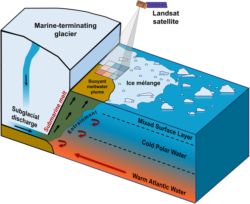

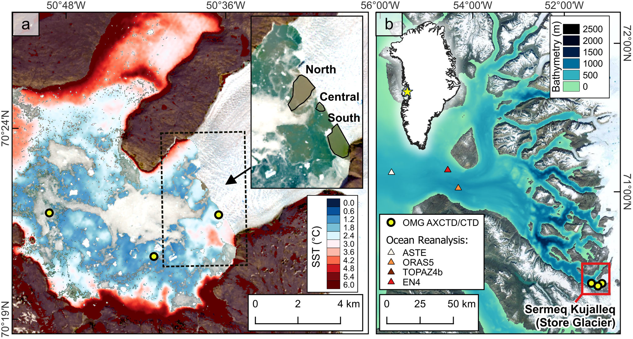
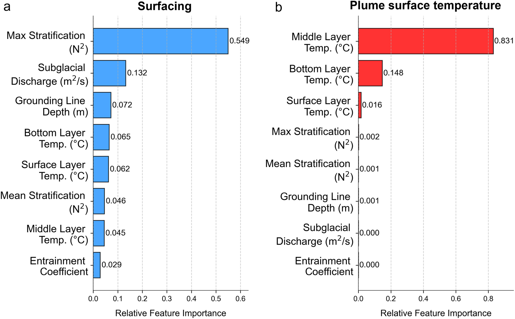
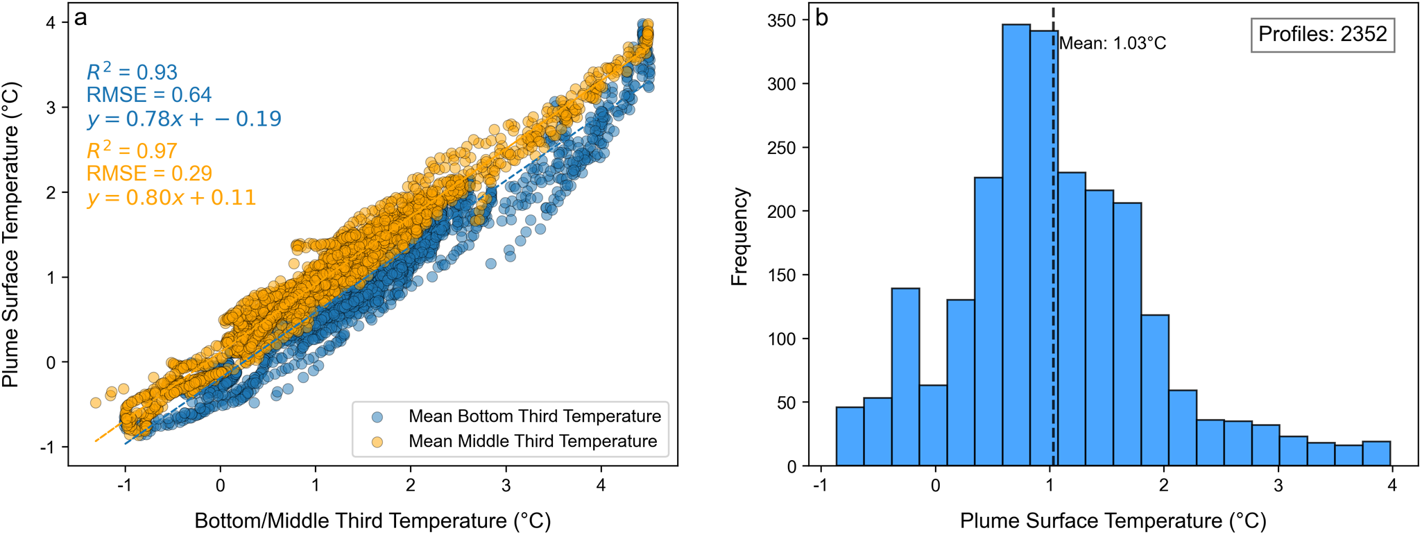
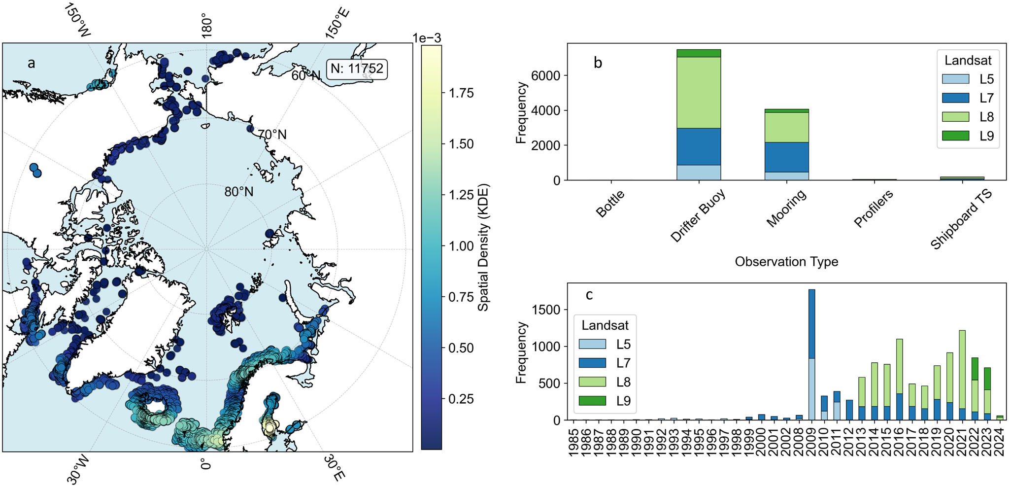
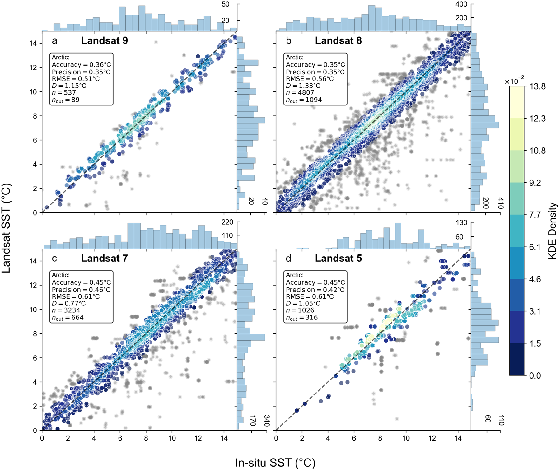
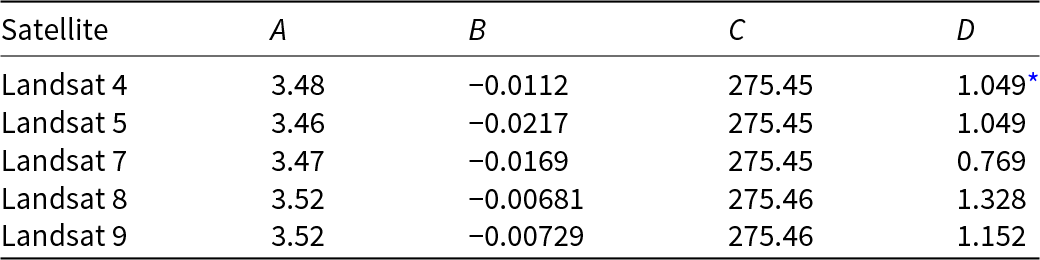
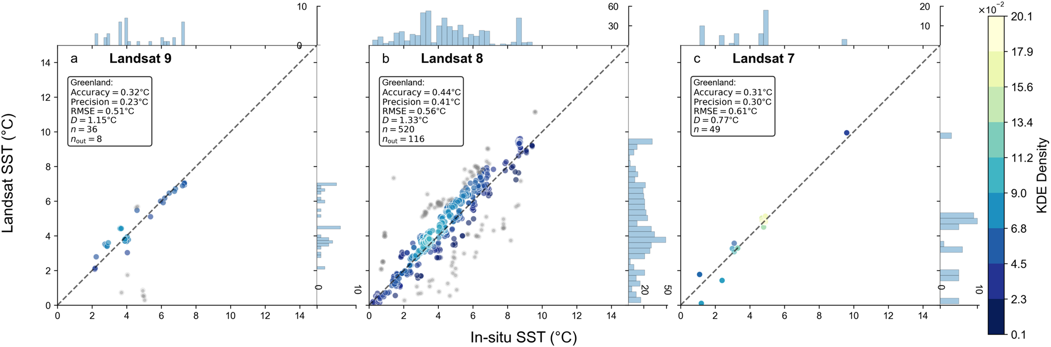
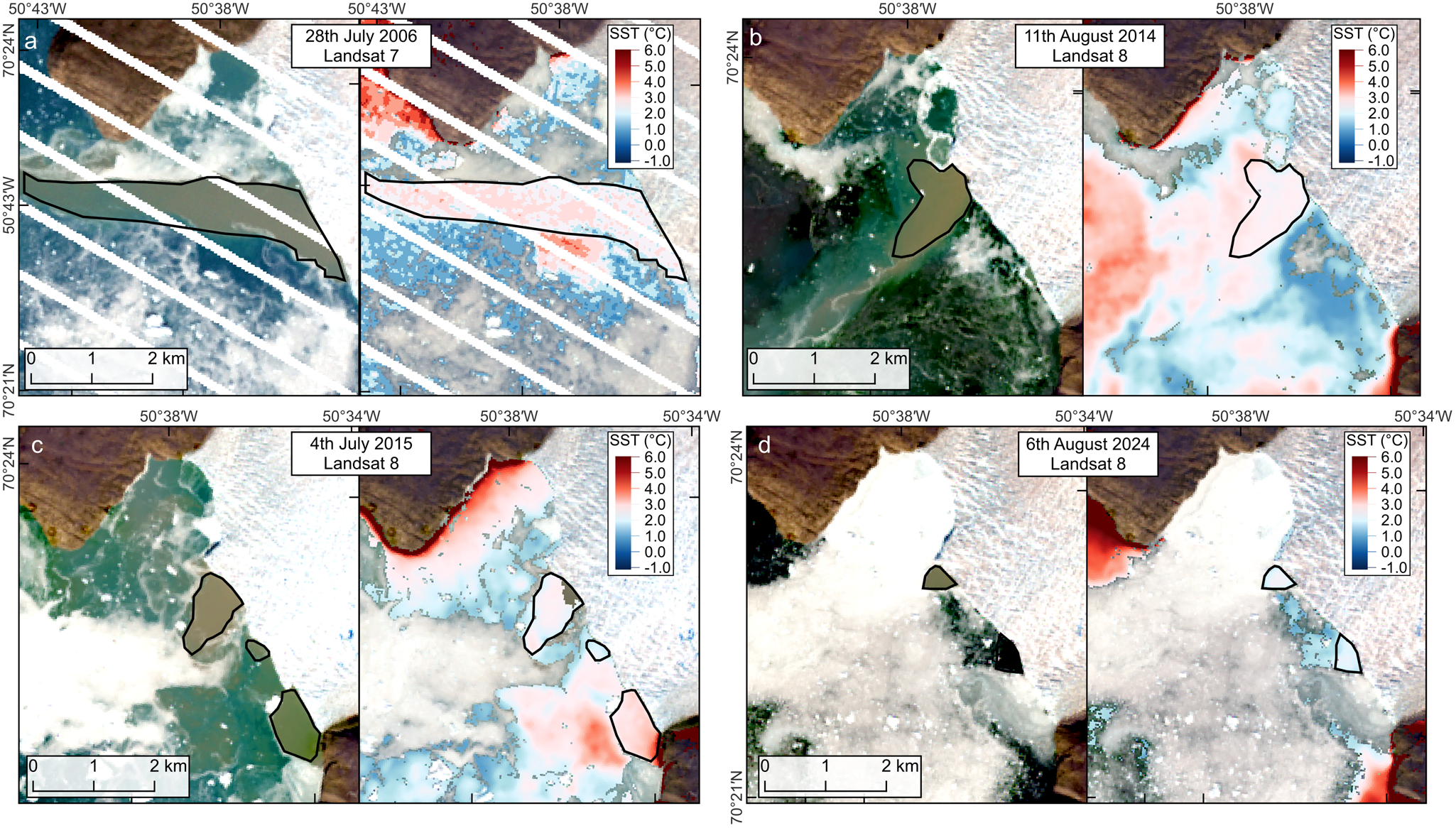
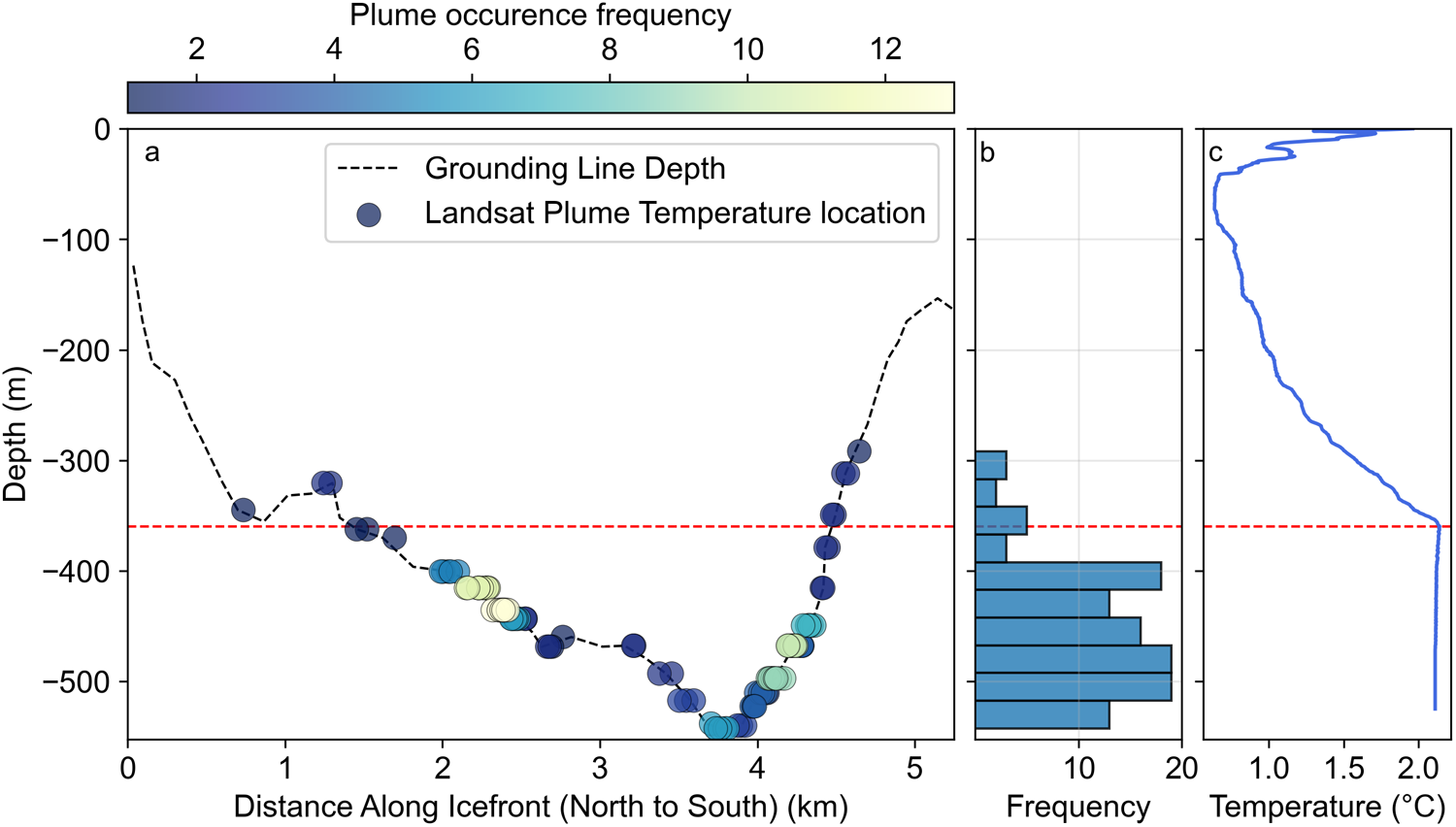
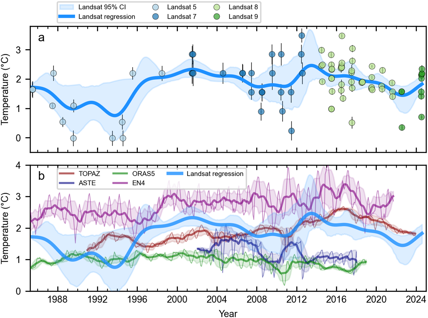


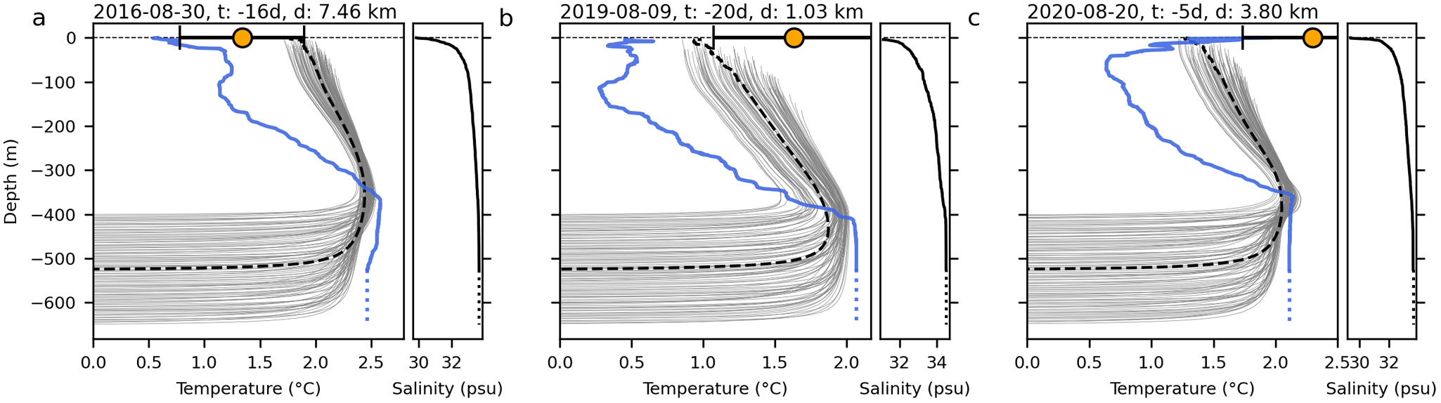


 Open access

