Introduction
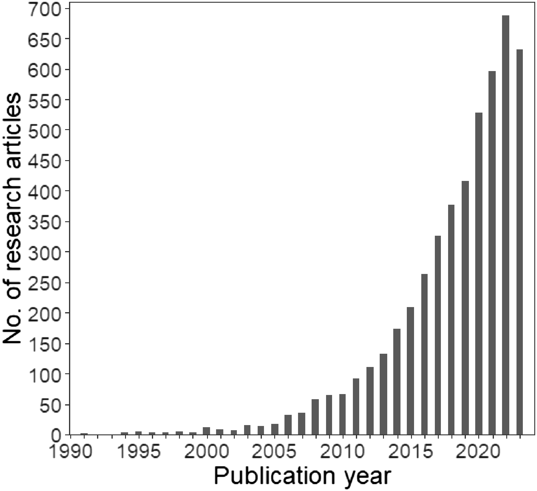
Since the 2000s, the realm of wildlife monitoring has entered a new era marked by the emergence of a wide variety of cutting-edge digital technologies (Berger-Tal and Lahoz-Monfort Reference Berger-Tal and Lahoz-Monfort2018; Schulz et al. Reference Schulz, Shriver, Stathatos, Seleb, Weigel, Chang, Saad Bhamla, Hu and Mendelson2023). The use of camera traps has grown exponentially, particularly over the last decade, with a considerable increase of 374% in the number of studies referring to this technology (Figure 1). The objectives of camera-trap studies include modelling presence-absence, relative abundance, occupancy, and/or density of single or multiple species (Burton et al. Reference Burton, Neilson, Moreira, Ladle, Steenweg, Fisher, Bayne and Boutin2015), which provide invaluable data for addressing conservation challenges and guiding wildlife management (Schulz et al. Reference Schulz, Shriver, Stathatos, Seleb, Weigel, Chang, Saad Bhamla, Hu and Mendelson2023). Although camera traps have undoubtedly improved efficiency in biodiversity assessment (Wearn and Glover-Kapfer Reference Wearn and Glover-Kapfer2019), questions remain about the ecological processes underlying species detection and how multiple detections of unmarked individuals affect the reliability of population abundance or density estimates (Gilbert et al. Reference Gilbert, Clare, Stenglein and Zuckerberg2021).
Number of research articles related to camera traps published over years. This figure updates the results of Burton et al. (Reference Burton, Neilson, Moreira, Ladle, Steenweg, Fisher, Bayne and Boutin2015) and Gilbert et al. (Reference Gilbert, Clare, Stenglein and Zuckerberg2021), using the same search terms in Web of Science: (camera trap* OR remote camera*) AND (wildlife OR mammal* OR bird*). The search was completed on 25 April 2024 and returned 5132 research articles published from 1991 to 2023.

Several modelling procedures exist for analysing camera-trap data. From the 359 studies reviewed by Burton et al. (Reference Burton, Neilson, Moreira, Ladle, Steenweg, Fisher, Bayne and Boutin2015), 41.4% used presence-absence and 43.6% relied on relative abundance indices as response variables, with neither procedure controlling for variation in detection. Occurrence models are often used because they ensure data independence by disregarding repeated captures (i.e., photographs) of unmarked individuals of the same species per occasion and site. However, these models may ignore spatial ecological processes influenced by density-dependent effects that shape the animal distribution in heterogeneous environments. These include animal movements (Broadley et al. Reference Broadley, Burton, Avgar and Boutin2019), habitat selection (van Beest et al. Reference van Beest, McLoughlin, Mysterud and Brook2016), competition for resources (Fretwell and Lucas Reference Fretwell and Lucas1970), predator-prey interactions (Sand et al. Reference Sand, Eklund, Zimmermann, Wikenros and Wabakken2016), or dispersal in metapopulation functioning (Andreassen and Ims Reference Andreassen and Ims2001). Although a positive abundance–occupancy relationship has been widely documented across taxa (Freckleton et al. Reference Freckleton, Noble and Webb2006; Gaston et al. Reference Gaston, Blackburn, Greenwood, Gregory, Quinn and Lawton2000)–particularly in vertebrates (de la Fuente et al. Reference de la Fuente, Hirsch, Cernusak and Williams2021; Weber et al. Reference Weber, Stevens, Diniz-Filho and Grelle2017), including mammals (Wen et al. Reference Wen, Cheng, Ge, Xia, Lv and Yang2018)–recent studies have reported that occurrence models may fail to characterise the environmental drivers and distribution of population abundance (e.g., in reptiles: Dibner et al. Reference Dibner, Doak and Murphy2017; birds: Estrada and Arroyo Reference Estrada and Arroyo2012; arthropods: Jiménez-Valverde et al. Reference Jiménez-Valverde, Diniz, Azevedo and Borges2009). Consequently, occurrence models might be less effective in capturing and understanding mechanisms driving population decline, which raises concerns for conservation purposes.
Abundance models are used as alternatives to occurrence modelling. Indeed, the camera-trap rate (i.e., number of photographs of a species divided by the number of trap-days per site; Bowkett et al. Reference Bowkett, Rovero and Marshall2008) is highly correlated with abundance in mammals (see Rovero and Marshall Reference Rovero and Marshall2009 for Harvey’s duiker) and has therefore been commonly used as a proxy for abundance of individuals (Martin-Garcia et al. Reference Martin-Garcia, Rodríguez-Recio, Peragón, Bueno and Virgós2022). Because multiple counts of the same individual may inflate the abundance estimates, most studies apply a time-to-independence threshold, defined as the elapsed time between consecutive photographs used to define independent detection events (Burton et al. Reference Burton, Neilson, Moreira, Ladle, Steenweg, Fisher, Bayne and Boutin2015). For instance, of the 134 camera-trap studies reviewed by Peral et al. (Reference Peral, Landman and Kerley2022), 32% applied no time-to-independence thresholds (i.e., all photographs are conserved, e.g., Dykstra et al. Reference Dykstra, Baruzzi, VerCauteren, Strickland and Lashley2023), 30% used a 30-min threshold (i.e., for a given species at a given camera trap, only photographs taken at least 30 min apart are considered independent), 21% used a 60-min threshold, and 5% a 24-hour threshold (see also Burton et al. Reference Burton, Neilson, Moreira, Ladle, Steenweg, Fisher, Bayne and Boutin2015). While ensuring data independence is required to comply with the assumption of abundance modelling (Goldstein et al. Reference Goldstein, Jensen, Kays, Cove, McShea, Rooney, Kierepka and Pacifici2024), the consequences of the choice of user-defined thresholds on results remain to be quantified (but see Peral et al. Reference Peral, Landman and Kerley2022).
Animal detection varies with local environmental conditions (e.g., vegetation openness; Amiot et al. Reference Amiot, Santos, Arvor, Bellón, Fritz, Harmange, Holland, Melo, Metzger, Renaud, Roque, Souza and Pays2021) or technical characteristics of the camera trap (e.g., sensor sensitivity; Driessen et al. Reference Driessen, Jarman, Troy and Callander2017). Ignoring imperfect detection can confound ecological processes with observational biases, potentially resulting in underestimating species occupancy or abundance when detection probability is less than 1 (Burton et al. Reference Burton, Neilson, Moreira, Ladle, Steenweg, Fisher, Bayne and Boutin2015) or overestimating them if repeated captures of the same individual are not properly addressed. Consequently, recent analytical advances have been developed as hierarchical processes that first estimate variation in detection before testing the influence of environmental predictors on animal occurrence or relative abundance (Kellner et al. Reference Kellner, Smith, Royle, Kéry, Belant and Chandler2023). Specifically, occupancy and N-mixture models have gained popularity with the development of the R package unmarked (Fiske and Chandler Reference Fiske and Chandler2011), establishing them as the most widely used hierarchical modelling approaches for studying the occurrence and relative abundance of unmarked animal populations (Rozylowicz et al. Reference Rozylowicz, Popescu, Manolache, Nita, Gradinaru, Mirea and Bancila2024). Faced with the diversity of approaches used for camera-trap data analyses, quantifying how commonly used modelling procedures (i.e., based on occurrence vs abundance data), their capacity to control for imperfect detection, and their implementation (e.g., application of time-to-independence thresholds) may affect our ability to capture ecological responses and spatially predict species distribution is key to prevent misallocation of resources and misplaced conservation efforts.
The current study aimed to examine (1) how commonly used species distribution modelling procedures, detection, and implementation can affect the ability to capture effects of environmental variables on animal occurrence or relative abundance, and (2) how these modelling procedures affect predicted species distribution maps. It is worth noting that the current study does not aim to provide a systematic review or to address all methodological issues related to camera-trap data analysis (see Burton et al. Reference Burton, Neilson, Moreira, Ladle, Steenweg, Fisher, Bayne and Boutin2015; Gilbert et al. Reference Gilbert, Clare, Stenglein and Zuckerberg2021; Rozylowicz et al. Reference Rozylowicz, Popescu, Manolache, Nita, Gradinaru, Mirea and Bancila2024; and Tanwar et al. Reference Tanwar, Sadhu and Jhala2021 for that purpose), nor to develop a comprehensive species distribution model for the study species. Rather, building on modelling procedures and species responses previously documented in the literature, this methodological study aims to evaluate how different, commonly used statistical procedures may affect the detection of key environmental effects (i.e., mean patch area of savanna and proportion of land burned) on the tapeti Sylvilagus brasiliensis sensu lato (Cordeiro-Estrela Reference Cordeiro-Estrela2022) and its predicted distribution.
The tapeti was monitored using camera traps in the Kadiwéu indigenous territory, located at the Cerrado-Pantanal ecotone (Mato Grosso do Sul, Brazil). This region is primarily composed of a mosaic of savanna, deciduous seasonal forests, and periodically flooded grasslands. Based on the established positive relationship between abundance and occupancy (Freckleton et al. Reference Freckleton, Noble and Webb2006), we first expected the environmental predictors, including fire and land-cover variables, would influence species occurrence and abundance (but see Parsons et al. Reference Parsons, Forrester, McShea, Baker-Whatton, Millspaugh and Kays2017). Secondly, we expected that variation in detection, potentially affected by factors such as vegetation openness or camera-trap model, could influence the estimates of environmental effects and the predicted species distributions if not properly addressed using hierarchical models. Specifically, because reduced vegetation openness is expected to impair detection, not accounting for it in the models might lead to underestimation–or even failure to detect–a positive relationship between native vegetation and tapeti presence and/or abundance. Thirdly, the application of time-to-independence thresholds in abundance modelling to ensure data independence should reduce double counting of individuals and effect overestimation, although it could also significantly reduce the number of animal captures available for analysis (Lepard et al. Reference Lepard, Moll, Cepek, Lorch, Dennis, Robison and Montgomery2018), potentially limiting the ability to detect environmental effects.
Material and methods
Study area
The Kadiwéu Indigenous Territory (from 20°10′45.59″ to 21°03′10.55″ S and from 56°50′52.30″to 57°50′51.27″W), located in Mato Grosso do Sul, Brazil, spans 5,400 km2 in a transition zone between two biomes: the Pantanal wetland and the Cerrado savanna (Oliveira et al. Reference Oliveira, Ferreira, Souza, Lopes, Bolzan, Roque, Pott, Pereira, Garcia, Damasceno, Costa, Rocha, Xavier, Ferraz and Ribeiro2022) (Figure 2a). Elevation follows a west–east gradient, ranging from 69 m in the Pantanal floodplain (west) to 819 m on the Bodoquena Plateau (east). Mean annual temperatures ranged from 25.2°C to 28.7°C (average = 26.4°C) over the period 2001–2018, and annual rainfall ranged from 360 mm to 1,000 mm (average = 660 mm) (Oliveira et al. Reference Oliveira, Ferreira, Souza, Lopes, Bolzan, Roque, Pott, Pereira, Garcia, Damasceno, Costa, Rocha, Xavier, Ferraz and Ribeiro2022). The vegetation is primarily characterised by savanna, deciduous seasonal forests, and periodically flooded grasslands (Ferreira et al. Reference Ferreira, Guerra, da Rosa Oliveira, Reis, Aptroot, Ribeiro and Garcia2021; Silva et al. Reference Silva, Silva and Mauro2014) (Figure 2b). In both the Cerrado and Pantanal, fires are recurrent, annually burning areas of several tens of thousands of square kilometres (Araújo et al. Reference Araújo, Ferreira and Arantes2012; Libonati et al. Reference Libonati, DaCamara, Peres, Sander de Carvalho and Garcia2020).
Location (a) and land-cover characterisation (b) of the Kadiwéu Indigenous Territory in the State of Mato Grosso do Sul, Brazil. Land cover at camera-trap sites (n = 36) is shown in panel (c). The land-cover classification was produced and published by Harmange et al. (Reference Harmange, Teles, Ribeiro, Costa, Godoi, de Oliveira Roque, Souza and Pays2024), derived from the 2021 MapBiomas land-cover map (7th collection). See Appendix A for details.

Camera-trap data
We used a camera-trap dataset collected from 24 June to 24 August 2021 in the eastern part of the Kadiwéu Indigenous Territory (Figure 2b–c), as published in Harmange et al. (Reference Harmange, Teles, Ribeiro, Costa, Godoi, de Oliveira Roque, Souza and Pays2024). This allowed sampling to be concentrated within a single season (winter), thereby ensuring homogeneous environmental conditions across all sites. 36 sites were monitored using camera traps (Bushnell Trophy Cam Aggressor Brown and Reconyx Hyperfire HC 500) for 30 consecutive days–ensuring homogeneous environmental conditions within each site–either from 24 June to 24 July (n = 15) or from 25 July to 24 August (n = 21). This resulted in a total of 1,080 camera-trap days, with all sites subjected to the same sampling effort. The delay-period setting–defined as the interval between consecutive photographs (Lepard et al. Reference Lepard, Moll, Cepek, Lorch, Dennis, Robison and Montgomery2018)–was set to 3 seconds. This 3-second delay was chosen to maximise data collection while preventing memory overload, which could have interrupted monitoring before the full one-month session was completed. Photographs were downloaded and analysed visually using Wild.ID (http://www.wildlifeinsights.org/team-network). Here, we specifically examined camera-trap data of the tapeti Sylvilagus brasiliensis sensu lato.
Environmental variables
Land cover
To characterise the land cover at camera-trap locations, we used the land-cover classification map produced by Harmange et al. (Reference Harmange, Teles, Ribeiro, Costa, Godoi, de Oliveira Roque, Souza and Pays2024), which was based on the 2021 MapBiomas land-cover map (7th collection) (Souza et al., 2020), derived from Landsat images (30-m resolution) (see Figure 2b and Appendix A for details).
In the current study, we examined the effect of land cover on the tapeti, focusing specifically on the mean patch area of savanna, which was previously identified as the unique land-cover variable affecting the distribution of the study species, among a set of seven variables, including the proportion and the mean patch area of the three main land-cover types (i.e., savanna, forest and grassland), as well as the density of edges between these land-cover types (Harmange et al. Reference Harmange, Teles, Ribeiro, Costa, Godoi, de Oliveira Roque, Souza and Pays2024). This variable was calculated using the R package landscapemetrics (Hesselbarth et al. Reference Hesselbarth, Sciaini, With, Wiegand and Nowosad2019) within buffers with a 500-m radius from each camera-trap location. This buffer extent was previously found to best predict the response of the studied species to both land cover and fire (Harmange et al. Reference Harmange, Teles, Ribeiro, Costa, Godoi, de Oliveira Roque, Souza and Pays2024).
Fire regime
To characterise the fire regime at camera-trap locations, we used the 2021 MapBiomas Fire products (2nd collection), derived from Landsat images (30-m resolution). We specifically focused on the proportion of land burned within the 12 months preceding monitoring, as this variable was previously identified as the only fire-related variable affecting the distribution of the tapeti among a set of five variables, including the mean and maximum fire frequency recorded over the period 1985–2021, the proportion of land burned twice during the twelve months preceding the monitoring, and the time since fire (Harmange et al. Reference Harmange, Teles, Ribeiro, Costa, Godoi, de Oliveira Roque, Souza and Pays2024; see also Júnior et al. Reference Júnior, Oliveira, Dias and Oliveira2005; Deus et al. Reference Deus, Burs, Fieker, Tissiani, Marques and Schuchmann2023).
The proportion of land burned within the 12 months preceding the monitoring was calculated, at each camera-trap location, as the proportion of pixels within a 500-m radius buffer that burned during the 12 months prior to the monitoring. This variable was based on the MapBiomas Fire product ‘Monthly burned coverage’ for the years 2020 and 2021.
This variable was weakly correlated with the mean patch area of savanna (Pearson’s correlation: r = −0.33; p = 0.046), remaining below the commonly accepted threshold of 0.7 for considering variables as uncorrelated in species distribution models (Barbet-Massin and Jetz Reference Barbet-Massin and Jetz2014; Leroy et al. Reference Leroy, Paschetta, Canard, Bakkenes, Isaia and Ysnel2013), and also below the more restrictive threshold of 0.5 occasionally applied in the literature (Renner et al. Reference Renner, Louvrier and Gimenez2019).
Preparation of environmental variables for species distribution mapping
The two environmental variables were calculated across the entire study area to extrapolate species distribution from model predictions and compare distribution maps predicted from the different modelling procedures (see Section “Comparison of the predicted species distribution maps”). We divided the Kadiwéu IT into a grid of 1000-m-wide hexagonal cells (n = 5935). Hexagons have the advantage of having a geometry close to the circular buffers while ensuring that there are no gaps or overlaps between neighbouring cells (see also Jurasinski and Beierkuhnlein Reference Jurasinski and Beierkuhnlein2006; Koetke et al. Reference Koetke, Hodder and Johnson2024). The 1000-m width of the hexagons was chosen to align with the scale (i.e., 500-m radius or 1000-m diameter) used to calculate the variables used in the models. The two environmental variables were then calculated within each hexagonal cell following the process described above.
Statistical analyses
We ran two commonly used approaches for occurrence and abundance modelling (Table 1) (Martin-Garcia et al. Reference Martin-Garcia, Rodríguez-Recio, Peragón, Bueno and Virgós2022). Firstly, we used generalised linear models (GLMs) on occurrence and abundance data. Secondly, we applied hierarchical modelling procedures: occupancy models for occurrence data and N-mixture models for abundance data. We used the number of photographs as a proxy for tapeti relative abundance, as is common for unmarked terrestrial mammals when individual recognition is not feasible (see Bowkett et al. Reference Bowkett, Rovero and Marshall2008; Martin-Garcia et al. Reference Martin-Garcia, Rodríguez-Recio, Peragón, Bueno and Virgós2022; Rovero and Marshall Reference Rovero and Marshall2009). We used the raw number of photographs of the study species rather than the camera-trap rate (i.e., number of photographs per species divided by the number of camera-trap days), as sampling effort was consistent across all sites. To ensure consistency in the comparison of GLMs and hierarchical modelling procedures, two camera traps were not considered in the statistical analyses due to missing detection information (i.e., visibility and camera-trap model; see Section “Hierarchical models”).
Summary of the modelling procedures

Generalized linear models (GLMs)
Although they do not control for imperfect detection, GLMs have commonly been used as a simple procedure in modelling the occurrence (e.g., Villaseñor et al. Reference Villaseñor, Blanchard, Driscoll, Gibbons and Lindenmayer2015) or relative abundance (e.g., Bowkett et al. Reference Bowkett, Rovero and Marshall2008; Piña et al. Reference Piña, Carvalho, Rosalino and Hilário2019; Rocha et al. Reference Rocha, Ramalho and Magnusson2016) of vertebrates from camera-trap data.
Firstly, we used a GLM (binomial, logit link) to model the probability of occurrence of the model species as a function of the two environmental variables previously described. For each camera trap location, we assigned the value 1 when the species was detected at least once during the monitoring and 0 when it was not. This variable was used as the dependent variable in models. All candidate models, ranging from a full model (including the two independent variables and their interaction) to a null (intercept-only) model, were considered in the model selection. Models were selected based on Akaike’s information criterion (Burnham and Anderson Reference Burnham and Anderson2002). We selected the final model based on (1) the lowest AIC value (i.e., the strongest statistical support) and (2) a difference in AIC (ΔAIC) > 2 with the null model. Competing models with a difference in AIC (ΔAIC) < 2 were considered with equivalent statistical support.
Similarly, we modelled the relationship between the relative abundance of the species and the environmental variables using a GLM (Poisson, log link). Because multiple counts of the same individual compromise the condition of data independence, analyses were replicated using the most common time-to-independence thresholds (Burton et al. Reference Burton, Neilson, Moreira, Ladle, Steenweg, Fisher, Bayne and Boutin2015; Peral et al. Reference Peral, Landman and Kerley2022): no threshold, or thresholds of 30 min (i.e., for a given species at a given camera trap, only photographs taken at least 30 min apart are considered), 60 min and 24 hours. All candidate models, ranging from a full model (including the two independent variables and their interaction) to a null model, were considered. For each of the tested thresholds, the best candidate models were selected based on Akaike’s information criterion following the process described above.
Hierarchical models
Hierarchical models account for imperfect detection by estimating detection probabilities from repeated observations across sampling occasions. For each camera-trap location, we built a matrix of 5 sampling occasions, each consisting of 6 consecutive days (see also Ribeiro et al. Reference Ribeiro, Nichols, Morato, Metzger and Pardini2019; Amiot et al. Reference Amiot, Santos, Arvor, Bellón, Fritz, Harmange, Holland, Melo, Metzger, Renaud, Roque, Souza and Pays2021).
Firstly, for occurrence data, we assigned the value 1 to a camera-trap location, at a given occasion, when the model species was captured, and 0 when it was not. We then used occupancy models (Table 1). The occupancy probability (ψ) of the model species at each camera-trap location and the detection probability (pd) were modelled as a function of the environmental (xi) and detection (zi) variables using logit link functions.
The detection probability (pd) was estimated using a stepwise process starting with the ‘null model’ ψ(.)pd(.), where the occupancy and detection probabilities are constant. The probability of an individual being captured at the sampling site can be influenced by several factors. These include visibility, which depends on the vegetation openness in front of the camera trap (potentially–though unlikely–influenced by seasonality during the study period), and/or the technical characteristics of the camera-trap model (e.g., sensor sensitivity). We computed two detection variables zi: visibility (open vs. dense vegetation) and camera-trap model (Bushnell® and RECONYX®). The effect of detection variables was estimated by running three models ψ(.)pd(zi), to test whether the zi variables including visibility, camera-trap model, or both, affected the detection probability (pd), when the occupancy (ψ) was constant. These three models and the null model were compared using Akaike’s Information Criterion (AIC) (Burnham and Anderson Reference Burnham and Anderson2002). We selected as the ‘null detection model’ the model with the lowest AIC value and a difference in AIC (ΔAIC) > 2 with the null model.
We then tested the effect of the environmental variables on the occupancy (ψ) of the model species. Five models were run and compared using AIC: the model incorporating the interaction between fire and land cover ψ(fire*land cover) pd(zi), the model with the additive effect of fire and land cover ψ(fire+land cover) pd(zi), the two univariate models ψ(fire) pd(zi) and ψ(land cover) pd(zi), and the null detection model. We selected the final model based on the lowest AIC value and a difference in AIC (ΔAIC) > 2 with the null detection model.
Secondly, for abundance data, we assigned into the matrix the number of photographs per camera trap per occasion, which is commonly used as a proxy for relative abundance (see Martin-Garcia et al. Reference Martin-Garcia, Rodríguez-Recio, Peragón, Bueno and Virgós2022). As with GLMs, multiple photographs of the same individual can compromise data independence and bias relative abundance estimates. Therefore, abundance analyses were repeated using the most common time-to-independence thresholds (i.e., no threshold, 30 min, 60 min, and 24 hours) to filter out the data prior to preparing the matrix. We then used N-mixture models (Table 1) (Royle Reference Royle2004). In the literature, two common approaches are used for fitting N-mixture models to camera-trap data: (1) using the number of photographs captured during each sampling occasion as a proxy for relative abundance (e.g., Martin-Garcia et al. Reference Martin-Garcia, Rodríguez-Recio, Peragón, Bueno and Virgós2022); and (2) summing the maximal number of individuals captured in each photograph during each sampling occasion (e.g., Harris et al. Reference Harris, Stewart, Butler, Rominger, Ruhl, McDonald and Schmidt2024). In our study, since the maximum number of tapeti captured in a single photograph was 1, our modelling procedure aligns with both of these approaches. The relative abundance (λ), approximated using the number of photographs of the species captured by the camera traps aggregated into 6-day occasions, and the detection probability (pd) were modelled as a function of the environmental (xi) and detection (zi) variables using log and logit link functions, respectively. The modelling process applied was rigorously the same as for occupancy models.
The detection probability (pd) was estimated starting with the ‘null model’ λ(.)pd(.), where the relative abundance and detection probabilities are constant. The effect of detection variables was estimated by running three models, λ(.)pd(zi), to test whether the zi variables, including visibility, camera-trap model, or both, affected the detection probability (pd) when the relative abundance (λ) was constant. Models were compared using AIC to select the ‘null detection model’.
We finally tested the effect of environmental variables on the relative abundance (λ) of the model species by comparing five models using AIC: the model incorporating the interaction between fire and land cover λ(fire*land cover) pd(zi), the model with the additive effect of fire and land cover λ(fire+land cover) pd(zi), the two univariate models λ(fire) pd(zi) and λ(land cover) pd(zi), and the null detection model.
Comparison of the predicted species distribution maps
Predicted distribution maps of the species were prepared for each of the modelling procedures. The predicted probability of occurrence, or relative abundance, of the species was calculated from the selected models using the R-function predict, based on the variables previously calculated within hexagonal cells as environmental predictors (see Section “Preparation of environmental variables for species distribution mapping”).
For each map, the predicted value of each hexagonal cell was divided by the sum of all predicted values (i.e., values of all hexagons) across the Kadiwéu IT. This ensures that the sum of standardised values across all hexagons equals 1, providing a common scale for comparing species distribution maps.
We then conducted pairwise comparisons between the standardised maps predicted from the different modelling procedures using two statistics. Firstly, to assess the convergence of species distributions, we calculated Pearson’s correlation coefficient for the standardised values of the compared maps.
Secondly, pinpointing the areas where a focal species is most likely to occur, or where it is predicted to be most abundant in a study area, is critical for informing the effective delineation of priority areas for management or conservation planning. Standardised maps were thus transformed into binary maps distinguishing areas of high versus moderate-to-low predicted probability of occurrence or relative abundance of the species. For each map, we assigned the value 1 to hexagonal cells with predicted values greater than or equal to the 9th quantile of standardised values across all hexagons and 0 to cells with standardised values below this threshold. This threshold ensures that the hexagons with the 10% highest predicted values of probability of occurrence or relative abundance are identified as the most relevant for delineating (simulated) priority areas. We calculated the Cohen’s Kappa statistic to compare the binary maps (Allouche et al. Reference Allouche, Tsoar and Kadmon2006; Manel et al. Reference Manel, Williams and Ormerod2001). The Kappa statistic measures the agreement between two categorical maps and accounts for both commission and omission errors in a single statistic (Allouche et al. Reference Allouche, Tsoar and Kadmon2006; Manel et al. Reference Manel, Williams and Ormerod2001). Kappa’s coefficient ranges from −1 to 1, with levels of agreement interpreted as poor (Kappa ≤ 0), fair (0–0.20), moderate (0.20–0.45), substantial (0.45–0.75), almost perfect (0.75–1), and perfect (Kappa = 1) (Munoz and Bangdiwala Reference Munoz and Bangdiwala1997).
All data preparation and analyses were performed using R software (R Core Team 2022).
Results
The tapeti Sylvilagus brasiliensis sensu lato was detected in 8 (22%) of the 36 camera-trap locations, resulting in 183 captures. Applying a time-to-independence threshold to avoid repeated counts of the same individuals in abundance analyses reduced the dataset by 86% to reach 25 captures for both the 30-min and 60-min thresholds (hereafter ‘30/60-min threshold’) and to 23 captures (−87%) for the 24-hour threshold.
Detected ecological responses
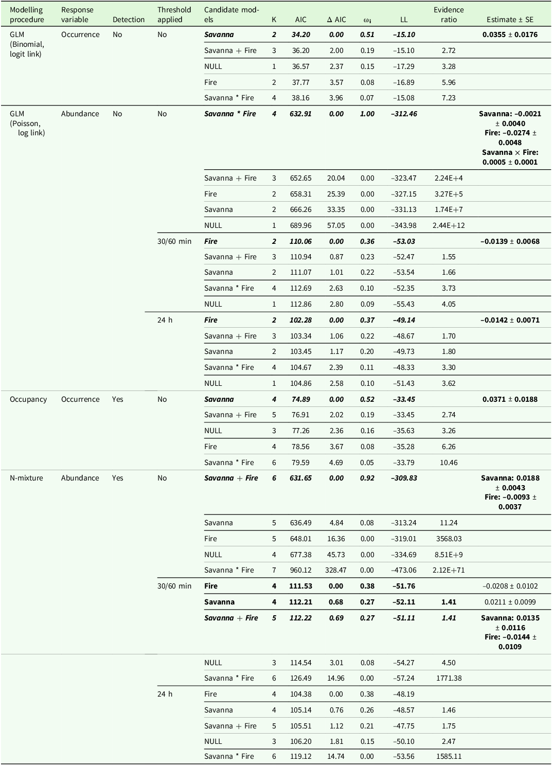
The two occurrence modelling procedures–whether controlling for imperfect detection (occupancy model) or not (GLM)–provided similar results (Table 2). Both detected that the tapeti occurrence increased with the mean patch area of savanna.
Statistical supports of models testing the univariate, additive, and interactive effects of land cover and fire variables on the occurrence or relative abundance of the model species, the tapeti Sylvilagus brasiliensis sensu lato, using four different modelling procedures (see Methods). GLMs do not control for imperfect detection, whereas hierarchical modelling procedures (i.e., occupancy and N-mixture abundance models) do. Abundance analyses were repeated using no time-to-independence threshold between consecutive photographs, 30/60-min, or 24-hour thresholds. The number of parameters (K), model weights (ωi), log likelihood values (LL), and AIC values are indicated. ΔAIC indicates the difference in AIC between the candidate model and the model with the lowest AIC value. Candidate models were considered significant when their AIC value was lower than the AIC of the null detection model (NULL), with an AIC difference (ΔAIC) > 2. All significant models with a ΔAIC < 2 from the model with the lowest AIC value had similar statistical supports and are indicated in bold. In this case, and when possible (i.e., if models were nested), the parsimony principle was applied to select the simplest model. The final selected models are represented in italics. Estimates ± SE are indicated for significant effects

Abundance models (based on the number of photographs as a proxy for relative abundance)–whether controlling (N-mixture models) or not (GLMs) for imperfect detection–detected effects of land cover and fire on the relative abundance of the tapeti (Table 2). Although the type of effects (i.e., univariate, additive or interactive) varied with the procedure and time-to-independence thresholds applied, the significant effects of environmental variables remained consistent between models: the relative abundance increased with the mean patch area of savanna and decreased with the proportion of land burned in the 12 months preceding monitoring (Table 2).
Results obtained from GLMs varied depending on whether a time-to-independence threshold was applied or not to filter out repeated captures of potentially the same individuals. When ignoring the issue of data independence (i.e., no threshold applied), the model detected an interactive effect between land cover and fire on the relative abundance of the species. However, this effect was no longer consistent when time-to-independence thresholds were applied. Regardless of the threshold used (i.e., either 30/60-min or 24-hour), the candidate model including fire as the unique predictor was the best model to predict the relative abundance of the species (Table 2).
Results from N-mixture models were more consistent, detecting additive effects of fire and land cover when data independence was ignored (no threshold) or not (thresholds of 30/60 min) (Table 2). In the latter case, the models including fire or land cover as the unique predictor, or the model including the additive effects of both variables received equivalent support (Table 2). The effects of fire or land cover were not detected when a 24-hour threshold was applied.
Predicted species distribution
While distribution maps predicted from occurrence data whether controlling or not for imperfect detection (Figure 3a, b) did not differ (correlation coefficient: r = 1.00, CI95% = 1.00–1.00; Figure 4a), maps predicted from abundance data greatly differed (Figure 3c–g). Specifically, the correlation coefficients between the maps produced from abundance models controlling (N-mixture models) or not (GLMs) for imperfect detection were moderate (Figure 4a), whether no threshold (r = 0.29, CI95% = 0.27–0.32) or a 30/60-min time-to-independence threshold (r = 0.53, CI95% = 0.51–0.55) was applied. Consequently, distribution maps predicted from N-mixture models were highly correlated with those derived from occurrence models whatever the time-to-independence threshold applied (no threshold: r = 0.90, CI95% = 0.90–0.91; 30/60 min: r = 0.74, CI95% = 0.73–0.75), whereas maps predicted from GLMs on abundance data were poorly correlated with those derived from occurrence models (no threshold: r = 0.34, CI95% = 0.31–0.36; 30/60 min: r = −0.11, CI95% = −0.13– −0.08; 24-hour: r = −0.11, CI95% = −0.13– −0.08) (Figure 4a). The two maps derived from the N-mixture models that ignored (no threshold) or accounted for (30/60-min threshold) data independence issues were similar (r = 0.95, CI95% = 0.95–0.96).
Maps of standardised predictions (see Methods) for the probability of occurrence (a, b) and relative abundance (c–g) of the model species, the tapeti Sylvilagus brasiliensis sensu lato, in the Kadiwéu Indigenous Territory, Mato Grosso do Sul, Brazil. Predictions come from generalised linear models that did not allow to control for imperfect detection (a, c, e, and g) or hierarchical models (b, d, and f) that did control for imperfect detection. Abundance analyses were repeated using no time-to-independence threshold between consecutive photographs (c, d), a 30/60-min threshold (e, f), or a 24-hour threshold (g).

(a) Matrix of Pearson’s correlation coefficients extracted from pairwise comparisons between standardised prediction maps of occurrence or relative abundance produced from all tested modelling procedures (see Figure 3). Modelling procedures are presented based on their ability to control for imperfect detection. (b) Matrix of Cohen’s Kappa obtained from pairwise comparisons between binary maps of high versus moderate probability of occurrence or relative abundance, produced from all tested modelling procedures (see Figure S1). The threshold used to distinguish between high and moderate values corresponds to the 9th quantile of predicted probability of occurrence or estimated relative abundance calculated across the entire study area (see Methods).

Binary maps simulate priority areas for conservation by pinpointing areas where the species is most likely to occur (Figure S1A, B in Appendix B) or where it is predicted to be most abundant (Figure S1C–G in Appendix B). Occurrence models, whether controlling for imperfect detection or not, provided rigorously identical priority maps (Kappa = 1.00; Figure 4b).
Priority maps predicted from GLMs on abundance data that did not account for imperfect detection were not consistent and showed only fair agreement (Kappa = 0.01; Figure 4b) between priority areas identified when ignoring (i.e., no time-to-independence threshold) or accounting for (i.e., 30/60-min or 24-hour threshold) data independence issues. Priority areas had moderate agreement with those identified by occurrence models when data independence issues were ignored (Kappa = 0.27; Figure 4b). However, they showed poor agreement (Kappa = −0.04; Figure 4b) when data independence was considered whatever the time-to-independence threshold used.
In contrast, when controlling for imperfect detection using N-mixture models, priority maps produced when ignoring (no threshold) or addressing (30/60 min threshold) data independence issues showed almost perfect agreement (Kappa = 0.93; Figure 4b). In both cases, priority areas identified from N-mixture models showed substantial agreement with those identified by occurrence models (no threshold: Kappa = 0.63; 30/60-min threshold: Kappa = 0.56; Figure 4b).
Discussion
Comparing occurrence versus abundance models
The number of significant environmental predictors detected was higher in modelling procedures based on abundance (using the number of photographs as a proxy for relative abundance) compared with occurrence data. Distribution maps predicted from occurrence and abundance N-mixture models that controlled for imperfect detection showed moderate discrepancies, while substantial differences were observed between maps predicted from occurrence models and abundance GLMs. A strong agreement between occurrence and relative abundance was expected due to the pervasive, positive abundance–occupancy relationship (Freckleton et al. Reference Freckleton, Noble and Webb2006; Gaston et al. Reference Gaston, Blackburn, Greenwood, Gregory, Quinn and Lawton2000). Indeed, effects of environmental variables on one of the two dimensions (i.e., occurrence or abundance) should have been expected to reverberate on the other.
The effects of environmental predictors detected by the modelling procedures differed between abundance and occurrence data. Dibner et al. (Reference Dibner, Doak and Murphy2017) showed that the effects detected using abundance models may vary in sign and magnitude compared with occupancy models. Our results further demonstrate that abundance models can detect additional ecological responses compared with occurrence models. Two explanations can be advanced. Firstly, the occurrence and abundance of the species may not be correlated. Jiménez-Valverde et al. (Reference Jiménez-Valverde, Diniz, Azevedo and Borges2009) found a weak correlation between occurrence and abundance for 48 arthropod species. Although similar patterns have been documented in some vertebrates (e.g., reptiles: Dibner et al. Reference Dibner, Doak and Murphy2017; birds: Estrada and Arroyo Reference Estrada and Arroyo2012), such findings remain rare and, to our knowledge, have not yet been reported in mammals. Secondly, because occurrence models do not account for the abundance of individuals, they may be less sensitive in capturing density-dependent effects. In our study, the effect of fire detected only from abundance models supports previous observations showing that vertebrate abundances may decline when the fire extent increases (Lawes et al. Reference Lawes, Murphy, Fisher, Woinarski, Edwards and Russell-Smith2015). Fire is also known to affect the number of visual observations and camera-trap detections in the tapeti (Deus et al. Reference Deus, Burs, Fieker, Tissiani, Marques and Schuchmann2023). However, this second hypothesis remains uncertain, as occurrence models were able to detect mean patch area effects, which have also been shown to affect the population density in birds, mammals, and insects (Bender et al. Reference Bender, Contreras and Fahrig1998). It should be noted that the study species was relatively scarce, being detected at 22% of camera-trap sites, and that the set of significant environmental variables was limited. While there is clear value in understanding how modelling procedures perform in capturing the ecological responses (even if limited) and in predicting the distributions of rare or elusive species, expanding this research to more abundant species–particularly herbivores–and incorporating a more comprehensive set of environmental variables, including local habitat conditions, would be highly valuable.
Further studies are needed to determine whether the discrepancies result from a real lack of correlation between occurrence and abundance data or from an analytical artefact. Additionally, while our approach aligns with commonly used methods for assessing relative abundance from camera-trap data of unmarked animal populations, further investigation is needed to evaluate the consequences of using the number of photographs captured (e.g., Martin-Garcia et al. Reference Martin-Garcia, Rodríguez-Recio, Peragón, Bueno and Virgós2022) versus the sum of the maximum number of individuals per photograph (e.g., Harris et al. Reference Harris, Stewart, Butler, Rominger, Ruhl, McDonald and Schmidt2024) when estimating population abundance.
Imperfect detection
Not accounting for imperfect detection had little influence on occurrence models. GLM detected the same environmental effects and produced a similar species distribution map as the occupancy model. This suggests that detection variables included in the model had a negligible effect on detecting the species. This might be explained by the use of a 6-day sampling occasion, which was likely long enough to detect the species under all tested conditions, i.e., regardless of vegetation openness or camera-trap model. While we cannot entirely exclude the possibility that additional factors (e.g., weather conditions) may have influenced detection, we consider this unlikely, as sampling was conducted within a single season (winter), ensuring homogeneous conditions across all sites. However, this result does not question the usefulness of accounting for imperfect detection, as our results are based on a single species and a limited set of environmental variables. Guillera-Arroita et al. (Reference Guillera-Arroita, Lahoz-Monfort, MacKenzie, Wintle and McCarthy2014) caution that ignoring imperfect detection in occupancy analyses can confound occupancy with detection and produce erroneous estimates contrasting markedly with true occupancy. Although more complex, occupancy models can detect the effects of environmental variables, even if the sampling effort is low (i.e., 36 camera traps). They should be systematically preferred as a safeguard to ensure the reliability and accuracy of occurrence estimates (Guillera-Arroita et al. Reference Guillera-Arroita, Lahoz-Monfort, MacKenzie, Wintle and McCarthy2014).
Accounting for imperfect detection appears even more relevant for abundance models. GLMs that ignored imperfect detection produced different results. The interactive effect identified between land cover and fire when ignoring data independence was not consistent when time-to-independence thresholds were applied. This does not necessarily imply that the results are incorrect but suggests they may be more susceptible to the decreasing resolution of data caused by the time-to-independence thresholds. In contrast, N-mixture models that controlled for imperfect detection consistently identified additive effects of land cover and fire, whether data independence was considered or not. This led to important discrepancies between the species distribution and priority maps predicted from GLMs and N-mixture models. Differences in the results obtained from the two procedures suggest that observational processes may be confounded with ecological processes in abundance GLMs. This aligns with Martin-Garcia et al. (Reference Martin-Garcia, Rodríguez-Recio, Peragón, Bueno and Virgós2022) who showed that GLMs misidentified predictors of red fox Vulpes vulpes detection as explanatory variables of abundance, thereby masking the effects of other relevant variables affecting fox abundance. They further found that N-mixture models provided reliable estimates of the environmental effects on fox abundance, including their sign and magnitude, comparable to those estimated from naturally marked, photo-identified individuals. Similarly, Keever et al. (Reference Keever, McGowan, Ditchkoff, Acker, Grand and Newbolt2017) found that N-mixture models were highly effective for producing accurate abundance estimates of marked white-tailed deer Odocoileus virginianus from camera-trap data. However, it is important to note that N-mixture models do not perform well in all situations (e.g., Koetke et al. Reference Koetke, Hodder and Johnson2024; Martijn et al. Reference Martijn, Jim, Natalie and Thomas2023; Nakashima Reference Nakashima2020), and assessing the accuracy of population abundance estimates remains essential.
In conclusion, while abundance GLMs can be used for analysing abundance of photo-identified individuals (Martin-Garcia et al. Reference Martin-Garcia, Rodríguez-Recio, Peragón, Bueno and Virgós2022), we strongly encourage the use of modelling procedures that control for imperfect detection when analysing camera-trap data of unmarked individuals.
Time-to-independence
Repeated captures of the same unmarked individuals may compromise data independence in abundance modelling. Although data independence issues should not be ignored as they affect model assumptions, Peral et al. (Reference Peral, Landman and Kerley2022) reported that 32% of the 134 reviewed camera-trap studies did not apply time-to-independence thresholds. Our study showed that, unlike GLMs, N-mixture models remained consistent in terms of the nature, sign, and magnitude of the detected environmental effects. The predicted species distribution and priority maps produced using this procedure also showed almost perfect agreement, whether or not data independence was considered. These results align with Lepard et al. (Reference Lepard, Moll, Cepek, Lorch, Dennis, Robison and Montgomery2018), who showed that a 60-min delay between consecutive photographs had a negligible impact on the results of hierarchical models.
Time-to-independence thresholds should be systematically applied as a safeguard to ensure model assumptions are met, thereby guaranteeing the reliability and accuracy of abundance estimates. Both 30-min and 60-min thresholds (not differentiable in our study), which are the most commonly applied (Burton et al. Reference Burton, Neilson, Moreira, Ladle, Steenweg, Fisher, Bayne and Boutin2015; Peral et al. Reference Peral, Landman and Kerley2022), provided equivalent results and proved to be effective in reducing repeated captures of unmarked individuals without affecting the ability to detect environmental effects.
Conservation implications and future directions
Quantifying biodiversity responses to environmental changes has become an urgent challenge. The use of camera traps and the availability of camera-trap databases (e.g., Lima et al. Reference Lima, Beca, Muylaert, Jenkins, Perilli, Paschoal, Massara, Paglia, Chiarello, Graipel, Cherem, Regolin, Oliveira Santos, Brocardo, Paviolo, Di Bitetti, Scoss, Rocha, Fusco-Costa, Rosa, Da Silva, Hufnagell, Santos, Duarte, Guimarães, Bailey, Rodrigues, Cunha, Fantacini, Batista, Bogoni, Tortato, Luiz, Peroni, De Castilho, Maccarini, Filho, Angelo, Cruz, Quiroga, Iezzi, Varela, Cavalcanti, Martensen, Maggiorini, Keesen, Nunes, Lessa, Cordeiro-Estrela, Beltrão, De Albuquerque, Ingberman, Cassano, Junior, Ribeiro and Galetti2017) provide invaluable resources to address this challenge. Our study reveals that the modelling procedure used to analyse camera-trap data is decisive for detecting environmental effects and producing species distribution maps.
Maps are critical tools used for decision-making in wildlife management and conservation (Lecours Reference Lecours2017). Inappropriate selection of modelling procedures could lead to misallocation of resources and conservation efforts, directed towards irrelevant priority areas. For analysing camera-trap data of unmarked individuals, we recommend: (1) the systematic use of hierarchical modelling controlling for imperfect detection (based on the methods evaluated in the current study, though alternative methods exist; e.g., Nakashima et al. Reference Nakashima, Fukasawa and Samejima2018), and (2) the application of a 30-min time-to-independence threshold in abundance models. These are essential safeguards to ensure that model assumptions are met and that biodiversity estimates are reliable, without compromising the ability to detect environmental effects.
Future research should focus on developing ecologically informed guidelines to accurately quantify ecological responses of biodiversity to environmental factors and to map species distribution from camera-trap data. Firstly, this includes disentangling occupancy and abundance (see also Dibner et al. Reference Dibner, Doak and Murphy2017) and quantifying the effectiveness of both modelling procedures in addressing density-dependent effects, to provide clear ecological arguments for choosing between occupancy or abundance models. Secondly, such guidelines should consider investigating the relationship between observational and ecological processes for population abundance estimates. Specifically, improving the accuracy of abundance estimates requires better estimates of the relationship between detection (i.e., the number of photographs) and actual abundance (i.e., the true number of individuals) in unmarked populations.
Further studies coupling camera-trapping with the monitoring of GPS-equipped or marked animals could successfully improve our understanding of how animal movements affect detection. Specifically, this approach would help quantify: (1) how intensive, area-concentrated search mode and exploitation of profitable places (Barraquand and Benhamou Reference Barraquand and Benhamou2008) inflates repeated captures of individuals per detection event per camera trap (Figure 5a), (2) how movement recursions to repeatedly visited areas (Riotte-Lambert et al. Reference Riotte-Lambert, Benhamou and Chamaillé-Jammes2013) increase the likelihood of detecting the same individual across multiple detection events within a camera trap–a particularly relevant issue for small-bodied, low-mobility species such as the tapeti (Figure 5b), and (3) how animal movement induces multiple detections of a single individual across neighbouring camera traps (Figure 5c; Broadley et al. Reference Broadley, Burton, Avgar and Boutin2019; Kays et al. Reference Kays, Hody, Jachowski and Parsons2021). Sociality may also increase the likelihood of detecting the same individuals (Figure 5d) if large groups reduce their movement and increase residence time (Pays et al. Reference Pays, Fortin, Gassani and Duchesne2012). Therefore, while applying a time-to-independence threshold appears relevant to ensure data independence, an inappropriate threshold could lead to underestimating the true abundance of individuals in social species.
Future challenges in improving abundance estimation of unmarked animal populations. Panels (a), (b), and (d) depict strategies to discriminate observational (i.e., detection) and ecological processes and to refine abundance estimates while ensuring data independence within a single camera trap. Panel (c) focuses on the challenge of maintaining data independence in the context of animal movement across multiple camera traps. Yellow-filled polygons indicate the camera trap field of view. The red-bounded polygons (Panels a and b) represent the home range of the animal. The red-shaded area (Panel a) denotes varying intensity of exploitation within the home range, with the clock icon symbolising the measure of residence time. Coloured bouts (Panel b) depict repeated movements (recursions) to the area in front of the camera trap over time. Blue arrows (Panels c and d) represent animal movement paths, highlighting the potential impact of movement on data independence across and within camera-trap locations. Credits: Tree and animal silhouettes were obtained freely from http://phylopic.org. The stone, clock, grass plot, and stripes were designed by Macrovector, Tohamina, and Freepik and are freely available on Freepik.

Supplementary material
The supplementary material for this article can be found at https://doi.org/10.1017/S0266467425100187
Acknowledgements
We thank the indigenous communities of the Kadiwéu reserve. We also thank Fabio O. Roque, Franco L. Souza, Letícia C. Garcia, Roland Kays, and Stefano Focardi for their valuable comments during the preliminary discussions of this work or the previous version of the manuscript.
Author contributions
Clément Harmange: conceptualisation, investigation, data curation, methodology, formal analysis, writing – original draft, writing – review & editing. Thiago Silva Teles: investigation, data curation, writing – review & editing. Danilo Bandini Ribeiro: funding acquisition, project administration, supervision, writing – review & editing. Anny M. Costa: investigation, data curation, writing – review & editing. Mauricio N. Godoi: investigation, data curation, writing – review & editing. Olivier Pays: funding acquisition, project administration, supervision, methodology, writing – review & editing.
Financial support
This study was funded by CNPQ [33/2018: 441948/2018-9], CAPES [23038.001818/2020-70; Capes-PrInt 41/2017: 88881.311897/2018-01] and COFECUB [Sv 875-17]. Additional funding support for OP, CH and TST was provided by the UA. TST was supported by a grant from CAPES-COFECUB [88887.647558/2021-00]. MNG received support from WWF-Brasil. DBR received support from Fundect [83/026.793/2024].
Competing interests
The author(s) declare none.