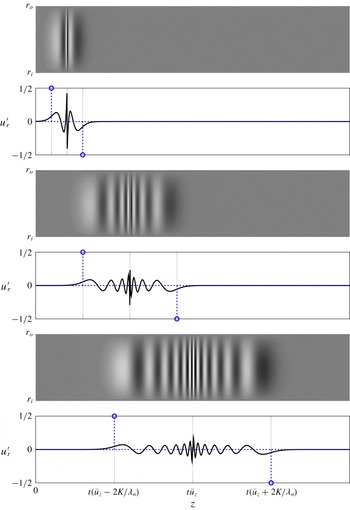
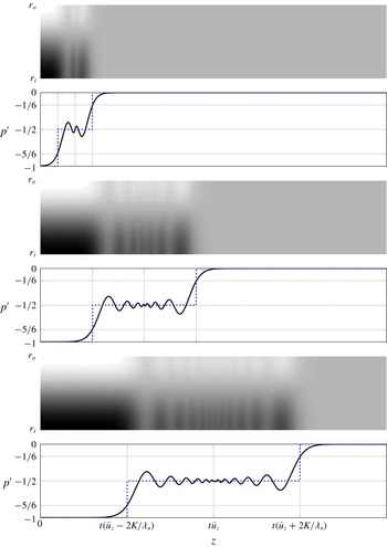
1 Introduction
The present study is motivated by observations of the propagation of azimuthal velocity perturbations in premixed swirl burners. A common assumption in the combustion dynamics community is that such perturbations, which determine the overall flame response to acoustic perturbations and thermo-acoustic stability, are convected by the mean flow. In several publications, however, propagation speeds approximately 40 %–50 % faster than the mean bulk flow velocity were reported, without further explanation. In this paper we explain these unexpected observations by recognizing azimuthal velocity perturbations as inertial waves, which obey a non-trivial dispersion relation. This introduction, therefore, starts with background on thermo-acoustic combustion instabilities – in particular the dynamics of swirl flames – and then makes a connection to the literature on inertial waves.
Thermo-acoustic instabilities arise from feedback between combustion system acoustics and unsteady heat release rate of the flame. This phenomenon was recognized in the late 19th century by Rayleigh (Reference Rayleigh1878), and played an important role in the development of rocket engines in the 1950s and 1960s (Culick Reference Culick, Culick, Heitor and Whitelaw1996; Poinsot Reference Poinsot2017). With the introduction of lean-premixed combustion technology in modern, low-emission gas turbines, thermo-acoustic combustion instabilities have again become a very active research area.
Modern combustion applications often employ aerodynamic swirl generators, which generate rotating flow upstream of the flame, in order to enhance flame stabilization and improve fuel mixing (Candel et al. Reference Candel, Durox, Schuller, Bourgouin and Moeck2014). Swirlers significantly influence the mean flame shape and the response of the flame to external perturbations (‘flame dynamics’) and hence the thermo-acoustic stability of the combustion system.
Richards and co-workers (Richards & Yip Reference Richards and Yip1995; Straub & Richards Reference Straub and Richards1999) observed that the axial position of the swirler in a premix burner had a significant impact on combustion stability, and put forward an explanation ‘related to variations in the azimuthal velocity being convected from the swirl vanes to the end of the nozzle’. These ‘tentative’ (to quote Richards) arguments were corroborated by Komarek & Polifke (Reference Komarek and Polifke2010) in a study that endeavoured to make explicit the effects of superposition of the respective flame responses to axial and azimuthal velocity perturbations on the overall flame transfer function. The burner used was designed such that the axial position of the swirler could be varied easily. Therefore, it was possible to change the relative phase between the respective contributions to the flame response. In confirmation of the arguments of Richards and co-workers it was observed that both gain and phase of the flame transfer function as well as stability limits depend in a very sensitive manner on the position of the swirl generator. (Note that results on the latter were reported only recently by Albayrak et al. (Reference Albayrak, Steinbacher, Komarek and Polifke2018b ).) The experimental results were supplemented by numerical simulation of the respective flame responses to axial and azimuthal velocity perturbations and the transport of azimuthal velocity perturbations from the swirler to the flame base. Phenomenological low-order models formulated in terms of (distributed) time delays for the transport of perturbations and the flame responses provided additional substantiation. In summary, Komarek & Polifke (Reference Komarek and Polifke2010) showed that the response of a swirl flame to azimuthal velocity perturbations generated at the swirler interferes with the response to axial fluctuations. The swirler position governs the relative phase between these contributions and thus decides whether superposition is constructive or destructive.
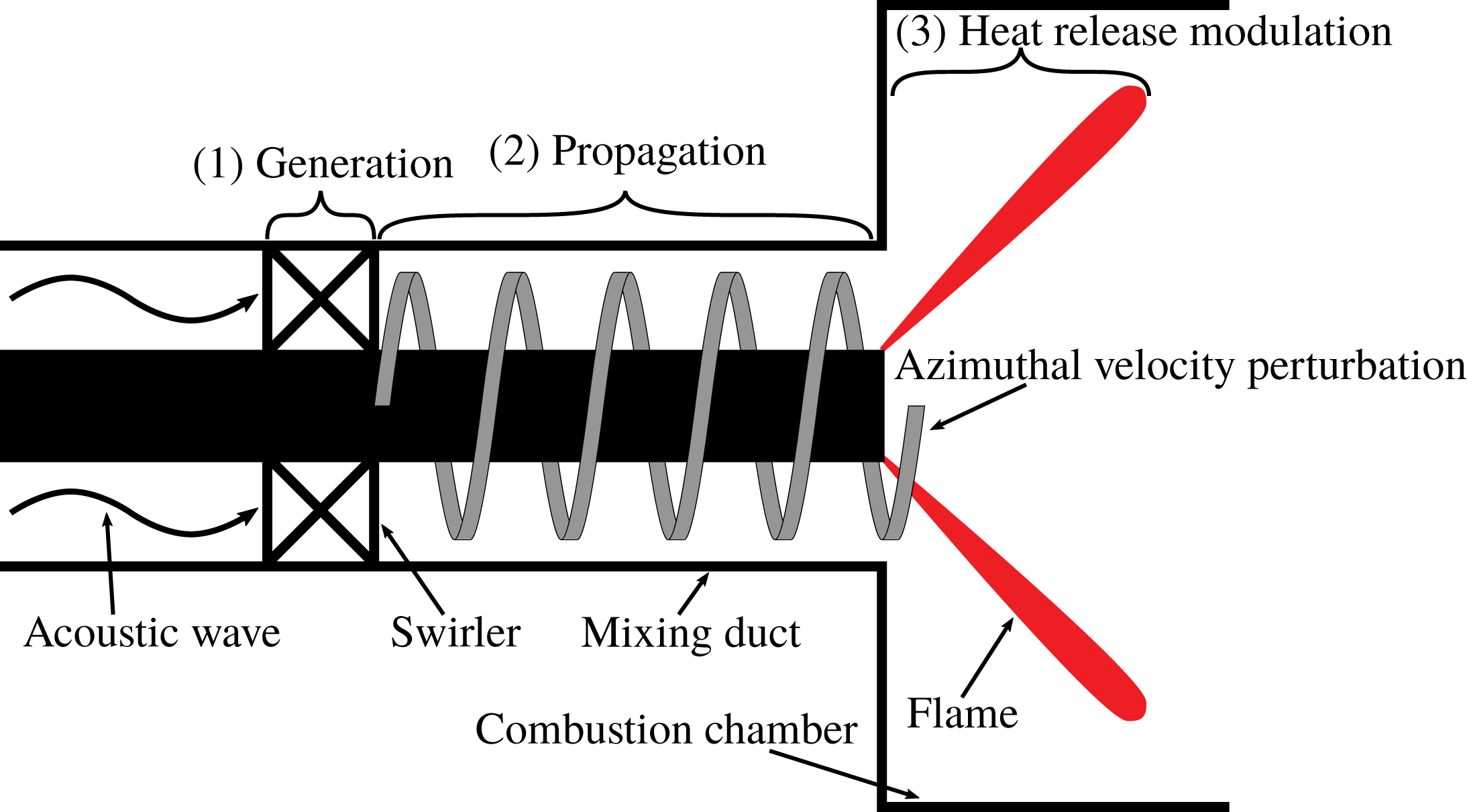
Schematic illustration of the interaction between azimuthal velocity fluctuations and the heat release rate in three consecutive steps. Firstly, acoustic waves generate azimuthal velocity fluctuations across the swirler via mode conversion. These fluctuations propagate inside the mixing duct towards the combustion chamber. Finally, the kinematic distortion in the flow–flame balance causes the heat release rate modulations.

Azimuthal velocity perturbations play a crucial role in the particular acoustic–flow–flame interaction mechanism outlined in the previous paragraph. A number of studies (see below) have investigated this mechanism, which can be analysed in three consecutive steps (as depicted in figure 1): firstly, the generation of azimuthal velocity fluctuations at the swirler, secondly, the propagation of these ‘vorticity waves’ or ‘swirl waves’ across the mixing duct to the flame base and, finally, modulation of the heat release rate by the azimuthal perturbations.
The first step can be regarded as an acoustic–convective mode conversion: acoustic waves incident on the swirler generate azimuthal velocity fluctuations. This process can be described by a model that is known in the turbomachinery community as the ‘actuator disk theory’, which delivers jump conditions across turbomachinery elements (Kaji & Okazaki Reference Kaji and Okazaki1970; Greitzer, Tan & Graf Reference Greitzer, Tan and Graf2004). Palies et al. (Reference Palies, Durox, Schuller and Candel2010, Reference Palies, Durox, Schuller and Candel2011a ) tailored the actuator disk model specifically to describe the generation of convective vorticity waves at a premix swirl burner and to discuss the implications for thermo-acoustic stability.
The exact mechanism of the third and final step, by which fluctuations of azimuthal velocity modulate the rate of heat release by the flame, has been a matter of debate since the seminal paper of Richards & Yip (Reference Richards and Yip1995). Indeed, several authors have endeavoured to identify the governing flow–flame interaction mechanisms and to quantify the flame response to swirl fluctuations. As explained by Acharya & Lieuwen (Reference Acharya and Lieuwen2014), the essential difficulty of the matter is that an axisymmetric flame is disturbed only by velocity components normal to it, thus there is no direct ‘disturbance pathway’ between azimuthal velocity fluctuations and flame heat release rate. Hirsch et al. (Reference Hirsch, Fanaca, Reddy, Polifke and Sattelmayer2005) argue that generation and stretching of azimuthal vorticity along diverging streamlines represents an indirect disturbance pathway between fluctuating circulation and flame heat release rate, and build a semi-analytical model based on the vorticity transport equation and the Biot–Savart law. Palies et al. (Reference Palies, Durox, Schuller and Candel2010) observe that fluctuations in swirl number ‘give rise to a breathing motion of the central recirculation region resulting in an angular deflection of the flame’. They comment that ‘This motion is equivalent to that which would be induced by perturbations of the burning velocity’ and indeed, the idea that ‘incident velocity modulations modify the swirl number and effectively change the turbulent burning velocity’ was explored in a follow-up study (Palies et al. Reference Palies, Schuller, Durox and Candel2011c ). Results obtained with numerical simulation of turbulent reacting flows by Acharya & Lieuwen (Reference Acharya and Lieuwen2014) show that ‘azimuthal flow fluctuations generate significant radial and axial flow fluctuations’, but the precise flow dynamics of this effect is not elaborated.
In contrast to the numerous publications on the first and third steps, a thorough analysis of the second step, i.e. the propagation of azimuthal velocity perturbations in the mixing duct, has not yet been carried out. This step is clearly important, because the time required for propagation from the swirler to the root of the flame governs the relative phase between the responses to axial and azimuthal velocity fluctuations. In the majority of publications cited above, the propagation is simply assumed to be convective, which indeed seems to be an entirely reasonable assumption for convective vortical waves. In a recent publication Palies, Ilak & Cheng (Reference Palies, Ilak and Cheng2017) employ the linearized Euler equations to argue that azimuthal velocity fluctuations propagate with the speed of convection. However, the analysis relies on merely the radial and azimuthal momentum equations and neglects the mass conservation and axial momentum equations. We will discuss the shortcomings of this approach in § 2.3.
However, in several studies it was mentioned that the assumption of convective propagation of azimuthal velocity perturbations does not agree quantitatively with experimental or computational findings. For example, Komarek & Polifke (Reference Komarek and Polifke2010) report that a match between a low-order model for the flame transfer function and experiment is achieved only if the convective velocity is set in an ad hoc manner to a value that exceeds the bulk velocity in the burner by approximately 40 %. Similarly, Palies et al. (Reference Palies, Durox, Schuller and Candel2011b
) report a propagation speed of
 $4.1~\text{m}~\text{s}^{-1}$
in an experiment with an axial swirl generator, while the bulk speed is
 $2.7~\text{m}~\text{s}^{-1}$
. Similar deviations are reported in the computational study of Acharya & Lieuwen (Reference Acharya and Lieuwen2014). These observations, which clearly imply that the propagation of azimuthal velocity fluctuations is not strictly convective, motivate the present work.
The goal of the present study is to further elucidate the physical characteristics of the propagation of azimuthal velocity fluctuations in cylindrical flow and to quantify the speed of propagation. For this purpose, we consider waves in rotating flows, i.e. inertial waves, also known as Kelvin waves due to the seminal work of Thomson (Reference Thomson1880). Inertial waves are dispersive waves that are driven by the restoring Coriolis force in swirling flows. Readers may refer standard textbooks for an introduction, e.g. Greenspan (Reference Greenspan1968), Saffman (Reference Saffman1993). Inertial waves play a role in various fields. Publications by Lessen, Singh & Paillet (Reference Lessen, Singh and Paillet1974), Gallaire & Chomaz (Reference Gallaire and Chomaz2003a ,Reference Gallaire and Chomaz b ) and Parras & Fernandez-Feria (Reference Parras and Fernandez-Feria2007) focused on hydrodynamic stability analysis of vortex cores. In these publications, the objective was to investigate the linear stability of various vortex types, e.g. the Rankine or Batchelor vortex, and identify a variety of wave modes, including inertial waves. A similar mathematical framework was used to study the vortex breakdown phenomenon. Benjamin (Reference Benjamin1962) developed the critical swirl state concept to estimate under which circumstances vortex breakdown may occur. The critical swirl represents the boundary between subcritical and supercritical flow states. The former accommodates standing waves, whereas the latter can only support downstream propagating waves. The occurrence of vortex breakdown is attributed to the subcritical region. Although not explicitly mentioned in Benjamin’s papers, these waves correspond to inertial waves. Rusak & Lee (Reference Rusak and Lee2002) extended this concept to estimate the impact of compressibility on the critical swirl. Confirmation was provided by Renac, Sipp & Jacquin (Reference Renac, Sipp and Jacquin2007) who derived an analytical asymptotic solution, where inertial wave dynamics was also identified.
Inertial waves play a role also in turbomachinery applications, e.g. Kerrebrock (Reference Kerrebrock1977), Golubev & Atassi (Reference Golubev and Atassi1998) and Tam & Auriault (Reference Tam and Auriault1998). These authors focused on acoustic wave modes in rotating duct flows for a range of Mach numbers and swirl strengths and characterized inertial waves as ‘nearly convected waves’.
The above mentioned publications are concerned with asymptotic stability of inertial wave modes. There are only a few attempts to investigate the spatio-temporal evolution of inertial waves. Arendt, Fritts & Andreassen (Reference Arendt, Fritts and Andreassen1997) proposed an initial value problem for a vortex tube, employing the linearized incompressible Euler equations for the Rankine vortex, where the flow is perturbed by an axial vortical disturbance as an initial condition. The time evolution is formed as a discrete superposition of inertial wave eigenmodes.
The present study follows a similar approach, but with important differences. Following Kerrebrock (Reference Kerrebrock1977), the azimuthal flow profile downstream of the swirler is assumed to be solid body rotation, which is simpler to investigate than the Rankine vortex considered by Arendt et al. (Reference Arendt, Fritts and Andreassen1997). The analytical handling of equations is easier and consequently time–space domain solutions are derived. The resultant solution is sufficiently simple that it contributes to the understanding of inertial wave dynamics and analytically quantifies the inertial wave propagation speed. Moreover, we consider an initial condition that corresponds to a perturbation generated by a plane acoustic wave propagating in the downstream direction across a swirler. Therefore, the initial value problem is written for compressible flows. The solution accounts for the dispersive wave structures, with propagation speeds that depend on mean flow properties – in particular swirl number – and may deviate significantly from the speed of convection. This outcome also explains the unexpected propagation speeds discussed above.
The modal analysis of inertial waves is introduced in § 2. We start with the compressible set of equations in § 2.1 to analyse the interaction between acoustics and inertial waves. Moreover, the compressible framework is necessary to identify the acoustic–convective mode conversion across the swirler. Well-known incompressible inertial wave modal properties are derived in § 2.2 from the compressible solution in the limit of the infinite sound speed. The interpretation of both compressible and incompressible modal analysis results is given in § 2.3, where the corresponding eigenvalues and eigenmode structures are discussed in detail. Section 2.4 compares analytical results with the numerical solution of the linearized Navier–Stokes equations. In § 3, the initial value problem is proposed, i.e. a step acoustic perturbation is imposed upstream of a swirler in an annular duct. The spatio-temporal evolution of waves after the swirler is analysed. The actuator disk theory is revised in § 3.1 to describe the generation of azimuthal velocity fluctuations from acoustic waves across the swirler. In § 3.2, using the actuator disk theory, the initial value conditions are derived for the acoustic step perturbation. Two different methods are proposed in § 3.3 to solve the initial value problem analytically, namely a non-dispersive low frequency and low wavenumber model and an asymptotic solution via the method of steepest descent. In § 4, these theoretical solutions are demonstrated on a swirl stabilized burner that was previously investigated by Komarek & Polifke (Reference Komarek and Polifke2010). This clarifies the observed deviation in propagation speeds of azimuthal velocity fluctuations by acknowledging inertial waves. The proposed solution not only contributes insight into inertial wave dynamics, but also has a strong impact on thermo-acoustic modelling by accurately predicting propagation speeds with only a few inputs, such as the mixing duct diameter and swirler angle.
2 Modal analysis of inertial waves in swirling flow
Inertial waves may be accurately modelled by linearized equations, since fluctuation amplitudes are small compared to bulk flow velocities (Greenspan Reference Greenspan1968). Stability analysis of the linearized equations may be realized by modal decomposition of flow quantities, e.g. for a variable,
 $q(z,r,t)$
,
 $$\begin{eqnarray}\displaystyle q(z,r,t)=\int _{-\infty }^{\infty }\int _{-\infty }^{\infty }\exp (-\text{i}\unicode[STIX]{x1D714}t+\text{i}kz)\hat{q}(k,r,\unicode[STIX]{x1D714})\,\text{d}\unicode[STIX]{x1D714}\,\text{d}k, & & \displaystyle\end{eqnarray}$$
where the Fourier transformation converts time to angular frequency,
 $t\rightarrow \unicode[STIX]{x1D714}$
, and similarly axial position to axial wavenumber,
 $z\rightarrow k$
. Modal decomposition reduces the partial differential equations to ordinary differential equations. If simple base flows are assumed, analytical solutions become feasible, which can contribute to the insight and physical understanding of wave mechanisms.
In linear stability analysis, the aim is to determine the imaginary part of the angular frequency or/and axial wavenumber, which indicates the growth rate of perturbations. Although the stability properties of inertial waves are not of interest in this work, as they are known to be stable, a modal approach is also employed here, since it reveals not only the stability, but also the structures and the velocities of inertial wave eigenmodes. In the next section, an initial value problem for inertial waves is formulated, where the eigenmodes are used to characterize the initial perturbation. Moreover, the group speed of inertial wave eigenmodes accounts for the deviations in the propagation speed of azimuthal velocity fluctuations from convection, as discussed in the introduction.
As demonstrated by several authors (Golubev & Atassi Reference Golubev and Atassi1998; Tam & Auriault Reference Tam and Auriault1998; Rusak & Lee Reference Rusak and Lee2002; Renac et al. Reference Renac, Sipp and Jacquin2007), the impact of compressibility on inertial waves can be neglected for low Mach number flows, as they are typically encountered in the mixing duct of premix burners. Nevertheless, we begin the following subsection with the modal analysis of compressible flow. The motivation behind this approach is the following: we shall demonstrate that plane acoustic waves propagating across a swirler generate inertial waves. The present study is limited to an axisymmetric analysis, since it is assumed that plane acoustic waves generate axisymmetric inertial wave modes. This assumption is justified by the observation that non-plane contributions to the perturbation, with mode orders that correspond e.g. to the number of flow passages of the swirler, decay quickly downstream of the swirler. To account for the acoustic waves, a compressible framework is required at this step. However, once inertial waves are generated, their subsequent evolution can be characterized in an incompressible framework. Therefore, incompressible inertial wave properties are also derived in § 2.2. Since the incompressible inertial waves are known in the fluid dynamics community, the derivation is realized as an asymptotic solution of the compressible equations in the limit of infinite speed of sound, instead of a traditional derivation starting from incompressible equations.
2.1 Compressible version
The Euler equations are the governing equations for inviscid compressible flow. Assuming isentropic flow, they are
 $$\begin{eqnarray}\displaystyle \frac{\unicode[STIX]{x2202}\unicode[STIX]{x1D70C}}{\unicode[STIX]{x2202}t}+\boldsymbol{u}\boldsymbol{\cdot }\unicode[STIX]{x1D735}\unicode[STIX]{x1D70C} & = & \displaystyle -\unicode[STIX]{x1D70C}\unicode[STIX]{x1D735}\boldsymbol{\cdot }\boldsymbol{u},\end{eqnarray}$$
 $$\begin{eqnarray}\displaystyle \frac{\unicode[STIX]{x2202}\boldsymbol{u}}{\unicode[STIX]{x2202}t}+\boldsymbol{u}\boldsymbol{\cdot }\unicode[STIX]{x1D735}\boldsymbol{u} & = & \displaystyle -\frac{1}{\unicode[STIX]{x1D70C}}\unicode[STIX]{x1D735}p,\end{eqnarray}$$
 $\unicode[STIX]{x1D70C}$
,
 $\boldsymbol{u}$
and
 $p$
stand for the density, velocity vector and pressure, respectively. Due to the isentropic assumption, a transport equation for energy is not required. In order to facilitate linearization, a simple cylindrical mean flow field in an annulus
 $r_{i}\leqslant r\leqslant r_{o}$
is considered
 $$\begin{eqnarray}\displaystyle \bar{\boldsymbol{u}}=[\bar{u}_{z},0,Kr], & & \displaystyle\end{eqnarray}$$
where
 $\bar{u}_{z}$
indicates the uniform axial velocity. The flow is in solid body rotation, such that the mean azimuthal velocity component
 $\bar{u}_{\unicode[STIX]{x1D703}}=Kr$
increases linearly with radius, where the circulation strength
 $K$
is – up to a factor
 $2\unicode[STIX]{x03C0}r_{o}^{2}$
– equal to the circulation of the flow. The mean pressure and density can be determined via the ideal gas law and the radial momentum balance, which are, respectively,
 $$\begin{eqnarray}\displaystyle \bar{p} & = & \displaystyle \frac{c^{2}}{\unicode[STIX]{x1D6FE}}\bar{\unicode[STIX]{x1D70C}},\end{eqnarray}$$
 $$\begin{eqnarray}\displaystyle \bar{\unicode[STIX]{x1D70C}}\frac{\bar{u}_{\unicode[STIX]{x1D703}}^{2}}{r} & = & \displaystyle \frac{\unicode[STIX]{x2202}\bar{p}}{\unicode[STIX]{x2202}r},\end{eqnarray}$$
 $c$
is the speed of sound and
 $\unicode[STIX]{x1D6FE}$
is the ratio of specific heats. Note that the isentropic relation is used in the ideal gas law. The radial profile of mean pressure is obtained as
 $$\begin{eqnarray}\displaystyle \bar{p}(r)=p_{0}\exp \left(\frac{\unicode[STIX]{x1D6FE}K^{2}r^{2}}{2c^{2}}\right) & & \displaystyle\end{eqnarray}$$
with reference pressure
 $p_{0}$
. The mean density profile can be trivially retrieved by substituting this relation back into the ideal gas law. Given the above mean fields, equation (2.2) is linearized as
 $$\begin{eqnarray}\displaystyle \frac{1}{c^{2}}\left(\frac{\unicode[STIX]{x2202}p^{\prime }}{\unicode[STIX]{x2202}t}+\bar{u}_{z}\frac{\unicode[STIX]{x2202}p^{\prime }}{\unicode[STIX]{x2202}z}\right) & = & \displaystyle -\displaystyle u_{r}^{\prime }\frac{\unicode[STIX]{x2202}\bar{\unicode[STIX]{x1D70C}}}{\unicode[STIX]{x2202}r}-\bar{\unicode[STIX]{x1D70C}}\left(\frac{\unicode[STIX]{x2202}u_{z}^{\prime }}{\unicode[STIX]{x2202}z}+\frac{\unicode[STIX]{x2202}u_{r}^{\prime }}{\unicode[STIX]{x2202}r}+\frac{u_{r}^{\prime }}{r}\right),\end{eqnarray}$$
 $$\begin{eqnarray}\displaystyle \frac{\unicode[STIX]{x2202}u_{z}^{\prime }}{\unicode[STIX]{x2202}t}+\bar{u}_{z}\frac{\unicode[STIX]{x2202}u_{z}^{\prime }}{\unicode[STIX]{x2202}z} & = & \displaystyle -\frac{1}{\bar{\unicode[STIX]{x1D70C}}}\frac{\unicode[STIX]{x2202}p^{\prime }}{\unicode[STIX]{x2202}z},\end{eqnarray}$$
 $$\begin{eqnarray}\displaystyle \frac{\unicode[STIX]{x2202}u_{r}^{\prime }}{\unicode[STIX]{x2202}t}+\bar{u}_{z}\frac{\unicode[STIX]{x2202}u_{r}^{\prime }}{\unicode[STIX]{x2202}z} & = & \displaystyle -\frac{1}{\bar{\unicode[STIX]{x1D70C}}}\frac{\unicode[STIX]{x2202}p^{\prime }}{\unicode[STIX]{x2202}r}+\displaystyle \frac{1}{c^{2}\bar{\unicode[STIX]{x1D70C}}^{2}}\frac{\unicode[STIX]{x2202}\bar{p}}{\unicode[STIX]{x2202}r}p^{\prime }+\frac{2\bar{u}_{\unicode[STIX]{x1D703}}u_{\unicode[STIX]{x1D703}}^{\prime }}{r},\end{eqnarray}$$
 $$\begin{eqnarray}\displaystyle \frac{\unicode[STIX]{x2202}u_{\unicode[STIX]{x1D703}}^{\prime }}{\unicode[STIX]{x2202}t}+\bar{u}_{z}\frac{\unicode[STIX]{x2202}u_{\unicode[STIX]{x1D703}}^{\prime }}{\unicode[STIX]{x2202}z} & = & \displaystyle -u_{r}^{\prime }\left(\frac{\text{d}\bar{u}_{\unicode[STIX]{x1D703}}}{\text{d}r}+\frac{\bar{u}_{\unicode[STIX]{x1D703}}}{r}\right),\end{eqnarray}$$
 $p^{\prime }=c^{2}\unicode[STIX]{x1D70C}^{\prime }$
, is employed to replace
 $\unicode[STIX]{x1D70C}^{\prime }$
with
 $p^{\prime }$
. The ratio between the azimuthal velocity at the outer radius
 $r_{o}$
and the speed of sound
 $c$
is defined as the swirling Mach number
 $$\begin{eqnarray}\displaystyle Ma_{s}=\frac{Kr_{o}}{c}. & & \displaystyle\end{eqnarray}$$
In the limit
 $Ma_{s}\ll 1$
, the impact of circulation on the mean pressure in (2.5) is negligible and the governing equations can be further simplified: uniform radial profiles of pressure and density may be assumed and the boxed terms in (2.6) may be neglected. Nevertheless, note that the set of equations resulting from the assumption
 $Ma_{s}\ll 1$
retains compressibility.
In the following, the condition of small swirling Mach number
 $Ma_{s}\ll 1$
is considered for the compressible flow case. In order to retrieve incompressible equations an additional assumption of infinitely fast speed of sound
 $c\rightarrow \infty$
is required. This step, which allows further simplifications, is performed in the next subsection.
Modal decomposition as defined in (2.1) simplifies the partial differential equations (2.6) to the following second-order ordinary differential equation for
 $\hat{u} _{r}$
as
 $$\begin{eqnarray}\displaystyle \frac{\text{d}^{2}\hat{u} _{r}}{\text{d}r^{2}}+\frac{1}{r}\frac{\text{d}\hat{u} _{r}}{\text{d}r}+\hat{u} _{r}\left(A^{2}-\frac{1}{r^{2}}\right)=0. & & \displaystyle\end{eqnarray}$$
The factor
 $A$
, which is introduced here for better readability, is defined as
 $$\begin{eqnarray}\displaystyle A=\sqrt{(C^{2}-4K^{2})\left(\frac{1}{c^{2}}-\frac{k^{2}}{C^{2}}\right)}, & & \displaystyle\end{eqnarray}$$
with modal convective operator
 $C$
,
 $$\begin{eqnarray}\displaystyle C=\unicode[STIX]{x1D714}-\bar{u}_{z}k. & & \displaystyle\end{eqnarray}$$
With impermeability boundary conditions at the inner and outer walls of the annulus,
 $$\begin{eqnarray}\displaystyle \hat{u} _{r}(r_{i}) & = & \displaystyle 0,\end{eqnarray}$$
 $$\begin{eqnarray}\displaystyle \hat{u} _{r}(r_{o}) & = & \displaystyle 0.\end{eqnarray}$$
 $$\begin{eqnarray}\displaystyle \hat{u} _{r}(r)=\unicode[STIX]{x1D705}_{1}[J_{1}(Ar)+\unicode[STIX]{x1D705}_{2}Y_{1}(Ar)], & & \displaystyle\end{eqnarray}$$
where
 $\unicode[STIX]{x1D705}_{2}$
and
 $A$
are found by applying the boundary conditions, while
 $\unicode[STIX]{x1D705}_{1}$
is to be determined via an initial condition. The boundary conditions inserted in the solution require
 $$\begin{eqnarray}\displaystyle J_{1}(Ar_{o})Y_{1}(Ar_{i})-J_{1}(Ar_{i})Y_{1}(Ar_{o})=0, & & \displaystyle\end{eqnarray}$$
where
 $J_{m}(r)$
and
 $Y_{m}(r)$
are the Bessel functions of first kind and second kind, respectively. As a characteristic property of the Sturm–Liouville theorem, this equation has infinitely many solutions with eigenvalues
 $\unicode[STIX]{x1D706}_{n}$
for the variable
 $A$
. The eigenvalues are ordered as
 $$\begin{eqnarray}\displaystyle \unicode[STIX]{x1D706}_{0}<\unicode[STIX]{x1D706}_{1}<\cdots <\unicode[STIX]{x1D706}_{n}<\cdots \rightarrow \infty . & & \displaystyle\end{eqnarray}$$
Substitution into (2.9) yields dispersion relations, which indicate how the frequencies
 $\unicode[STIX]{x1D714}_{n}$
of the corresponding eigenmodes depend on the wavenumber
 $k$
and the parameters
 $K,c$
that govern the mean flow,
 $$\begin{eqnarray}\displaystyle \unicode[STIX]{x1D714}_{n,i} & = & \displaystyle k\left(\bar{u}_{z}\pm \frac{c}{\sqrt{2}}\sqrt{L_{n}^{2}-\sqrt{L_{n}^{4}-\frac{16K^{2}}{k^{2}c^{2}}}}\right),\end{eqnarray}$$
 $$\begin{eqnarray}\displaystyle \unicode[STIX]{x1D714}_{n,a} & = & \displaystyle k\left(\bar{u}_{z}\pm \frac{c}{\sqrt{2}}\sqrt{L_{n}^{2}+\sqrt{L_{n}^{4}-\frac{16K^{2}}{k^{2}c^{2}}}}\right).\end{eqnarray}$$
 $i$
’ and ‘
 $a$
’ indicate inertial and acoustic eigenvalues, respectively. The non-dimensional parameter
 $L_{n}$
is written
 $$\begin{eqnarray}\displaystyle L_{n}=\sqrt{1+\left(\frac{\unicode[STIX]{x1D706}_{n}}{k}\right)^{2}+\left(\frac{2K}{ck}\right)^{2}}. & & \displaystyle\end{eqnarray}$$
Note that (2.15) is valid for
 $n\neq 0$
. For
 $n=0$
, i.e. the trivial solution
 $\unicode[STIX]{x1D706}_{0}=0$
, inertial waves do not exist and the well-known plane acoustic wave dispersion relation is recovered,
 $$\begin{eqnarray}\displaystyle \unicode[STIX]{x1D714}_{0,a}=k(\bar{u}_{z}\pm c). & & \displaystyle\end{eqnarray}$$
For both inertial and acoustic modes there exist two sets of solutions indicated by ‘
 $\pm$
’. The corresponding eigenmodes are determined by substituting the eigenvalues,
 $\unicode[STIX]{x1D706}_{n}$
, in (2.6) and written
 $$\begin{eqnarray}\displaystyle \hat{u} _{r,n}(r) & = & \displaystyle \unicode[STIX]{x1D705}_{1}M_{1}(\unicode[STIX]{x1D706}_{n}r),\end{eqnarray}$$
 $$\begin{eqnarray}\displaystyle \hat{u} _{\unicode[STIX]{x1D703},n}(r) & = & \displaystyle -\unicode[STIX]{x1D705}_{1}\frac{2K\text{i}}{C_{n}}M_{1}(\unicode[STIX]{x1D706}_{n}r),\end{eqnarray}$$
 $$\begin{eqnarray}\displaystyle \hat{u} _{z,n}(r) & = & \displaystyle \unicode[STIX]{x1D705}_{1}\frac{\text{i}kc^{2}\unicode[STIX]{x1D706}_{n}}{c^{2}k^{2}-C_{n}^{2}}M_{0}(\unicode[STIX]{x1D706}_{n}r),\end{eqnarray}$$
 $$\begin{eqnarray}\displaystyle \hat{p}_{n}(r) & = & \displaystyle \unicode[STIX]{x1D705}_{1}\frac{\text{i}C_{n}\bar{\unicode[STIX]{x1D70C}}c^{2}\unicode[STIX]{x1D706}_{n}}{c^{2}k^{2}-C_{n}^{2}}M_{0}(\unicode[STIX]{x1D706}_{n}r),\end{eqnarray}$$
 $$\begin{eqnarray}\displaystyle M_{m}(\unicode[STIX]{x1D706}_{n}r)=J_{m}(\unicode[STIX]{x1D706}_{n}r)-\frac{J_{1}(\unicode[STIX]{x1D706}_{n}r_{i})}{Y_{1}(\unicode[STIX]{x1D706}_{n}r_{i})}Y_{m}(\unicode[STIX]{x1D706}_{n}r). & & \displaystyle\end{eqnarray}$$
The modal convective operator is trivially extended for the
 $n$
th eigenmode as
 $$\begin{eqnarray}\displaystyle C_{n}=\unicode[STIX]{x1D714}_{n}-\bar{u}_{z}k. & & \displaystyle\end{eqnarray}$$
The interpretation of these results is presented in § 2.3 after the introduction of the incompressible modal analysis.
2.2 Incompressible version
Since the modal analysis of incompressible inertial waves is readily found in the literature (Greenspan Reference Greenspan1968), we will not repeat it in its traditional form. Instead, we demonstrate results as an asymptotic approach from the above compressible solution. This is accomplished by taking the limit of infinite speed of sound for each variable that is defined for the compressible case. From now on the superscript
 $\dagger$
is employed to indicate incompressible variables, i.e.
 $$\begin{eqnarray}\displaystyle q^{\dagger }=\lim _{c\rightarrow \infty }q. & & \displaystyle\end{eqnarray}$$
In the incompressibility limit, the linearized compressible equations as in (2.6) reduce to
 $$\begin{eqnarray}\displaystyle \frac{\unicode[STIX]{x2202}u_{z}^{\prime }}{\unicode[STIX]{x2202}z}+\frac{\unicode[STIX]{x2202}u_{r}^{\prime }}{\unicode[STIX]{x2202}r}+\frac{u_{r}^{\prime }}{r} & = & \displaystyle 0,\end{eqnarray}$$
 $$\begin{eqnarray}\displaystyle \frac{\unicode[STIX]{x2202}u_{z}^{\prime }}{\unicode[STIX]{x2202}t}+\bar{u}_{z}\frac{\unicode[STIX]{x2202}u_{z}^{\prime }}{\unicode[STIX]{x2202}z} & = & \displaystyle -\frac{1}{\bar{\unicode[STIX]{x1D70C}}}\frac{\unicode[STIX]{x2202}p^{\prime }}{\unicode[STIX]{x2202}z},\end{eqnarray}$$
 $$\begin{eqnarray}\displaystyle \frac{\unicode[STIX]{x2202}u_{r}^{\prime }}{\unicode[STIX]{x2202}t}+\bar{u}_{z}\frac{\unicode[STIX]{x2202}u_{r}^{\prime }}{\unicode[STIX]{x2202}z} & = & \displaystyle -\frac{1}{\bar{\unicode[STIX]{x1D70C}}}\frac{\unicode[STIX]{x2202}p^{\prime }}{\unicode[STIX]{x2202}r}+\frac{2\bar{u}_{\unicode[STIX]{x1D703}}u_{\unicode[STIX]{x1D703}}^{\prime }}{r},\end{eqnarray}$$
 $$\begin{eqnarray}\displaystyle \frac{\unicode[STIX]{x2202}u_{\unicode[STIX]{x1D703}}^{\prime }}{\unicode[STIX]{x2202}t}+\bar{u}_{z}\frac{\unicode[STIX]{x2202}u_{\unicode[STIX]{x1D703}}^{\prime }}{\unicode[STIX]{x2202}z} & = & \displaystyle -u_{r}^{\prime }\left(\frac{\text{d}\bar{u}_{\unicode[STIX]{x1D703}}}{\text{d}r}+\frac{\bar{u}_{\unicode[STIX]{x1D703}}}{r}\right).\end{eqnarray}$$
 $u_{r}^{\prime }$
can be written in the same form as (2.8)
 $$\begin{eqnarray}\displaystyle \frac{\text{d}^{2}\hat{u} _{r}}{\text{d}r^{2}}+\frac{1}{r}\frac{\text{d}\hat{u} _{r}}{\text{d}r}+\hat{u} _{r}\left((A^{\dagger })^{2}-\frac{1}{r^{2}}\right)=0, & & \displaystyle\end{eqnarray}$$
but the factor
 $A^{\dagger }$
reduces to
 $$\begin{eqnarray}\displaystyle A^{\dagger }=\frac{\text{i}k}{C}\sqrt{(C^{2}-4K^{2})}. & & \displaystyle\end{eqnarray}$$
In the incompressible limit, the propagation of the acoustic waves becomes non-local and thus its dispersion relation drops out and the inertial wave dispersion relation simplifies to
 $$\begin{eqnarray}\displaystyle \unicode[STIX]{x1D714}_{n,i}^{\dagger }=k\left(\bar{u}_{z}\pm \frac{2K}{kL_{n}^{\dagger }}\right). & & \displaystyle\end{eqnarray}$$
Now the non-dimensional parameter
 $L_{n}^{\dagger }$
is
 $$\begin{eqnarray}\displaystyle L_{n}^{\dagger }=\sqrt{1+\left(\frac{\unicode[STIX]{x1D706}_{n}}{k}\right)^{2}}. & & \displaystyle\end{eqnarray}$$
Corresponding eigenmodes are in the incompressible limit simplified to
 $$\begin{eqnarray}\displaystyle \hat{u} _{r,n}^{\dagger }(r) & = & \displaystyle \unicode[STIX]{x1D705}_{1}M_{1}(\unicode[STIX]{x1D706}_{n}r),\end{eqnarray}$$
 $$\begin{eqnarray}\displaystyle \hat{u} _{\unicode[STIX]{x1D703},n}^{\dagger }(r) & = & \displaystyle -\unicode[STIX]{x1D705}_{1}\frac{2K\text{i}}{C_{n}}M_{1}(\unicode[STIX]{x1D706}_{n}r),\end{eqnarray}$$
 $$\begin{eqnarray}\displaystyle \hat{u} _{z,n}^{\dagger }(r) & = & \displaystyle \unicode[STIX]{x1D705}_{1}\frac{\text{i}\unicode[STIX]{x1D706}_{n}}{k}M_{0}(\unicode[STIX]{x1D706}_{n}r),\end{eqnarray}$$
 $$\begin{eqnarray}\displaystyle \hat{p}_{n}^{\dagger }(r) & = & \displaystyle \unicode[STIX]{x1D705}_{1}\frac{\text{i}C_{n}\bar{\unicode[STIX]{x1D70C}}\unicode[STIX]{x1D706}_{n}}{k^{2}}M_{0}(\unicode[STIX]{x1D706}_{n}r).\end{eqnarray}$$
 $\unicode[STIX]{x1D706}_{n}$
are also identical and hence the dagger superscript may be omitted for the eigenvalues. Mode shapes are also the same as in the compressible case, but note that the prefactors are changed.
2.3 Interpretation of modal results
In this section, we interpret the results of modal analysis for both compressible and incompressible cases. In the literature, several publications present a similar analysis, but each of them focuses on different aspects. It is instructive to briefly discuss these studies and juxtapose our work.
For turbomachinery applications, Kerrebrock (Reference Kerrebrock1977) employed modal analysis to demonstrate wave modes in inviscid, compressible, ducted swirling flows. The author distinguished acoustic and ‘nearly convective’ waves and discussed the stability of modes. Golubev & Atassi (Reference Golubev and Atassi1998) extended this work by analysing a variety of azimuthal velocity profiles, i.e. free vortex
 $\bar{u}_{\unicode[STIX]{x1D703}}=\unicode[STIX]{x1D6E4}/r$
and solid body rotation
 $\bar{u}_{\unicode[STIX]{x1D703}}=Kr$
. They confirmed the existence of acoustic and nearly convective waves by means of asymptotic analysis and numerical solution of the modal equations with spectral methods. Kousen (Reference Kousen1996) followed a similar numerical approach. These studies mentioned also a third branch of ‘purely convective’ wave solutions for the free vortex case. Employing an initial value formulation, Tam & Auriault (Reference Tam and Auriault1998) confirmed the existence of the acoustic and nearly convected waves, but showed that the purely convective mode is a spurious mode, i.e. a numerical artefact.
Note that all of these early studies speak of ‘nearly convective’ waves. This term indicates that wave propagation is of dispersive character, with speeds close to those of convection by the mean flow – an order of magnitude slower than acoustic propagation. However, there were no further attempts to quantify the wave propagation velocities. The Coriolis force was correctly identified as the driving mechanism of these waves, however, there was no mention of the literature on inertial waves.
A modal analysis framework was also employed by Rusak & Lee (Reference Rusak and Lee2002) for a numerical investigation of vortex breakdown in compressible flows. Based on the concept of critical swirl introduced by Benjamin (Reference Benjamin1962), it was shown that vortex breakdown occurs at lower swirl strength as Mach number increases. Renac et al. (Reference Renac, Sipp and Jacquin2007) confirmed this numerical result by analytically deriving the inertial wave dispersion relation. By setting
 $k=0$
and
 $\unicode[STIX]{x1D714}=0$
in the dispersion relation, the impact of compressibility on the critical swirl strength was assessed. Interestingly, the result for the dispersion relation agrees with (2.15) in non-dimensional form, although different assumptions were employed: Renac et al. (Reference Renac, Sipp and Jacquin2007) assumed that the product of wavenumber
 $k$
and Mach number
 $Ma$
is small
 $k\,Ma\ll 1$
, whereas the present derivation is based on the assumption of small swirling Mach number, i.e.
 $Ma_{s}\ll 1$
.
In contrast to prior publications, the present study employs modal analysis in order to characterize the eigenmode structures and quantify propagation speeds. Our main objective is to derive a time–space domain solution of an initial value problem (see § 3), where an initial perturbation of swirling flow results from an acoustic wave that is incident on a swirler. The dispersion relation is especially important in this context because propagation speeds of perturbations can be deduced from the group speed,
 $c_{g}=\unicode[STIX]{x2202}\unicode[STIX]{x1D714}/\unicode[STIX]{x2202}k$
. The modal analysis is a crucial step before proceeding to the initial value problem, as initial perturbations are decomposed into eigenmodes. In this regard, the present analysis follows Arendt et al. (Reference Arendt, Fritts and Andreassen1997), who represent an initial vortical perturbation of an incompressible vortex tube as a superposition of the corresponding inertial wave eigenmodes. An extensive discussion with respect to this publication is given in § 3.
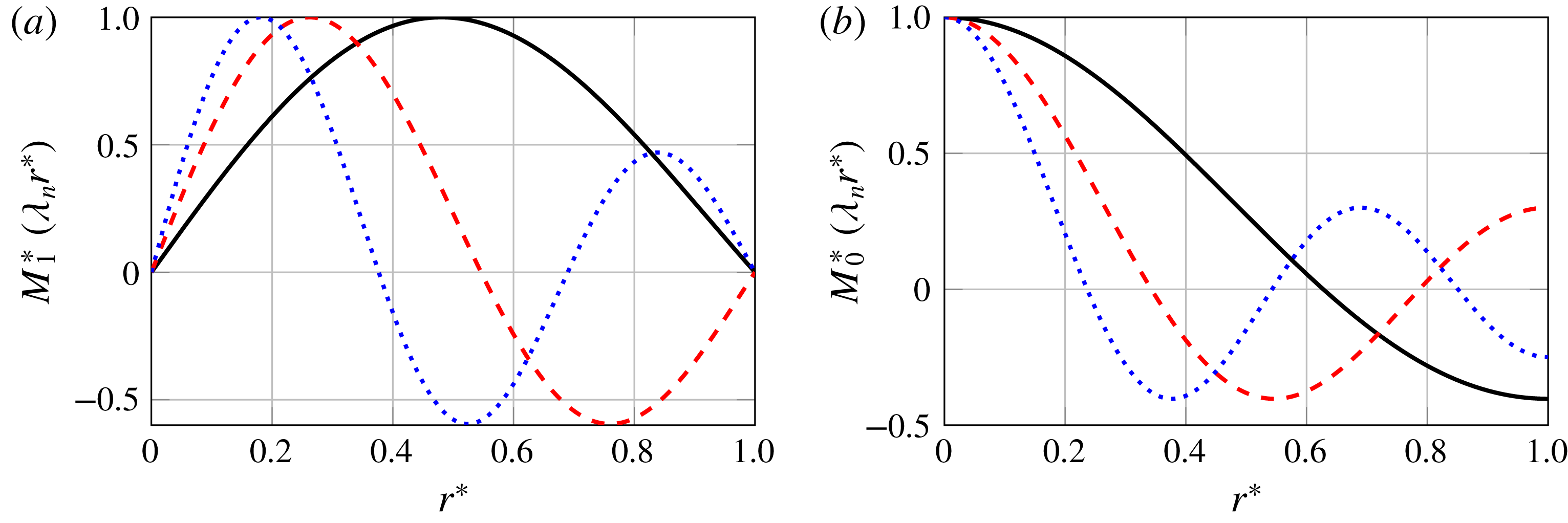
Structure of first three eigenmodes
 $n=1,2,3$
(solid black, dashed red, dotted blue lines). (a) Profiles of
 $\hat{u} _{\unicode[STIX]{x1D703}}$
and
 $\hat{u} _{r}$
as a function of radius. (b) Profiles of
 $\hat{u} _{z}$
and
 $\hat{p}$
.

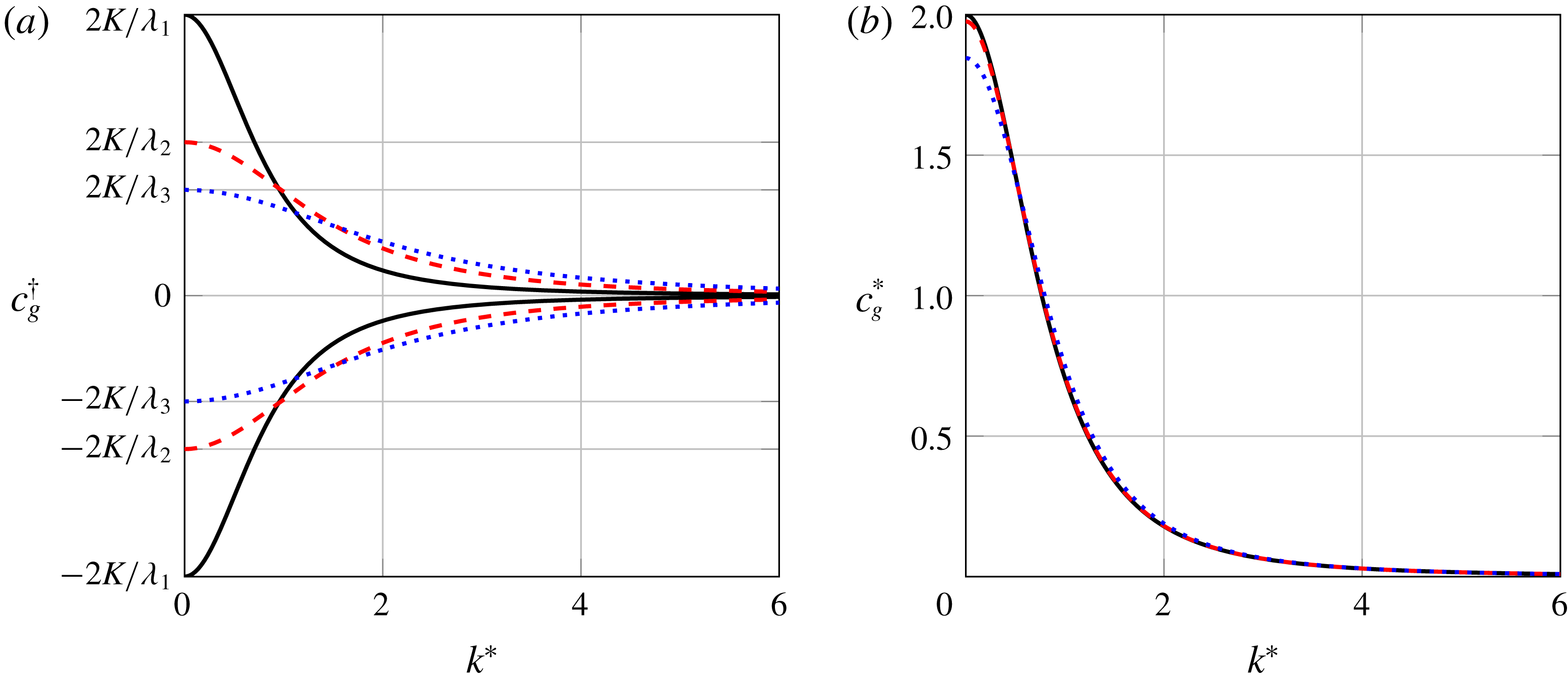
Inertial wave group speeds
 $c_{g}$
versus normalized axial wavenumber
 $k^{\ast }$
. (a) Incompressible case, reduced group speed
 $c_{g}^{\dagger }-\bar{u}_{z}$
of the first three eigenmodes
 $n=1,2,3$
(solid black, dashed red, dotted blue lines). (b) Comparison of incompressible (solid black line) and compressible normalized reduced group speeds
 $c_{g}^{\ast }$
for swirling Mach numbers
 $Ma_{s}=0.3$
(dashed red) and
 $Ma_{s}=0.8$
(dotted blue). Only first fast propagating group speed is considered.

Figure 2 shows radial profiles of the first three eigenmodes
 $n=1,2,3$
as defined in (2.18) and (2.27). Panel (a) shows profiles of radial and azimuthal velocities
 $\hat{u} _{r}$
and
 $\hat{u} _{\unicode[STIX]{x1D703}}$
, while panel (b) shows axial velocity
 $\hat{u} _{z}$
and pressure
 $\hat{p}$
. The radial coordinate is normalized as
 $r^{\ast }=(r-r_{i})/(r_{o}-r_{i})$
. The profiles are normalized with the respective maximum values, i.e.
 $M_{n}^{\ast }(\unicode[STIX]{x1D706}_{n}r^{\ast })=M_{n}(\unicode[STIX]{x1D706}_{n}r^{\ast })/\max (M_{n}(\unicode[STIX]{x1D706}_{n}r^{\ast }))$
. Note that the respective normalized profiles of the incompressible and the compressible cases agree with each other, thus the figure represents both cases. Obviously, the eigenmodes become more oscillatory with increasing order
 $n$
.
Figure 3 shows the dependence of inertial wave group speed on axial wavenumber. In these plots, reduced group speeds
 $c_{g}-\bar{u}_{z}$
are shown, i.e. the speed of convection is not taken into account. The wavenumber is normalized by the first eigenvalue,
 $k^{\ast }=k/\unicode[STIX]{x1D706}_{1}$
. Panel (a) represents the first three eigenmodes
 $n=1,2,3$
of the incompressible case. For each eigenmode, two values of the group speed are found, corresponding to the
 $\pm$
sign in the dispersion relations (2.15) and (2.25) for the compressible and the incompressible case, respectively. The opposite signs of the reduced group speeds
 $c_{g}-\bar{u}_{z}$
imply that inertial waves propagate at speeds above as well as below that of base flow convection. The deviation of the group speeds from the convective velocity increases with circulation strength
 $K$
, but diminishes with increasing order
 $n$
and with increasing axial wavenumber
 $k^{\ast }$
, indicative of dispersive wave propagation. In the low axial wavenumber limit, group speeds are the highest and are written
 $$\begin{eqnarray}\displaystyle \lim _{k\rightarrow 0}c_{g}^{\dagger }-\bar{u}_{z}=\pm \frac{2K}{\unicode[STIX]{x1D706}_{n}}. & & \displaystyle\end{eqnarray}$$
These values are shown on the ordinate of the plot.
These results provide an explanation for the unexpected experimental results on the propagation speed of azimuthal velocity perturbations that were discussed in the introduction. The 40 %–50 % deviation in the propagation speed from convection is attributed to dispersive inertial wave propagation. In § 3, an initial value problem is proposed for a detailed analysis and quantification of the inertial wave propagation.
Figure 3(b) shows the fast propagating group speed of the first eigenmode
 $n=1$
for values of the swirling Mach number
 $Ma_{s}=0,0.3,0.8$
, where the value of zero Mach number is represented by the solution for the incompressible case. The reduced group speeds are normalized
 $c_{g}^{\ast }=(c_{g}-\bar{u}_{z})\unicode[STIX]{x1D706}_{1}/K$
, such that the maximum group speed in the incompressible limit is
 $\lim _{c\rightarrow \infty }c_{g}^{\ast }=2$
. Obviously, the impact of compressibility on inertial wave propagation is marginal even for
 $Ma_{s}=0.8$
, which shows only a slight decrease in the group speed at small wavenumbers. This decrease can be quantified in the low wavenumber limit as
 $$\begin{eqnarray}\displaystyle \lim _{k\rightarrow 0}c_{g}-\bar{u}_{z}=\frac{2Kc}{\sqrt{\unicode[STIX]{x1D706}_{n}^{2}c^{2}+4K^{2}}}. & & \displaystyle\end{eqnarray}$$
Note that this solution implicitly confirms the compressibility dependency of the critical swirl state discussed by Rusak & Lee (Reference Rusak and Lee2002). The subcritical swirl state requires upstream propagating waves. By observing the above solution, this is satisfied for the following critical circulation strength as
 $$\begin{eqnarray}\displaystyle K_{c}=\frac{\bar{u}_{z}\unicode[STIX]{x1D706}_{n}c}{2\sqrt{c^{2}-\bar{u}_{z}^{2}}}. & & \displaystyle\end{eqnarray}$$
This condition agrees with the result of Renac et al. (Reference Renac, Sipp and Jacquin2007), i.e.
 $1/\sqrt{1-Ma^{2}}$
in non-dimensional form. The value
 $Ma_{s}=0.8$
seems incompatible with the assumption of small swirl Mach number, but note that this large value was selected to demonstrate that the change in the group speed is negligible. Also note that Renac et al. (Reference Renac, Sipp and Jacquin2007) provide a comparison against numerical solutions where the low Mach number assumption is relaxed. A good match is achieved, which confirms the validity of the results obtained with
 $Ma_{s}=0.8$
.
As mentioned in the introduction, Palies et al. (Reference Palies, Ilak and Cheng2017) employed linearized Euler equations to show that the propagation of azimuthal velocity perturbations is entirely convective. However, instead of using the complete set of Euler equations (2.6), only the radial and azimuthal momentum equations are taken into account (see equations (A 1) and (A 2) in Palies et al. (Reference Palies, Ilak and Cheng2017)), while mass conservation and the axial momentum equation are neglected. In the light of the present analysis, we argue that this incomplete set of equations is not capable of correctly describing inertial wave propagation, and that conclusions based upon these equations are invalid.
2.4 Comparison of inviscid theory against modal linearized Navier–Stokes equations
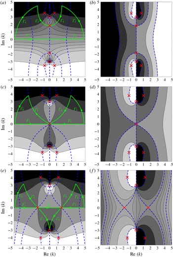
In this section, analytical results for the inviscid case are compared against numerical modal analysis based on the linearized incompressible Navier–Stokes equations. This comparison serves not only as validation, but also allows us to investigate the effects of viscosity on inertial waves. We employ an approach used previously in stability/sensitivity analysis (see Juniper (Reference Juniper2012) and Juniper, Hanifi & Theofilis (Reference Juniper, Hanifi and Theofilis2014)). In a flow that is not absolutely unstable, there is a convenient and reasonably accurate mapping between the temporal and spatial analyses at a given wavenumber or angular frequency (see Gaster (Reference Gaster1962)). Here, we perform a temporal analysis. The Chebyshev spectral collocation technique proposed by Khorrami, Malik & Ash (Reference Khorrami, Malik and Ash1989) is employed. A total of
 $50$
grid points are used for the discretization. The simplified flow field described in (2.3) is also employed for this numerical study. Slip wall boundary conditions are used to match the analytical inviscid approach accurately,
 $$\begin{eqnarray}\displaystyle \hat{u} _{r}=\hat{u} _{\unicode[STIX]{x1D703}}=\frac{\unicode[STIX]{x2202}\hat{u} _{z}}{\unicode[STIX]{x2202}r}=\frac{\unicode[STIX]{x2202}\hat{p}}{\unicode[STIX]{x2202}r}=0,\quad \text{for}~r=r_{i},r_{o}. & & \displaystyle\end{eqnarray}$$
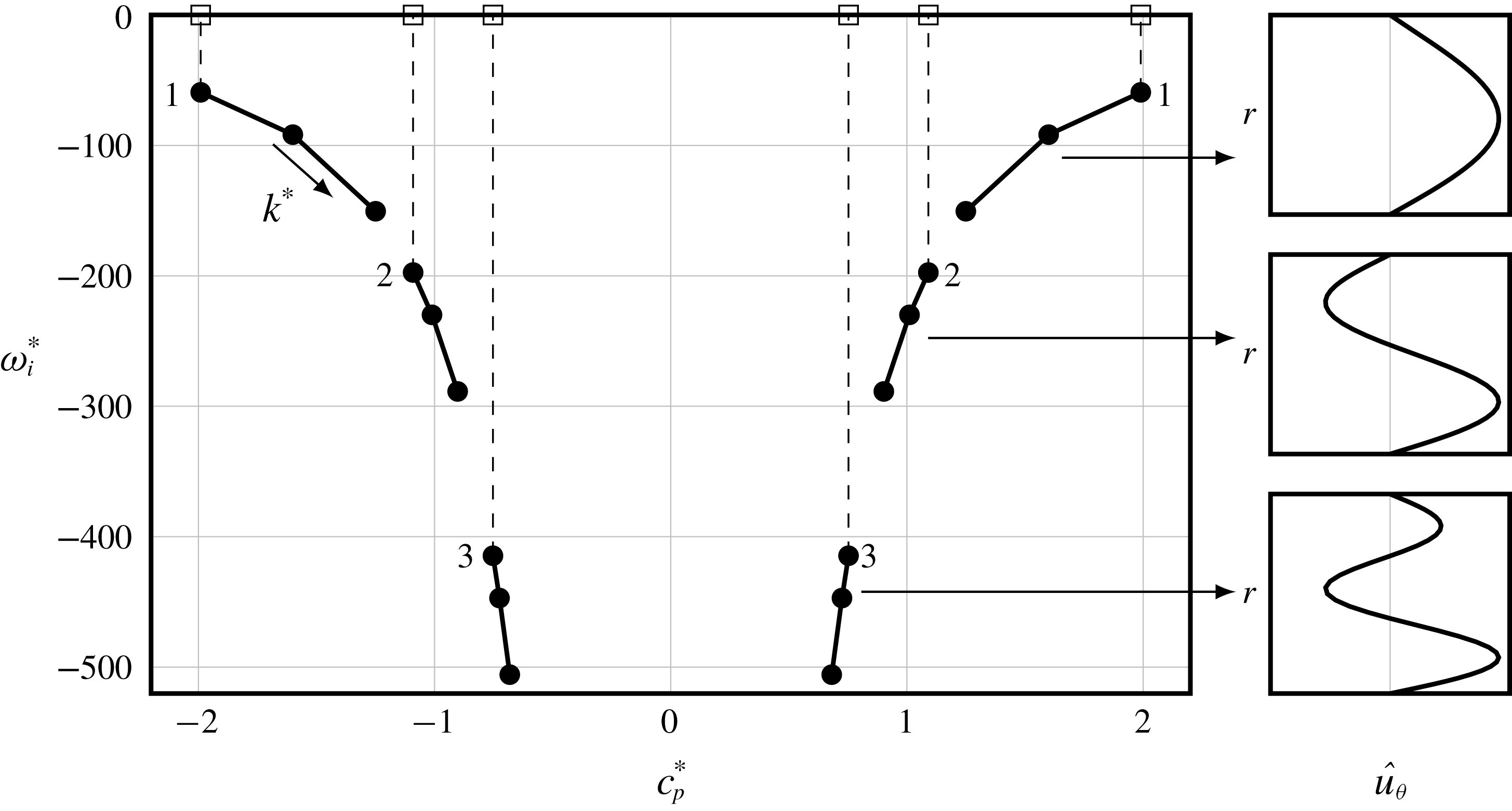
In figure 4, the eigenfrequencies
 $\unicode[STIX]{x1D714}_{n}$
of the first three modes
 $n=1,2,3$
are represented in terms of the respective phase speeds and growth rates for three values of axial wavenumber
 $k$
. The Reynolds number is selected as
 $Re=\bar{u}_{z}D_{H}/\unicode[STIX]{x1D708}=18\,000$
to match with the experimental configuration of Komarek & Polifke (Reference Komarek and Polifke2010), where
 $D_{H}$
is the hydraulic diameter and
 $\unicode[STIX]{x1D708}$
is the kinematic viscosity. Similarly, the swirl number is chosen as
 $S=KD_{H}/\bar{u}_{z}=1.6$
. However, owing to the non-dimensionalization described below, the results in figure 4 are independent of both these parameters.
Normalized temporal decay rate
 $\unicode[STIX]{x1D714}_{i}^{\ast }$
of the first six eigenvalues as a function of the normalized phase speed
 $c_{p}^{\ast }$
. Dots represent the temporal analysis for the linearized Navier–Stokes equation for three normalized axial wavenumbers,
 $k^{\ast }=[0.1,0.75,1.25]$
, which are connected by lines. Squares indicate the eigenvalues from the inviscid analysis as in (2.25) for
 $k^{\ast }=0.1$
. The corresponding radial profiles of azimuthal velocity perturbation are shown on the right.

The phase speed
 $c_{p}=\unicode[STIX]{x1D714}_{r}/k$
depends on the real part
 $\unicode[STIX]{x1D714}_{r}$
of the angular frequency. The abscissa of the plot corresponds to a normalized reduced phase speed, i.e.
 $c_{p}^{\ast }=(c_{p}-\bar{u}_{z})\unicode[STIX]{x1D706}_{1}/K$
, i.e. again, the plot represents the deviation from the speed of convection. The ordinate corresponds to the normalized decay rate,
 $\unicode[STIX]{x1D714}_{i}^{\ast }=\unicode[STIX]{x1D714}_{i}ReD_{H}/\bar{u}_{z}$
, i.e. the imaginary part of the angular frequency. Negative values indicate that the mode amplitude decays in time. Round markers represent eigenvalues calculated by the linearized Navier–Stokes equations. Solid lines are used to track eigenvalues for varying axial wavenumber. Squares represent analytical eigenvalues determined from the incompressible dispersion relation via (2.25). For a better visualization, the analytical eigenvalues are plotted only for
 $k^{\ast }=0.1$
. In figure 2(b), azimuthal velocity profiles of the eigenmodes are shown. Since analytical inviscid eigenmode profiles, which are shown in figure 2, are in perfect agreement with the numerical approach for the linearized Navier–Stokes equations, only a single mode profile is plotted. The arrows indicate which eigenmode corresponds to which set of eigenvalues. For each eigenmode, two eigenvalues exist, one being faster and the other being slower than the convection speed. Therefore, the eigenvalues are numbered as pairs. Inviscid phase speeds are also in perfect agreement with the numerical viscous approach. The obvious mismatch in decay rates is expected, since the inviscid analysis does not account for viscous dissipation.
The first pair of eigenvalues, i.e.
 $n=1$
, decays slowest and deviates most from the convective speed. With increasing mode order
 $n$
or wavenumber
 $k$
, the phase speeds approach the convection speed. These statements were also confirmed in the previous section for the inviscid approach. More importantly, modes are more strongly damped with increasing
 $n$
and
 $k$
. This trend in decay rates suggest that the low wavenumber region is more relevant for the propagation of a perturbation, with the first mode as the leading term, while high-order modes decay more rapidly. We shall use these findings to interpret the inertial wave propagation in thermo-acoustic systems, see § 4.
3 Inertial wave step response to acoustic perturbation
In this section, the time evolution of inertial waves is discussed in terms of an initial value problem. The methodology used here is inspired by Arendt et al. (Reference Arendt, Fritts and Andreassen1997), who investigated the temporal evolution of inertial waves observed in a vortex tube. In that study an initial value problem was formulated by introducing various perturbations in vorticity components on the linearized incompressible Euler equations. Although no closed form expressions in the time–space domain were derived, snapshots of instantaneous vorticity fields were demonstrated. By interpreting these results, the dynamics of inertial waves in the time domain was elucidated.
The approach followed in the present study is different in several regards. Firstly, a simpler base azimuthal velocity profile is considered, i.e. solid body rotation instead of the Rankine vortex. Hence, we are able to provide a closed form analytical solution in the time–space domain, which provides a better understanding. The choice of a simpler base flow profile is justified by the fact that the flow after a swirler is very close to solid body rotation (Kerrebrock Reference Kerrebrock1977). Since the flow in most combustion applications is highly turbulent, Ekman layers, i.e. boundary effects, are neglected and the rotation profile approaches to the solid body rotation as it is a stable state for rotating flows.
Secondly, Arendt et al. (Reference Arendt, Fritts and Andreassen1997), chose a Gaussian distribution in the axial direction as the initial perturbation of vorticity, with a width equal to the radius. This assumption introduces a cutoff in axial wavenumber, i.e. waves with a wavelength shorter than the width of the Gaussian profile are not resolved. This can be also interpreted as an arbitrary initial dispersion. However, such an assumption is not suitable in the present context, since the proposed initial perturbation is a plane acoustic wave, which is non-dispersive in nature. Therefore, we employ a Heaviside step function for the initial perturbation. This can be physically interpreted as a sudden jump (‘step perturbation’). Unlike the Gaussian distribution, the Heaviside function covers the entire frequency spectrum and thus describes non-dispersive plane acoustic waves. Moreover, entire wavelengths for inertial waves are resolved and more detailed results are obtained. The corresponding solution is formally called the ‘step response’, which is commonly used in control theory. The reader may consult standard control theory textbooks for further details. One other benefit of the step response is that it can be directly connected in an acoustic network model (Munjal Reference Munjal2014), which is the state-of-the-art modelling approach to predict thermo-acoustic instabilities.
The initial value problem employs Laplace transformation for time and Fourier transformation for the axial direction. For a variable
 $q(z,r,t)$
,
 $$\begin{eqnarray}\displaystyle q(z,r,t)=\int _{-\infty }^{\infty }\int _{0}^{\infty }\exp (-st+\text{i}kz)\hat{q}(k,r,s)\,\text{d}s\,\text{d}k. & & \displaystyle\end{eqnarray}$$
This transformation is similar to the modal decomposition as defined in (2.1), however Laplace transformation for time additionally requires an initial value for each quantity, e.g.
 $u_{\unicode[STIX]{x1D703}}^{\prime }(t=0)$
. The simplified linearized compressible Euler equations as defined in (2.6) are written after transformation as
 $$\begin{eqnarray}\displaystyle \frac{1}{c^{2}}[-\text{i}C\hat{p}-p^{\prime }(k,r,t=0)] & = & \displaystyle -\bar{\unicode[STIX]{x1D70C}}\left(\text{i}k\hat{u} _{z}+\frac{\unicode[STIX]{x2202}u_{r}^{\prime }}{\unicode[STIX]{x2202}r}+\frac{u_{r}^{\prime }}{r}\right),\end{eqnarray}$$
 $$\begin{eqnarray}\displaystyle -\text{i}C\hat{u} _{z}-u_{z}^{\prime }(k,r,t=0) & = & \displaystyle -\frac{\text{i}k}{\bar{\unicode[STIX]{x1D70C}}}\hat{p},\end{eqnarray}$$
 $$\begin{eqnarray}\displaystyle -\text{i}C\hat{u} _{r}-u_{r}^{\prime }(k,r,t=0) & = & \displaystyle -\frac{1}{\bar{\unicode[STIX]{x1D70C}}}\frac{\unicode[STIX]{x2202}\hat{p}}{\unicode[STIX]{x2202}r}+\frac{2\bar{u}_{\unicode[STIX]{x1D703}}\hat{u} _{\unicode[STIX]{x1D703}}}{r},\end{eqnarray}$$
 $$\begin{eqnarray}\displaystyle -\text{i}C\hat{u} _{\unicode[STIX]{x1D703}}-u_{\unicode[STIX]{x1D703}}^{\prime }(k,r,t=0) & = & \displaystyle -\hat{u} _{r}\left(\frac{\text{d}\bar{u}_{\unicode[STIX]{x1D703}}}{\text{d}r}+\frac{\bar{u}_{\unicode[STIX]{x1D703}}}{r}\right).\end{eqnarray}$$
 $\hat{u} _{r}$
as
 $$\begin{eqnarray}\displaystyle \frac{\text{d}^{2}\hat{u} _{r}}{\text{d}r^{2}}+\frac{1}{r}\frac{\text{d}\hat{u} _{r}}{\text{d}r}+\hat{u} _{r}\left(A^{2}-\frac{1}{r^{2}}\right) & = & \displaystyle \left(\frac{k^{2}}{C^{2}}-\frac{1}{c^{2}}\right)[2Ku_{\unicode[STIX]{x1D703}}^{\prime }(k,r,t=0)-\text{i}Cu_{r}^{\prime }(k,r,t=0)]\nonumber\\ \displaystyle & & \displaystyle +\,\frac{k}{C}\frac{\unicode[STIX]{x2202}u_{z}^{\prime }(k,r,t=0)}{\unicode[STIX]{x2202}r}+\frac{1}{\bar{\unicode[STIX]{x1D70C}}c^{2}}\frac{\unicode[STIX]{x2202}p^{\prime }(k,r,t=0)}{\unicode[STIX]{x2202}r}.\end{eqnarray}$$
The right-hand side of this equation describes initial value conditions. The homogeneous part of this equation is very similar to the modal decomposed equation (2.8) as described in the previous section. The only difference is the modal convective operator, which is redefined here as
 $$\begin{eqnarray}\displaystyle C=\text{i}s-k\bar{u}_{z}. & & \displaystyle\end{eqnarray}$$
For the incompressible flow, equation (3.3) reduces to
 $$\begin{eqnarray}\displaystyle \frac{\text{d}^{2}\hat{u} _{r}}{\text{d}r^{2}}+\frac{1}{r}\frac{\text{d}\hat{u} _{r}}{\text{d}r}+\hat{u} _{r}\left((A^{\dagger })^{2}-\frac{1}{r^{2}}\right) & = & \displaystyle \frac{k^{2}}{C^{2}}[2Ku_{\unicode[STIX]{x1D703}}^{\prime }(k,r,t=0)-\text{i}Cu_{r}^{\prime }(k,r,t=0)]\nonumber\\ \displaystyle & & \displaystyle +\,\frac{k}{C}\frac{\unicode[STIX]{x2202}u_{z}^{\prime }(k,r,t=0)}{\unicode[STIX]{x2202}r}.\end{eqnarray}$$
In order to solve this inhomogeneous ordinary differential equation, the initial conditions should be defined. Note that these equations are written for a general case, i.e. any kind of perturbation can be defined at this point. In this paper, we focus on thermo-acoustic applications. Therefore, the initial perturbation is assumed to originate from an acoustic wave, which is propagating across a swirler in the downstream direction. As discussed in the introduction, this acoustic wave generates an azimuthal velocity perturbation across the swirler at its downstream side, which should be regarded as an initial condition. In the next subsection, this mode conversion process is derived via the actuator disk theory. Jump conditions across the swirler by Palies et al. (Reference Palies, Durox, Schuller and Candel2011a ) are revisited by respecting the Coriolis force in the radial momentum balance.
3.1 Mode conversion: actuator disk theory
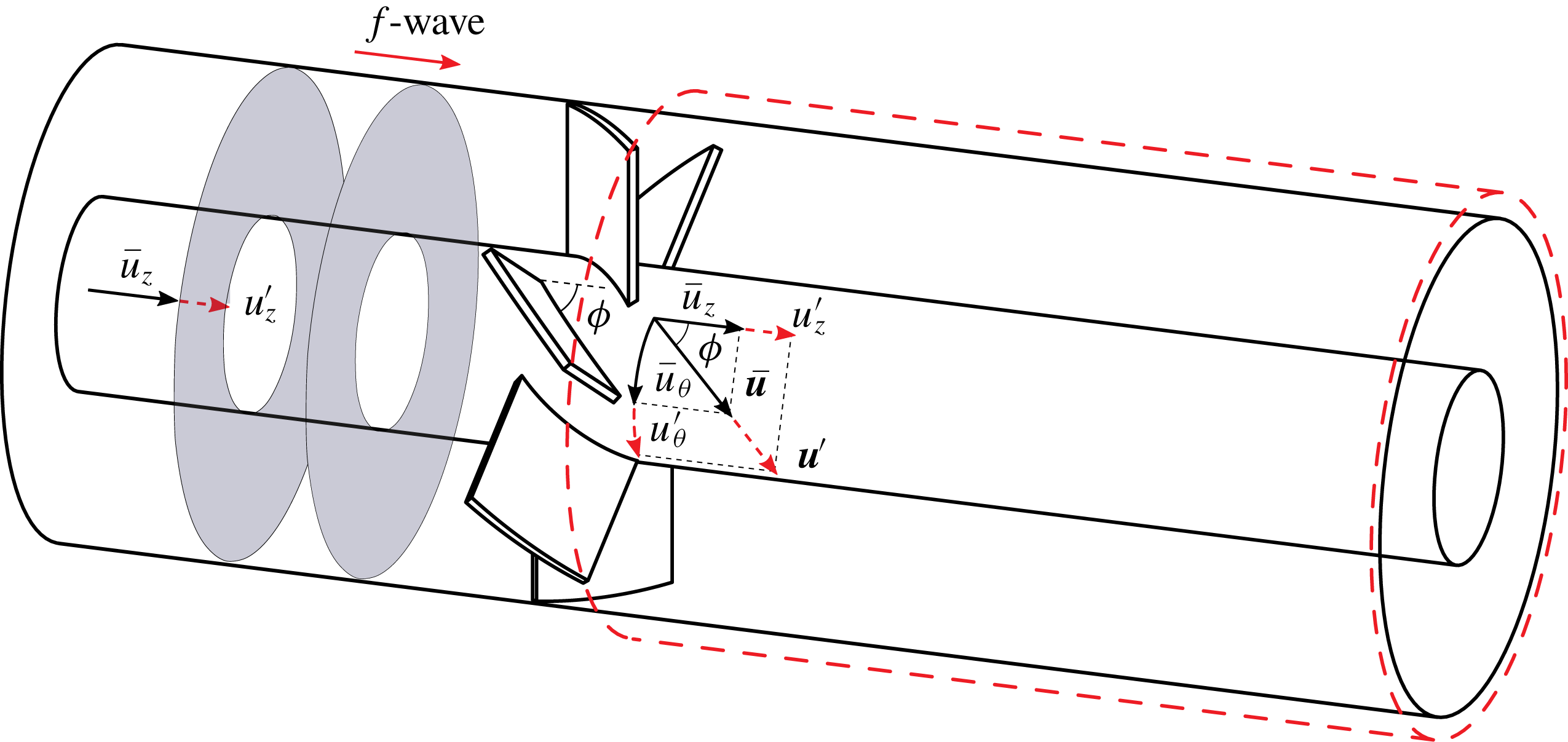
The mode conversion process across a swirler from incident plane acoustic waves to azimuthal velocity fluctuations was modelled via actuator disk theory by Cumpsty & Marble (Reference Cumpsty and Marble1977) and revised by Palies et al. (Reference Palies, Durox, Schuller and Candel2011a ) for thermo-acoustic applications. Here, we briefly introduce actuator disk theory and the set-up that we use for the initial value problem. The swirler is modelled as a thin disk that generates azimuthal momentum instantly. The jump condition across the swirler is schematically illustrated in figure 5. Solid black and dashed red arrows indicate the base and perturbed flow quantities, respectively. Grey planes represent upstream perturbations in downstream propagating plane acoustic waves.
Schematic illustration of the swirler inside an annular mixing duct. Grey planes indicate initial perturbations of downstream propagating acoustic waves as denoted by
 $f$
-waves. The base flow vectors are shown with solid black vectors. Right after the swirler, the mode conversion process is illustrated. Corresponding dashed red flow vectors indicate perturbed velocities resulting from actuator disk theory. The dashed red box indicates the domain for the initial value problem.

To derive jump conditions for small fluctuating quantities, Palies et al. (Reference Palies, Durox, Schuller and Candel2011a ) introduced several simplifications, which are also employed here: the flow is assumed to be isentropic, while the pressure drop across the swirler is neglected. Moreover, the swirler is assumed to be acoustically transparent, which means that the incident plane acoustic waves are transmitted in a lossless manner across the swirler. Under these assumptions, jump conditions are written as
 $$\begin{eqnarray}\displaystyle f|_{down} & = & \displaystyle f|_{up},\end{eqnarray}$$
 $$\begin{eqnarray}\displaystyle u_{\unicode[STIX]{x1D703}}^{\prime }|_{down} & = & \displaystyle u_{z}^{\prime }|_{up}\tan (\unicode[STIX]{x1D719}),\end{eqnarray}$$
 $f$
indicates the downstream propagating plane acoustic wave (see Rienstra & Hirschberg (Reference Rienstra and Hirschberg2018) for a formal definition). The second equation is derived via the Kutta condition, which states that the flow angle follows the solid angle at the trailing edge, as illustrated by the flow vectors in figure 5. Since the swirler is acoustically transparent, the downstream axial velocity perturbation is the same as the upstream acoustic velocity perturbation. At the same time, the flow direction, which is indicated by
 $\bar{\boldsymbol{u}}$
, should not change. Hence, this should be fulfilled via a perturbation in the azimuthal velocity.
In summary, plane acoustic waves incident on a swirler generate azimuthal velocity perturbations with a strength that depends on the swirler blade angle. From this point onward, mere convective transport of azimuthal velocity perturbations (also referred to as ‘vorticity waves’) has been taken for granted (Cumpsty & Marble Reference Cumpsty and Marble1977; Richards & Yip Reference Richards and Yip1995; Komarek & Polifke Reference Komarek and Polifke2010; Palies et al. Reference Palies, Durox, Schuller and Candel2011a ). Signal propagation times observed in experiments and simulations do not support this assumption, however, as discussed in the introduction, and no further attempts have been made until now to characterize the subsequent propagation of azimuthal velocity perturbations.
Another important point is that the Coriolis force has not been taken into consideration. Indeed, Palies et al. (Reference Palies, Durox, Schuller and Candel2011a ) simply used the one-dimensional plane acoustic wave solution, i.e.
 $$\begin{eqnarray}\displaystyle f & = & \displaystyle 0.5\left(\frac{p^{\prime }}{\bar{\unicode[STIX]{x1D70C}}c}+u_{z}^{\prime }\right),\end{eqnarray}$$
 $$\begin{eqnarray}\displaystyle g & = & \displaystyle 0.5\left(\frac{p^{\prime }}{\bar{\unicode[STIX]{x1D70C}}c}-u_{z}^{\prime }\right).\end{eqnarray}$$
 $g$
-wave propagating in the upstream direction is neglected by setting
 $g=0$
. Corresponding jump conditions for pressure and axial velocity fluctuations reduce to
 $$\begin{eqnarray}\displaystyle u_{z}^{\prime }|_{down} & = & \displaystyle f|_{up},\end{eqnarray}$$
 $$\begin{eqnarray}\displaystyle p^{\prime }|_{down} & = & \displaystyle \bar{\unicode[STIX]{x1D70C}}cf|_{up}.\end{eqnarray}$$
 $$\begin{eqnarray}\displaystyle p^{\prime }|_{down}=\bar{\unicode[STIX]{x1D70C}}cf|_{up}+2K\bar{\unicode[STIX]{x1D70C}}\int u_{\unicode[STIX]{x1D703}}^{\prime }|_{down}\,\text{d}r. & & \displaystyle\end{eqnarray}$$
This additional term is crucial for the compressible initial value problem (see (3.3)), but does not play a role in the incompressible case (see (3.5)). These assertions will be explained further in the next section.
3.2 Initial perturbation
To pose an initial value problem for inertial wave propagation, a step perturbation is introduced, as discussed in the previous subsection. This condition is written mathematically as
 $$\begin{eqnarray}\displaystyle u_{z}^{\prime }(z,r,t=0)|_{up} & = & \displaystyle \unicode[STIX]{x1D700}_{a}\text{H}(-z),\end{eqnarray}$$
 $$\begin{eqnarray}\displaystyle p^{\prime }(z,r,t=0)|_{up} & = & \displaystyle \unicode[STIX]{x1D700}_{a}\bar{\unicode[STIX]{x1D70C}}c\text{H}(-z),\end{eqnarray}$$
 $\unicode[STIX]{x1D700}_{a}$
is a small number that indicates the acoustic perturbation amplitude. The Heaviside function is
 $\text{H}(-z)$
, where the minus sign indicates that the initial perturbation is valid for
 $z<0$
. By employing actuator disk conditions from the previous section, the initial perturbation for the azimuthal velocity is written
 $$\begin{eqnarray}\displaystyle u_{z}^{\prime }(z,r,t=0)|_{down} & = & \displaystyle \unicode[STIX]{x1D700}_{a}\text{H}(-z),\end{eqnarray}$$
 $$\begin{eqnarray}\displaystyle u_{r}^{\prime }(z,r,t=0)|_{down} & = & \displaystyle 0,\end{eqnarray}$$
 $$\begin{eqnarray}\displaystyle u_{\unicode[STIX]{x1D703}}^{\prime }(z,r,t=0)|_{down} & = & \displaystyle \left(\mathop{\sum }_{n=1}^{\infty }\unicode[STIX]{x1D6FC}_{n}M_{1}(\unicode[STIX]{x1D706}_{n}r)\right)\text{H}(-z),\end{eqnarray}$$
 $$\begin{eqnarray}\displaystyle p^{\prime }(z,r,t=0)|_{down} & = & \displaystyle \left(\unicode[STIX]{x1D700}_{a}\bar{\unicode[STIX]{x1D70C}}c-2K\bar{\unicode[STIX]{x1D70C}}\mathop{\sum }_{n=1}^{\infty }\frac{\unicode[STIX]{x1D6FC}_{n}}{\unicode[STIX]{x1D706}_{n}}M_{0}(\unicode[STIX]{x1D706}_{n}r)\right)\text{H}(-z),\end{eqnarray}$$
 $$\begin{eqnarray}\displaystyle \unicode[STIX]{x1D6FC}_{n}=\frac{\displaystyle \int _{r_{i}}^{r_{o}}f_{\unicode[STIX]{x1D703}}(r)M_{1}(\unicode[STIX]{x1D706}_{n}r)\,\text{d}r}{\displaystyle \int _{r_{i}}^{r_{o}}M_{1}^{2}(\unicode[STIX]{x1D706}_{n}r)\,\text{d}r}, & & \displaystyle\end{eqnarray}$$
with an arbitrary radial profile of azimuthal velocity fluctuations
 $f_{\unicode[STIX]{x1D703}}(r)$
. Here we employ the Kutta condition result, c.f. (3.6a
). Since the upstream acoustic axial velocity condition is uniform, the corresponding azimuthal velocity perturbation is also assumed to be uniform:
 $$\begin{eqnarray}\displaystyle f_{\unicode[STIX]{x1D703}}(r)=\unicode[STIX]{x1D700}_{a}\tan (\unicode[STIX]{x1D719}). & & \displaystyle\end{eqnarray}$$
This also confirms that only the axisymmetric inertial wave modes are generated.
The substitution of these initial conditions into the ordinary differential equation (3.3) for the compressible case yields
 $$\begin{eqnarray}\displaystyle \frac{\text{d}^{2}\hat{u} _{r}}{\text{d}r^{2}}+\frac{1}{r}\frac{\text{d}\hat{u} _{r}}{\text{d}r}+\hat{u} _{r}\left(A^{2}-\frac{1}{r^{2}}\right)=\frac{k^{2}}{C^{2}}\left(2K\mathop{\sum }_{n=1}^{\infty }\unicode[STIX]{x1D6FC}_{n}M_{1}(\unicode[STIX]{x1D706}_{n}r)\right)\left(\unicode[STIX]{x03C0}\unicode[STIX]{x1D6FF}(k)+\frac{\text{i}}{k}\right). & & \displaystyle\end{eqnarray}$$
Note that the direct impact of plane acoustic waves does not enter the equation for
 $u_{r}^{\prime }$
, since first radial derivatives of
 $p^{\prime }$
and
 $u_{z}^{\prime }$
are zero. This is an important result, which indicates that plane acoustic waves do not introduce a direct force in the radial velocity component.
In the incompressible limit (3.14) reduces to
 $$\begin{eqnarray}\displaystyle \frac{\text{d}^{2}\hat{u} _{r}}{\text{d}r^{2}}+\frac{1}{r}\frac{\text{d}\hat{u} _{r}}{\text{d}r}+\hat{u} _{r}\left((A^{\dagger })^{2}-\frac{1}{r^{2}}\right)=\frac{k^{2}}{C^{2}}\left(2K\mathop{\sum }_{n=1}^{\infty }\unicode[STIX]{x1D6FC}_{n}M_{1}(\unicode[STIX]{x1D706}_{n}r)\right)\left(\unicode[STIX]{x03C0}\unicode[STIX]{x1D6FF}(k)+\frac{\text{i}}{k}\right). & & \displaystyle\end{eqnarray}$$
It is remarkable that the inhomogeneous part is the same as for the compressible case. This is achieved by cancellation of two terms in (3.3), i.e. the coefficient of the initial value for azimuthal velocity perturbation reduces and, at the same time, the initial condition in the pressure perturbation drops out. In combination, these two effects yield the same inhomogeneous part.
3.3 Solution
Equation (3.14) can be solved via the method of undetermined coefficients, which is a standard method to solve inhomogeneous ordinary differential equations. The resulting expression,
 $\hat{u} _{r}$
, is then substituted in (3.2) to obtain other components, which are written as
 $$\begin{eqnarray}\displaystyle \hspace{-27.0pt}\hat{u} _{r}(k,r,s)=2Kc^{2}k^{2}\left(\unicode[STIX]{x03C0}\unicode[STIX]{x1D6FF}(k)+\frac{\text{i}}{k}\right)\mathop{\sum }_{n=1}^{\infty }\frac{\unicode[STIX]{x1D6FC}_{n}M_{1}(\unicode[STIX]{x1D706}_{n}r)}{C^{4}-(c^{2}(\unicode[STIX]{x1D706}_{n}^{2}+k^{2})+4K^{2})C^{2}+4K^{2}c^{2}k^{2}}, & & \displaystyle\end{eqnarray}$$
 $$\begin{eqnarray}\displaystyle \hat{u} _{\unicode[STIX]{x1D703}}(k,r,s)=\text{i}C\left(\unicode[STIX]{x03C0}\unicode[STIX]{x1D6FF}(k)+\frac{\text{i}}{k}\right)\mathop{\sum }_{n=1}^{\infty }\frac{(C^{2}-c^{2}(\unicode[STIX]{x1D706}_{n}^{2}+k^{2})-4K^{2})\unicode[STIX]{x1D6FC}_{n}M_{1}(\unicode[STIX]{x1D706}_{n}r)}{C^{4}-(c^{2}(\unicode[STIX]{x1D706}_{n}^{2}+k^{2})+4K^{2})C^{2}+4K^{2}c^{2}k^{2}}, & & \displaystyle\end{eqnarray}$$
 $$\begin{eqnarray}\displaystyle \hat{u} _{z}(k,r,s) & = & \displaystyle \left(\unicode[STIX]{x03C0}\unicode[STIX]{x1D6FF}(k)+\frac{\text{i}}{k}\right)\left[\frac{\text{i}\unicode[STIX]{x1D700}_{a}}{C-ck}\right.\nonumber\\ \displaystyle & & \displaystyle -\left.2K\text{i}k\mathop{\sum }_{n=1}^{\infty }\frac{(C^{2}-c^{2}\unicode[STIX]{x1D706}_{n}^{2}-4K^{2})\unicode[STIX]{x1D6FC}_{n}M_{0}(\unicode[STIX]{x1D706}_{n}r)}{\unicode[STIX]{x1D706}_{n}(C^{4}-(c^{2}(\unicode[STIX]{x1D706}_{n}^{2}+k^{2})+4K^{2})C^{2}+4K^{2}c^{2}k^{2})}\right]\end{eqnarray}$$
 $$\begin{eqnarray}\displaystyle \hat{p}(k,r,s) & = & \displaystyle \left(\unicode[STIX]{x03C0}\unicode[STIX]{x1D6FF}(k)+\frac{\text{i}}{k}\right)\left[\frac{\text{i}c\bar{\unicode[STIX]{x1D70C}}\unicode[STIX]{x1D700}_{a}}{C-ck}\right.\nonumber\\ \displaystyle & & \displaystyle -\left.2K\text{i}C\bar{\unicode[STIX]{x1D70C}}\mathop{\sum }_{n=1}^{\infty }\frac{(C^{2}-c^{2}\unicode[STIX]{x1D706}_{n}^{2}-4K^{2})\unicode[STIX]{x1D6FC}_{n}M_{0}(\unicode[STIX]{x1D706}_{n}r)}{\unicode[STIX]{x1D706}_{n}(C^{4}-(c^{2}(\unicode[STIX]{x1D706}_{n}^{2}+k^{2})+4K^{2})C^{2}+4K^{2}c^{2}k^{2})}\right].\quad\end{eqnarray}$$
Before performing the inverse transformations to retrieve the solution in the time–space domain, some important features of the solution can be analysed in the frequency and axial wavenumber domain. Similar to initial conditions, the inertial wave solution is also decomposed into eigenmodes. Moreover, plane acoustic waves are not influenced by inertial waves, i.e. the first terms in square brackets of
 $\hat{u} _{z}$
and
 $\hat{p}$
correspond to the one-dimensional plane acoustic wave solution. Hence, the solution of inertial waves is separated from that of acoustic waves. Note that roots of the denominator in the above equation correspond to the dispersion relation as defined in (2.15). The dispersive propagation nature of inertial waves is therefore indicated implicitly in these equations.
To the authors’ knowledge, an inverse transform in both time and space of the above equations cannot be found in an analytical manner. One possible simplification is to assume a low frequency and low axial wavenumber,
 $s\rightarrow 0$
and
 $k\rightarrow 0$
. This limit illustrates characteristic features of the inertial wave propagation, because, as indicated in figure 3, group speeds deviate most from the convective speed in the low wavenumber region. Moreover, decay rates calculated from the linearized Navier–Stokes equations as shown in figure 4 also suggest that mode damping increases with increasing wavenumber. Although no mode damping can be captured in the inviscid solution, this numerical observation justifies the low wavenumber simplification. This assumption is also relevant for thermo-acoustic applications, because the flame response is by nature a low pass filter. This means that flames barely respond to perturbations at high frequencies. Under the low wavenumber and low frequency assumption, both inverse Laplace and Fourier transformations can be performed analytically. The simplified time–space domain solution is written
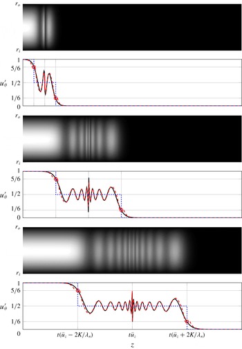
 $$\begin{eqnarray}\displaystyle u_{r}^{\prime }(z,r,t) & {\approx} & \displaystyle -0.5\mathop{\sum }_{n=1}^{\infty }\frac{c}{\sqrt{c^{2}\unicode[STIX]{x1D706}_{n}^{2}+4K^{2}}}\unicode[STIX]{x1D6FC}_{n}M_{1}(\unicode[STIX]{x1D706}_{n}r)\nonumber\\ \displaystyle & & \displaystyle \times \left[\unicode[STIX]{x1D6FF}\left(z-\frac{2Kct}{\sqrt{c^{2}\unicode[STIX]{x1D706}_{n}^{2}+4K^{2}}}\right)-\unicode[STIX]{x1D6FF}\left(z+\frac{2Kct}{\sqrt{c^{2}\unicode[STIX]{x1D706}_{n}^{2}+4K^{2}}}\right)\right],\end{eqnarray}$$
 $$\begin{eqnarray}\displaystyle u_{\unicode[STIX]{x1D703}}^{\prime }(z,r,t) & {\approx} & \displaystyle 0.5\mathop{\sum }_{n=1}^{\infty }\unicode[STIX]{x1D6FC}_{n}M_{1}(\unicode[STIX]{x1D706}_{n}r)\nonumber\\ \displaystyle & & \displaystyle \times \left[2-\text{H}\left(z-\frac{2Kct}{\sqrt{c^{2}\unicode[STIX]{x1D706}_{n}^{2}+4K^{2}}}\right)-\text{H}\left(z+\frac{2Kct}{\sqrt{c^{2}\unicode[STIX]{x1D706}_{n}^{2}+4K^{2}}}\right)\right],\qquad\end{eqnarray}$$
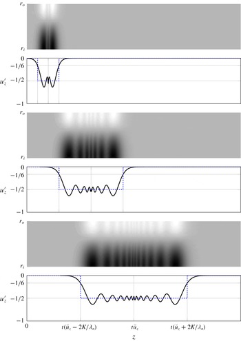
 $$\begin{eqnarray}\displaystyle u_{z}^{\prime }(z,r,t) & {\approx} & \displaystyle \unicode[STIX]{x1D700}_{a}\left[1-\text{H}(z-ct)\right]-0.5\mathop{\sum }_{n=1}^{\infty }\frac{\sqrt{c^{2}\unicode[STIX]{x1D706}_{n}^{2}+4K^{2}}}{c\unicode[STIX]{x1D706}_{n}}\unicode[STIX]{x1D6FC}_{n}M_{0}(\unicode[STIX]{x1D706}_{n}r)\nonumber\\ \displaystyle & & \displaystyle \times \left[\text{H}\left(z-\frac{2Kct}{\sqrt{c^{2}\unicode[STIX]{x1D706}_{n}^{2}+4K^{2}}}\right)-\text{H}\left(z+\frac{2Kct}{\sqrt{c^{2}\unicode[STIX]{x1D706}_{n}^{2}+4K^{2}}}\right)\right],\end{eqnarray}$$
 $$\begin{eqnarray}\displaystyle p^{\prime }(z,r,t) & {\approx} & \displaystyle \unicode[STIX]{x1D700}_{a}\bar{\unicode[STIX]{x1D70C}}c\left[1-\text{H}(z-ct)\right]-\bar{\unicode[STIX]{x1D70C}}K\mathop{\sum }_{n=1}^{\infty }\frac{\unicode[STIX]{x1D6FC}_{n}M_{0}(\unicode[STIX]{x1D706}_{n}r)}{\unicode[STIX]{x1D706}_{n}}\nonumber\\ \displaystyle & & \displaystyle \times \left[2-\text{H}\left(z-\frac{2Kct}{\sqrt{c^{2}\unicode[STIX]{x1D706}_{n}^{2}+4K^{2}}}\right)-\text{H}\left(z+\frac{2Kct}{\sqrt{c^{2}\unicode[STIX]{x1D706}_{n}^{2}+4K^{2}}}\right)\right].\qquad\end{eqnarray}$$
 $$\begin{eqnarray}\displaystyle \lim _{k\rightarrow 0}\unicode[STIX]{x1D714}_{n,i}=k\left(\bar{u}_{z}\pm \frac{2cK}{\sqrt{c^{2}\unicode[STIX]{x1D706}_{n}^{2}+4K^{2}}}\right). & & \displaystyle\end{eqnarray}$$
(This relation was also introduced as the low wavenumber limit of the group speed, see (2.29) in § 2.1.)
In most combustion applications, low Mach number flow is considered. At the same time, for thermo-acoustic applications, acoustic waves are also relevant. Therefore, an accurate and reasonable approximation is to keep the acoustic wave solution as it is and to neglect compressibility effects on inertial waves. This assumption further simplifies the solution to
 $$\begin{eqnarray}\displaystyle u_{r}^{\prime }(t,z,r) & {\approx} & \displaystyle -0.5\mathop{\sum }_{n=1}^{\infty }\frac{\unicode[STIX]{x1D6FC}_{n}M_{1}(\unicode[STIX]{x1D706}_{n}r)}{\unicode[STIX]{x1D706}_{n}}\nonumber\\ \displaystyle & & \displaystyle \times \left[\unicode[STIX]{x1D6FF}\left(z-\bar{u}_{z}t-\frac{2Kt}{\unicode[STIX]{x1D706}_{n}}\right)-\unicode[STIX]{x1D6FF}\left(z-\bar{u}_{z}t+\frac{2Kt}{\unicode[STIX]{x1D706}_{n}}\right)\right],\end{eqnarray}$$
 $$\begin{eqnarray}\displaystyle u_{\unicode[STIX]{x1D703}}^{\prime }(t,z,r) & {\approx} & \displaystyle 0.5\mathop{\sum }_{n=1}^{\infty }\unicode[STIX]{x1D6FC}_{n}M_{1}(\unicode[STIX]{x1D706}_{n}r)\nonumber\\ \displaystyle & & \displaystyle \times \left[2-\text{H}\left(z-\bar{u}_{z}t-\frac{2Kt}{\unicode[STIX]{x1D706}_{n}}\right)-\text{H}\left(z-\bar{u}_{z}t+\frac{2Kt}{\unicode[STIX]{x1D706}_{n}}\right)\right],\end{eqnarray}$$
 $$\begin{eqnarray}\displaystyle u_{z}^{\prime }(t,z,r) & {\approx} & \displaystyle \unicode[STIX]{x1D700}_{a}[1-\text{H}(z-\bar{u}_{z}t-ct)]+0.5\mathop{\sum }_{n=1}^{\infty }\unicode[STIX]{x1D6FC}_{n}M_{0}(\unicode[STIX]{x1D706}_{n}r)\nonumber\\ \displaystyle & & \displaystyle \times \left[\text{H}\left(z-\bar{u}_{z}t-\frac{2Kt}{\unicode[STIX]{x1D706}_{n}}\right)-\text{H}\left(z-\bar{u}_{z}t+\frac{2Kt}{\unicode[STIX]{x1D706}_{n}}\right)\right],\end{eqnarray}$$
 $$\begin{eqnarray}\displaystyle p^{\prime }(t,z,r) & {\approx} & \displaystyle \unicode[STIX]{x1D700}_{a}\bar{\unicode[STIX]{x1D70C}}c[1-\text{H}(z-\bar{u}_{z}t-ct)]-K\bar{\unicode[STIX]{x1D70C}}\mathop{\sum }_{n=1}^{\infty }\frac{\unicode[STIX]{x1D6FC}_{n}M_{0}(\unicode[STIX]{x1D706}_{n}r)}{\unicode[STIX]{x1D706}_{n}}\nonumber\\ \displaystyle & & \displaystyle \times \left[2-\text{H}\left(z-\bar{u}_{z}t-\frac{2Kt}{\unicode[STIX]{x1D706}_{n}}\right)-\text{H}\left(z-\bar{u}_{z}t+\frac{2Kt}{\unicode[STIX]{x1D706}_{n}}\right)\right].\end{eqnarray}$$
 $c\rightarrow \infty$
. There are two differences compared to the compressible solution. One is the inertial wave propagation speed, which is slightly faster in the incompressible case. This can be demonstrated by taking the incompressible limit for the propagation speed, i.e.
 $$\begin{eqnarray}\displaystyle \lim _{c\rightarrow \infty }\frac{2Kc}{\sqrt{c^{2}\unicode[STIX]{x1D706}_{n}^{2}+4K^{2}}}=\frac{2K}{\unicode[STIX]{x1D706}_{n}}. & & \displaystyle\end{eqnarray}$$
The other difference is that the inertial wave amplitude for axial velocity component,
 $u_{z}^{\prime }$
, decreases in the incompressible limit. Similarly, this can be shown by taking the limit for the amplitude as
 $$\begin{eqnarray}\displaystyle \lim _{c\rightarrow \infty }\frac{\sqrt{c^{2}\unicode[STIX]{x1D706}_{n}^{2}+4K^{2}}}{c\unicode[STIX]{x1D706}_{n}}=1. & & \displaystyle\end{eqnarray}$$
Note that these differences depend on Mach number and are therefore negligible for subsonic flows.
In terms of flame dynamics, the solution in (3.19) reveals the importance of inertial waves for flame front kinematics. Fleifil et al. (Reference Fleifil, Annaswamy, Ghoneim and Ghoniem1996) demonstrated that any flow perturbation normal to the flame surface disturbs the kinematic balance between flow and flame speeds and hence causes unsteady heat release rate. The flow perturbation due to plane acoustic waves at the flame front is one of the major contributions to thermo-acoustic instabilities and is investigated extensively in the literature (see Schuller, Durox & Candel (Reference Schuller, Durox and Candel2003), Blumenthal et al. (Reference Blumenthal, Subramanian, Sujith and Polifke2013) and Steinbacher et al. (Reference Steinbacher, Albayrak, Ghani and Polifke2019)). Similarly, axial and radial velocity perturbations resulting from inertial waves, respectively
 $u_{z}^{\prime }$
and
 $u_{r}^{\prime }$
in (3.19), play an important role in flame dynamics by modulating the flame surface. This is further discussed in the authors’ recent publication (Albayrak, Bezgin & Polifke Reference Albayrak, Bezgin and Polifke2018a
).
As discussed above, the time–space domain solution results from a simplified approach. The inertial wave dispersion effects are not present, but important properties such as propagation speeds and eigenmode structures are revealed. For comparison purposes, we also repeat the step response solution that results from the convective assumption for azimuthal velocity perturbations. This solution is equivalent to the solution proposed by Palies et al. (Reference Palies, Durox, Schuller and Candel2011a ) and is written as
 $$\begin{eqnarray}\displaystyle u_{r}^{\prime }(t,z,r) & = & \displaystyle 0,\end{eqnarray}$$
 $$\begin{eqnarray}\displaystyle u_{\unicode[STIX]{x1D703}}^{\prime }(t,z,r) & = & \displaystyle \unicode[STIX]{x1D700}_{a}\tan (\unicode[STIX]{x1D719})[1-\text{H}(z-\bar{u}_{z}t)],\end{eqnarray}$$
 $$\begin{eqnarray}\displaystyle u_{z}^{\prime }(t,z,r) & = & \displaystyle \unicode[STIX]{x1D700}_{a}[1-\text{H}(z-\bar{u}_{z}t)],\end{eqnarray}$$
 $$\begin{eqnarray}\displaystyle p^{\prime }(t,z,r) & = & \displaystyle \unicode[STIX]{x1D700}_{a}\bar{\unicode[STIX]{x1D70C}}c^{2}[1-\text{H}(z-\bar{u}_{z}t)].\end{eqnarray}$$
3.3.1 Asymptotic solution: method of steepest descent
In this section, we derive the asymptotic time–space domain solution by the method of steepest descent. For details of this method, the reader may consult Bender & Orszag (Reference Bender and Orszag1999). The asymptotic analysis here merely focuses on the incompressible inertial wave solution. Note that the same analysis can also be performed for the compressible case. However, as discussed in the previous section, plane acoustic waves are decoupled from the inertial wave solution at low Mach numbers. Moreover, the impact of compressibility on the inertial wave solution is negligible. This means that the analysis with compressible equations does not introduce additional aspects to the solution. In the incompressible limit, equation (3.16) reduces to
 $$\begin{eqnarray}\displaystyle \hat{u} _{r}(k,r,s) & = & \displaystyle -2Kk^{2}\left(\unicode[STIX]{x03C0}\unicode[STIX]{x1D6FF}(k)+\frac{\text{i}}{k}\right)\mathop{\sum }_{n=1}^{\infty }\frac{\unicode[STIX]{x1D6FC}_{n}M_{1}(\unicode[STIX]{x1D706}_{n}r)}{C^{2}(\unicode[STIX]{x1D706}_{n}^{2}+k^{2})-4K^{2}k^{2}},\end{eqnarray}$$
 $$\begin{eqnarray}\displaystyle \hat{u} _{\unicode[STIX]{x1D703}}(k,r,s) & = & \displaystyle \text{i}C\left(\unicode[STIX]{x03C0}\unicode[STIX]{x1D6FF}(k)+\frac{\text{i}}{k}\right)\mathop{\sum }_{n=1}^{\infty }\frac{(\unicode[STIX]{x1D706}_{n}^{2}+k^{2})\unicode[STIX]{x1D6FC}_{n}M_{1}(\unicode[STIX]{x1D706}_{n}r)}{C^{2}(\unicode[STIX]{x1D706}_{n}^{2}+k^{2})-4K^{2}k^{2}},\end{eqnarray}$$
 $$\begin{eqnarray}\displaystyle \hat{u} _{z}(k,r,s) & = & \displaystyle -2K\text{i}k\left(\unicode[STIX]{x03C0}\unicode[STIX]{x1D6FF}(k)+\frac{\text{i}}{k}\right)\mathop{\sum }_{n=1}^{\infty }\frac{\unicode[STIX]{x1D706}_{n}\unicode[STIX]{x1D6FC}_{n}M_{0}(\unicode[STIX]{x1D706}_{n}r)}{C^{2}(\unicode[STIX]{x1D706}_{n}^{2}+k^{2})-4K^{2}k^{2}},\end{eqnarray}$$
 $$\begin{eqnarray}\displaystyle \hat{p}(k,r,s) & = & \displaystyle -2K\text{i}C\bar{\unicode[STIX]{x1D70C}}\left(\unicode[STIX]{x03C0}\unicode[STIX]{x1D6FF}(k)+\frac{\text{i}}{k}\right)\mathop{\sum }_{n=1}^{\infty }\frac{\unicode[STIX]{x1D706}_{n}\unicode[STIX]{x1D6FC}_{n}M_{0}(\unicode[STIX]{x1D706}_{n}r)}{C^{2}(\unicode[STIX]{x1D706}_{n}^{2}+k^{2})-4K^{2}k^{2}}.\end{eqnarray}$$
 $$\begin{eqnarray}\displaystyle \hat{u} _{r}(k,r,t) & = & \displaystyle \frac{k}{2}\text{e}^{-\text{i}kt\bar{u}_{z}}\left(\unicode[STIX]{x03C0}\unicode[STIX]{x1D6FF}(k)+\frac{\text{i}}{k}\right)\mathop{\sum }_{n=1}^{\infty }\unicode[STIX]{x1D6FC}_{n}M_{1}(\unicode[STIX]{x1D706}_{n}r)\nonumber\\ \displaystyle & & \displaystyle \times \,\frac{\exp \left(-{\displaystyle \frac{2K\text{i}kt}{\sqrt{\unicode[STIX]{x1D706}_{n}^{2}+k^{2}}}}\right)-\exp \left({\displaystyle \frac{2K\text{i}kt}{\sqrt{\unicode[STIX]{x1D706}_{n}^{2}+k^{2}}}}\right)}{\sqrt{\unicode[STIX]{x1D706}_{n}^{2}+k^{2}}},\end{eqnarray}$$
 $$\begin{eqnarray}\displaystyle \hat{u} _{\unicode[STIX]{x1D703}}(k,r,t) & = & \displaystyle \frac{1}{2}\text{e}^{-\text{i}kt\bar{u}_{z}}\left(\unicode[STIX]{x03C0}\unicode[STIX]{x1D6FF}(k)+\frac{\text{i}}{k}\right)\mathop{\sum }_{n=1}^{\infty }\unicode[STIX]{x1D6FC}_{n}M_{1}(\unicode[STIX]{x1D706}_{n}r)\nonumber\\ \displaystyle & & \displaystyle \times \,\left[\exp \left(-{\displaystyle \frac{2K\text{i}kt}{\sqrt{\unicode[STIX]{x1D706}_{n}^{2}+k^{2}}}}\right)+\exp \left({\displaystyle \frac{2K\text{i}kt}{\sqrt{\unicode[STIX]{x1D706}_{n}^{2}+k^{2}}}}\right)\right],\end{eqnarray}$$
 $$\begin{eqnarray}\displaystyle \hat{u} _{z}(k,r,t) & = & \displaystyle \frac{\text{i}}{2}\text{e}^{-\text{i}kt\bar{u}_{z}}\left(\unicode[STIX]{x03C0}\unicode[STIX]{x1D6FF}(k)+\frac{\text{i}}{k}\right)\mathop{\sum }_{n=1}^{\infty }\unicode[STIX]{x1D706}_{n}\unicode[STIX]{x1D6FC}_{n}M_{0}(\unicode[STIX]{x1D706}_{n}r)\nonumber\\ \displaystyle & & \displaystyle \times \,\frac{\exp \left(-{\displaystyle \frac{2K\text{i}kt}{\sqrt{\unicode[STIX]{x1D706}_{n}^{2}+k^{2}}}}\right)-\exp \left({\displaystyle \frac{2K\text{i}kt}{\sqrt{\unicode[STIX]{x1D706}_{n}^{2}+k^{2}}}}\right)}{\sqrt{\unicode[STIX]{x1D706}_{n}^{2}+k^{2}}},\end{eqnarray}$$
 $$\begin{eqnarray}\displaystyle \hat{p}(k,r,t) & = & \displaystyle -K\bar{\unicode[STIX]{x1D70C}}\text{e}^{-\text{i}kt\bar{u}_{z}}\left(\unicode[STIX]{x03C0}\unicode[STIX]{x1D6FF}(k)+\frac{\text{i}}{k}\right)\mathop{\sum }_{n=1}^{\infty }\unicode[STIX]{x1D706}_{n}\unicode[STIX]{x1D6FC}_{n}M_{0}(\unicode[STIX]{x1D706}_{n}r)\nonumber\\ \displaystyle & & \displaystyle \times \,\frac{\exp \left(-{\displaystyle \frac{2K\text{i}kt}{\sqrt{\unicode[STIX]{x1D706}_{n}^{2}+k^{2}}}}\right)+\exp \left({\displaystyle \frac{2K\text{i}kt}{\sqrt{\unicode[STIX]{x1D706}_{n}^{2}+k^{2}}}}\right)}{\unicode[STIX]{x1D706}_{n}^{2}+k^{2}}.\end{eqnarray}$$
 $\text{e}^{-\text{i}kt\bar{u}_{z}}$
. The inertial wave propagation is governed by exponential functions inside the summation, where fast and slow propagating waves are indicated by the negative and positive sign in the exponential function, respectively. The denominator of the exponential function,
 $\sqrt{\unicode[STIX]{x1D706}_{n}^{2}+k^{2}}$
, is the reason for the dispersive propagation. At this point, no closed form solution for the inverse Fourier transform exists. Similar to the previous section, one can seek the solution at low wavenumbers, i.e.
 $k\rightarrow 0$
. This leads exactly to the inertial wave solution as described in (3.19). Instead, we continue with the method of steepest descent. Here, for simplicity only the fast propagating solution of the azimuthal velocity
 $\hat{u} _{\unicode[STIX]{x1D703}}$
is presented. Other components may be derived in a similar manner. Moreover, only the
 $n$
th mode is considered, so that the summation is not required. The convection process is neglected and terms that do not depend on
 $k$
are not included. However, in the final expression, equation (3.28), the most general form of the solution is presented. Under these conditions, the integral for the inverse Fourier transformation is written
 $$\begin{eqnarray}\displaystyle I(z)=\int _{-\infty }^{\infty }f(k)\text{e}^{zg(k)}=\int _{-\infty }^{\infty }\left(\unicode[STIX]{x03C0}\unicode[STIX]{x1D6FF}(k)+\frac{\text{i}}{k}\right)\exp \left(z\left[\text{i}k-{\displaystyle \frac{2\text{i}Kk}{\unicode[STIX]{x1D702}\sqrt{\unicode[STIX]{x1D706}_{n}^{2}+k^{2}}}}\right]\right)\,\text{d}k, & & \displaystyle\end{eqnarray}$$
where
 $\unicode[STIX]{x1D702}=z/t$
. Real and imaginary parts of the exponent function,
 $g(k)$
, are shown in figure 6 as contour plots. Columns correspond to the real and imaginary parts, respectively. Darker colours indicate lower values. The singularities are marked with red circles at
 $k=\pm \unicode[STIX]{x1D706}_{n}$
. Corresponding branch cuts are on the imaginary axis, i.e.
 $k>\text{i}\unicode[STIX]{x1D706}_{n}$
and
 $k<-\text{i}\unicode[STIX]{x1D706}_{n}$
. Dashed blue contours indicate constant levels of imaginary part,
 $\text{Im}(g(k))$
.
Contour plots of real (a) and imaginary (b) parts of
 $g(k)$
. From (a–f), three branches are plotted,
 $\unicode[STIX]{x1D702}>2K/\unicode[STIX]{x1D706}_{n}$
,
 $\unicode[STIX]{x1D702}=2K/\unicode[STIX]{x1D706}_{n}$
and
 $\unicode[STIX]{x1D702}<2K/\unicode[STIX]{x1D706}_{n}$
. Circles and crosses indicate poles of
 $g(k)$
and zeros of
 $g^{\prime }(k)$
, respectively. Dashed blue and solid green (with arrows) lines indicate constant levels of contours and closed integral paths for the steepest descent path, respectively.

Saddle points,
 $\unicode[STIX]{x2202}g/\unicode[STIX]{x2202}k|_{k=k_{0}}=0$
, are determined as
 $$\begin{eqnarray}\displaystyle k_{0}=\pm \unicode[STIX]{x1D706}_{n}\sqrt{\left(\frac{2K}{\unicode[STIX]{x1D702}\unicode[STIX]{x1D706}_{n}}\right)^{2/3}-1}. & & \displaystyle\end{eqnarray}$$
Observing the form of saddle points, three different branches are recognized as
 $\unicode[STIX]{x1D702}>2K/\unicode[STIX]{x1D706}_{n}$
,
 $\unicode[STIX]{x1D702}=2K/\unicode[STIX]{x1D706}_{n}$
and
 $\unicode[STIX]{x1D702}<2K/\unicode[STIX]{x1D706}_{n}$
. The first branch is shown in figure 6(a,b). Two non-degenerate saddle points marked with red crosses are located on the imaginary axis. Similarly, there exists two saddle points for the branch,
 $\unicode[STIX]{x1D702}<2K/\unicode[STIX]{x1D706}_{n}$
, which is shown in the last row. The saddle points lie on the real axis. For
 $\unicode[STIX]{x1D702}=2K/\unicode[STIX]{x1D706}_{n}$
, there exist a single degenerate saddle point at the origin.
For each branch, the initial integral path,
 $k=(-\infty ,\infty )$
is constructed by additional paths from the steepest descent method. Cauchy’s integral theorem is employed, which states that the integral along a closed path with no singularities is zero. The closed integral paths are indicated with the green colour (solid lines with arrows). As an example, only the first branch is discussed in detail. The closed integral path is written
 $$\begin{eqnarray}\displaystyle \underbrace{\int _{\unicode[STIX]{x1D6E4}_{1}}+\int _{\unicode[STIX]{x1D6E4}_{2}}}_{I(z)}+\underbrace{\int _{\unicode[STIX]{x1D6E4}_{3}}+\int _{\unicode[STIX]{x1D6E4}_{6}}}_{C(z)}+\underbrace{\int _{\unicode[STIX]{x1D6E4}_{4}}+\int _{\unicode[STIX]{x1D6E4}_{5}}}_{S(z)}=0, & & \displaystyle\end{eqnarray}$$
where
 $S(z)$
is the contribution by steepest descent path, which follows the constant level of
 $\text{Im}(g(k))$
. Note that the saddle point in the negative imaginary axis is a local minimum and does not define a steepest descent path. Thus, only the saddle point in the positive imaginary axis is employed. The circular paths,
 $C(z)$
, enclose the contour so that Cauchy’s integral theorem can be employed. As the radius of the circular path grows to infinity, its contribution vanishes,
 $C(z)=0$
. Hence, the integral,
 $I(z)$
, can be related to the steepest descent integral,
 $I(z)=-S(z)$
. Similar arguments apply for the other two branches of
 $\unicode[STIX]{x1D702}$
. The leading term for steepest descent integral results in the general expression for azimuthal velocity perturbations as
 $$\begin{eqnarray}\displaystyle & & \displaystyle \hspace{-35.00005pt}u_{\unicode[STIX]{x1D703}}^{\prime }(t,z,r)\approx \mathop{\sum }_{n=1}^{\infty }\unicode[STIX]{x1D6FC}_{n}M_{r,n}\nonumber\\ \displaystyle & & \displaystyle \hspace{-35.00005pt}\quad \times \,\left\{\begin{array}{@{}ll@{}}\displaystyle 1-\left(\frac{2Kt}{\unicode[STIX]{x1D706}_{n}(\bar{u}_{z}t-z)}\right)^{1/3}\frac{\exp (-\unicode[STIX]{x1D706}_{n}(-c_{m})^{3/2})}{2\sqrt{6\unicode[STIX]{x03C0}\unicode[STIX]{x1D706}_{n}}(-c_{m})^{3/4}}\quad & \text{if }\displaystyle \unicode[STIX]{x1D702}<\bar{u}_{z}-\frac{2K}{\unicode[STIX]{x1D706}_{n}},\\ \displaystyle \frac{5}{6}\quad & \text{if }\displaystyle \unicode[STIX]{x1D702}=\bar{u}_{z}-\frac{2K}{\unicode[STIX]{x1D706}_{n}},\\ \displaystyle \frac{1}{2}+\left(\frac{2Kt}{\unicode[STIX]{x1D706}_{n}(\bar{u}_{z}t-z)}\right)^{1/3}\frac{\cos (\unicode[STIX]{x1D706}_{n}c_{m}^{3/2})-\sin (\unicode[STIX]{x1D706}_{n}c_{m}^{3/2})}{2\sqrt{3\unicode[STIX]{x03C0}\unicode[STIX]{x1D706}_{n}}c_{m}^{3/4}}\quad & \text{if }\displaystyle \bar{u}_{z}-\frac{2K}{\unicode[STIX]{x1D706}_{n}}<\unicode[STIX]{x1D702}<\bar{u}_{z},\\ \displaystyle \frac{1}{2}-\left(\frac{2Kt}{\unicode[STIX]{x1D706}_{n}(z-\bar{u}_{z}t)}\right)^{1/3}\frac{\cos (\unicode[STIX]{x1D706}_{n}c_{p}^{3/2})-\sin (\unicode[STIX]{x1D706}_{n}c_{p}^{3/2})}{2\sqrt{3\unicode[STIX]{x03C0}\unicode[STIX]{x1D706}_{n}}c_{p}^{3/4}}\quad & \text{if }\displaystyle \bar{u}_{z}<\unicode[STIX]{x1D702}<\bar{u}_{z}+\frac{2K}{\unicode[STIX]{x1D706}_{n}},\\ \displaystyle \frac{1}{6}\quad & \text{if }\displaystyle \unicode[STIX]{x1D702}=\bar{u}_{z}+\frac{2K}{\unicode[STIX]{x1D706}_{n}},\\ \displaystyle \left(\frac{2Kt}{\unicode[STIX]{x1D706}_{n}(z-\bar{u}_{z}t)}\right)^{1/3}\frac{\exp (-\unicode[STIX]{x1D706}_{n}(-c_{m})^{3/2})}{2\sqrt{6\unicode[STIX]{x03C0}\unicode[STIX]{x1D706}_{n}}(-c_{m})^{3/4}}\quad & \text{if }\displaystyle \unicode[STIX]{x1D702}>\bar{u}_{z}+\frac{2K}{\unicode[STIX]{x1D706}_{n}},\end{array}\right.\end{eqnarray}$$
where
 $$\begin{eqnarray}\displaystyle c_{p} & = & \displaystyle \left(\frac{2Kt}{\unicode[STIX]{x1D706}_{n}}\right)^{2/3}-(z-\bar{u}_{z}t)^{2/3},\end{eqnarray}$$
 $$\begin{eqnarray}\displaystyle c_{m} & = & \displaystyle \left(\frac{2Kt}{\unicode[STIX]{x1D706}_{n}}\right)^{2/3}-(\bar{u}_{z}t-z)^{2/3}.\end{eqnarray}$$
In figure 7, three snapshots of the spatio-temporal development of azimuthal velocity fluctuations after a step perturbation are presented. The colour raster plots show velocity values ranging from 0 (black) to 1 (white) in the
 $z$
–
 $r$
plane, i.e. the annulus between inner radius
 $r_{i}$
and outer radius
 $r_{o}$
. For simplicity, only the first mode
 $n=1$
with a radial profile corresponding to the first eigenmode of azimuthal velocity
 $M_{1}(\unicode[STIX]{x1D706}_{1}r)$
is presented here. Corresponding results for other modes or multiple modes can be generated without difficulty. Below each surface plot, axial profiles of perturbation amplitude are shown. Solid black lines indicate the numerical inverse fast Fourier transformation of (3.24). Dotted blue lines indicate the simplified non-dispersive solution (see (3.19)) developed in the previous section. Dashed red lines indicate the asymptotic solution in (3.28). By inspecting this equation, the solution can be divided into regions: The first region,
 $\unicode[STIX]{x1D702}<\bar{u}_{z}-2K/\unicode[STIX]{x1D706}_{n}$
, converges exponentially to 1. For the non-dispersive solution, this region is estimated as 1 without an exponential term. Similarly, the last region,
 $\unicode[STIX]{x1D702}>\bar{u}_{z}-2K/\unicode[STIX]{x1D706}_{n}$
, decays exponentially to 0. Again, the non-dispersive solution estimates only a constant value of 0. The second region and third regions,
 $\bar{u}_{z}-2K/\unicode[STIX]{x1D706}_{n}>\unicode[STIX]{x1D702}>\bar{u}_{z}+2K/\unicode[STIX]{x1D706}_{n}$
, correspond to the dispersive region of inertial propagation, where oscillations around
 $0.5$
are observed. The asymptotic solution captures the oscillations accurately via the combination of trigonometric functions. Like a chirp function, oscillations become squeezed as they approach the convective line
 $\unicode[STIX]{x1D702}=\bar{u}_{z}$
. In other works, near the convective region, high axial wavenumbers are observed. This is also confirmed in figure 3, where the group speed is shown as a function of the axial wavenumber. As the axial wavenumber increases, the propagation of inertial waves converges to the convection speed. The non-dispersive solution, as its name suggests, cannot capture these oscillations and estimates a constant value of 0.5. Note that the asymptotic solution diverges close to the boundaries
 $\unicode[STIX]{x1D702}=\bar{u}_{z}-2K/\unicode[STIX]{x1D706}_{n}$
and
 $\unicode[STIX]{x1D702}=\bar{u}_{z}+2K/\unicode[STIX]{x1D706}_{n}$
, since saddle points move in the complex plane abruptly (see regions in figure 6). Exactly at these boundaries, the asymptotic solution yields
 $5/6$
and
 $1/6$
, respectively. These points are indicated in figure 7 by circles. The non-dispersive solution estimates step changes at these locations.
Three snapshots of the azimuthal velocity fluctuation field developing after a step perturbation by a downstream propagating acoustic wave. Only the first eigenmode is considered, thus the radial profile
 $u_{\unicode[STIX]{x1D703}}^{\prime }(r)\propto M_{1}(\unicode[STIX]{x1D706}_{n}r)$
. Colour raster plots were generated via the inverse fast Fourier transformation of (3.24). Axial profile plots compare that solution (solid black line) with the non-dispersive solution (3.19) (dotted blue line) and the asymptotic solution (3.28) obtained with the steepest descent method (dashed red line).

Three snapshots of the axial velocity fluctuation field developing after a step perturbation by a downstream propagating acoustic wave. Only the first eigenmode is considered, thus the radial profile
 $u_{z}^{\prime }(r)\propto M_{0}(\unicode[STIX]{x1D706}_{n}r)$
. Colour raster plots were generated via the inverse fast Fourier transformation. Axial profile plots compare that solution (solid black line) with the non-dispersive solution (3.19) (dotted blue line).

Three snapshots of the radial velocity fluctuation field developing after a step perturbation by a downstream propagating acoustic wave. Only the first eigenmode with radial profile
 $u_{r}^{\prime }(r)\propto M_{1}(\unicode[STIX]{x1D706}_{n}r)$
is considered. Colour raster plots were generated via the inverse fast Fourier transformation. Axial profile plots compare that solution (black line) with the non-dispersive solution (3.19) (blue line). Note that the Dirac delta function is represented by the circles at
 $\pm 0.5$
.

Three snapshots of the pressure fluctuation field developing after a step perturbation by a downstream propagating acoustic wave. Only the first eigenmode radial profile
 $p^{\prime }(r)\propto M_{0}(\unicode[STIX]{x1D706}_{n}r)$
is considered. Colour raster plots were generated via the inverse fast Fourier transformation. Axial profile plots compare that solution (solid black line) with the non-dispersive solution (3.19) (dotted blue line).

The other components of the fluctuation field are shown in subsequent figures. Figure 8 presents axial velocity. Perturbations decay to zero for both the first and the last regions. This means that the axial velocity perturbations are constrained to the second and third region, where dispersive oscillations around the value of
 $-0.5$
are present. The non-dispersive solution estimates a constant value of
 $-0.5$
for the oscillatory region. The mode shape corresponds to
 $M_{0}(\unicode[STIX]{x1D706}_{1}r)$
.
In figure 9 the radial velocity fluctuation is shown. No step changes are observed, and the solution oscillates around zero for the second and third region. Note that the non-dispersive solution estimates only Dirac delta functions for at
 $\unicode[STIX]{x1D702}=\bar{u}_{z}-2K/\unicode[STIX]{x1D706}_{n}$
and
 $\unicode[STIX]{x1D702}=\bar{u}_{z}+2K/\unicode[STIX]{x1D706}_{n}$
, indicated at
 $\pm 0.5$
by blue circles.
Figure 10 presents pressure fluctuations, normalized by
 $2\bar{\unicode[STIX]{x1D70C}}K$
. An analogous argument to that for the azimuthal velocity applies but the amplitude is negative, i.e. the first region converges to
 $-1$
. As discussed previously, the initial perturbation in pressure does not show up as an initial condition for the incompressible equations due to the elliptic continuity equation. However, the initial azimuthal velocity perturbation induces also pressure fluctuations as seen in the solution due to the Coriolis force in the radial momentum balance. Although it does not play a role in the incompressible equations, it should be included for the compressible equations because they show up in the equations as an initial condition. Therefore, this term is introduced in the actuator disk theory (see (3.11)) for the consistency of inertial waves.
4 Inertial wave propagation speed in a premix swirl burner
In this section, we revisit the premix swirl burner investigated by Komarek & Polifke (Reference Komarek and Polifke2010). The principal objectives of that study were to make explicit the effects of superposition of flame responses to axial and azimuthal velocity perturbations, respectively, on the overall transfer function of a swirl flame. Thus the burner was designed such that the distance between the axial swirler and the burner exit could be easily varied by approximately half a convective wavelength. With such a configuration it was possible to alternate between constructive and destructive superposition of the respective contributions to the swirl flame dynamics, and indeed it was observed that both the gain and phase of the flame transfer function depend in a very sensitive manner on the position of the swirl generator (while the mean flame shape was almost unaffected).
The experimental results were corroborated by numerical simulation and supplemented with low-order models based on distributed time delays for the respective flame responses to axial and azimuthal velocity perturbations. An important parameter in the sub-model for the response to azimuthal velocity perturbations is the time required for propagation from the swirler to the root of the flame, which should depend on the ratio of the distance between swirler and burner exit, and the velocity of propagation. Komarek & Polifke (Reference Komarek and Polifke2010) reported that a match between the model for the flame transfer function and experiment was achieved if that velocity was set to a value that exceeds the bulk velocity in the burner by approximately 40 %. This observation, which suggested that propagation of azimuthal velocity fluctuations was not strictly convective, was subsequently confirmed in follow-up studies (Palies et al. Reference Palies, Durox, Schuller and Candel2011b ; Acharya & Lieuwen Reference Acharya and Lieuwen2014) and motivated the present work.
With the results of the present study, the speed of propagation of azimuthal velocity fluctuations can be estimated in a simple manner: we only consider the first inertial wave mode in the limit of low axial wavenumber resulting from (2.28). For cases where more detailed experimental data are available, or where the flow physics is more complicated, a more sophisticated treatment based on (3.28) might be necessary.
For the case considered with power rating 30 kW, the Reynolds number in the annular duct with inner and outer radii of
 $r_{i}=8$
mm and
 $r_{o}=20$
mm is
 $Re=18\,000$
, with corresponding bulk velocity
 $\bar{u}_{z}=11.3~\text{m}~\text{s}^{-1}$
. Following Kerrebrock (Reference Kerrebrock1977), we assume that the azimuthal velocity profile downstream of the swirler quickly develops towards stable solid body rotation. For a design point swirl angle
 $\unicode[STIX]{x1D719}=45^{\circ }$
, this redistribution of azimuthal momentum
 $$\begin{eqnarray}\displaystyle \int _{r_{i}}^{r_{o}}2\unicode[STIX]{x03C0}r\bar{u}_{z}\tan (\unicode[STIX]{x1D719})\,\text{d}r\rightarrow \int _{r_{i}}^{r_{o}}2\unicode[STIX]{x03C0}rKr\,\text{d}r & & \displaystyle\end{eqnarray}$$
implies a design point circulation strength
 $K=760~\text{s}^{-1}$
. We proceed with the first inertial wave mode
 $n=1$
, as according to the discussion in § 2.4 it is the least damped eigenmode. By employing the boundary condition for eigenmodes (2.13), the first eigenvalue is computed as
 $\unicode[STIX]{x1D706}_{1}=270~\text{m}^{-1}$
. The highest deviation in the propagation speed is observed in the limit of low axial wavenumber. The relative deviation in inertial wave propagation speed from bulk velocity is computed from the group speed at this limit (see (2.28)),
 $$\begin{eqnarray}\displaystyle \frac{2K/\unicode[STIX]{x1D706}_{1}}{\bar{u}_{z}}\times 100\approx 50\,\%. & & \displaystyle\end{eqnarray}$$
Komarek & Polifke (Reference Komarek and Polifke2010) employed a propagation speed model, which is approximately 40 % above the convection speed. Given the fact that this deviation is obtained from a quite simplistic flame response model parameter ‘time lag’ to match experimental results, the agreement with our analysis is indeed very satisfactory. Obviously, application of this analysis to other configurations is straightforward, provided that duct dimensions, bulk velocity and swirl angle are known.
5 Summary and conclusions
The propagation of azimuthal velocity perturbations downstream of a swirl generator is an important factor for the dynamic response of swirl flames to acoustic perturbations and their thermo-acoustic stability. It has been reported repeatedly that the velocity of propagation of such perturbations exceeds the speed of convection by 40 %–50 % (Komarek & Polifke Reference Komarek and Polifke2010; Palies et al. Reference Palies, Durox, Schuller and Candel2011b ; Acharya & Lieuwen Reference Acharya and Lieuwen2014). A fundamental, physics-based justification of this deviation has not been proposed until now, and it was not possible to predict the propagation speed as a function of mean flow parameters.
This study argues that azimuthal velocity perturbations generated across a swirler are not simply convected by the mean flow, but instead should be regarded as inertial waves, which propagate at speeds governed by a non-trivial dispersion relation. This dispersion relation was obtained by considering inertial wave solutions of the linearized Euler equations. It was found that the dispersive behaviour of the inertial waves generates two families of waves, one propagating faster and the other slower than the speed of convection. The latter family has not been observed or discussed previously.
In order to describe the spatio-temporal evolution of inertial waves downstream of a swirl generator that is exposed to incident, plane acoustic waves, an initial value problem was formulated by imposing a sudden increase of azimuthal velocity on the downstream side of the swirler. The corresponding step response solution was derived firstly in the limit of low wavenumber. Both compressible and incompressible cases were discussed. These simplified solutions were found to be non-dispersive. A more rigorous asymptotic solution was developed by employing the method of steepest descent.
The results of the present analysis compare favourably with the experimental observations of Komarek & Polifke (Reference Komarek and Polifke2010), and we conclude that inertial wave propagation can account for the reported differences between the speeds of convection and propagation of azimuthal velocity fluctuations. The proposed solution also describes the dependency of the deviation on the circulation strength, i.e. the observation that with increasing circulation propagation speeds deviate more strongly. This behaviour can be approximated by a concise analytical expression for the convection speed, derived from modal decomposition of the linearized Euler equations as an initial value problem. The result can be incorporated into reduced-order models of thermo-acoustic systems in order to model this effect.
Since the seminal paper of Richards & Yip (Reference Richards and Yip1995), the exact mechanism by which fluctuations of azimuthal velocity modulate the rate of heat release by the flame has been a matter of debate. As discussed in the introduction, several authors have endeavoured to identify the governing flow–flame interaction mechanisms and to quantify the flame response to swirl fluctuations. The present paper makes an important contribution to this discussion, because it characterizes not only the propagation speed, but also the structure of inertial waves. In particular, the eigenmode analysis shows that inertial waves comprise velocity perturbations in all directions. The perturbations in the axial and radial directions can perturb directly the kinematic balance at the flame front and thus modify the position, shape, surface area and heat release rate of the flame. These effects were explored by Albayrak et al. (Reference Albayrak, Bezgin and Polifke2018a ) in a first attempt to model analytically the response of a laminar swirl flame to inertial waves.
Acknowledgements
We are indebted to the second anonymous reviewer of the draft version of this paper. Following the reviewer’s suggestion, we employed the method of steepest descent for the derivation of the time–space domain solution. We acknowledge financial support for A.A. from the European Commission in the framework of the Marie Curie Initial Training Network Thermo-acoustic and aero-acoustic nonlinearities in green combustors with orifice structures (TANGO) under call FP7-PEOPLE-ITN-2012. We are grateful to the anonymous reviewer, who made us aware of the paper by Renac et al. (Reference Renac, Sipp and Jacquin2007).