1 Introduction
In observations and numerical simulations, the strongest submesoscale currents in the upper ocean are often horizontal jets, fronts, filaments and vortices with horizontal scales from tens of metres to tens of kilometres (McWilliams Reference McWilliams2016). These currents are approximately in geostrophic, hydrostatic balance with the sea level, pressure and buoyancy fields. All of these flow configurations are ‘coherent structures’ that are in dynamically preferred states – i.e. attractors with respect to the nonlinear advective dynamics – with a relatively slow evolution rate
 $t_{cs}^{-1}$
compared to a canonical turbulent decorrelation eddy-turnover rate for a more disordered flow configuration with comparable scales, i.e.
 $t_{eddy}^{-1}=V_{g}/\ell$
, where
 $\ell$
is the cross-flow horizontal length scale and
 $V_{g}$
is the geostrophic velocity scale. For example, in a vortex
 $\ell$
is the radial scale, and
 $V_{g}$
is the azimuthal velocity; in a front or filament
 $\ell$
is the cross-axis scale, and
 $V_{g}$
is the along-axis velocity. In the submesoscale regime, the Rossby number (
 $Ro=V_{g}/f\ell$
, where
 $f$
is the local Coriolis frequency) is usually not small, but neither is it so large as to make rotational effects unimportant.
Associated with the geostrophic currents are ageostrophic secondary circulations and surface boundary-layer turbulence. Often the horizontal buoyancy and velocity horizontal gradients sharpen in frontogenesis, which gives rise to the prevalent frontal and filamentary structures. In McWilliams (Reference McWilliams2017) (denoted by SF1), a diagnostic framework is adduced for analysing the secondary circulation and frontogenetic tendency (i.e. SCFT for short) and the buoyancy flux for fronts and filaments in the presence of wind stress and turbulent vertical momentum mixing. A balanced approximation is made by neglecting ageostrophic acceleration. This situation is called the turbulent thermal-wind (TTW) balance, including its generalization to include advective nonlinearity at finite
 $Ro$
. Furthermore, the more familiar conception of frontogenesis caused by an ambient horizontal strain flow (Hoskins Reference Hoskins1982) is also analysed in SF1 for comparison with TTW.
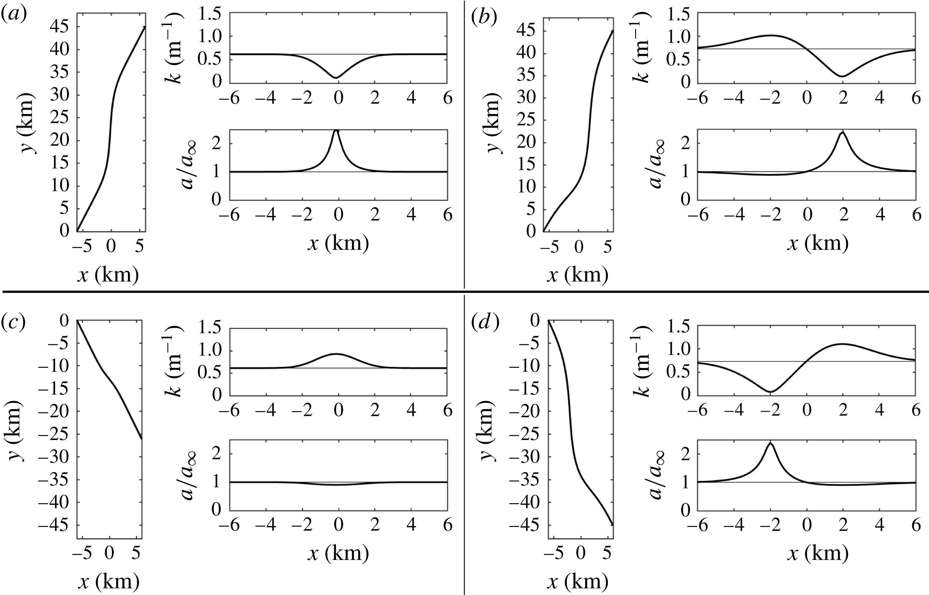
Surface gravity waves have important influences on near-surface and/or near-shore currents, often referred to as wave effects on currents (WEC), which are the subject of this paper. Beyond the wave orbital motion, whose Eulerian mean is approximately zero, the WEC influences are primarily through wave breaking (i.e. a transmission of wave momentum to the currents) and through the Lagrangian mean current, the Stokes drift. In an oceanic circulation model, wave breaking is often subsumed in the surface wind-stress representation except for the depth-induced breaking in the surf zone; however, the Stokes-drift effects require additional wave-averaged forces and material advection terms (§ 2.1) that emerge from multi-scale asymptotic theories (Craik & Leibovich Reference Craik and Leibovich1976; Holm Reference Holm1996; McWilliams, Restrepo & Lane Reference McWilliams, Restrepo and Lane2004). Surface waves exhibit great variety in nature, but an important concept is wind–wave equilibrium (WWE) where statistically steady winds generate an equilibrium spectrum of local wind waves, distinct from remotely generated swell. In WWE, the momentum and energy lost from the wind are locally equal to those transmitted to the currents (including upper-ocean turbulence) through wave breaking, WEC and diffusion.
The problem of Langmuir turbulence (i.e. the turbulent surface boundary layer under the influence of surface gravity waves) has been studied extensively (e.g. the review in Sullivan & McWilliams Reference Sullivan and McWilliams2010), but the interaction between surface waves and submesoscale currents has had relatively little attention (but see McWilliams & Fox-Kemper Reference McWilliams and Fox-Kemper2013). In this paper the SCFT methodology is extended to include WEC as expressed in wave-averaged equations for the current dynamics in the presence of a specified wave field and its associated Stokes drift. Then representative diagnostic solutions are analysed. Because of the similarities between both the methodology and the SCFT results, many shortcuts will be taken here by referencing SF1. In § 2 the generalized SCFT model is presented, and in § 3 specific problems for two-dimensional (2-D) fronts and filaments are posed. In § 4 a TTW SCFT solution is recalled for comparison with the new WEC results that are presented in § 5. A brief analysis of current effects on waves (CEW) near submesoscale fronts and filaments is made in § 6. Section 7 is a summary and final discussion.
2 Dynamical model
2.1 Conservative wave-averaged effects
In a multi-scale asymptotic theory for surface wave–current interaction, the wave-averaged dynamical equations for the currents and their material tracers contain additional terms due to the presence of waves. In the momentum balance the combined Stokes Coriolis and Stokes vortex force is
 $$\begin{eqnarray}\displaystyle \boldsymbol{u}_{st\,3}\times (f\hat{\boldsymbol{z}}_{3}+\unicode[STIX]{x1D73B}_{3}), & & \displaystyle\end{eqnarray}$$
where
 $\boldsymbol{u}_{3}$
is the velocity vector,
 $\boldsymbol{u}_{st\,3}$
is the Stokes drift,
 $\unicode[STIX]{x1D73B}_{3}=\unicode[STIX]{x1D735}_{3}\times \boldsymbol{u}_{3}$
is the vorticity vector and the traditional Coriolis force approximation is made with only the component of Earth’s rotation vector in the local vertical direction
 $\hat{\boldsymbol{z}}_{3}$
. Three-dimensional vectors in bold face are denoted by the subscript 3; 2-D vectors are boldface without this subscript. The Stokes-drift material advection acting as a buoyancy tendency is
 $$\begin{eqnarray}\displaystyle -\boldsymbol{u}_{st\,3}\boldsymbol{\cdot }\unicode[STIX]{x1D735}_{3}b, & & \displaystyle\end{eqnarray}$$
where
 $b=-g(\unicode[STIX]{x1D70C}/\unicode[STIX]{x1D70C}_{0}-1)$
with
 $g$
the gravitational acceleration,
 $rho$
the density and
 $\unicode[STIX]{x1D70C}_{0}$
a constant average value. In addition there are extra wave-averaged terms included in the pressure-gradient force,
 $-\unicode[STIX]{x1D735}_{3}\unicode[STIX]{x1D719}$
, and in the free-surface boundary conditions (Holm Reference Holm1996; McWilliams et al.
Reference McWilliams, Restrepo and Lane2004) that need not be made explicit here in solving the incompressible primitive equations with a rigid-lid approximation (§ 2.2).
In this paper
 $\boldsymbol{u}_{st\,3}$
will be assumed to depend only on
 $z$
, hence its vertical component
 $w_{st}$
is zero. (This will briefly be reconsidered in § 6.)
2.2 Primitive equations
Assume there is a background stratified resting state that depends only on
 $z$
. Decompose the full pressure and buoyancy fields into mean and deviation components, and assume hydrostatic balance for the background (implicitly including added wave terms that also depend only on
 $z$
):
 $$\begin{eqnarray}\displaystyle \unicode[STIX]{x1D719}=\overline{\unicode[STIX]{x1D719}}+\unicode[STIX]{x1D719}^{\prime },\quad b=\overline{b}+b^{\prime },\quad \unicode[STIX]{x2202}_{z}\overline{\unicode[STIX]{x1D719}}=\overline{b}. & & \displaystyle\end{eqnarray}$$
The background buoyancy frequency is
 $N^{2}(z)=\unicode[STIX]{x2202}_{z}\overline{b}$
.
The hydrostatic primitive equations for the deviation fields with vertical mixing and the conservative wave-averaged effects (2.1), (2.2) are the following:
 $$\begin{eqnarray}\displaystyle \left.\begin{array}{@{}c@{}}\displaystyle D[u]-f(y)v=-\unicode[STIX]{x2202}_{x}\unicode[STIX]{x1D719}^{\prime }+v_{st}(f(y)+\unicode[STIX]{x1D701}^{z})+\unicode[STIX]{x2202}_{z}[\unicode[STIX]{x1D708}_{v}\unicode[STIX]{x2202}_{z}u],\\ \displaystyle D[v]+f(y)u=-\unicode[STIX]{x2202}_{y}\unicode[STIX]{x1D719}^{\prime }-u_{st}(f(y)+\unicode[STIX]{x1D701}^{z})+\unicode[STIX]{x2202}_{z}[\unicode[STIX]{x1D708}_{v}\unicode[STIX]{x2202}_{z}v],\\ \displaystyle \unicode[STIX]{x2202}_{z}\unicode[STIX]{x1D719}^{\prime }=b^{\prime }+u_{st}(\unicode[STIX]{x2202}_{z}u-\unicode[STIX]{x2202}_{x}w)+v_{st}(\unicode[STIX]{x2202}_{z}v-\unicode[STIX]{x2202}_{y}w),\\ \displaystyle D[b]^{\prime }=-\boldsymbol{u}_{st}\boldsymbol{\cdot }\unicode[STIX]{x1D735}b^{\prime }+\unicode[STIX]{x2202}_{z}[\unicode[STIX]{x1D705}_{v}\unicode[STIX]{x2202}_{z}b]^{\prime },\\ \displaystyle \unicode[STIX]{x1D735}\boldsymbol{\cdot }\boldsymbol{u}+\unicode[STIX]{x2202}_{z}w=0.\end{array}\right\} & & \displaystyle\end{eqnarray}$$
The 3-D coordinate and velocity vectors are
 $\boldsymbol{x}_{3}=(x,y,z)$
and
 $\boldsymbol{u}_{3}=(u,v,w)$
.
 $\unicode[STIX]{x1D701}^{z}=\unicode[STIX]{x2202}_{x}v-\unicode[STIX]{x2202}_{y}u$
is the vertical vorticity.
 $D=\unicode[STIX]{x2202}_{t}+\boldsymbol{u}\boldsymbol{\cdot }\unicode[STIX]{x1D735}+w\unicode[STIX]{x2202}_{z}$
is the substantial (advective) time derivative. Vectors in bold face are horizontal two-dimensional except when denoted by a subscript 3 for three-dimensional. Primes denote deviations. No approximation is made in the conservative wave-added terms, which enter through the effects of Stokes drift
 $\boldsymbol{u}_{st}$
that is assumed to be externally specified as part of the posing of the current dynamical problem in (2.4). Post hoc it is clear that the
 $w$
terms in the vortex force make little difference for the solutions obtained here and thus could often be safely neglected except when
 $\ell$
is extremely small and comparable to the boundary-layer depth
 $h$
. Notice that the Stokes-drift velocity does not appear in the vertical diffusion terms when conventional eddy viscosity and diffusivity parameterizations are used, as in § 3 (but also see the more speculative discussion of alternative parameterizations in § 5.1).
The focus in this paper is on submesoscale, upper-ocean features. This enables us to assume a rigid-lid approximation for the upper surface at
 $z=0$
, an
 $f$
-plane approximation with constant
 $f$
and a vanishing horizontal pressure gradient with depth (n.b.
 $\boldsymbol{u}_{st}$
and
 $\unicode[STIX]{x1D735}b$
are confined near the surface in deep water). The latter allows an integration of the vertical momentum equation in (2.4) and replacement of the pressure-gradient force in the horizontal momentum balances by
 $$\begin{eqnarray}\displaystyle -\unicode[STIX]{x1D735}\unicode[STIX]{x1D719}^{\prime }=-\unicode[STIX]{x1D735}\int _{-H}^{z}(b^{\prime }+\widetilde{\boldsymbol{u}}_{st}\boldsymbol{\cdot }(\unicode[STIX]{x2202}_{z}\widetilde{\boldsymbol{u}}-\widetilde{\unicode[STIX]{x1D735}}w))\,\text{d}z, & & \displaystyle\end{eqnarray}$$
thereby eliminating
 $\unicode[STIX]{x1D719}^{\prime }$
from the primitive equations (PE) system. The tilde
 $\widetilde{~}$
denotes which vectors participate in the dot products. In deriving (2.5), the assumption of a horizontally uniform wave field is used, i.e. that
 $\unicode[STIX]{x1D735}\boldsymbol{u}_{st}=0$
.
As explained in Suzuki & Fox-Kemper (Reference Suzuki and Fox-Kemper2016), there are alternative equivalent expressions for the WEC equations, primarily associated with the gauge freedom to alter the ‘pressure’
 $\unicode[STIX]{x1D719}$
to
 $\unicode[STIX]{x1D719}+\unicode[STIX]{x1D707}$
by the addition of a force
 $\unicode[STIX]{x1D735}_{3}\unicode[STIX]{x1D707}$
to the non-pressure part of the momentum equations involving the Stokes vortex force. For example, one can exercise this freedom to replace the vortex force by a combination of Stokes advection,
 $-(\boldsymbol{u}_{st\,3}\boldsymbol{\cdot }\unicode[STIX]{x1D735}_{3})\boldsymbol{u}_{3}$
, and Stokes shear force,
 $-\boldsymbol{u}_{3}\boldsymbol{\cdot }\unicode[STIX]{x2202}_{z}\boldsymbol{u}_{st\,3}$
. However, in the wavy hydrostatic vertical momentum balance represented in the third equation in (2.4), this alternative form does not lead to a change in the right-hand side of (2.5), and thus does not change the final system after the elimination of
 $\unicode[STIX]{x1D719}$
or
 $\unicode[STIX]{x1D719}+\unicode[STIX]{x1D707}$
in favour of
 $b^{\prime }$
and wave-related forces.
The vertical boundary conditions for this system are
 $$\begin{eqnarray}\displaystyle w=0,\quad \unicode[STIX]{x1D708}_{v}\unicode[STIX]{x2202}_{z}\boldsymbol{u}=\unicode[STIX]{x1D749}/\unicode[STIX]{x1D70C}_{0},\quad [\unicode[STIX]{x1D705}_{v}\unicode[STIX]{x2202}_{z}b]^{\prime }={\mathcal{B}}^{\prime } & & \displaystyle\end{eqnarray}$$
at the surface
 $z=0$
and
 $$\begin{eqnarray}\displaystyle w=0,\quad \unicode[STIX]{x1D708}_{v}\unicode[STIX]{x2202}_{z}\boldsymbol{u}=0,\quad [\unicode[STIX]{x1D705}_{v}\unicode[STIX]{x2202}_{z}b]^{\prime }=0 & & \displaystyle\end{eqnarray}$$
at the interior bottom
 $z=-H$
, where
 $H$
is much bigger than the
 $\unicode[STIX]{x1D735}b\neq 0$
depth range.
 $\unicode[STIX]{x1D749}$
is the surface wind stress, and
 ${\mathcal{B}}$
is the surface buoyancy flux. Lateral boundary conditions are either vanishing horizontal gradients (away from where the submesoscale
 $\unicode[STIX]{x1D735}b^{\prime }\neq 0$
) or horizontal periodicity. Except for the addition of the WEC terms, all of this is consistent with SF1.
2.3 SCFT diagnostic framework
As described in SF1, the SCFT diagnostic analysis calculates the 3-D velocity field
 $\boldsymbol{u}_{3}$
from a specified buoyancy field, vertical eddy mixing coefficients
 $(\unicode[STIX]{x1D708}_{v},\unicode[STIX]{x1D705}_{v})$
, surface fluxes
 $(\unicode[STIX]{x1D749},{\mathcal{B}})$
, and, in the WEC extension, Stokes drift
 $\boldsymbol{u}_{st}$
. The basis is a balanced dynamical approximation to the primitive equations (2.4) that neglects the ageostrophic acceleration
 $\unicode[STIX]{x2202}_{t}\boldsymbol{u}_{a}$
in the horizontal momentum equations (but retains the geostrophic
 $\unicode[STIX]{x2202}_{t}\boldsymbol{u}_{g}$
) for a velocity decomposition,
 $$\begin{eqnarray}\displaystyle \boldsymbol{u}=\boldsymbol{u}_{g}+\boldsymbol{u}_{a},\quad w=w_{a},\quad \boldsymbol{u}_{g}=\frac{\hat{\boldsymbol{z}}_{3}}{f}\times \unicode[STIX]{x1D735}\int _{-H}^{z}b^{\prime }\,\text{d}z. & & \displaystyle\end{eqnarray}$$
The technical approach is to split the balanced model and its ageostrophic velocity into two parts,
 $$\begin{eqnarray}\displaystyle \boldsymbol{u}_{a}=\boldsymbol{u}_{T}+\boldsymbol{u}_{O},\quad w=w_{T}+w_{O}. & & \displaystyle\end{eqnarray}$$
These correspond to the ageostrophic velocity components determined from the TTW and
 $\unicode[STIX]{x1D6FA}$
E subsystems defined below. Each part separately satisfies the incompressibility condition. The
 $\boldsymbol{u}_{3\,T}$
subsystem is built on an approximate TTW momentum balance, with further corrections for momentum advection and WEC terms, while the
 $\boldsymbol{u}_{3\,O}$
subsystem serves to complete the first part with respect to the buoyancy balance and vanishing
 $w$
with depth by use of a generalized omega equation (
 $\unicode[STIX]{x1D6FA}$
E) balance.
The first part
 $\boldsymbol{u}_{T}$
satisfies the TTW subsystem for
 $(\boldsymbol{u}_{T},w_{T})$
:
 $$\begin{eqnarray}\displaystyle \left.\begin{array}{@{}c@{}}\displaystyle -\unicode[STIX]{x2202}_{z}[\unicode[STIX]{x1D708}_{v}\unicode[STIX]{x2202}_{z}u_{T}]-fv_{T}=\unicode[STIX]{x2202}_{z}[\unicode[STIX]{x1D708}_{v}\unicode[STIX]{x2202}_{z}u_{g}]+fv_{st}+R_{T}^{u},\\ \displaystyle -\unicode[STIX]{x2202}_{z}[\unicode[STIX]{x1D708}_{v}\unicode[STIX]{x2202}_{z}v_{T}]+fu_{T}=\unicode[STIX]{x2202}_{z}[\unicode[STIX]{x1D708}_{v}\unicode[STIX]{x2202}_{z}v_{g}]-fu_{st}+R_{T}^{v},\\ \displaystyle \unicode[STIX]{x1D735}\boldsymbol{\cdot }\boldsymbol{u}_{T}+\unicode[STIX]{x2202}_{z}w_{T}=0,\\ \displaystyle w_{T}=0\quad \text{and}\quad \unicode[STIX]{x1D708}_{v}\unicode[STIX]{x2202}_{z}\boldsymbol{u}_{T}=\frac{1}{\unicode[STIX]{x1D70C}_{0}}\unicode[STIX]{x1D749}-\unicode[STIX]{x1D708}_{v}\unicode[STIX]{x2202}_{z}\boldsymbol{u}_{g}-\unicode[STIX]{x1D708}_{v}\unicode[STIX]{x2202}_{z}\boldsymbol{u}_{O}\quad \text{at}~z=0,\\ \displaystyle \unicode[STIX]{x2202}_{z}w_{T}\quad \text{and}\quad \unicode[STIX]{x2202}_{z}\boldsymbol{u}_{T}=0\quad \text{at}~z=-H.\end{array}\right\} & & \displaystyle\end{eqnarray}$$
The geostrophic, hydrostatic balance terms have been subtracted out. This subsystem contains the full Ekman layer plus Stokes–Coriolis balances by direct solution, and the residual terms in
 $R^{\boldsymbol{u}}$
are incorporated iteratively through coupling to the second subsystem, the omega equation (OE) in (2.13) below. The TTW residual terms are defined as
 $$\begin{eqnarray}\displaystyle R_{T}^{\boldsymbol{u}} & = & \displaystyle \unicode[STIX]{x2202}_{z}[\unicode[STIX]{x1D708}_{v}\unicode[STIX]{x2202}_{z}\boldsymbol{u}_{O}]-(\hat{\boldsymbol{z}}_{3}\times \boldsymbol{u}_{st})\unicode[STIX]{x1D701}^{z}-\unicode[STIX]{x1D735}\int _{-H}^{z}(\widetilde{\boldsymbol{u}}_{st}\boldsymbol{\cdot }(\unicode[STIX]{x2202}_{z}\widetilde{\boldsymbol{u}}-\widetilde{\unicode[STIX]{x1D735}}w))\,\text{d}z\nonumber\\ \displaystyle & & \displaystyle -\,(\widetilde{\boldsymbol{u}}\boldsymbol{\cdot }\widetilde{\unicode[STIX]{x1D735}})\boldsymbol{u}-w\unicode[STIX]{x2202}_{z}\boldsymbol{u},\end{eqnarray}$$
and they are evaluated with the velocity fields from previous iterations. In the first iteration,
 $R_{T}^{\boldsymbol{u}}$
is set to zero.
This TTW subsystem thus contains all of the vertical momentum mixing, WEC and momentum advection forces, leaving out the geostrophic acceleration and the
 $\boldsymbol{u}_{O}$
part of the Coriolis force to be incorporated into the OE subsystem balance. There is some partial freedom to split the WEC and advective terms between the two subsystems, as discussed in SF1, but here again this freedom in not exercised for the present solutions partly because advection by
 $\boldsymbol{u}_{g}$
is zero due to the 2-D assumption (§ 3).
The omega equation (
 $\unicode[STIX]{x1D6FA}$
E) is a familiar construct in quasigeostrophic dynamics as a way of solving for
 $w$
independent of the geostrophic acceleration
 $\unicode[STIX]{x2202}_{t}\boldsymbol{u}_{g}$
. Here it is generalized to the present balanced model as a second subsystem to accommodate the incompleteness of the TTW subsystem. From horizontal momentum
 $\boldsymbol{M}$
and buoyancy
 $B$
equations, it is derived by the operations
 $$\begin{eqnarray}\displaystyle \unicode[STIX]{x1D6FA}\text{E}=-f\unicode[STIX]{x2202}_{z}\,\text{curl}^{z}[\boldsymbol{M}]+\unicode[STIX]{x1D6FB}^{2}B. & & \displaystyle\end{eqnarray}$$
After subtracting out the contributions from
 $\boldsymbol{M}$
contained within the TTW subsystem, the result is the
 $\unicode[STIX]{x1D6FA}$
E subsystem:
 $$\begin{eqnarray}\displaystyle \left.\begin{array}{@{}c@{}}\displaystyle [f^{2}\unicode[STIX]{x2202}_{z}^{2}+N^{2}(z)\unicode[STIX]{x1D6FB}^{2}]w_{O}=-N^{2}(z)\unicode[STIX]{x1D6FB}^{2}w_{T}+\unicode[STIX]{x1D6FB}^{2}\unicode[STIX]{x2202}_{z}[\unicode[STIX]{x1D705}_{v}\unicode[STIX]{x2202}_{z}b]-\unicode[STIX]{x1D6FB}^{2}[(\boldsymbol{u}_{st}+\boldsymbol{u})\boldsymbol{\cdot }\unicode[STIX]{x1D735}b^{\prime }+w\unicode[STIX]{x2202}_{z}b^{\prime }],\\ \displaystyle \unicode[STIX]{x1D735}\boldsymbol{\cdot }\boldsymbol{u}_{O}+\unicode[STIX]{x2202}_{z}w_{O}=0,\\ \displaystyle w_{O}=0\quad \text{at}~z=0,\\ \displaystyle w_{O}=-w_{T}\quad \text{at}~z=-H,\\ \displaystyle w_{O}\rightarrow 0\quad \text{in horizontal far field or is periodic}.\end{array}\right\} & & \displaystyle \nonumber\\ \displaystyle & & \displaystyle\end{eqnarray}$$
Again, the right-hand side velocities are evaluated from previous iterations, and the ageostrophic advective terms are set to zero in the first iteration. Once
 $w_{0}$
is determined, then the associated horizontal velocity is obtained from the Poisson system,
 $$\begin{eqnarray}\displaystyle \unicode[STIX]{x1D6FB}^{2}\unicode[STIX]{x1D712}_{O}=w_{O},\quad \boldsymbol{u}_{O}=\unicode[STIX]{x1D735}\unicode[STIX]{x1D712}_{O}, & & \displaystyle\end{eqnarray}$$
with
 $\unicode[STIX]{x2202}_{x}\unicode[STIX]{x1D712}_{O}=0$
or periodic at
 $x=\pm \,L_{x}/2$
.
As discussed in SF1, there is no guarantee of iteration convergence for the coupled TTW +
 $\unicode[STIX]{x1D6FA}$
E system, both as a general possibility and/or as an indication of non-existence of balanced solutions. Only converged solutions will be shown in §§ 4 and 5, and in practice the only encountered limitations to convergence are associated with advection, i.e. with an order-one critical value of
 $Ro$
that depends on various other solution parameters. Relaxation iteration (i.e.
 $\unicode[STIX]{x1D6FE}\boldsymbol{u}^{n+1}+(1-\unicode[STIX]{x1D6FE})\boldsymbol{u}^{n}\longrightarrow \boldsymbol{u}^{n+1}$
with
 $n$
the iteration index and
 $0<\unicode[STIX]{x1D6FE}\leqslant 1$
) is employed where efficacious. Near the critical
 $Ro$
value for convergence, the successful values of
 $\unicode[STIX]{x1D6FE}$
can become quite small.
2.4 Frontogenetic tendency
As is common in frontogenetic theory, a Lagrangian tendency for horizontal-gradient variance is evaluated diagnostically once the geostrophic and secondary circulations are known. Positive values indicate locations of ensuing frontogenesis. Formulas for this are in SF1, § 2.2, and here they are extended to include WEC. For the buoyancy-gradient variance, from (2.4),
 $$\begin{eqnarray}\displaystyle D[{\textstyle \frac{1}{2}}(\unicode[STIX]{x1D735}b^{\prime })^{2}] & = & \displaystyle {\mathcal{T}}_{g}^{b}+{\mathcal{T}}_{adv}^{b}+{\mathcal{T}}_{\unicode[STIX]{x1D705}_{v}}^{b}-(\boldsymbol{u}_{st}\boldsymbol{\cdot }\unicode[STIX]{x1D735}){\textstyle \frac{1}{2}}(\unicode[STIX]{x1D735}b^{\prime })^{2}.\end{eqnarray}$$
The right-hand side terms are, respectively, due to geostrophic advection, ageostrophic advection, vertical buoyancy mixing and WEC. The first three of these are defined in SF1. No assumptions are made beyond the horizontal invariance of
 $\boldsymbol{u}_{st}(z)$
. Notice that the last term has the form of an additional advection operator; therefore, it can be transferred to the left-hand side of (2.15) to give an alternative form for the buoyancy-gradient frontogenetic Lagrangian advective tendency, viz.,
 $$\begin{eqnarray}\displaystyle \left.\begin{array}{@{}c@{}}\displaystyle D^{L}[{\textstyle \frac{1}{2}}(\unicode[STIX]{x1D735}b^{\prime })^{2}]={\mathcal{T}}^{b}={\mathcal{T}}_{g}^{b}+{\mathcal{T}}_{adv}^{b}+{\mathcal{T}}_{\unicode[STIX]{x1D705}_{v}}^{b},\\ \displaystyle D^{L}[\cdot ]=(\unicode[STIX]{x2202}_{t}+(\boldsymbol{u}+\boldsymbol{u}_{st})\boldsymbol{\cdot }\unicode[STIX]{x1D735}+w\unicode[STIX]{x2202}_{z})[\cdot ].\end{array}\right\} & & \displaystyle\end{eqnarray}$$
That is, within the Lagrangian reference frame, WEC does not contribute to this frontogenetic tendency.
For horizontal velocity gradient, from (2.4) and after moving a Stokes advective frontogenetic tendency over to the left-hand side,
 $$\begin{eqnarray}\displaystyle \left.\begin{array}{@{}c@{}}\displaystyle D^{L}[{\textstyle \frac{1}{2}}(\unicode[STIX]{x2202}_{i}u^{j})(\unicode[STIX]{x2202}_{i}u^{j})]={\mathcal{T}}^{\boldsymbol{u}}={\mathcal{T}}_{a\,\unicode[STIX]{x1D719}}^{\boldsymbol{u}}+{\mathcal{T}}_{\unicode[STIX]{x1D708}_{v}}^{\boldsymbol{u}}+{\mathcal{T}}_{W}^{\boldsymbol{u}},\\ \displaystyle {\mathcal{T}}_{W}^{\boldsymbol{u}}=(\unicode[STIX]{x2202}_{j}u^{i})\int _{-H}^{z}((\unicode[STIX]{x2202}_{z}u^{st\,k})\unicode[STIX]{x2202}_{i}\unicode[STIX]{x2202}_{j}u^{k}+u^{st\,k}(\unicode[STIX]{x2202}_{i}\unicode[STIX]{x2202}_{j}\unicode[STIX]{x2202}_{k}w))\,\text{d}z.\end{array}\right\} & & \displaystyle\end{eqnarray}$$
As in (2.16) there is a Stokes advection of the velocity gradient variance that has been moved into
 $D^{L}$
on the left-hand side. A horizontal index notation (
 $i,j,k=1,2$
) is used with repetition in a product implying summation. The notation
 $\unicode[STIX]{x2202}_{i}$
is a shorthand for the partial derivative with respect to
 $x^{i}$
, and
 $u^{k}$
is the
 $k$
th component of
 $\boldsymbol{u}$
. In the first line the right-hand side terms are, respectively, due to the combined advection and baroclinic pressure gradient, vertical momentum mixing and WEC, with the first two defined in SF1. There is a WEC effect
 ${\mathcal{T}}_{W}^{\boldsymbol{u}}$
in this frontogenetic tendency relation.
For horizontally anisotropic density structures and
 $Ro\sim 1$
(i.e. the submesoscale frontal regime), the local rate of frontogenesis defined by
 ${\mathcal{T}}^{A}$
normalized by
 $(\unicode[STIX]{x1D735}A)^{2}/2$
, for
 $A=b$
and
 $\boldsymbol{u}$
, is equal to
 $-2\unicode[STIX]{x1D735}\boldsymbol{\cdot }\boldsymbol{u}$
, twice the horizontal convergence (Barkan et al.
Reference Barkan, McWilliams, Srinivasan, Molemaker and D’Asaro2017). Because surface convergence is linked to interior downwelling by continuity, we expect regions of strong downwelling to be associated with
 ${\mathcal{T}}>0$
.
3 Two-dimensional fronts and filaments with waves
As in SF1 the problems solved in this paper are for parallel fronts and filaments with no dependency on an along-front coordinate
 $y$
in any of
 $b(x,z)$
,
 $(\unicode[STIX]{x1D708}_{v},\unicode[STIX]{x1D705}_{v})(x,z)$
,
 $(\unicode[STIX]{x1D749},{\mathcal{B}}^{\prime })(x)$
or
 $\boldsymbol{u}_{st}(z)$
. This implies that the geostrophic flow is entirely along the front,
 $\boldsymbol{u}_{g}=v_{g}\hat{\boldsymbol{y}}_{3}$
, there is no geostrophic advection,
 $(\boldsymbol{u}_{g}\boldsymbol{\cdot }\unicode[STIX]{x1D735})\boldsymbol{u}=(\boldsymbol{u}_{g}\boldsymbol{\cdot }\unicode[STIX]{x1D735})b^{\prime }=0$
, and the cross-frontal flow is entirely ageostrophic,
 $u=u_{a}$
. The TTW and
 $\unicode[STIX]{x1D6FA}$
E subsystems and frontogenetic tendency relations (§§ 2.3 and 2.4) simplify accordingly. In particular, advection is entirely by the ageostrophic velocity
 $(u_{a},w)$
in the cross-axis plane, and the Stokes vortex forces in (2.11) become
 $$\begin{eqnarray}\displaystyle R_{W}^{u}=\int _{-H}^{z}(-u_{st}(\unicode[STIX]{x2202}_{x}\unicode[STIX]{x2202}_{z}u)+(\unicode[STIX]{x2202}_{z}v_{st})\unicode[STIX]{x2202}_{x}v+u_{st}\unicode[STIX]{x2202}_{x}^{2}w)\,\text{d}z,\quad R_{W}^{v}=-u_{st}\unicode[STIX]{x2202}_{x}v, & & \displaystyle\end{eqnarray}$$
and the WEC velocity-gradient frontogenetic tendency in (2.17) becomes
 $$\begin{eqnarray}\displaystyle {\mathcal{T}}_{W}^{\boldsymbol{u}}=(\unicode[STIX]{x2202}_{x}u)\int _{-H}^{z}((\unicode[STIX]{x2202}_{z}u_{st})(\unicode[STIX]{x2202}_{x}^{2}u)+(\unicode[STIX]{x2202}_{z}v_{st})(\unicode[STIX]{x2202}_{x}^{2}v)+u_{st}(\unicode[STIX]{x2202}_{x}^{3}w))\,\text{d}z. & & \displaystyle\end{eqnarray}$$
The full set of TTW +
 $\unicode[STIX]{x1D6FA}$
E subsystem and frontogenetic tendency equations in two dimensions are listed in SF1, appendix C, but without the additional WEC terms in (3.1) and (3.2), of course. For completeness within the present paper, and because of its importance in the solution analyses in § 5, the dominant velocity-gradient frontogenetic term due to the pressure gradient and advection is repeated here in its 2-D simplified form:
 $$\begin{eqnarray}\displaystyle {\mathcal{T}}_{a\,\unicode[STIX]{x1D719}}^{\boldsymbol{u}}=-(\unicode[STIX]{x2202}_{x}u)(\unicode[STIX]{x2202}_{x}^{2}\unicode[STIX]{x1D719}^{\prime })-(\unicode[STIX]{x2202}_{x}u)(\unicode[STIX]{x2202}_{x}\boldsymbol{u})\boldsymbol{\cdot }(\unicode[STIX]{x2202}_{x}\boldsymbol{u})-(\unicode[STIX]{x2202}_{x}w)(\unicode[STIX]{x2202}_{x}\boldsymbol{u})\boldsymbol{\cdot }(\unicode[STIX]{x2202}_{z}\boldsymbol{u}). & & \displaystyle\end{eqnarray}$$
Furthermore, the surface buoyancy flux is set to zero,
 ${\mathcal{B}}^{\prime }=0$
, so that the boundary-layer mixing parameterization has the simple wind-forced form of
 $$\begin{eqnarray}\displaystyle \left.\begin{array}{@{}c@{}}\displaystyle \unicode[STIX]{x1D708}_{v}(x,z)=\unicode[STIX]{x1D705}_{v}(x,z)=ku_{\ast }h(x){\mathcal{G}}(\unicode[STIX]{x1D70E})+\unicode[STIX]{x1D708}_{v0},\quad \unicode[STIX]{x1D70E}=-\frac{z}{h},\\ \displaystyle {\mathcal{G}}=\frac{(\unicode[STIX]{x1D70E}+\unicode[STIX]{x1D70E}_{0})(1-\unicode[STIX]{x1D70E})^{2}}{(1+\unicode[STIX]{x1D70E}_{0})^{2}}\quad \text{if}~\unicode[STIX]{x1D70E}\leqslant 1,\quad {\mathcal{G}}=0\quad \text{if}~\unicode[STIX]{x1D70E}>1,\end{array}\right\} & & \displaystyle\end{eqnarray}$$
consistent with the K-Profile Parameterization (KPP: Large, McWilliams & Doney (Reference Large, McWilliams and Doney1994)). The von Kármán constant is
 $k=0.4$
;
 $u_{\ast }=\sqrt{|\unicode[STIX]{x1D70F}|/\unicode[STIX]{x1D70C}_{0}}$
is the oceanic wind-friction velocity;
 $h(x)$
is the boundary-layer depth;
 $\unicode[STIX]{x1D70E}$
is a normalized depth coordinate, and
 $\unicode[STIX]{x1D70E}_{0}=0.005$
is a velocity logarithmic singularity regularization constant as
 $\unicode[STIX]{x1D70E}\rightarrow 0$
; and
 $\unicode[STIX]{x1D708}_{v0}$
is a small interior background eddy viscosity.
The buoyancy field for a straight (2-D), upper-ocean front or filament is idealized as
 $$\begin{eqnarray}\displaystyle b(x,z) & = & \displaystyle b_{0}+N_{b}^{2}(z+H)+\frac{N_{0}^{2}}{2}[(1+\unicode[STIX]{x1D6E4})z\nonumber\\ \displaystyle & & \displaystyle -\,(1-\unicode[STIX]{x1D6E4})(h(x)+\unicode[STIX]{x1D706}^{-1}\log \cosh [\unicode[STIX]{x1D706}(z-\unicode[STIX]{x1D702}+h(x))])].\end{eqnarray}$$
The interior stratification is
 $N_{0}^{2}$
, and
 $N_{b}^{2}$
is a weak background minimum stratification (
 $0<N_{b}^{2}\ll N_{0}^{2}$
) that assures that
 $\unicode[STIX]{x2202}_{z}b$
is positive everywhere. The fractional reduction of the surface boundary-layer stratification (relative to the interior
 $N_{0}^{2}$
) is
 $\unicode[STIX]{x1D6E4}$
(i.e.
 $0\leqslant \unicode[STIX]{x1D6E4}\ll 1$
). The vertical scale of the transition between these two regimes
 $\unicode[STIX]{x1D706}^{-1}$
occurs around the base of the boundary layer at
 $z=-h(x)$
. The upper free surface is at
 $z=\unicode[STIX]{x1D702}(x)$
, with
 $\unicode[STIX]{x1D702}\ll h$
. Apart from WEC terms, the surface elevation is evaluated by vertical integration of hydrostatic balance,
 $\unicode[STIX]{x2202}_{z}\unicode[STIX]{x1D719}=b$
, upward from
 $z=-H$
where
 $\unicode[STIX]{x2202}_{x}\unicode[STIX]{x1D719}^{\prime }=\unicode[STIX]{x2202}_{x}b^{\prime }=0$
to reach the surface boundary condition of a constant (atmospheric) value of
 $\unicode[STIX]{x1D719}$
at
 $z=\unicode[STIX]{x1D702}(x)$
; equivalently,
 $\unicode[STIX]{x1D719}^{\prime }(x,0)\approx g\unicode[STIX]{x1D702}(x)$
by linearizing this surface pressure condition about
 $z=0$
. In the rigid-lid model,
 $\unicode[STIX]{x1D702}$
is only a diagnostic quantity.
With (3.5) the distinction between a front or filament is determined by the choice of
 $h(x)$
, i.e. a step in the former case and a localized extremum in the latter, viz.,
 $$\begin{eqnarray}\displaystyle \left.\begin{array}{@{}c@{}}\displaystyle h_{fr}(x)=h_{0}-\frac{\unicode[STIX]{x1D6FF}h}{2}\,\text{erf}\left[\frac{x}{\ell }\right],\\ \displaystyle h_{fl}(x)=h_{0}+\unicode[STIX]{x1D6FF}h\exp \left[-\left(\frac{x}{\ell }\right)^{2}\right].\end{array}\right\} & & \displaystyle\end{eqnarray}$$
Here
 $x=0$
is the centre of the submesoscale feature,
 $\ell$
its width scale,
 $h_{0}$
the mean boundary-layer depth and
 $\unicode[STIX]{x1D6FF}h$
the depth change across the feature. For
 $\unicode[STIX]{x1D6FF}h>0$
, the deep side of a frontal boundary layer
 $h_{fr}$
is
 $x<0$
(west), which therefore is also the dense side in (3.5) and where
 $\unicode[STIX]{x1D708}_{v}$
is largest; for a dense filament
 $h_{fl}$
and
 $\unicode[STIX]{x1D708}_{v}$
have maxima at the centre where
 $b^{\prime }(x,0)$
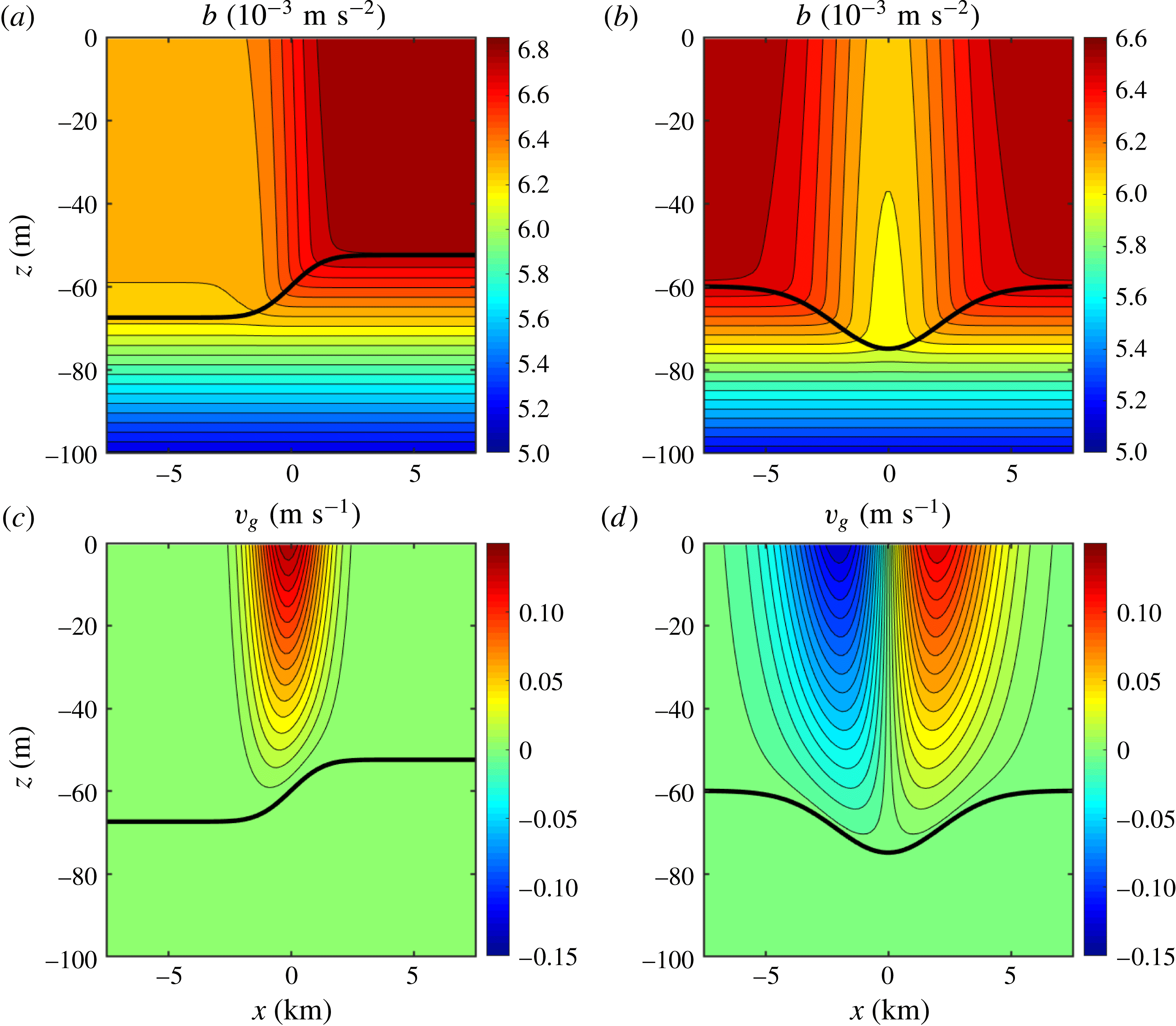
is a minimum. The corresponding along-axis geostrophic flows are a northward jet for the front and a pair of opposite-sign jets for the filament. The
 $b$
and
 $v_{g}$
fields are shown in figure 1 using the parameters in (3.7). The geostrophic Rossby number, based on the peak vertical vorticity,
 $Ro_{g}=\text{max}[\unicode[STIX]{x2202}_{x}v_{g}(x,z)]/f$
, is
 $1.3$
, and the maximum value of
 $\unicode[STIX]{x1D708}_{v}(x,z)$
is
 $0.046~\text{m}^{2}~\text{s}^{-1}$
near the centre of the boundary layer.
The convention in this paper is for the contour and colour bar ranges to correspond to the maximum absolute value of the field and be symmetric about zero, unless otherwise stated.
With
 $\unicode[STIX]{x1D708}_{v}=\unicode[STIX]{x1D705}_{v}=\boldsymbol{u}_{st}=0$
, the fields in figure 1 are steady geostrophic solutions with no secondary circulation nor frontogenetic tendency. As such they provide a dynamical template for surface fronts and filaments as coherent structures.
Idealized shapes for a 2-D front (a,c) and dense filament (b,d) with (3.5), (3.6) and (3.7):
 $b(x,z)$
(a,b) and
 $v_{g}(x,z)$
(c,d). The boundary-layer depth
 $z=-h(x)$
is indicated by the thick black line. Only a portion of the full domain is plotted. The largest surface buoyancy difference here corresponds to a surface temperature difference of 0.25
 $^{\circ }$
C for a thermal expansion coefficient of
 $\unicode[STIX]{x1D6FC}=2\times 1{0^{-4}~}^{\circ }\text{C}^{-1}$
.

For purposes of illustration a standard set of parameter values is used (n.b. the same set as in SF1):
 $$\begin{eqnarray}\displaystyle \left.\begin{array}{@{}c@{}}\displaystyle f=0.78\times 10^{-4}~\text{s}^{-1},\quad h_{0}=60~\text{m},\quad \unicode[STIX]{x1D6FF}h=15~\text{m},\quad N_{0}^{2}=3.4\times 10^{-5}~\text{s}^{-2},\\ \displaystyle N_{b}^{2}=1.0\times 10^{-7}~\text{s}^{-2},\quad b_{0}=6.4\times 10^{-3}~\text{ms}^{-2},\quad \unicode[STIX]{x1D6E4}=0.025,\quad \unicode[STIX]{x1D706}^{-1}=3~\text{m},\\ \displaystyle \unicode[STIX]{x1D708}_{v0}=1.0\times 10^{-4}~\text{m}^{2}~\text{s}^{-1},\quad u_{\ast }=0.01\,~\text{ms}^{-1},\quad \unicode[STIX]{x1D70E}_{0}=5\times 10^{-3},\quad H=250~\text{m}.\end{array}\right\} & & \displaystyle\end{eqnarray}$$
This
 $u_{\ast }$
value corresponds to an atmospheric surface wind speed of
 $U_{atm}=8.2~\text{m}~\text{s}^{-1}$
under neutral stratification conditions; its direction is
 $\unicode[STIX]{x1D703}_{\unicode[STIX]{x1D70F}}$
, with the convention that it increases anticlockwise from an origin in the east direction, and it is assumed to be uniform across the domain. To have roughly comparable values for
 $b^{\prime }(x,0)$
, maximum
 $v_{g}$
, and maximum
 $\unicode[STIX]{x1D701}_{g}=\unicode[STIX]{x2202}_{x}v_{g}$
, widths of
 $\ell =1.5$
km for the front and
 $\ell =3$
km for the dense filament are chosen. These parameter values represent a mid-sized submesoscale surface front or filament, rather than, for example, a mesoscale flow structure with a larger
 $\ell$
, smaller
 $\unicode[STIX]{x1D701}_{g}$
and
 $Ro$
values and a deeper extent reaching further below the surface boundary layer.
The surface wave field has a Stokes-drift velocity
 $\boldsymbol{u}_{st}$
. For simplicity a simple monochromatic wave is assumed (in contrast with the full wave spectrum’s profile: Webb & Fox-Kemper Reference Webb and Fox-Kemper2011), representing the peak of the wave energy spectrum at wavenumber
 $\boldsymbol{k}_{st}$
and frequency,
 $\unicode[STIX]{x1D714}_{st}=\sqrt{g|\boldsymbol{k}_{st}|}$
in deep water; the direction of
 $\boldsymbol{k}$
is defined as
 $\widehat{\unicode[STIX]{x1D703}}_{s}$
with an anticlockwise angle from east
 $\unicode[STIX]{x1D703}_{st}$
. Associated with this wave field is a Stokes-drift profile,
 $$\begin{eqnarray}\displaystyle \boldsymbol{u}_{st}=U_{st}\exp [2|\boldsymbol{k}_{st}|z]\widehat{\unicode[STIX]{x1D703}}_{st}. & & \displaystyle\end{eqnarray}$$
By weakly nonlinear wave theory,
 $U_{st}=\unicode[STIX]{x1D714}_{st}|\boldsymbol{k}_{st}|a_{st}^{2}$
, where
 $a_{st}$
is the elevation amplitude. An important condition is wind–wave equilibrium (WWE), where consistent with the previous assumption of horizontally uniform
 $\unicode[STIX]{x1D749}$
, the wave properties are also assumed to be uniform, aligned with the wind
 $\unicode[STIX]{x1D703}_{st}=\unicode[STIX]{x1D703}_{\unicode[STIX]{x1D70F}}$
, and
 $$\begin{eqnarray}\displaystyle U_{st}=u_{\ast }La_{wwe}^{-2}, & & \displaystyle\end{eqnarray}$$
where the turbulent Langmuir number
 $La_{wwe}\approx 0.32$
from measurements (Belcher et al.
Reference Belcher, Grant, Hanley, Fox-Kemper, Van Roekel, Sullivan, Large, Brown, Hines and Calvert2012). This assumption of spatial uniformity neglects the current feedback on the wind and waves, as is suitable for sufficiently long waves and weak currents (§ 6). Thus, from (3.7),
 $U_{st}=0.1~\text{m}~\text{s}^{-1}$
is a consistent Stokes velocity value in WWE. Accompanying wave parameters are
 $k_{st}=0.079~\text{m}^{-1}$
(80 m wavelength),
 $\unicode[STIX]{x1D714}_{st}=0.88~\text{s}^{-1}$
(7.2 s period) and
 $a_{st}=1.2$
m. These wave parameter choices for our solutions of interest, together with the
 $h$
value in (3.7), imply that the vertical extent of appreciable Stokes drift is much less than the ‘mixed-layer’ depth, which is the usual oceanic situation.
In real WWE the surface wave spectrum is broadband, and the associated Stokes-drift profile
 $\boldsymbol{u}_{st}(z)$
has a somewhat different shape to (3.8). Accordingly the SCFT solutions with WEC would have somewhat different shapes to those in § 5, but experience with large-eddy simulations of Langmuir turbulence indicate that the general patterns and amplitudes would not be very different.
In the following sections, the TTW +
 $\unicode[STIX]{x1D6FA}$
E diagnostic system is solved for both
 $\boldsymbol{u}_{3}$
and
 ${\mathcal{T}}$
with the
 $b(x,z)$
field specified in (3.5)–(3.7) for various wind stress, eddy diffusion and Stokes-drift combinations. As in SF1 the numerical discretization of this system is based on centred finite differences of second-order accuracy in the grid size. For the solutions shown in this paper, the horizontal grid resolution is
 $\text{d}x=160$
m and the finest vertical grid interval near the surface is
 $\text{d}z=0.5$
m. These are fine enough to resolve the SCFT solution features, with only small changes of a few per cent in the quantitative results with further grid refinement.
4 Turbulent thermal wind (TTW)
In its simplest expression the TTW balance is hydrostatic in vertical momentum; a combination of pressure gradient, Coriolis force and vertical momentum mixing in horizontal momentum; and incompressible mass balance. In the 2-D TTW +
 $\unicode[STIX]{x1D6FA}$
E system, these balances are augmented by surface wind stress,
 $wN^{2}$
buoyancy advection and vertical buoyancy mixing, if not also nonlinear ageostrophic momentum and buoyancy advection.
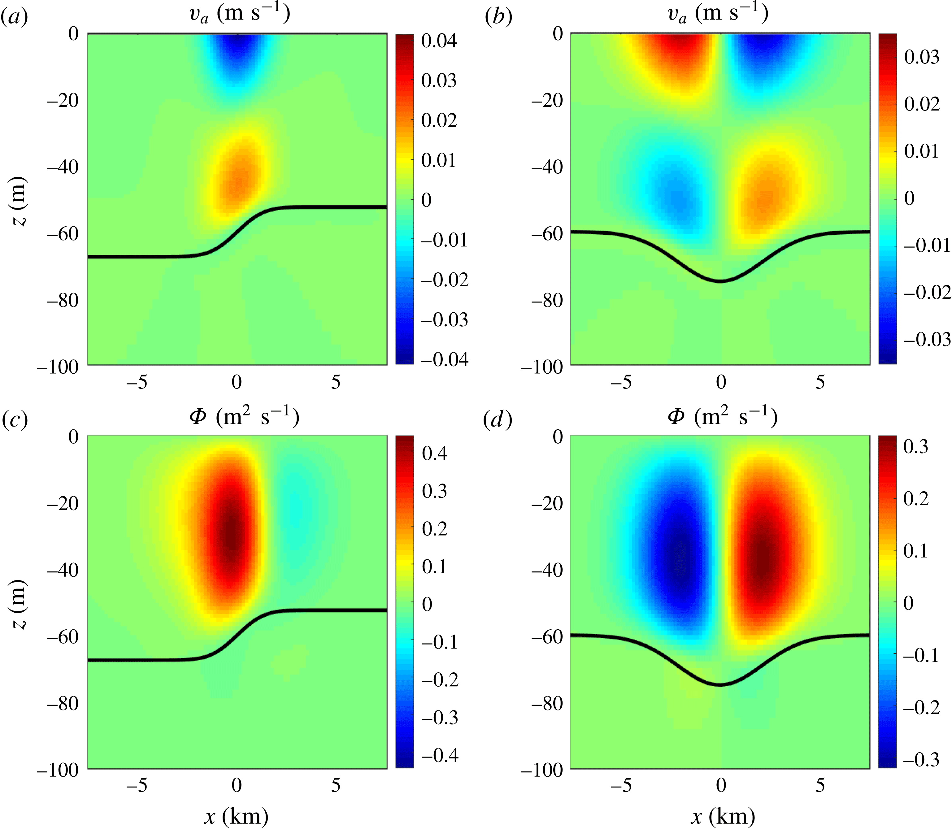
Linear TTW secondary ageostrophic circulation for (a,c) a front and (b,d) a dense filament, corresponding to the respective
 $b^{\prime }(x,z)$
fields in figure 1: (a,b)
 $v_{a}(x,z)$
and (c,d)
 $\unicode[STIX]{x1D6F7}(x,z)$
. Again and throughout the paper,
 $z=-h(x)$
is indicated by the thick black line. In these solutions the surface stress
 $\unicode[STIX]{x1D749}=0$
, but the vertical mixing fields
 $(\unicode[STIX]{x1D708}_{v},\unicode[STIX]{x1D705}_{v})$
are as specified in (3.4)–(3.7). WEC is neglected with
 $\boldsymbol{u}_{st}=0$
here, and nonlinear advection is neglected in the right-hand sides of (2.10) and (2.13). Also,
 $\unicode[STIX]{x1D749}=0$
here.

This dynamics is the subject of SF1, and it is briefly recalled here to set the context for additional WEC influences. The essential result is that vertical momentum mixing in the presence of a submesoscale
 $b(x,z)$
induces a secondary circulation that effects both vertical and horizontal buoyancy fluxes across the front or filament, and further induces velocity and buoyancy frontogenesis. The ageostrophic circulations associated with the
 $b$
and
 $v_{g}$
fields in figure 1 are shown in figure 2 for the simplest case with
 $\unicode[STIX]{x1D749}=0$
and neglected advection.
The secondary circulation is localized near the submesoscale
 $b^{\prime }$
anomaly with no far-field flow,
 $\boldsymbol{u}_{\infty }=0$
. The along-axis
 $v_{a}$
diminishes the geostrophic vertical shear across the boundary layer, and it diminishes the peak Rossby number,
 $Ro=\text{max}[\unicode[STIX]{x2202}_{x}v(x,z)]/f$
, by approximately one third. The cross-plane circulation is 2-D incompressible, so is represented with an overturning streamfunction
 $\unicode[STIX]{x1D6F7}(x,z)$
defined by
 $$\begin{eqnarray}\displaystyle u_{a}=\unicode[STIX]{x2202}_{z}\unicode[STIX]{x1D6F7}\quad \text{and}\quad w=-\unicode[STIX]{x2202}_{x}\unicode[STIX]{x1D6F7}. & & \displaystyle\end{eqnarray}$$
A front has a single overturning cell with downwelling on the dense side, while a dense filament has two cells with especially strong downwelling in the centre.
Because the SCFT behaviours of fronts and filaments are so functionally similar (e.g. a filament is approximately a double front), examining only one of these configurations is often good enough to be able to imagine the other, while keeping in mind that profile shape differences do have moderate quantitative consequences.
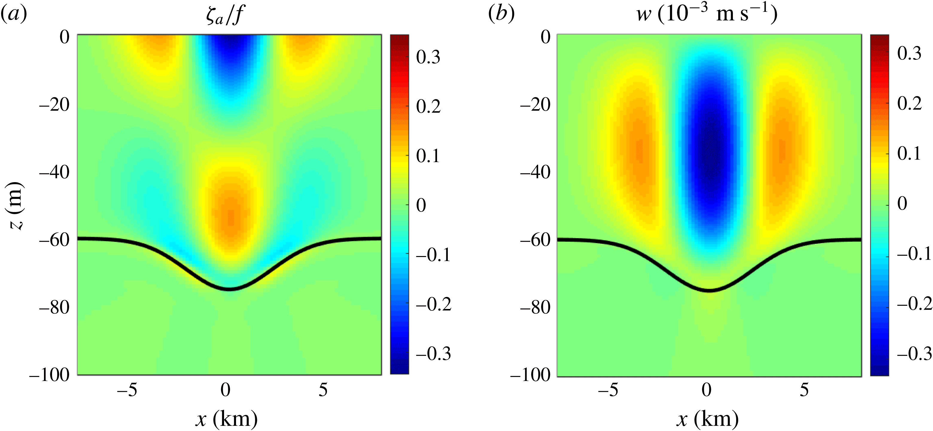
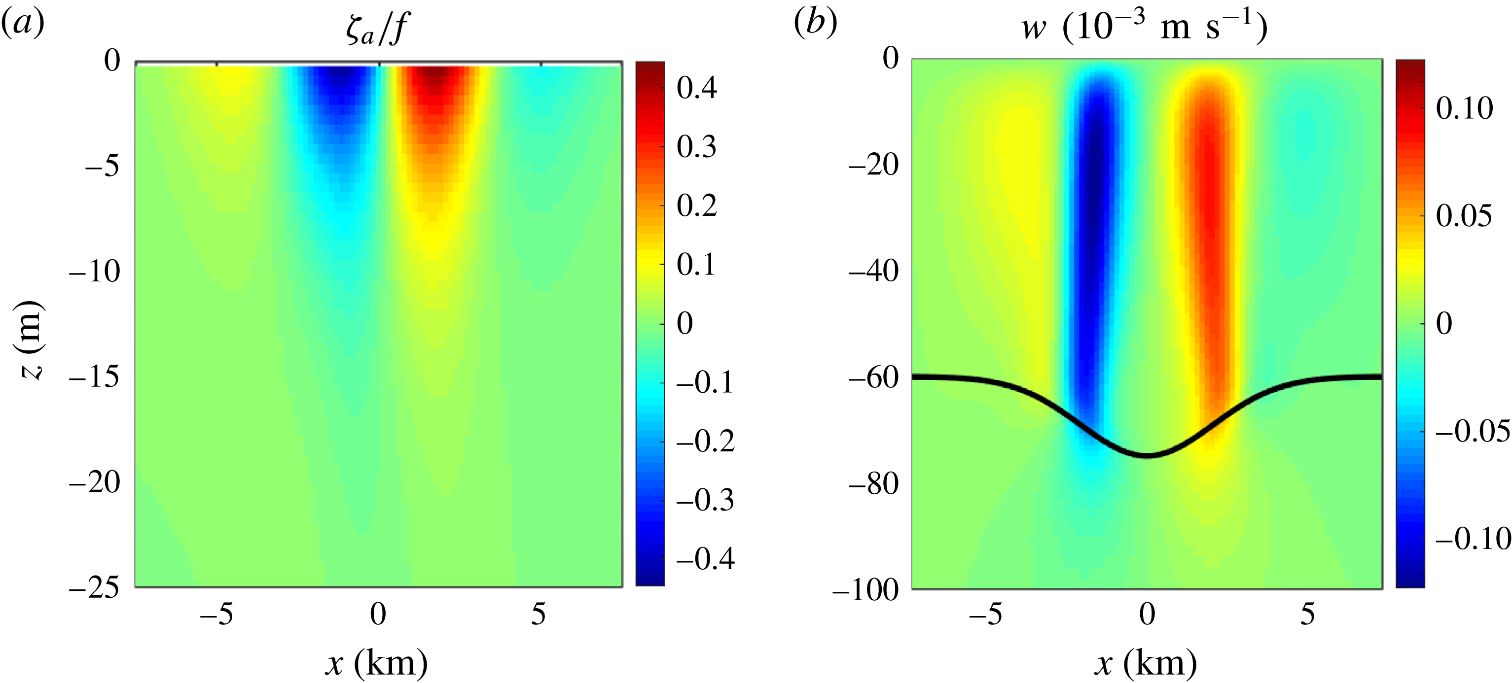
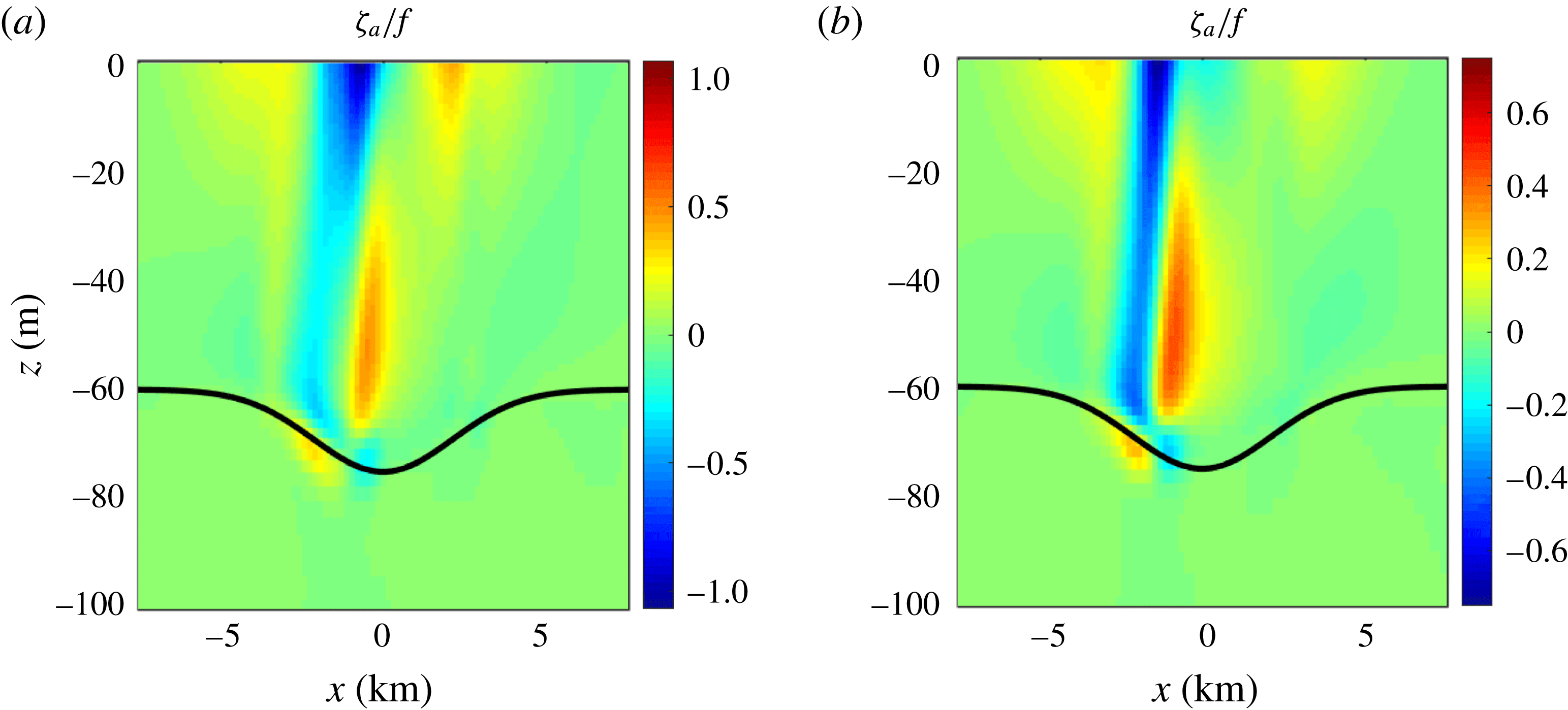
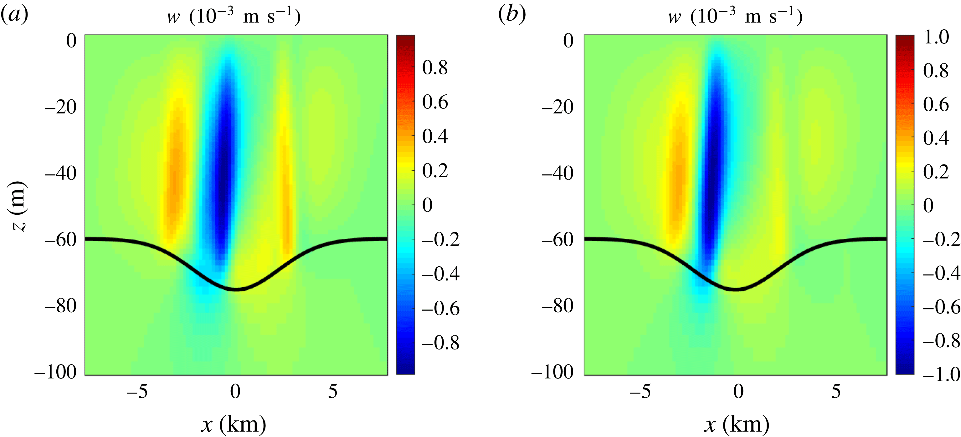
Ageostrophic vorticity normalized by
 $f$
(a), and vertical velocity (b) for a dense filament in the same linear TTW solution with the other fields shown in the right columns of figures 1 and 2.
 $z=-h(x)$
is indicated by the thick black line.
 $\unicode[STIX]{x1D749}=\boldsymbol{u}_{st}=0$
here.

For the subsequent assessments of WEC effects and their parameter dependencies in § 5, it is useful to also look at the derivative fields for the ageostrophic circulation elements in figure 2, i.e. the ageostrophic vorticity,
 $\unicode[STIX]{x1D701}_{a}=\unicode[STIX]{x2202}_{x}v_{a}$
, and the vertical velocity,
 $w=-\unicode[STIX]{x2202}_{x}\unicode[STIX]{x1D6F7}$
. In figure 3, these fields are shown for a dense filament. The incremental effect of
 $\unicode[STIX]{x1D701}_{a}$
is to diminish the vertical gradient in the geostrophic vorticity
 $\unicode[STIX]{x1D701}_{g}=\unicode[STIX]{x2202}_{x}v_{g}$
, which itself has a surface-intensified tripole pattern with cyclonic vorticity in the centre.
 $w$
has a strong central downwelling with weaker peripheral upwelling on both sides;
 $w$
has its largest speed in the middle of the surface boundary layer.
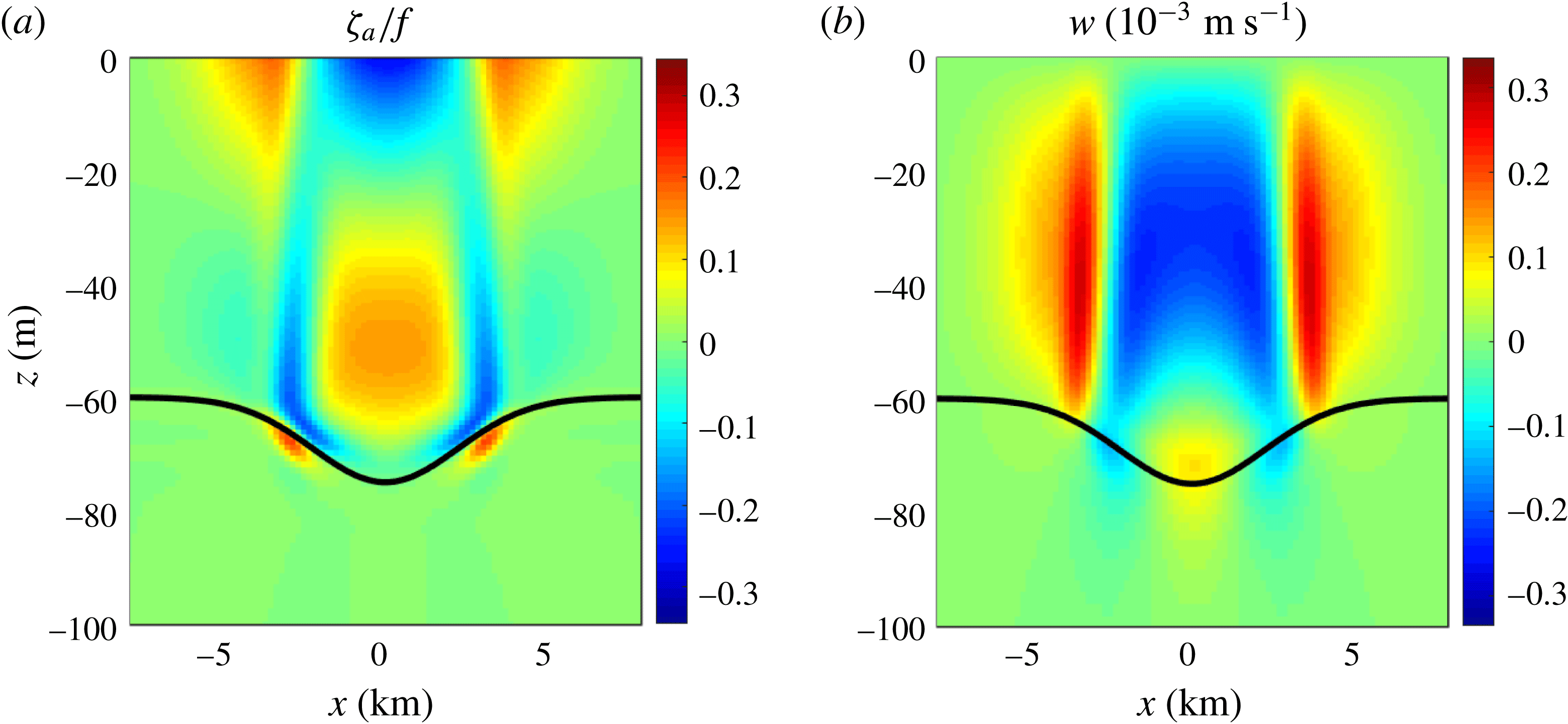
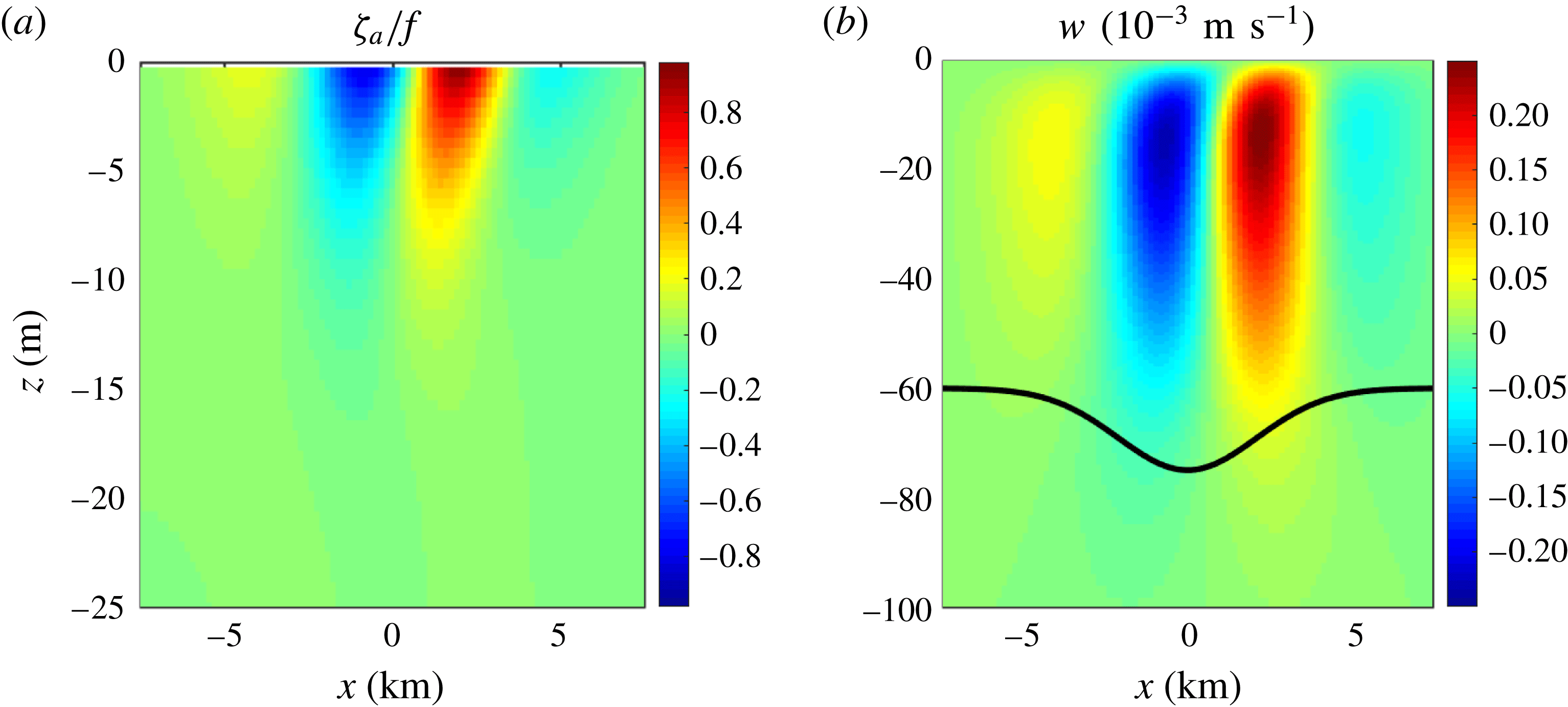
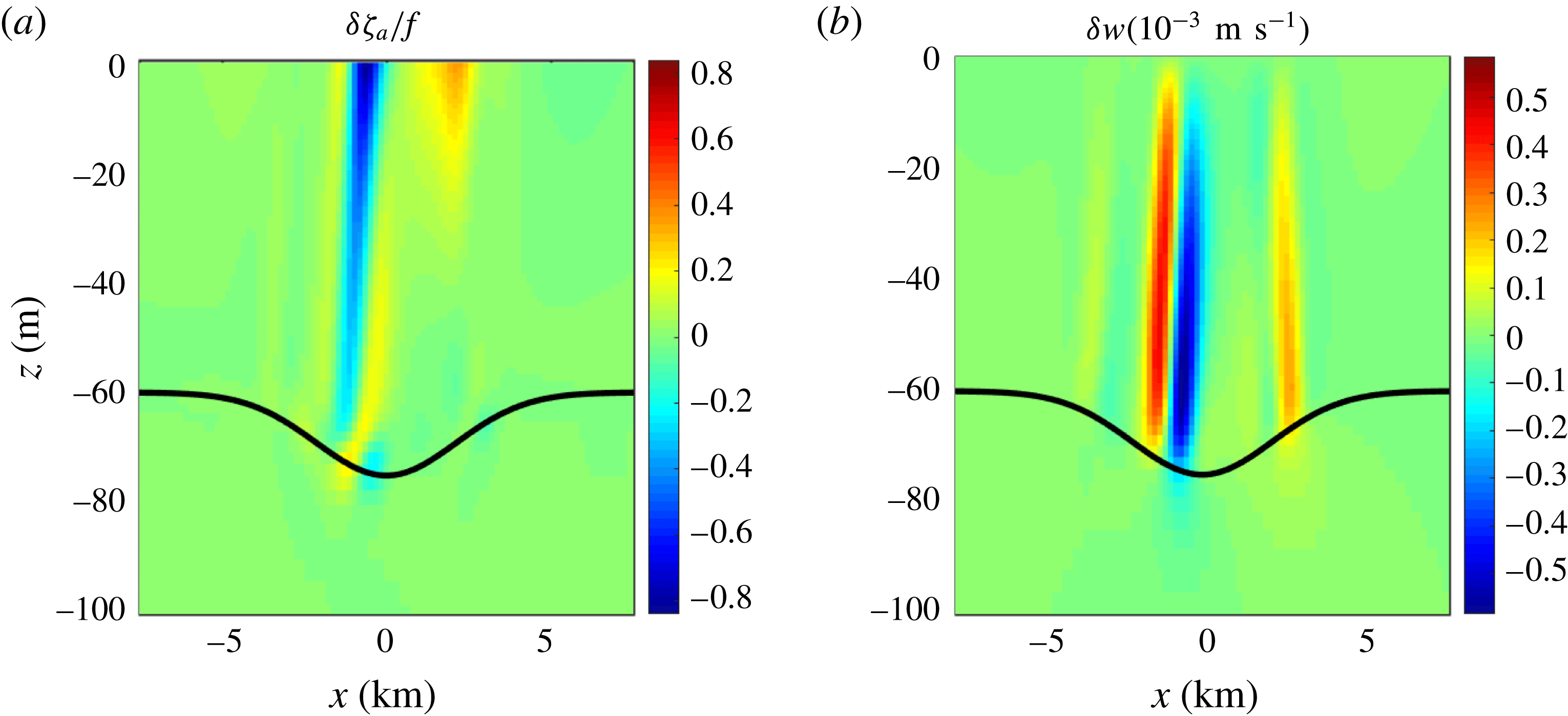
Ageostrophic vorticity normalized by
 $f$
(a), and vertical velocity (b) for a dense filament in a fully nonlinear TTW solution, to be compared with the linear solution in figure 3.
 $z=-h(x)$
is indicated by the thick black line.
 $\unicode[STIX]{x1D749}=\boldsymbol{u}_{st}=0$
here. The colour bar ranges here are chosen to match those in figure 3.

Because
 $Ro\approx 1$
in this TTW solution with the parameters in (3.7), the neglect of nonlinear ageostrophic advection of momentum and buoyancy is not defensible, except as a means of clarifying the important influences. In a fully nonlinear SCFT solution (figure 4), the advective effects primarily act to modify the shapes of the pattern extrema without appreciably changing the general morphology or magnitude compared to the linear solution. (With wind stress or WEC also included, the advective changes are more substantial: see SF1, § 6 and §§ 5.2–5.4 below. With TTW only (i.e. front/filament plus mixing), the nonlinear modification to the linear solution is weaker than it can be with either WEC or wind-stress added when the wave or wind orientation is favourable to an enhanced secondary circulation.) As
 $Ro$
decreases, the secondary circulation decreases linearly in amplitude, and the advective shape modifications also diminish.
5 Wave effects on the currents
In McWilliams & Fox-Kemper (Reference McWilliams and Fox-Kemper2013) the WEC problems of the adjustment of steady 2-D geostrophic, hydrostatic surface fronts and filaments to the imposition of
 $\boldsymbol{u}_{st}(z)$
are solved under assumptions of conservative dynamics, steady homogeneous waves and a steady final state. The solution has the form of
 $$\begin{eqnarray}\displaystyle \left.\begin{array}{@{}c@{}}\displaystyle b(x,z)=b_{0}(x,z)+b_{1}(x,z),\quad u(x,z)=-u_{st}(z),\\ \displaystyle v(x,z)=v_{0}(x,z)-v_{st}(z)+v_{1}(x,z),\quad w(x,z)=0.\end{array}\right\} & & \displaystyle\end{eqnarray}$$
It is comprised of an initial geostrophic balance between
 $b_{0}$
and
 $v_{0}$
, an anti-Stokes flow,
 $-\boldsymbol{u}_{st}$
, due to the Stokes–Coriolis force, and a rearranged ageostrophic balance between
 $b_{1}$
and
 $v_{1}$
that includes the Stokes vortex force and Stokes buoyancy advection. When a frontal flow structure is present, the modifications
 $b_{1}$
and
 $v_{1}$
arise through an adjustment process instigated by the imposition of surface waves on
 $b_{0}$
and
 $v_{0}$
that conserves the buoyancy and potential vorticity of each fluid parcel. For weak
 $U_{st}$
,
 $b_{1}$
and
 $v_{1}$
have an asymptotic normalized amplitude of order
 $$\begin{eqnarray}\displaystyle \unicode[STIX]{x1D700}=\frac{U_{st}h}{f\ell h_{st}} & & \displaystyle\end{eqnarray}$$
relative to the initial geostrophic components, where
 $h$
is the vertical scale of the frontal flow and
 $h_{st}=1/(2k_{st})$
is the vertical scale of the Stokes drift. In an analysis with
 $1\gtrsim \unicode[STIX]{x1D700}\gg Ro$
, the adjustment fields
 $b_{1}$
and
 $v_{1}$
have opposite
 $x$
-symmetries to those of
 $b_{0}$
and
 $v_{0}$
; e.g. for a geostrophic front with even symmetric
 $v_{0}(x,z)$
,
 $v_{1}$
is odd symmetric, and vice versa for
 $b_{0}$
and
 $b_{1}$
. For a filament all four of these components have the opposite
 $x$
-symmetries as for a front. The adjustment fields are largest when the frontal vertical scale is close to the stratification mixed-layer depth (referred to as a ‘sweet spot’), as assumed here and as typical of surface submesoscale currents. Their
 $(x,z)$
spatial extent corresponds approximately to that of the initial geostrophic flow.
The WEC SCFT problems posed here are different in that
 $b(x,z)$
and
 $\boldsymbol{u}_{st}(z)$
are specified (along with the surface fluxes and vertical mixing coefficients), and the balanced circulation
 $(\boldsymbol{u},w)$
is diagnosed. This diagnosed circulation is dynamically both non-conservative and non-steady except in the no-mixing limit. It has a conservative solution with
 $b_{1}=0$
and a
 $v_{1}\neq 0$
as determined in § 5.2.
The role of an anti-Stokes flow in a Stokes–Ekman layer, in particular its contribution of a vertically integrated horizontal transport that cancels the Stokes-drift transport, is demonstrated in Huang (Reference Huang1979) and elaborated on in McWilliams, Sullivan & Moeng (Reference McWilliams, Sullivan and Moeng1997), Polton, Lewis & Belcher (Reference Polton, Lewis and Belcher2005) and Wenegrat & McPhadden (Reference Wenegrat and McPhadden2016). Without wind stress, mixing and a frontal buoyancy gradient
 $b_{0}$
, the anti-Stokes flow in (5.1) exactly balances
 $\boldsymbol{u}_{st}(z)$
at every depth, but when any of these other influences are present, it usually has a different vertical profile (§§ 5.1–5.4).
5.1 Far-field Stokes–Ekman boundary layer
In the
 $x$
far field,
 $\unicode[STIX]{x2202}_{x}b=v_{g}=0$
, and
 $\unicode[STIX]{x1D749}$
, (
 $\unicode[STIX]{x1D708}_{v},\unicode[STIX]{x1D705}_{v}$
) and
 $\boldsymbol{u}_{st}$
are horizontally uniform; hence
 $w={\mathcal{T}}=0$
(i.e. no SCFT). In this case the 2-D horizontal momentum balance simplifies to
 $$\begin{eqnarray}\displaystyle \left.\begin{array}{@{}c@{}}\displaystyle f\hat{\boldsymbol{z}}_{3}\times (\boldsymbol{u}+\boldsymbol{u}_{st})=\unicode[STIX]{x2202}_{z}[\unicode[STIX]{x1D708}_{v}\unicode[STIX]{x2202}_{z}\boldsymbol{u}],\\ \displaystyle \unicode[STIX]{x1D708}_{v}\unicode[STIX]{x2202}_{z}\boldsymbol{u}=\frac{1}{\unicode[STIX]{x1D70C}_{0}}\,\unicode[STIX]{x1D749}\quad \text{at}~z=0,\\ \displaystyle \unicode[STIX]{x2202}_{z}\boldsymbol{u}=0\quad \text{at}~z=-H,\end{array}\right\} & & \displaystyle\end{eqnarray}$$
which is called the Stokes–Ekman-layer model whose ageostrophic solution
 $\boldsymbol{u}_{a}=\boldsymbol{u}$
is designated as
 $\boldsymbol{u}_{\infty }(z)$
. The vertical integral yields the horizontal transport,
 $$\begin{eqnarray}\displaystyle \mathbf{T}_{\infty }=\int _{-H}^{0}\boldsymbol{u}_{\infty }(z)\,\text{d}z=\hat{\boldsymbol{z}}_{3}\times \frac{\unicode[STIX]{x1D749}}{f\unicode[STIX]{x1D70C}_{0}}-\int _{-H}^{0}\boldsymbol{u}_{st}\,\text{d}z. & & \displaystyle\end{eqnarray}$$
The right-hand side terms are the Ekman transport perpendicular to the surface stress and the anti-Stokes transport. Thus, a degree of anti-Stokes flow in
 $\boldsymbol{u}$
is expected, but it need not occur pointwise in
 $z$
because of the mixing in (5.3).
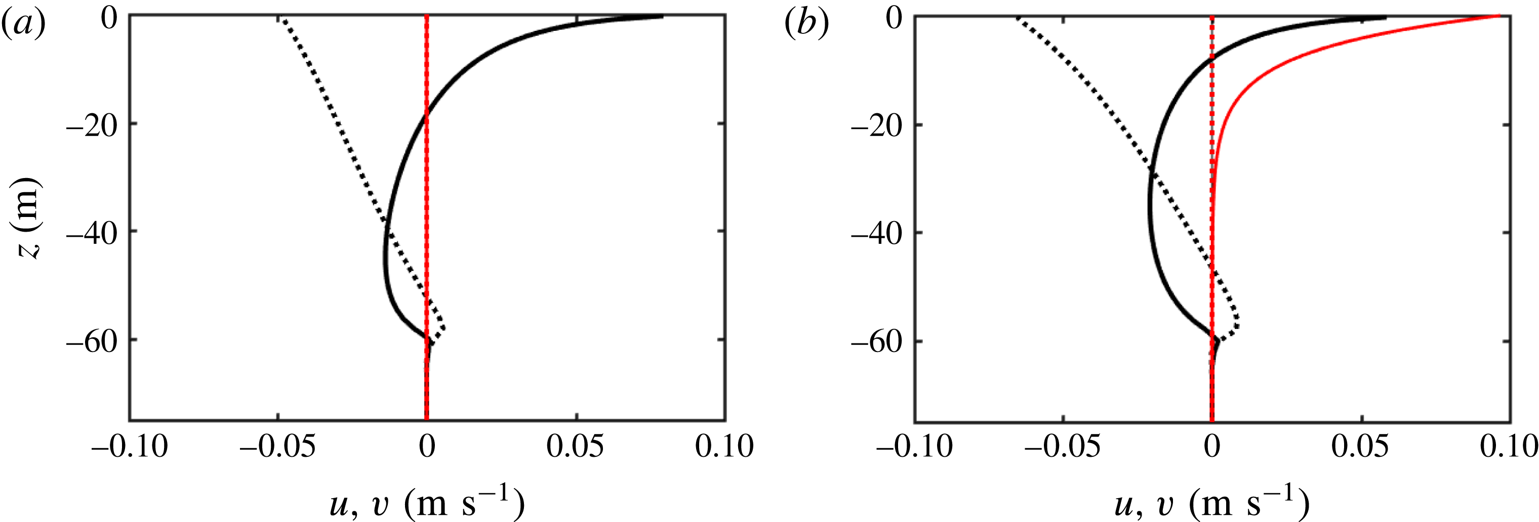
Vertical profiles of the velocity
 $\boldsymbol{u}_{\infty }(z)$
in the homogeneous
 $x$
far field for (a) an Ekman layer and (b) a Stokes–Ekman layer in WWE.
 $u_{\infty }$
is solid black, and
 $v_{\infty }$
is dotted black. The boundary-layer depth is
 $h_{0}=60$
m,
 $u_{\ast }=0.01~\text{m}~\text{s}^{-1}$
,
 $\unicode[STIX]{x1D703}_{\unicode[STIX]{x1D70F}}=0$
and the maximum value of
 $\unicode[STIX]{x1D708}_{v}(z)$
is
 $0.036~\text{m}^{2}~\text{s}^{-1}$
in the far field – all consistent with (3.7). The
 $u_{st}(z)$
and
 $v_{st}(z)$
profiles with
 $\unicode[STIX]{x1D703}_{st}=0$
are the solid and dotted red curves.

In WWE
 $\unicode[STIX]{x1D749}$
and
 $\boldsymbol{u}_{st}$
are aligned, and
 $\boldsymbol{u}_{\infty }$
simply rotates with
 $\unicode[STIX]{x1D703}_{\unicode[STIX]{x1D70F}}$
. Figure 5 shows a comparison of an Ekman-layer solution (for
 $\unicode[STIX]{x1D703}_{\unicode[STIX]{x1D70F}}=0$
) to a WWE Stokes–Ekman solution. They are approximately similar in shape, although the down-wind/wave velocity deepens and shifts more negatively with
 $\boldsymbol{u}_{st}\neq 0$
, the latter as expected from the anti-Stokes transport in (5.4). Thus, both wind and wave influences are consequential in WWE, with perhaps a somewhat greater influence by the wind.
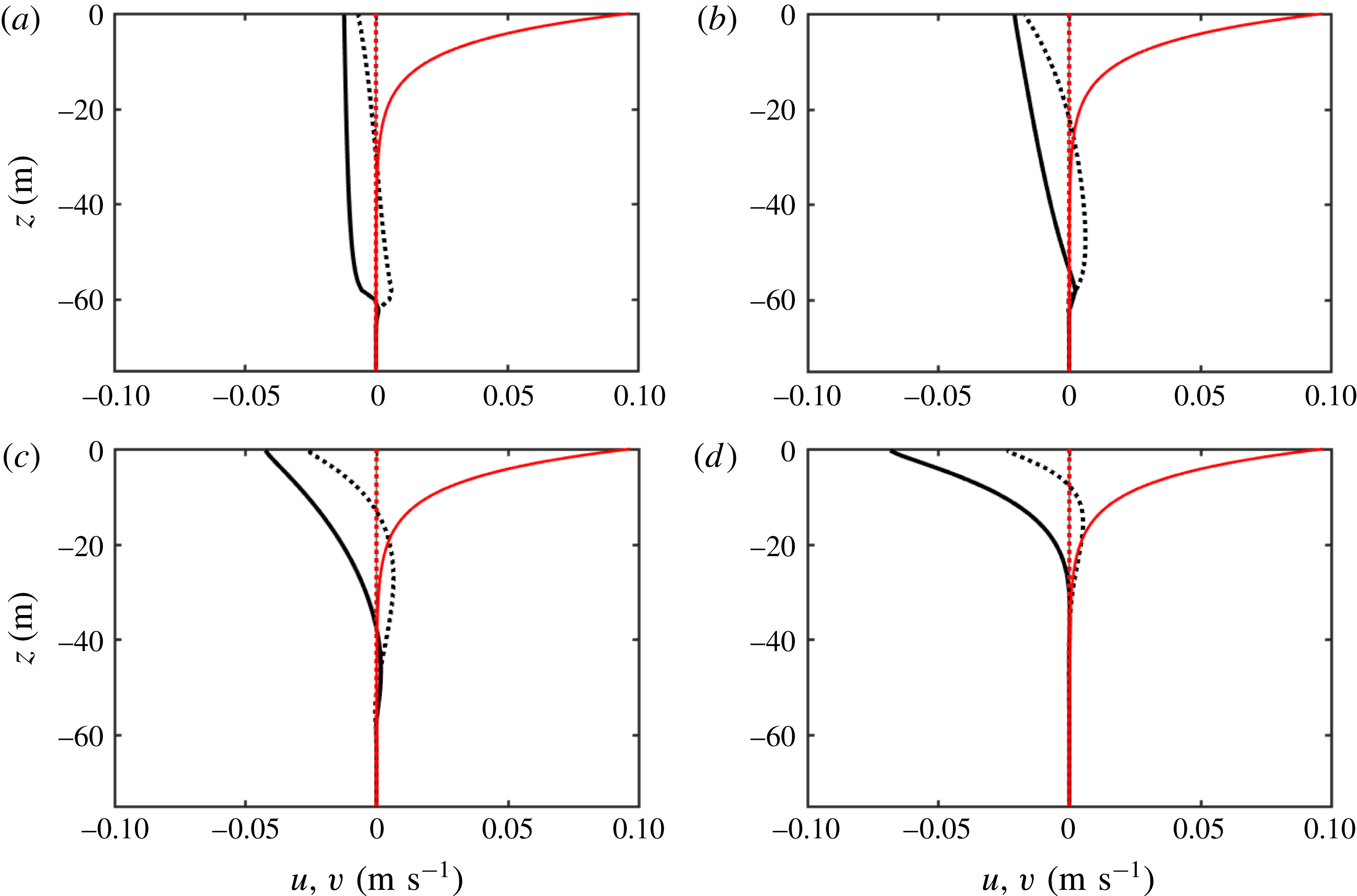
Vertical profiles of the Stokes-layer velocity
 $\boldsymbol{u}_{\infty }(z)$
in the homogeneous
 $x$
far field for
 $\unicode[STIX]{x1D749}=0$
in the surface stress condition, but with
 $\unicode[STIX]{x1D708}_{v}(z)$
profiles corresponding to multiples of the standard
 $u_{\ast }$
value in (3.4) and (3.7): 4
 $\times$
(a), 1
 $\times$
(b), 0.25
 $\times$
(c) and 0.0625
 $\times$
(d).
 $u_{\infty }$
is solid black, and
 $v_{\infty }$
is dotted black. The red
 $\boldsymbol{u}_{st}(z)$
profile is the same as in figure 5(b). As
 $\unicode[STIX]{x1D708}_{v}\rightarrow 0$
,
 $\boldsymbol{u}_{\infty }(z)\rightarrow -\boldsymbol{u}_{st}(z)$
.

In a realistic WWE state there is a broad wavenumber spectrum for the surface wave field, and this alters the
 $\boldsymbol{u}_{st}(z)$
profile by enhancing its near-surface shear compared to the simple spectrum-peak profile in (3.8) (Kenyon Reference Kenyon1969). However, the resulting
 $\boldsymbol{u}_{\infty }(z)$
profile is not very sensitive to the shape of
 $\boldsymbol{u}_{st}(z)$
because of the vertical spreading effect of diffusion in (5.3).
In the ocean
 $\unicode[STIX]{x1D749}$
and
 $\unicode[STIX]{x1D708}_{v}$
can vary independently, partly because of a disequilibrium adjustment of the turbulent layer to wind changes, but more persistently because of a convective forcing (i.e.
 ${\mathcal{B}}<0$
) that enhances
 $\unicode[STIX]{x1D708}_{v}$
over its equilibrium wind magnitude (e.g. as in the (3.4) specification).
Even in the limit of weak wind stress (or large swell),
 $\boldsymbol{u}_{\infty }$
persists. This case can be referred to as the Stokes boundary layer. This is shown in figure 6, where
 $\unicode[STIX]{x1D749}$
is set to zero, and the
 $\unicode[STIX]{x1D708}_{v}(z)$
profile from (3.4) and (3.7) is rescaled by a multiplicative constant. The surface velocity
 $\boldsymbol{u}_{\infty }(0)$
is rotated anticlockwise (if
 $f>0$
) from the opposite direction to
 $\boldsymbol{u}_{st}(0)$
, and with increasing depth there is a modest rotation of
 $\boldsymbol{u}_{\infty }(z)$
clockwise. The down-wave component
 $u_{\infty }(z)$
is persistently in the opposite direction to
 $\boldsymbol{u}_{st}$
, but its shape is less surface-intensified. For stronger eddy diffusion, the
 $\boldsymbol{u}_{\infty }(z)$
profile extends deeper into the surface layer, while as
 $\unicode[STIX]{x1D708}_{v}\rightarrow 0$
the profile approaches an anti-Stokes profile pointwise, although the progression is slow in the diffusivity magnitude. This result is largely anticipated in Polton et al. (Reference Polton, Lewis and Belcher2005).
As a basis for explaining the qualitative
 $\boldsymbol{u}_{\infty }(z)$
shapes, analytic solutions for constant
 $\unicode[STIX]{x1D708}_{v}$
are recorded in appendix A. They demonstrate that
 $\boldsymbol{u}_{\infty }\rightarrow -\boldsymbol{u}_{st}$
as
 $\unicode[STIX]{x1D708}_{v}\rightarrow 0$
and
 $\boldsymbol{u}_{\infty }\rightarrow -U_{st}/(2k_{st}h)$
as
 $\unicode[STIX]{x1D708}_{v}\rightarrow \infty$
in the Stokes layer, consistent with the profile shapes in figure 6(a,d). They also provide a scaling estimate for the relative magnitude
 ${\mathcal{R}}$
of Stokes- and Ekman-layer velocities. When the wind is weak, the turbulent Ekman-layer depth
 $h_{ek}$
shrinks as
 $u_{\ast }/f<h$
, the velocity
 $\boldsymbol{u}\sim u_{\ast }$
and
 ${\mathcal{R}}\sim La^{-2}$
. When the wind and/or turbulence is strong, the turbulent-layer thickness is limited by
 $h$
through the underlying stratification, and
 ${\mathcal{R}}\sim La^{-2}(f/u_{\ast }k_{st})$
, with the last factor usually small; this ratio is independent of
 $\unicode[STIX]{x1D708}_{v}$
in this limit.
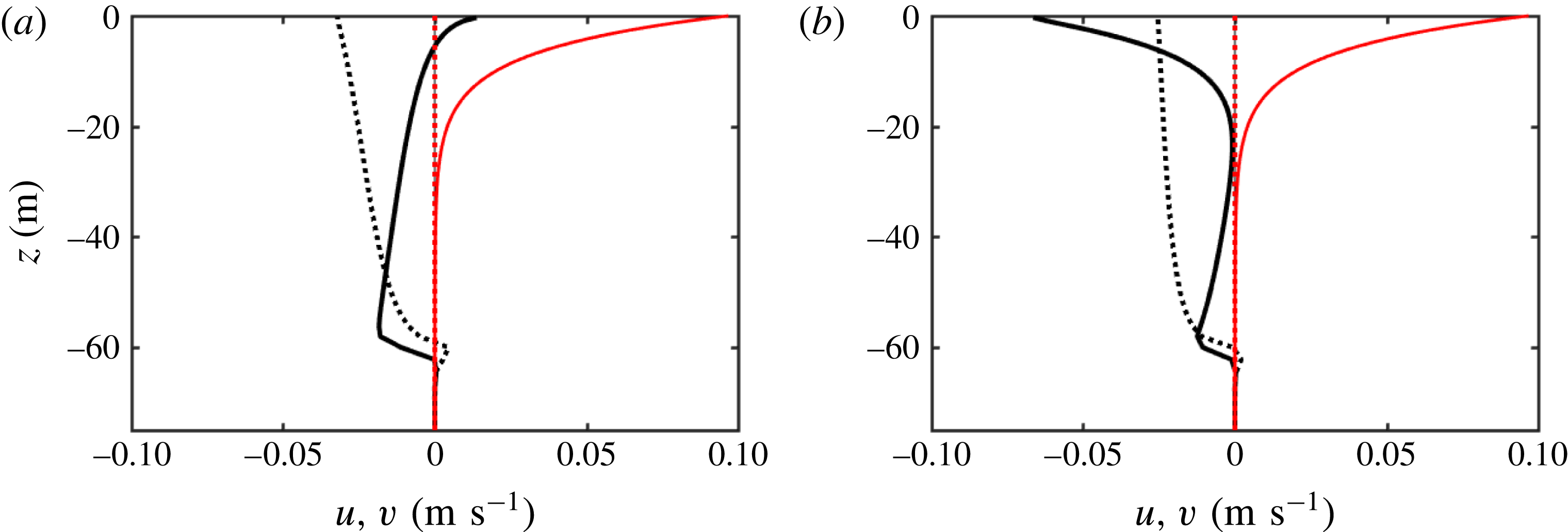
Vertical profiles of the velocity
 $\boldsymbol{u}_{\infty }(z)$
in the homogeneous
 $x$
far field for a Stokes–Ekman layer in WWE with two different modifications of the parameterization of
 $\unicode[STIX]{x1D708}_{v}(z)$
: (a) a multiplicative magnitude enhancement by 4
 $\times$
(case (i) defined in the text) and (b) in addition a replacement of the mixing force by
 $\unicode[STIX]{x2202}_{z}[\unicode[STIX]{x1D708}_{v}\unicode[STIX]{x2202}_{z}(\boldsymbol{u}+\boldsymbol{u}_{st})]$
(case (i)
 $+$
(ii)).
 $u_{\infty }$
is solid black, and
 $v_{\infty }$
is dotted black. The boundary-layer depth is
 $h_{0}=60$
m,
 $u_{\ast }=0.01~\text{m}~\text{s}^{-1}$
,
 $\unicode[STIX]{x1D703}_{\unicode[STIX]{x1D70F}}=0$
and the maximum value of
 $\unicode[STIX]{x1D708}_{v}(z)$
is
 $0.144~\text{m}^{2}~\text{s}^{-1}$
. The
 $u_{st}(z)$
and
 $v_{st}(z)$
profiles with
 $\unicode[STIX]{x1D703}_{st}=0$
are the solid and dotted red curves.

After many published large eddy simulation (LES) studies of Langmuir turbulence (LT), it is clear that the prevailing eddy viscosity parameterizations should be modified in the presence of surface waves; i.e. in the terminology of Reichl et al. (Reference Reichl, Wang, Hara, Ginis and Kukulka2016), KPP needs to be generalized to a KPP-LT. As yet there is no consensus about what a realistic KPP-LT should entail, though preliminary proposals abound (McWilliams & Sullivan Reference McWilliams and Sullivan2000; Smyth et al.
Reference Smyth, Skyllingstad, Crawford and Wijesekera2002; Roekel et al.
Reference Van Roekel, Fox-Kemper, Sullivan, Hamlington and Haney2012; McWilliams et al.
Reference McWilliams, Huckle, Liang and Sullivan2012; McWilliams et al.
Reference McWilliams, Huckle, Liang and Sullivan2014; Reichl et al.
Reference Reichl, Wang, Hara, Ginis and Kukulka2016; Li & Fox-Kemper Reference Li and Fox-Kemper2017), and some other LT proposals are made outside the KPP framework (Harcourt Reference Harcourt2013, Reference Harcourt2015). In advance of a more mature form of KPP-LT, it is informative to do some preliminary scouting of some aspects of its likely consequences. So, now consider two variants of the Stokes–Ekman model that modify
 $\unicode[STIX]{x1D708}_{v}$
in ways that seem qualitatively well supported by the existing LES studies and parameterization proposals.
(i) The magnitude of
 $\unicode[STIX]{x1D708}_{v}$
increases in WWE compared to Ekman layers without WEC.
(ii) The profile of
$-\overline{\boldsymbol{u}^{\prime }w^{\prime }}(z)$
in WWE is more simply represented by an eddy-diffusive flux of the Lagrangian mean current rather than the Eulerian one; i.e. the horizontal momentum mixing terms in (2.4) and (5.3) should be replaced by
$\unicode[STIX]{x2202}_{z}[\unicode[STIX]{x1D708}_{v}\unicode[STIX]{x2202}_{z}(\boldsymbol{u}+\boldsymbol{u}_{st})]$
, with an analogous modification of the surface boundary condition.


The second item implies an isomorphism between the Stokes–Ekman-layer problem for the Lagrangian mean velocity,
 $\boldsymbol{u}_{\infty }+\boldsymbol{u}_{st}$
, and the usual Ekman-layer problem for
 $\boldsymbol{u}_{\infty }$
.
The sensitivity of
 $\boldsymbol{u}_{\infty }(z)$
to these proposals is demonstrated in figure 7. With (i) (figure 7
a), there is a general deepening of the profile, e.g. as compared with the original-
 $\unicode[STIX]{x1D708}_{v}$
solution in figure 5(b); this is consistent with the similar deepening effect on the Stokes boundary layer in figure 6(a), and appendix A. With the combination of (i)
 $+$
(ii) (figure 7
b), the upper part of
 $\boldsymbol{u}_{\infty }(z)$
further manifests a substantial anti-Stokes shape, even in this situation with large
 $\unicode[STIX]{x1D708}_{v}$
(cf. figure 6
d).
Therefore, by comparing the range of Stokes–Ekman
 $\boldsymbol{u}_{\infty }(z)$
profiles in figures 5–7, it is clear that WEC effects can make significant changes to the familiar Ekman profile, through modifications from both the Stokes–Coriolis force and from an appropriate KPP-LT parameterization scheme as it may come to be.
5.2 Conservative Stokes secondary circulation
As explained in McWilliams & Fox-Kemper (Reference McWilliams and Fox-Kemper2013), a conservative, steady-state, nonlinear WEC solution of (2.4) exists when
 $\unicode[STIX]{x1D708}_{v}=\unicode[STIX]{x1D705}_{v}=\unicode[STIX]{x1D749}=0$
and the surface wave field is steady and homogeneous. It is an exact nonlinear solution of the form (5.1), and it is a generalization of thermal-wind balance that occurs when the waves vanish, which also is an exact steady solution. However, this solution form is non-unique in general in the sense that the fields are under-determined by (2.4) given
 $\boldsymbol{u}_{st}$
. In McWilliams & Fox-Kemper (Reference McWilliams and Fox-Kemper2013) the non-uniqueness is resolved by posing the problem as an adjustment of a given thermal-wind structure to the arrival of the waves, and the approximate solutions presented there are only valid through
 $O(\unicode[STIX]{x1D700}^{2})$
with undetermined corrections at
 $O(Ro)$
. Here the non-uniqueness is resolved by the SCFT diagnostic perspective of both
 $b=b_{0}$
and
 $\boldsymbol{u}_{st}$
being specified a priori (hence
 $b_{1}=0$
), and its solution is uniformly valid in
 $\unicode[STIX]{x1D700}$
and
 $Ro$
.
The SCFT ageostrophic correction field
 $v_{1}$
in a solution of the form (5.1) is determined by the linear partial differential equation (PDE),
 $$\begin{eqnarray}\displaystyle f\unicode[STIX]{x2202}_{z}v_{1}+(\unicode[STIX]{x2202}_{z}v_{st})\unicode[STIX]{x2202}_{x}v_{1}=-\unicode[STIX]{x1D701}_{g}\unicode[STIX]{x2202}_{z}v_{st}. & & \displaystyle\end{eqnarray}$$
After subtracting the geostrophic, hydrostatic and Stokes–Coriolis balances, this is a WEC-generalized form of thermal-wind balance that is valid for a 2-D steady nonlinear conservative combination of the
 $x$
- and
 $z$
-momentum equations in (2.4). The occurrence of a non-trivial
 $v_{1}$
is caused by the Stokes vortex force in (2.1) in the presence of a geostrophic frontal flow with
 $\unicode[STIX]{x1D701}_{g}\neq 0$
. A scaling estimate for the relative magnitude of
 $v_{1}$
compared to
 $v_{g}$
comes from balancing the first left-side term with the right-hand side forcing, viz.,
 $$\begin{eqnarray}\displaystyle \widehat{\unicode[STIX]{x1D700}}=\frac{U_{st}}{f\ell }\sim \frac{V_{1}}{V_{g}}, & & \displaystyle\end{eqnarray}$$
which is generally smaller than the adjustment magnitude
 $\unicode[STIX]{x1D700}$
in (5.2) by the factor
 $h_{st}/h\ll 1$
. The reason for this difference is that in the adjustment problem
 $b_{1}$
and
 $v_{1}$
change throughout the full depth of the frontal feature
 $h$
, whereas in the conservative SCFT problem the ageostrophic velocity
 $v_{1}$
only changes where
 $\boldsymbol{u}_{st}\neq 0$
, i.e. only over a depth scale of
 $h_{st}$
. From the parameter values in (3.7) and following (3.9),
 $\widehat{\unicode[STIX]{x1D700}}\approx 0.4$
, which is not particularly small, while
 $\unicode[STIX]{x1D700}\gg 1$
.
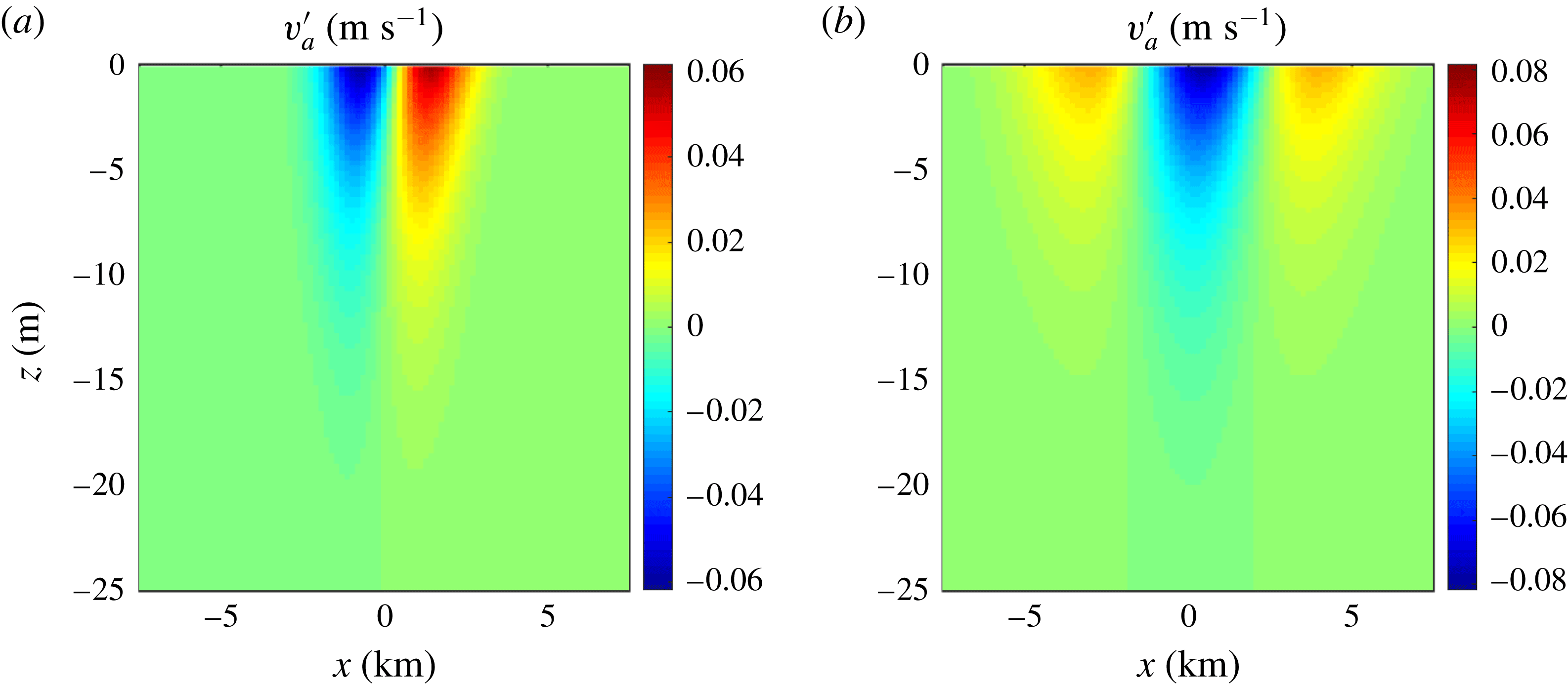
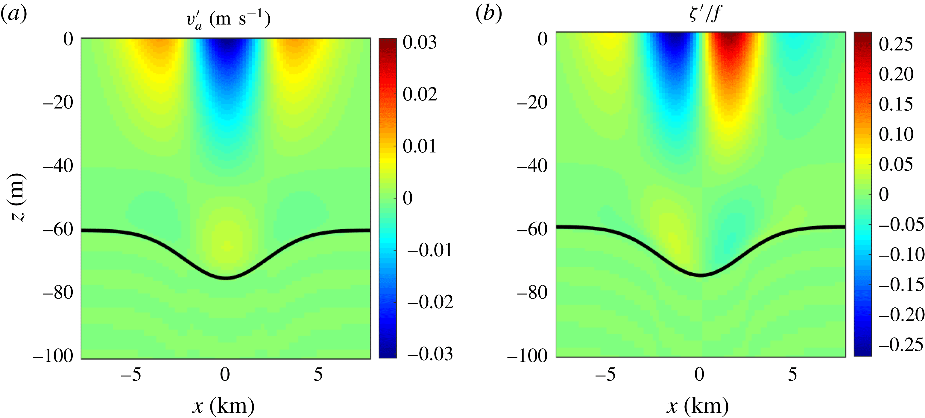
Stokes ageostrophic velocity anomaly
 $v_{a}^{\prime }=v_{1}(x,z)$
(after subtracting the far-field velocity, which in this case is an anti-Stokes flow,
 $-v_{st}(z)$
) for conservative flow with Stokes drift,
 $\unicode[STIX]{x1D703}_{st}=\unicode[STIX]{x03C0}/4$
, and no vertical mixing: a 2-D front (a) and a dense filament (b). These
 $v_{1}$
fields accompany the corresponding
 $b$
and
 $v_{g}$
fields in figure 1, but here the plotted vertical range is compressed. Notice the reduced vertical range for
 $v_{1}$
compared to the TTW
 $v_{a}$
in figure 2.

Thus, there is no flow in the cross-frontal plane associated with the submesoscale front or filament, only the anti-Stokes flow,
 $u=-u_{st}(z)$
with
 $w=0$
. The along-front ageostrophic flow is
 $v_{a}=-v_{st}+v_{1}$
, and the latter is confined to the submesoscale region, with a near-field anomaly,
 $v_{a}^{\prime }=v_{1}$
, that is forced by the combination of
 $\unicode[STIX]{x1D701}_{g}$
and
 $\unicode[STIX]{x2202}_{z}v_{st}$
in (5.5), both of which have a single sign in
 $z$
, leading to a surface-intensified structure in
 $v_{1}$
. It can be solved for by integrating upward from
 $v_{1}=0$
at depth, along tilting characteristics in the
 $(x,z)$
plane defined by
 $\text{d}X/\text{d}Z=(\unicode[STIX]{x2202}_{z}v_{st})/f$
, which is positive when
 $f>0$
and
 $\unicode[STIX]{x1D703}_{st}\unicode[STIX]{x1D716}(0,\unicode[STIX]{x03C0})$
, as in figure 8. This tilting is itself a
 $O(\widehat{\unicode[STIX]{x1D700}})$
modification to the vertical alignment in
 $v(x,z)$
that would occur without the second left-hand side term in (5.5). In this example, the horizontal displacement of a characteristic line is
 ${\sim}U_{st}/f\approx 1$
km at the surface. Because the forcing in (5.5) is
 $\propto \unicode[STIX]{x2202}_{x}v_{g}$
, with a horizontally uniform multiplier,
 $v_{1}$
has an opposite
 $x$
-symmetry compared to
 $v_{g}$
; i.e. for a front with an even-symmetric monopole in
 $v_{g}$
,
 $v_{1}$
is an odd-symmetric dipole and with
 $v_{g}$
/odd/dipole and
 $v_{1}$
/even/tripole structures, respectively, for a dense filament (cf. figure 1). Because
 $v_{st}\propto \sin [\unicode[STIX]{x1D703}_{st}]$
, the sign of the right-hand side forcing and of
 $v_{1}$
itself change with a reversal of the wave direction, and the sign of the characteristic tilt also changes. Thus, it is only the down-axis component of
 $\boldsymbol{u}_{st}$
that matters for
 $v_{1}$
, and with a stronger
 $v_{st}$
there is a greater phase tilt in
 $v_{1}$
. In this particular example, both
 $\boldsymbol{u}_{st}$
and
 $v_{1}$
are nearly as large as
 $v_{g}$
. Because of the opposite
 $x$
-symmetry of
 $v_{1}$
relative to
 $v_{g}$
, the conservative Stokes flow primarily contributes to a shape change for the geostrophic submesoscale current.
The spatial structure of these SCFT solutions is similar to those for the adjustment problem (McWilliams & Fox-Kemper Reference McWilliams and Fox-Kemper2013, figures 3 and 5): the
 $x$
-symmetry reversal between
 $v_{g}$
and
 $v_{1}$
and the tilting of the characteristic lines (at
 $O(\unicode[STIX]{x1D700})$
there). The differences are that in the adjustment problem
 $v_{1}$
, its vertical extent and its characteristic horizontal displacement are all larger, as explained following (5.6). A more subtle difference is that the adjustment solution has a sign reversal in
 $z$
underneath the surface layer where
 $v_{st}\neq 0$
, compared to the single-sign structure for the SCFT solution that is vertically confined to this surface layer.
For the ageostrophic vorticity fields, only the near-field response contributes, with
 $\unicode[STIX]{x1D701}_{a}=\unicode[STIX]{x2202}_{x}v_{1}$
. The patterns are again approximately in
 $x$
-quadrature with the geostrophic
 $\unicode[STIX]{x1D701}_{g}$
(figure 9). A front has a geostrophic dipole in
 $\unicode[STIX]{x1D701}$
and a Stokes-induced tripole with a strong central cyclonic band, while a dense filament has a geostrophic tripole with a strong central cyclonic band with a Stokes-induced quadrupole that is dominated by a central dipole. The magnitudes of
 $\unicode[STIX]{x1D701}_{a}$
are large, nearly as large as for
 $\unicode[STIX]{x1D701}_{g}$
in this
 $\widehat{\unicode[STIX]{x1D700}}\approx 1$
solution. The
 $\unicode[STIX]{x1D701}_{a}$
magnitude is relatively magnified in a front because of its smaller
 $\ell$
value chosen in § 3.
Stokes ageostrophic vorticity,
 $\unicode[STIX]{x1D701}_{a}=\unicode[STIX]{x2202}_{x}v_{1}$
, normalized by
 $f$
, for a front (a) and a dense filament (b) with
 $\unicode[STIX]{x1D703}_{st}=\unicode[STIX]{x03C0}/4$
and
 $\unicode[STIX]{x1D708}_{v}=\unicode[STIX]{x1D705}_{v}=0$
. These fields are calculated from the
 $v_{a}^{\prime }$
fields in figure 8.

Because
 $u_{a}^{\prime }=0$
and
 $w=0$
in this conservative SCFT solution, there is no frontogenetic tendency,
 ${\mathcal{T}}^{b}={\mathcal{T}}^{\boldsymbol{u}}=0$
(§ 2.4), consistent with it being a steady solution. For the same reason, there is no net buoyancy flux in either the cross-front horizontal or vertical directions (i.e.
 $BF_{v}=BF_{h}=0$
, as defined in equation (3.8) of SF1), nor any buoyancy flux in the along-front direction because of the 2-D assumption (§ 3), nor any Ekman pumping (i.e.
 $\unicode[STIX]{x2202}_{x}T_{a}^{x}=0$
, as defined in equation (4.1) of SF1).
As a final remark for this Stokes frontal solution, it is inconsistent to make a linear approximation and neglect the ageostrophic advection terms in the horizontal momentum balance in (2.4) or (2.11). This is because the linear solution for
 $u_{a}^{\prime }$
has a neglected
 $y$
-momentum horizontal advection term
 $-u\unicode[STIX]{x2202}_{x}v$
as large as its vortex force term,
 $-u_{st}\unicode[STIX]{x1D701}$
, which cancel each other in the nonlinear solution described above, and this statement is independent of
 $Ro$
. This in turn would modify (5.5) if advection were neglected. In the non-conservative
 $\unicode[STIX]{x1D708}_{v}\neq 0$
solutions of §§ 4 and 5.3.2–5.4, the nonlinear corrections are
 $O(Ro)$
, hence linear solutions are approximately valid when
 $Ro\ll 1$
.
5.3 Stokes secondary circulation with turbulent mixing
Now consider the three-way interaction of a submesoscale buoyancy gradient, Stokes drift and vertical mixing by boundary-layer turbulence. This is done in three parts within this subsection: first, secondary circulation for cases with weak mixing as an extension of the conservative SCFT solutions in § 5.2; second, secondary circulation with strong mixing; and third, frontogenetic tendency and buoyancy flux for both weak and strong mixing. The further addition of surface wind stress and Ekman currents in wind–wave equilibrium is examined in § 5.4.
5.3.1 Weak mixing
The preceding conservative SCFT Stokes solution can be built upon with small but finite
 $\unicode[STIX]{x1D708}_{v}$
and
 $\unicode[STIX]{x1D705}_{v}$
. The appropriate extended WEC solution form with specified
 $b$
and
 $\boldsymbol{u}_{st}$
is the following (cf. (5.1)):
 $$\begin{eqnarray}\displaystyle \left.\begin{array}{@{}c@{}}\displaystyle u=-u_{st}(z)+u_{\unicode[STIX]{x1D708}\infty }^{\dagger }(z)+u_{\unicode[STIX]{x1D708}}^{\prime }(x,z),\quad w=w_{\unicode[STIX]{x1D708}}^{\prime }(x,z),\\ \displaystyle v=v_{g}(x,z)-v_{st}(z)+v_{1}(x,z)+v_{\unicode[STIX]{x1D708}\infty }^{\dagger }(z)+v_{\unicode[STIX]{x1D708}}^{\prime }(x,z).\end{array}\right\} & & \displaystyle\end{eqnarray}$$
In this section,
 $\unicode[STIX]{x1D749}$
is kept at zero, while the magnitudes of
 $\unicode[STIX]{x1D708}_{v}=\unicode[STIX]{x1D705}_{v}$
are allowed to vary from small to the values implied in (3.7). As remarked in § 5.1, the view is taken that the turbulent mixing coefficients are independent control parameters as a means of exposing their effects on the TTW and WEC secondary circulations; of course, this is not the wind-driven equilibrium situation, which is examined in § 5.4.
The conservative ageostrophic correction component
 $v_{1}$
is the same as in § 5.2, and it is the solution to the PDE (5.5). The new horizontal components enabled by mixing are
 $\boldsymbol{u}_{\unicode[STIX]{x1D708}\infty }^{\dagger }$
and
 $\boldsymbol{u}_{\unicode[STIX]{x1D708}}^{\prime }$
. The former is the deviation from the anti-Stokes component in far-field Stokes–Ekman solution
 $\boldsymbol{u}_{\infty }(z)$
examined in § 5.1 and, with constant
 $\unicode[STIX]{x1D708}_{v}$
, in appendix A, with the velocity symbol
 $\boldsymbol{u}$
; both of these other solutions are equal to the sum of
 $-\boldsymbol{u}_{st}+\boldsymbol{u}_{\unicode[STIX]{x1D708}\infty }^{\dagger }$
in (5.7) and in the rest of this section. Defining
 $h_{ek}=\sqrt{2\unicode[STIX]{x1D708}_{v0}/f}$
with
 $\unicode[STIX]{x1D708}_{v0}$
a characteristic near-surface value of
 $\unicode[STIX]{x1D708}_{v}$
, a scaling estimate of the relative magnitude of
 $\boldsymbol{u}_{\unicode[STIX]{x1D708}\infty }^{\dagger }$
comes from the surface boundary condition of no stress by cancelling the Stokes-drift shear,
 $\unicode[STIX]{x2202}_{z}\boldsymbol{u}_{st}$
:
 $$\begin{eqnarray}\displaystyle \unicode[STIX]{x1D6FE}_{\infty }=\frac{h_{ek}}{h_{st}}\sim \frac{V_{\unicode[STIX]{x1D708}\infty }^{\dagger }}{U_{st}}, & & \displaystyle\end{eqnarray}$$
with
 $\unicode[STIX]{x1D6FE}_{\infty }\ll 1$
in the small-
 $\unicode[STIX]{x1D708}_{v}$
limit.
 $\boldsymbol{u}_{\unicode[STIX]{x1D708}\infty }^{\dagger }(z)$
is non-zero only over a depth
 ${\sim}h_{ek}$
near the surface (cf. (A 1)).
The other mixing-induced component
 $\boldsymbol{u}_{\unicode[STIX]{x1D708}}^{\prime }$
is confined to the horizontal neighbourhood of the submesoscale
 $v_{g}$
structure. Again, using the surface boundary condition of no stress (by cancelling the conservative ageostrophic Stokes shear
 $\unicode[STIX]{x2202}_{z}v_{1}$
), its relative magnitude is estimated as
 $$\begin{eqnarray}\displaystyle \unicode[STIX]{x1D6FE}^{\prime }=\widehat{\unicode[STIX]{x1D700}}\frac{h_{ek}}{h_{st}}\sim \frac{V_{\unicode[STIX]{x1D708}}^{\prime }}{V_{g}}, & & \displaystyle\end{eqnarray}$$
also with
 $\unicode[STIX]{x1D6FE}^{\prime }\ll 1$
in the small-
 $\unicode[STIX]{x1D708}_{v}$
limit. An accompanying assumption here is that the surface geostrophic shear,
 $\unicode[STIX]{x2202}_{z}v_{g}$
, is not larger than
 $\unicode[STIX]{x2202}_{z}v_{1}$
, i.e. that
 $h_{st}/(h\widehat{\unicode[STIX]{x1D700}})=1/\unicode[STIX]{x1D700}$
is not large (cf. (5.2)); otherwise, the appropriate value for
 $\unicode[STIX]{x1D6FE}^{\prime }$
would be
 $h_{ek}/h\ll 1$
. The relative size of these near- and far-field diffusive components is
 $$\begin{eqnarray}\displaystyle \frac{V_{\unicode[STIX]{x1D708}}^{\prime }}{V_{\unicode[STIX]{x1D708}\infty }^{\dagger }}\sim Ro. & & \displaystyle\end{eqnarray}$$
Consistent with these scalings, the dimensional problem for
 $\boldsymbol{u}_{\unicode[STIX]{x1D708}}^{\prime }$
, to leading order in small
 $\unicode[STIX]{x1D6FE}_{\infty }$
,
 $\unicode[STIX]{x1D6FE}^{\prime }$
and
 $h_{st}/h$
, is the following:
 $$\begin{eqnarray}\displaystyle \left.\begin{array}{@{}c@{}}\displaystyle -fv_{\unicode[STIX]{x1D708}}^{\prime }-\unicode[STIX]{x2202}_{z}(\unicode[STIX]{x1D708}_{v}\unicode[STIX]{x2202}_{z}u_{\unicode[STIX]{x1D708}}^{\prime })=0,\\ \displaystyle fu_{\unicode[STIX]{x1D708}}^{\prime }-\unicode[STIX]{x2202}_{z}(\unicode[STIX]{x1D708}_{v}\unicode[STIX]{x2202}_{z}v_{\unicode[STIX]{x1D708}}^{\prime })=-(u_{\unicode[STIX]{x1D708}}^{\prime }+u_{\unicode[STIX]{x1D708}\infty }^{\dagger })\unicode[STIX]{x2202}_{x}(v_{g}+v_{1}),\\ \displaystyle \unicode[STIX]{x2202}_{z}u_{\unicode[STIX]{x1D708}}^{\prime }=0\quad \text{and}\quad \unicode[STIX]{x2202}_{z}v_{\unicode[STIX]{x1D708}}^{\prime }=-\unicode[STIX]{x2202}_{z}(v_{g}+v_{1})\quad \text{at}~z=0,\\ \displaystyle \boldsymbol{u}_{\unicode[STIX]{x1D708}}^{\prime }\rightarrow 0\quad \text{as}~z\rightarrow -\infty .\end{array}\right\} & & \displaystyle\end{eqnarray}$$
Here
 $\boldsymbol{u}_{\unicode[STIX]{x1D708}}^{\prime }$
also is non-zero only over a depth
 ${\sim}h_{ek}$
near the surface. In addition to the surface boundary condition forcing at leading order, the two right-hand side terms in the
 $y$
-momentum equation have estimated magnitudes of order
 $Ro$
and unity, respectively, relative to the Ekman operator on the left-hand side (n.b. (5.10)); both terms arise from the nonlinear horizontal advection term,
 $-u\unicode[STIX]{x2202}_{x}v$
.
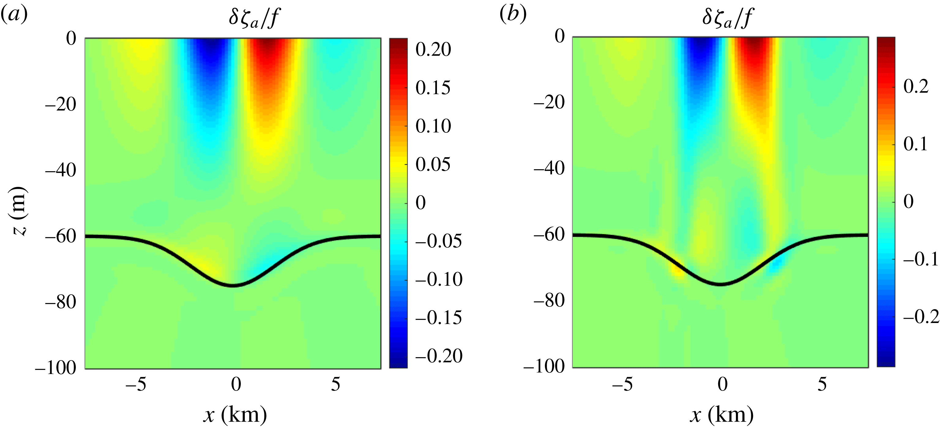
The accompanying equation for
 $w_{\unicode[STIX]{x1D708}}^{\prime }$
is 2-D continuity,
 $$\begin{eqnarray}\displaystyle \unicode[STIX]{x2202}_{x}u_{\unicode[STIX]{x1D708}}^{\prime }+\unicode[STIX]{x2202}_{z}w_{\unicode[STIX]{x1D708}}^{\prime }=0, & & \displaystyle\end{eqnarray}$$
with
 $w_{\unicode[STIX]{x1D708}}^{\prime }=0$
at
 $z=0$
. When this is solved in the TTW +
 $\unicode[STIX]{x1D6FA}$
E framework (§ 2.3), the deep boundary condition of
 $w_{\unicode[STIX]{x1D708}}^{\prime }(-\,H)=0$
can also be enforced. With this
 $\unicode[STIX]{x1D6FA}$
E component,
 $w_{\unicode[STIX]{x1D708}}^{\prime }$
reaches its peak value at a depth
 ${\sim}h_{ek}$
, while it decreases to zero only over the whole boundary-layer depth
 ${\sim}h$
and is zero below.
Thus, for small
 $\unicode[STIX]{x1D708}_{v}$
, the asymptotic nonlinear ageostrophic solution (5.7) can be obtained from a sequence of linear boundary value problems: (5.5) for the conservative
 $v_{1}$
; (5.3) for the far-field Stokes–Ekman flow,
 $\boldsymbol{u}=-\boldsymbol{u}_{st}+\boldsymbol{u}_{\unicode[STIX]{x1D708}\infty }^{\dagger }$
; and (5.11), (5.12) for the diffusive correction to the secondary circulation,
 $(\boldsymbol{u}_{\unicode[STIX]{x1D708}}^{\prime },w_{\unicode[STIX]{x1D708}}^{\prime })$
. This asymptotic partitioning provides a conceptual framework for distinguishing the varying influences on the SCFT circulation of the submesoscale buoyancy anomaly, the waves’ Stokes drift and the vertical mixing.
Stokes-induced ageostrophic vorticity (a) and vertical velocity (b) for a dense filament with
 $\unicode[STIX]{x1D703}_{st}=\unicode[STIX]{x03C0}/4$
and weak vertical mixing (i.e.
 $(\unicode[STIX]{x1D708}_{v},\unicode[STIX]{x1D705}_{v})$
are
 $1/64$
times the values implied by (3.7), with a spatial maximum value of
 $7\times 10^{-4}~\text{m}^{2}~\text{s}^{-1}$
). The boundary layer depth
 $z=-h(x)$
is indicated by the thick black line on the
 $w$
plot. This is a fully nonlinear SCFT solution.

The same as figure 10 except for a linear SCFT solution. Notice the expanded colour bar ranges.

An actual TTW +
 $\unicode[STIX]{x1D6FA}$
E solution for weak
 $(\unicode[STIX]{x1D708}_{v},\unicode[STIX]{x1D705}_{v})$
is shown in figure 10. As mentioned in § 4, most of the results are presented here only for a dense filament configuration, leaving the companion frontal results to be inferred. The
 $\unicode[STIX]{x1D701}_{a}$
field (hence also
 $v_{a}^{\prime }$
) is quite similar to the conservative Stokes solution
 $\unicode[STIX]{x1D701}_{1}$
in figure 9(b) but a bit weaker. The reason is the same as for
 $\unicode[STIX]{x1D701}_{a}$
acting to weaken
 $\unicode[STIX]{x1D701}_{g}$
in a TTW solution (§ 4): the mixing-induced correction partly cancels the primary flow that engenders it, in this case by cancelling the surface shear,
 $-\unicode[STIX]{x2202}_{z}v_{1}(0)$
. The corresponding
 $w$
field implies a single primary overturning cell, with upwelling on the cyclonic side (figure 1
d). The magnitude is only somewhat weaker than the corresponding
 $w$
in the TTW solution with full mixing strength but without WEC (figure 3). This secondary circulation in the cross-axis plane is entirely due to the mixing, because the wholly conservative solution has
 $w=0$
(§ 5.2). In
 $\unicode[STIX]{x1D6F7}$
the pattern is a tripole with a dominant central cell. All of these ageostrophic circulation patterns have approximately opposite
 $x$
-symmetries compared to the TTW patterns in figures 2 and 3, consistent with the symmetries of the conservative Stokes solution in § 5.2, even though the combination of the
 $\unicode[STIX]{x1D708}_{v}$
and
 $\boldsymbol{u}_{st}$
influences on
 $\boldsymbol{u}_{a}$
lacks this exact symmetry.
The same as figure 10 except for different
 $\boldsymbol{u}_{st}$
directions:
 $\unicode[STIX]{x1D703}_{st}=0$
(a,b),
 $\unicode[STIX]{x03C0}/2$
(c,d) and
 $3\unicode[STIX]{x03C0}/4$
(e,f). The intermediate direction
 $\unicode[STIX]{x1D703}_{st}=\unicode[STIX]{x03C0}/4$
is shown in figure 10. These show that the along-front ageostrophic flow
 $v_{a}^{\prime }$
is strongest when the waves are aligned with the filament axis and that the cross-front overturning circulation
 $\unicode[STIX]{x1D6F7}^{\prime }$
is strongest when the waves are across the axis (n.b. the small colour scales in a and d).

Because these solutions are for vertically varying eddy diffusivities, it is somewhat uncertain what value to take for
 $h_{ek}$
in comparison with the estimates in (5.8), (5.9), especially near the surface where
 $\unicode[STIX]{x1D708}_{v}(z)$
becomes small in addition to
 $h_{ek}$
being small. Nevertheless, the estimates from
 $\unicode[STIX]{x1D6FE}^{\prime }$
in (5.9) are
 $$\begin{eqnarray}\displaystyle V_{\unicode[STIX]{x1D708}}^{\prime }\sim \frac{h_{ek}U_{st}V_{g}}{h_{st}f\ell },\quad \unicode[STIX]{x1D6F7}_{\unicode[STIX]{x1D708}}^{\prime }\sim \frac{\unicode[STIX]{x1D708}_{v}U_{st}V_{g}}{h_{st}f^{2}\ell },\quad W_{\unicode[STIX]{x1D708}}^{\prime }\sim \frac{\unicode[STIX]{x1D708}_{v}U_{st}V_{g}}{h_{st}f^{2}\ell ^{2}}, & & \displaystyle\end{eqnarray}$$
and these are roughly consistent with the solutions shown here. Extrapolating these balances to larger
 $\unicode[STIX]{x1D708}_{v}$
values, when
 $h_{ek}\sim h_{st}$
, the estimates instead become
 $$\begin{eqnarray}\displaystyle V_{\unicode[STIX]{x1D708}}^{\prime }\sim \widehat{\unicode[STIX]{x1D700}}V_{g},\quad \unicode[STIX]{x1D6F7}_{\unicode[STIX]{x1D708}}^{\prime }\sim \widehat{\unicode[STIX]{x1D700}}hV_{g},\quad W_{\unicode[STIX]{x1D708}}^{\prime }\sim \frac{h\widehat{\unicode[STIX]{x1D700}}V_{g}}{\ell }, & & \displaystyle\end{eqnarray}$$
where
 $\widehat{\unicode[STIX]{x1D700}}$
is defined in (5.6). (For even larger
 $h_{ek}$
, see (5.18) in § 5.3.2.)
Figure 10 is for a fully nonlinear SCFT solution. Its linear counterpart, neglecting all ageostrophic advection (hence all advection in a 2-D configuration), is figure 11. As explained for the fully conservative Stokes circulation in § 5.2, the linear SCFT solution provides an overestimate of the ageostrophic circulation, at least for small
 $(\unicode[STIX]{x1D708}_{v},\unicode[STIX]{x1D705}_{v})$
, because it does not account for the cancellation between the vortex force and horizontal advection that arises when
 $\boldsymbol{u}_{a}\approx -\boldsymbol{u}_{st}$
(e.g. as in (5.1) and (5.7)).
The same as figure 10 except for different vertical mixing magnitudes: with
 $(\unicode[STIX]{x1D708}_{v},\unicode[STIX]{x1D705}_{v})$
reduced by only a factor of
 $1/8$
(i.e.
 $\unicode[STIX]{x1D708}_{v}=\unicode[STIX]{x1D705}_{v}=6\times 10^{-3}~\text{m}^{2}~\text{s}^{-1}$
; a,b) and with the full strength implied by the parameters in (3.7),
 $\unicode[STIX]{x1D708}_{v}=\unicode[STIX]{x1D705}_{v}=5\times 10^{-2}~\text{m}^{2}~\text{s}^{-1}$
(c,d). These are fully nonlinear SCFT solutions. The depth range in (c) is increased to 100 m, for more direct comparison with the TTW solution in figure 4(a). For other comparisons, the very small mixing solution is in figure 10, and the no-mixing solution is in figure 9(b) for
 $\unicode[STIX]{x1D701}_{a}$
, with its associated
 $w=0$
.

The
 $\boldsymbol{u}_{a}$
directional dependency on
 $\boldsymbol{u}_{st}$
is illustrated in figure 12. Compared to the direction
 $\unicode[STIX]{x1D703}_{st}=\unicode[STIX]{x03C0}/4$
in figure 10, the cross-axis overturning circulation is stronger for cross-axis waves (
 $\unicode[STIX]{x1D703}_{st}=0.0$
) and weaker for along-axis waves (
 $\unicode[STIX]{x1D703}_{st}=\unicode[STIX]{x03C0}/2$
). The opposite relations hold for the ageostrophic vorticity, echoing the
 $\unicode[STIX]{x1D703}_{st}$
dependency in the conservative Stokes solution (5.5). This indicates a rough
 $\sin [\unicode[STIX]{x1D703}_{st}]$
dependency for
 $v_{a}^{\prime }$
and
 $\cos [\unicode[STIX]{x1D703}_{st}]$
dependency for
 $u_{a}^{\prime }$
, which are also passed on to their derivative fields (i.e.
 $\unicode[STIX]{x1D701}_{a}$
for the former and
 $(\unicode[STIX]{x1D6F7}_{a},w)$
for the latter). As therefore expected,
 $\unicode[STIX]{x1D701}_{a}$
and
 $w$
for
 $\unicode[STIX]{x1D703}_{st}=3\unicode[STIX]{x03C0}/4$
are approximately, but not exactly, the even and odd reflections of the
 $\unicode[STIX]{x1D703}_{st}=\unicode[STIX]{x03C0}/4$
fields relative to the centre at
 $x=0$
. There is an exact sign-reversal symmetry for all of the ageostrophic fields for
 $\unicode[STIX]{x1D703}_{st}\leftrightarrow \unicode[STIX]{x1D703}_{st}\pm \unicode[STIX]{x03C0}$
. Similar angle dependencies are found in the linear SCFT solutions, but again the ageostrophic secondary circulation magnitudes are larger than in the nonlinear solutions for the reason stated in relation to figure 10.
In summary, weak vertical mixing supports a secondary circulation in the cross-frontal plane whose shape is controlled primarily by the Stokes vortex force.
5.3.2 Strong mixing
A sequence of nonlinear SCFT solutions with increasing vertical mixing strength is shown in figure 13 for
 $\unicode[STIX]{x1D703}_{st}=\unicode[STIX]{x03C0}/4$
. As
 $\unicode[STIX]{x1D708}_{v}$
increases from its very small value in figure 10,
 $\unicode[STIX]{x1D701}_{a}$
at first strengthens slightly, then it also begins to show aspects of the spatial pattern of the nonlinear TTW solution seen in figure 4. For
 $w$
the pattern shift toward a stronger, dominant single downwelling jet begins even at intermediate mixing values, and by full mixing strength it becomes quite similar to the TTW pattern although slightly weaker. For strong mixing the primary pattern for
 $\unicode[STIX]{x1D701}_{a}$
becomes a monopole in the horizontal direction and for
 $w$
a tripole, whereas for small mixing the respective patterns are both dipoles.
Thus, the WEC secondary circulation is in competition with the TTW secondary circulation mediated by the vertical mixing strength. In the TTW cases the secondary circulation decreases linearly with
 $\unicode[STIX]{x1D708}_{v}$
, consistent with its scaling dependency,
 $$\begin{eqnarray}\displaystyle \unicode[STIX]{x1D6F7}_{ttw}\sim \frac{\unicode[STIX]{x1D708}_{v}V_{g}}{fh}\quad \text{and}\quad V_{ttw}\sim \frac{\unicode[STIX]{x1D708}_{v}V_{g}}{fh^{2}}=Ek_{h}V_{g}, & & \displaystyle\end{eqnarray}$$
with
 $Ek_{h}=\unicode[STIX]{x1D708}_{v}/fh^{2}$
an Ekman number for a surface layer of depth
 $h$
(SF1, equation (4.6)). In contrast, the Stokes ageostrophic circulation components decrease only moderately with
 $\unicode[STIX]{x1D708}_{v}$
, thus becoming dominant for small
 $\unicode[STIX]{x1D708}_{v}$
. Recall that the TTW SCFT solution has almost no directional dependency (even when
 $\unicode[STIX]{x1D749}\neq 0$
except for very large
 $U_{atm}$
), so its competition with the WEC solution will also have little directional dependency.
Normalized ageostrophic vorticity differences,
 $\unicode[STIX]{x1D6FF}\unicode[STIX]{x1D701}_{a}/f$
, between WEC and TTW solutions for full-strength vertical mixing and
 $\unicode[STIX]{x1D703}_{st}=\unicode[STIX]{x03C0}/4$
for a dense filament: (a) linear solutions with figure 3(a) subtracted from the WEC solution and (b) nonlinear solutions with figure 4(a) subtracted out. These patterns are similar to the conservative Stokes solution with
 $\unicode[STIX]{x1D708}_{v}=\unicode[STIX]{x1D705}_{v}=0$
(figure 8
b), albeit here reduced in amplitude, showing that the WEC effects are similar even when the total
 $\unicode[STIX]{x1D701}_{a}$
field is dominated by the TTW effects (cf. figures 13
c for WEC and 4
a for TTW only).

In analogy with the previous solution forms (i.e. the conservative Stokes solution form (5.1), the far-field Stokes–Ekman form (5.3), and the weak mixing form (5.7)), the large mixing solution form is
 $$\begin{eqnarray}\displaystyle \left.\begin{array}{@{}c@{}}\displaystyle \boldsymbol{u}(x,z)=v_{g}(x,z)\widehat{\boldsymbol{y}}-\boldsymbol{u}_{st}(z)+\boldsymbol{u}_{\unicode[STIX]{x1D708}\infty }^{\dagger }(z)+\boldsymbol{u}_{ttw}(x,z)+\boldsymbol{u}^{\prime }(x,z),\\ \displaystyle w(x,z)=w_{ttw}(x,z)+w^{\prime }(x,z).\end{array}\right\} & & \displaystyle\end{eqnarray}$$
The first term in
 $\boldsymbol{u}$
is the geostrophic along-axis flow, the second and third terms are the far-field Stokes–Ekman flow (e.g. appendix A), the fourth term is the TTW ageostrophic flow without WEC influences (§ 4) and the final term is the WEC correction in the near field. Only the latter two terms have an associated near-field overturning circulation
 $w$
. With the knowledge from the solutions in figures 13 and 14 that
 $(\boldsymbol{u}^{\prime },w^{\prime })$
are small corrections to
 $(\boldsymbol{u}_{ttw},w_{ttw})$
when the vertical mixing is strong, that
 $v_{g}$
and
 $\boldsymbol{u}_{st}$
are the strongest horizontal flows, and that
 $k_{st}h\gg 1$
, a simplified approximate system is proposed for
 $(\boldsymbol{u}^{\prime },w^{\prime })$
:
 $$\begin{eqnarray}\displaystyle \left.\begin{array}{@{}c@{}}\displaystyle -fv^{\prime }-\unicode[STIX]{x2202}_{z}(\unicode[STIX]{x1D708}_{v}\unicode[STIX]{x2202}_{z}u^{\prime })=\int _{-H}^{z}(\unicode[STIX]{x2202}_{z}v_{st})\unicode[STIX]{x1D701}_{g}\,\text{d}z,\\ \displaystyle fu^{\prime }-\unicode[STIX]{x2202}_{z}(\unicode[STIX]{x1D708}_{v}\unicode[STIX]{x2202}_{z}v^{\prime })=-u_{st}\unicode[STIX]{x1D701}_{g},\\ \displaystyle \unicode[STIX]{x2202}_{x}u^{\prime }+\unicode[STIX]{x2202}_{z}w^{\prime }=0,\\ \displaystyle \unicode[STIX]{x2202}_{z}u^{\prime }=\unicode[STIX]{x2202}_{z}v^{\prime }=0\quad \text{at}~z=0,\\ \displaystyle \boldsymbol{u}^{\prime }\rightarrow 0\quad \text{as}~z\rightarrow -\infty ,\\ \displaystyle w^{\prime }=0\quad \text{at}~z=0.\end{array}\right\} & & \displaystyle\end{eqnarray}$$
This is an Ekman-like, linear ordinary differential equation (ODE) system (i.e. with only a parametric
 $x$
dependency given
 $v_{g}(x,z)$
and
 $\boldsymbol{u}_{st}(z)$
) with zero surface stress that is forced by the leading-order 2-D vortex force terms from (2.11). Ageostrophic advection is neglected either because its leading-order effects are incorporated in the TTW balance or because all other quadratic terms are small as the far-field velocity,
 $-\boldsymbol{u}_{st}(z)+\boldsymbol{u}_{\unicode[STIX]{x1D708}\infty }^{\dagger }$
, and
 $\boldsymbol{u}^{\prime }$
are both small compared to the right-hand side horizontal forces in (5.17). The success of this approximation is demonstrated in figure 15 for
 $v_{a}^{\prime }$
and
 $\unicode[STIX]{x1D701}_{a}$
by its similarity with the difference between full TTW +
 $\unicode[STIX]{x1D6FA}$
E SCFT solutions with and without WEC in figure 14. The fact of its similarity to both the linear and nonlinear solutions further supports the approximation of neglecting the ageostrophic advective effects in (5.17).
Thus, the ageostrophic WEC secondary circulation around a front here is driven by the product of the frontal geostrophic shear
 $\unicode[STIX]{x1D701}_{g}$
and the Stokes drift
 $\boldsymbol{u}_{st}$
through the Stokes vortex force; this is analogous to the conservative secondary circulation
 $v_{1}$
in § 5.2 (esp. figure 8), except that now the
 $v_{a}^{\prime }(x,z)$
shape is different because of the strong vertical mixing.
Ageostrophic velocity,
 $v_{a}^{\prime }$
(a), and normalized ageostrophic vorticity,
 $\unicode[STIX]{x1D701}^{\prime }/f$
(b), in the solution to the simplified vortex force system (5.17) for full-strength vertical mixing and
 $\unicode[STIX]{x1D703}_{st}=\unicode[STIX]{x03C0}/4$
for a dense filament with WEC. Notice the resemblance of
 $\unicode[STIX]{x1D701}^{\prime }$
to the
 $\unicode[STIX]{x1D6FF}\unicode[STIX]{x1D701}_{a}/f$
in the full TTW +
 $\unicode[STIX]{x1D6FA}$
E solutions in figure 14, as well as of both fields to the conservative Stokes solution in figures 8(b) and 9(b), respectively, albeit here with a reduced magnitude due to the vertical mixing.

The simplified system (5.17) is incomplete, most obviously because of its insufficient vertical differential order to satisfy the lower boundary condition for
 $w^{\prime }$
in (5.17), as well as because of its lack of consideration of the buoyancy balance. It is a partial system in the same sense as the TTW subsystem (2.10) for
 $(\boldsymbol{u}_{T},w_{T})$
is incomplete without
 $(\boldsymbol{u}_{O},w_{O})$
from the
 $\unicode[STIX]{x1D6FA}$
E subsystem. Thus,
 $(\boldsymbol{u}^{\prime },w^{\prime })$
is identified with
 $(\boldsymbol{u}_{T},w_{T})$
, and requires an
 $\unicode[STIX]{x1D6FA}$
E completion; notice, however, that
 $\unicode[STIX]{x1D6FA}$
E only provides a modification to
 $u$
, not to
 $v$
, leaving
 $v^{\prime }$
from (5.17) at the total
 $v$
field. The
 $u^{\prime }$
solution from (5.17) is small in this situation with the standard case parameters in § 3, less than half the size of
 $v^{\prime }$
, so its associated
 $w^{\prime }$
and
 $\unicode[STIX]{x1D6F7}^{\prime }$
are also small, and its
 $\unicode[STIX]{x1D6FA}$
E correction fields are comparably small (not shown). This is consistent with the
 $\unicode[STIX]{x1D6FF}u$
,
 $\unicode[STIX]{x1D6FF}w$
and
 $\unicode[STIX]{x1D6FF}\unicode[STIX]{x1D6F7}$
companion fields (not shown) being small as is the
 $\unicode[STIX]{x1D6FF}\unicode[STIX]{x1D701}_{a}$
WEC correction to the TTW solutions in figure 14.
From (5.17) a scaling estimate for the WEC correction
 $\boldsymbol{u}^{\prime }$
comes from the particular solution for the right-hand side interior forcing terms, viz.,
 $$\begin{eqnarray}\displaystyle V^{\prime }\sim \frac{\text{max}[1,Ek_{st}]}{1+Ek_{st}^{2}}\widehat{\unicode[STIX]{x1D700}}V_{g}\approx \frac{\widehat{\unicode[STIX]{x1D700}}V_{g}}{(1+Ek_{st}^{2})^{1/2}}. & & \displaystyle\end{eqnarray}$$
 $Ek_{st}$
is an Ekman number associated with the thin upper part of the surface layer where
 $\boldsymbol{u}_{st}$
is large and
 $\unicode[STIX]{x1D708}_{v}(h_{st})$
from (3.4) is relatively small compared to the interior of the layer (i.e.
 $h_{st}\ll h$
):
 $$\begin{eqnarray}\displaystyle Ek_{st}=\frac{\unicode[STIX]{x1D708}_{v}(h_{st})}{fh_{st}^{2}}. & & \displaystyle\end{eqnarray}$$
For full-strength mixing (i.e. with the parameters in (3.7)),
 $Ek_{st}>1$
, and
 $V^{\prime }$
is thus reduced from the conservative Stokes flow,
 $V_{1}$
in (5.6), by the denominator factor in (5.18). From (5.15), the relative size of the WEC correction to the TTW circulation is therefore
 $$\begin{eqnarray}\displaystyle \frac{V^{\prime }}{V_{ttw}}\sim \widehat{\unicode[STIX]{x1D700}}\frac{Ek_{h}}{(1+Ek_{st}^{2})^{1/2}}\approx \widehat{\unicode[STIX]{x1D700}}\frac{Ek_{h}}{Ek_{st}}. & & \displaystyle\end{eqnarray}$$
For the standard parameters in § 3,
 $\widehat{\unicode[STIX]{x1D700}}$
is slightly less than one, while the ratio of Ekman numbers is small.
Thus, the WEC correction to the TTW secondary circulation is modest with strong mixing, as shown above in the comparison between figures 4 and 13(c,d). Additionally, the WEC secondary circulation contribution
 $V^{\prime }$
weakens with increasing mixing strength, i.e. as
 $Ek_{st}$
increases. There is a similar reduction for the far-field Stokes–Ekman velocity with increasing
 $\unicode[STIX]{x1D708}_{v}$
(§ 5.1 and appendix A).
A comparison of (5.13), (5.14) and (5.18) for
 $\unicode[STIX]{x1D708}_{v}$
increasing from small to large values, shows that a common factor in the estimates for the cross-frontal ageostrophic velocity
 $V^{\prime }$
is
 $\widehat{\unicode[STIX]{x1D700}}V_{g}$
, with reduced values for
 $h_{ek}$
small and large compared to
 $h_{st}$
. The conservative Stokes estimate for the along-front ageostrophic velocity
 $V_{1}$
in (5.5) is the same
 $\widehat{\unicode[STIX]{x1D700}}V_{g}$
estimate.
5.3.3 Frontogenetic tendency and buoyancy flux
The linear TTW secondary circulation (§ 4) shows a positive
 ${\mathcal{T}}^{\boldsymbol{u}}$
in the centre of a dense filament in the upper
 ${\approx}$
20 m. It is due to a dominant contribution from
 ${\mathcal{T}}_{adv}^{\boldsymbol{u}}\approx -(\unicode[STIX]{x2202}_{x}u)^{2}(\unicode[STIX]{x2202}_{x}v_{g})>0$
, where
 $u$
is convergent near the surface and
 $\unicode[STIX]{x2202}_{x}v_{g}$
is cyclonic. (See SF1, figure 9e,f for linear solutions for a front and dense filament.) For the filament in figures 1 and 2, the maximum value is
 ${\mathcal{T}}^{\boldsymbol{u}}(0,0)\approx 2.5\times 10^{-13}~\text{s}^{-3}$
. Its vertical buoyancy flux,
 $$\begin{eqnarray}\displaystyle BF_{v}(z)=\int _{-L_{x}/2}^{L_{x}/2}wb\,\text{d}x, & & \displaystyle\end{eqnarray}$$
is positive with a peak value
 ${\approx}3\times 10^{-4}~\text{m}^{3}~\text{s}^{-3}$
at a depth of approximately 40 m (cf. SF1, figure 14a). This is a conversion of the available potential energy in the filament to its kinetic energy, as is typical of submesoscale frontogenetic flows in the surface layer; it is also a buoyancy restratification flux. These TTW diagnostic implications are confirmed in frontogenetic simulations of a 2-D dense filament evolution (McWilliams et al.
Reference McWilliams, Gula, Molemaker, Renault and Shchepetkin2015).
The conservative Stokes circulation in § 5.2 is an exact nonlinear steady state and thus has
 ${\mathcal{T}}^{\boldsymbol{u}}=0$
, with cancellation between
 ${\mathcal{T}}_{adv}^{\boldsymbol{u}}$
and
 ${\mathcal{T}}_{W}^{\boldsymbol{u}}$
. It has
 $BF_{v}=0$
because
 $w=0$
.
Total velocity-gradient frontogenetic tendency,
 ${\mathcal{T}}^{\boldsymbol{u}}$
from (2.17), for a dense filament in several cases with WEC: (a) nonlinear SCFT solution with
 $(\unicode[STIX]{x1D708}_{v},\unicode[STIX]{x1D705}_{v})$
reduced by a factor of 64 and
 $\unicode[STIX]{x1D703}_{st}=\unicode[STIX]{x03C0}/4$
; (b) the same as (a) except that
 $\unicode[STIX]{x1D703}_{st}=0$
; (c) the same as (a) except with full-strength vertical mixing and (d) the same as (a) except for a linear SCFT solution.

With vertical mixing the WEC flows in §§ 5.3.1 and 5.3.2 have both positive frontogenetic tendencies and positive vertical buoyancy fluxes. The
 ${\mathcal{T}}^{\boldsymbol{u}}(x,z)$
patterns are illustrated in figure 16 with nonlinear SCFT solutions for several different
 $\unicode[STIX]{x1D708}_{v}$
and
 $\unicode[STIX]{x1D703}_{st}$
values, as well as with a linear solution for one parameter set. The patterns are remarkably similar, with a dominant positive extremum at the filament centre near the surface. This is flanked by a weaker negative centre that is on the east side for
 $\unicode[STIX]{x1D703}_{st}$
directed eastward. For westward-oriented waves, the flanking negative
 ${\mathcal{T}}^{\boldsymbol{u}}$
is on the west side, and for
 $\unicode[STIX]{x1D703}_{st}\approx \pm \unicode[STIX]{x03C0}/2$
,
 ${\mathcal{T}}^{\boldsymbol{u}}$
is quite weak because the cross-frontal flow is weak (cf. figure 12
d). The magnitude of
 ${\mathcal{T}}^{\boldsymbol{u}}$
is only moderately dependent on
 $\unicode[STIX]{x1D708}_{v}$
and
 $\unicode[STIX]{x1D703}_{st}$
, and for full mixing (figure 16
c) its value is nearly the same as mentioned for TTW alone two paragraphs above. With small
 $\unicode[STIX]{x1D708}_{v}$
, the linear SCFT WEC solution (figure 16
d) overestimates
 ${\mathcal{T}}^{\boldsymbol{u}}$
(figure 16
a), because it also overestimates the ageostrophic flow (cf. figures 10 and 11).
These WEC velocity-gradient frontogenetic tendencies are dominated by the advective contributions. The contribution explicitly arising from the vortex force,
 ${\mathcal{T}}_{W}^{\boldsymbol{u}}$
in (2.17) and (3.2) is relatively much smaller (figure 17), even though
 $\boldsymbol{u}_{st}$
itself is not small compared to
 $\boldsymbol{u}_{g}$
; rather it is due to the spatial misalignment (i.e. different
 $x$
-symmetries) of the contributing factors in
 ${\mathcal{T}}_{W}^{\boldsymbol{u}}$
, relative to the better alignment in
 ${\mathcal{T}}_{adv}^{\boldsymbol{u}}$
. The different
 ${\mathcal{T}}_{W}^{\boldsymbol{u}}$
patterns seen for different
 $\unicode[STIX]{x1D703}_{st}$
values are due to alternative contributions from the first two terms in (3.2). Thus, WEC modifies
 ${\mathcal{T}}^{\boldsymbol{u}}$
mainly by modifying
 $\boldsymbol{u}_{a}$
rather than directly through the vortex force tendency
 ${\mathcal{T}}_{W}^{\boldsymbol{u}}$
. As anticipated at the end of § 2.4, there is a close correspondence between
 ${\mathcal{T}}^{\boldsymbol{u}}>0$
near the surface and
 $w<0$
in the boundary layer (e.g. figures 16
a and 10
b) because of control of the frontogenetic rate by surface convergence in the submesoscale regime.


As remarked in SF1, the convex vertical profile shape of
 $BF_{v}(z)>0$
is remarkably robust across different submesoscale buoyancy and wind-forcing configurations. The same is true for the WEC SCFT solutions presented here, and for full-strength mixing its profile is essentially the same as for a TTW solution with only approximately a 10 % enhancement in its maximum, up to a value of
 $3.4\times 10^{-4}~\text{m}^{3}~\text{s}^{-3}$
. For TTW solutions, its magnitude varies
 $\propto \unicode[STIX]{x1D708}_{v}$
(SF1, equation (4.18)); i.e. it decreases for weak mixing because the secondary circulation weakens. For WEC solutions,
 $BF_{v}$
also weakens as
 $\unicode[STIX]{x1D708}_{v}$
decreases, not because the secondary circulation weakens so much (e.g. figures 10–13), but because the
 $x$
-shape of
 $w$
shifts from a tripole into a dipole that is in quadrature with the
 $x$
-shape of
 $b$
.
In summary, whatever the combination of TTW and WEC influences with vertical mixing, the secondary circulation in the cross-frontal plane induces frontogenetic tendencies (especially for velocity gradient) and a restratifying vertical buoyancy flux.
5.4 Wind–wave equilibrium
Now WEC SCFT solutions are examined with the full set of wind, wave and vertical mixing parameter values in § 3 that correspond to a representative state of wind–wave equilibrium (WWE).
Ageostrophic vorticity,
 $\unicode[STIX]{x1D701}_{a}/f$
, in WWE for a dense filament with
 $\unicode[STIX]{x1D703}_{\unicode[STIX]{x1D70F}}=\unicode[STIX]{x03C0}/4$
: (a) with and (b) without WEC. These are from fully nonlinear SCFT solutions.

When
 $\unicode[STIX]{x1D749}\neq 0$
, there is a far-field Ekman circulation that also spans the submesoscale flow region. This, in principle, provides a directional dependence on
 $\unicode[STIX]{x1D703}_{\unicode[STIX]{x1D70F}}$
; however, with ageostrophic advection still neglected, this effect is quite weak compared to the mixing-driven TTW circulation in figure 2, except when
 $U_{atm}$
is much larger for the same
 $v_{g}$
strength (SF1, § 4). With nonlinear advection also included together with wind stress
 $\unicode[STIX]{x1D749}$
in its most favourable direction, the TTW secondary circulation is narrower and has much stronger peak
 $w$
and
 ${\mathcal{T}}^{\boldsymbol{u}}$
values. Also, there is significant dependency on
 $\unicode[STIX]{x1D703}_{\unicode[STIX]{x1D70F}}$
even with this value of
 $U_{atm}$
(SF1, § 6), where the strongest secondary circulation occurs through a reinforcing interaction between the wind-driven Ekman and TTW flows. Even with this favourably reinforcing orientation,
 $BF_{v}(z)$
is only modestly enhanced from its linear TTW answer (§ 5.3.3).
Vertical velocity,
 $w$
, in WWE for a dense filament with
 $\unicode[STIX]{x1D703}_{\unicode[STIX]{x1D70F}}=\unicode[STIX]{x03C0}/4$
: (a) with and (b) without WEC. These are from fully nonlinear SCFT solutions.

To summarize the primary nonlinear WWE result, WEC alters the SCFT answers quantitatively but not qualitatively. This is illustrated in figures 18–20 for the direction
 $\unicode[STIX]{x1D703}_{\unicode[STIX]{x1D70F}}=\unicode[STIX]{x1D703}_{st}=\unicode[STIX]{x03C0}/4$
, which is close to the orientation that makes
 $w$
largest. In each plot parallel results are shown from cases with and without WEC. A scan in
 $\unicode[STIX]{x1D703}$
is not made here because it would be largely redundant with the wind-only nonlinear SCFT solutions in SF1, § 6.
Both with WEC and without it, the patterns of
 $\unicode[STIX]{x1D701}_{a}$
and
 $w$
(figures 18 and 19) have primary anticyclonic vorticity and downwelling velocity on the west side of the filament when the wind and waves are toward the north-east. The vorticity is somewhat stronger, and
 $w$
is somewhat weaker with WEC, though both are large compared to solutions with weaker mixing or to the linear solutions with full-strength mixing (not shown here, but see SF1, § 4). The WEC patterns in both fields are somewhat wider. Overall, these ageostrophic flows are rather similar with and without WEC, but their differences (figure 20) are almost as large as the total fields. This shows that the magnitude of the WEC influence is much larger in this WWE case than in comparable cases without wind stress (figure 14). The horizontal widths in the difference patterns are noticeably smaller than in the total fields, indicating that WEC has a fine-scale, reshaping influence on the flow.
Differences between WEC and no-WEC SCFT solutions for a dense filament with
 $\unicode[STIX]{x1D703}_{\unicode[STIX]{x1D70F}}=\unicode[STIX]{x03C0}/4$
: (a)
 $\unicode[STIX]{x1D6FF}\unicode[STIX]{x1D701}_{a}/f$
and (b)
 $\unicode[STIX]{x1D6FF}w$
. They may be compared with the full solution fields in figures 18 and 19. These are from fully nonlinear SCFT solutions.

Frontogenetic tendency for velocity gradient,
 ${\mathcal{T}}^{\boldsymbol{u}}$
, in WWE for a dense filament with
 $\unicode[STIX]{x1D703}_{\unicode[STIX]{x1D70F}}=\unicode[STIX]{x03C0}/4$
: (a) with and (b) without WEC. These are from fully nonlinear SCFT solutions.

The corresponding velocity-gradient frontogenetic tendencies
 ${\mathcal{T}}^{\boldsymbol{u}}(x,z)$
are in figure 21. The pattern of strong frontogenesis in the upper west sector (for winds and waves with an eastward component) again occurs, as with the wave-only SCFT solutions in § 5.3.3, but with much enhanced magnitudes compared to the comparable nonlinear solution in figure 16(c). The WEC solution has a stronger peak magnitude in
 ${\mathcal{T}}^{\boldsymbol{u}}$
, and it does not extend as deep as in the solution without WEC; however, both patterns are qualitatively similar.
The vertical buoyancy flux profile
 $BF_{v}(z)$
(not shown) again has the familiar convex shape across the surface layer with only modest WWE WEC enhancements of its peak magnitude compared to TTW alone or with WEC added (§ 5.3.3); i.e. the WWE peak values here are 4.1 and
 $3.7\times 10^{-4}~\text{m}^{3}~\text{s}^{-3}$
with and without WEC.
6 Current effects on the waves (CEW)
A simplification in the problems considered above is the assumption that the currents have no effect on the waves, i.e. no CEW. This is briefly re-examined here from a theoretical perspective. A recent observational discussion is in Ardhuin et al. (Reference Ardhuin, Gille, Menemenlis, Rocha, Rascle, Chapron, Gula and Molemaker2017).
The CEW theoretical framework is the geometrical optics approximation for the wave evolution (also known as ray theory: Bühler Reference Bühler2009) due to refraction by the current shear. It prescribes the evolution of the wave properties along ray paths that are everywhere parallel to the group velocity
 $\boldsymbol{C}_{g}(\boldsymbol{x})$
; these properties include the horizontal wavenumber vector
 $\boldsymbol{k}=(k,l)$
, the frequency
 $\unicode[STIX]{x1D714}$
and the amplitude
 $a$
. Its underlying assumption is that the wave medium (i.e. the current) is slowly varying in space and time compared to the wavelength,
 $\unicode[STIX]{x1D706}=2\unicode[STIX]{x03C0}/K$
, where
 $K^{2}=k^{2}+l^{2}$
, and period,
 $P=2\unicode[STIX]{x03C0}/\unicode[STIX]{x1D714}$
. In addition to the 2-D assumption in this paper (§ 3), further simplifying assumptions are that the waves are not influenced by the vertical shear of the current (hence only the surface velocity
 $\boldsymbol{U}(x)=\boldsymbol{u}(x,0)$
matters); that the currents are steady over the time it takes for the waves to propagate across the submesoscale current; and that the dispersion relation is for a Doppler-shifted deep-water gravity wave with a constant frequency along a ray path,
 $$\begin{eqnarray}\displaystyle \unicode[STIX]{x1D714}(x)=\boldsymbol{U}\boldsymbol{\cdot }\boldsymbol{k}+\sqrt{gK},\quad \frac{\text{d}\mathbf{X}}{\text{d}\mathbf{s}}=\boldsymbol{C}_{g}(\mathbf{X}),\quad \boldsymbol{C}_{g}=\left.\frac{\unicode[STIX]{x2202}\unicode[STIX]{x1D714}}{\unicode[STIX]{x2202}\boldsymbol{k}}\right|_{\boldsymbol{x}}, & & \displaystyle\end{eqnarray}$$
where the partial derivative in the last relation is taken at constant position (i.e. assuming a functional dependence
 $\unicode[STIX]{x1D714}(\boldsymbol{k},\boldsymbol{x})$
) and
 $s$
is an along-ray spatial coordinate. With these assumptions the ray theory equations for the wave properties are
 $$\begin{eqnarray}\displaystyle \unicode[STIX]{x2202}_{x}k=-\frac{\boldsymbol{k}\boldsymbol{\cdot }\unicode[STIX]{x2202}_{x}\boldsymbol{U}}{C_{g}^{x}},\quad \unicode[STIX]{x2202}_{x}l=0,\quad \unicode[STIX]{x2202}_{x}(C_{g}^{x}{\mathcal{A}})=0,\quad \unicode[STIX]{x2202}_{x}\unicode[STIX]{x1D714}=0, & & \displaystyle\end{eqnarray}$$
where
 ${\mathcal{A}}=ga^{2}/2\unicode[STIX]{x1D70E}$
is the wave action density and
 $\unicode[STIX]{x1D70E}=\sqrt{gK}$
the intrinsic frequency. Because of the 2-D assumption in this paper, these equations can be directly integrated in
 $x$
without having to do the ray path integration in
 $s$
.
When ray solutions are calculated for WEC SCFT solutions with the spectrum-peak wave specified in § 3 with
 $K=0.079~\text{m}^{-1}$
, there is almost no refraction, and wave properties vary only slightly along the ray path, as long as the wave direction
 $\unicode[STIX]{x1D703}_{s}$
is bounded away from
 $\pm \unicode[STIX]{x03C0}/2$
when the ray path does not cross the submesoscale current. Thus, the no-CEW assumption is mostly accurate for the WEC SCFT solutions in § 5. The essential reason is that its
 $\boldsymbol{C}_{g}$
is much larger than
 $\boldsymbol{U}$
, by nearly two orders of magnitude.
However, for shorter waves the refraction can be significant. The general experience with solutions to (6.2) is that refraction increases with increasing
 $K$
and/or with
 $|\unicode[STIX]{x1D703}_{w}|$
coming closer to
 $\unicode[STIX]{x03C0}/2$
. A rough scaling estimate is that significant refraction occurs when
 $K$
increases to
 ${\sim}g/\boldsymbol{U}^{2}$
or
 $|\boldsymbol{C}_{g}|$
decreases to
 ${\sim}|\boldsymbol{U}|$
, but solutions show that strong refraction can occur even below these estimates. When the refraction is excessive,
 $C_{g}^{x}$
approaches 0, ray solutions are computationally delicate, rays do not necessarily cross the submesoscale current region, and ray theory fails because the wave properties are no longer slowly varying along a ray path. In such cases a more complete CEW theory would be needed, but this is not pursued here.
Ray solutions for short waves with CEW for the TTW solutions in figures 1 and 2. Each solution is in one of the four quadrants, and within each quadrant is a group of three plots: ray path
 $(X,Y)$
, and
 $x$
-wavenumber
 $k(x)$
and normalized wave amplitude
 $a(x)/a_{\infty }$
. The left column of quadrants (a,c) is for two front cases with wavenumber magnitude
 $K_{\infty }=1.6~\text{m}^{-1}$
, and the right column (b,d) is for two dense filament cases with
 $K_{\infty }=1.9~\text{m}^{-1}$
. The top row of quadrants (a,b) is for
 $\unicode[STIX]{x1D703}_{w}=3\unicode[STIX]{x03C0}/8$
cases, and (c,d) for
 $\unicode[STIX]{x1D703}_{w}=-3\unicode[STIX]{x03C0}/8$
cases.

Typical CEW behaviour is illustrated here by some solutions to (6.2) that exhibit significant refraction and have
 $(K,\unicode[STIX]{x1D703}_{w})$
values moderately close to ray theory failure (figure 22). The problem is posed with incident waves toward the submesoscale region with properties
 $(k_{\infty },l_{\infty },a_{\infty })$
, and solutions are obtained with properties that are finite values for all
 $x$
across the region. The far-field wave properties are the same on both sides in
 $x$
because
 $\unicode[STIX]{x1D714}$
is the same everywhere and
 $\boldsymbol{U}=0$
there. For simplicity, the TTW SCFT solution from § 4 is used rather than chosen from among the many WEC solutions in § 5, because in all cases the dominant velocity is the same
 $V\approx v_{g}$
, and thus the CEW answers are qualitatively similar.
For a wave crossing a front, the refraction can be strong when
 $\unicode[STIX]{x1D703}_{w}$
is positive but weak when it is negative. With strong refraction when the wave propagation is primarily in the same direction as the current (i.e.
 $C_{g}^{x}$
and
 $v_{g}$
have the same sign), the ray path curves near the front with a radius of curvature
 $\propto \unicode[STIX]{x1D701}/C_{g}$
(Kenyon Reference Kenyon1971; Dysthe Reference Dysthe2001);
 $k$
decreases in the centre of the front, hence
 $C_{g}^{x}$
decreases (not shown),
 ${\mathcal{A}}$
increases (not shown) and
 $a$
increases (i.e. the wave amplifies strongly; figure 22
a) so the waves steepen inside the front. The evolution of
 $k$
is dominated by
 $\unicode[STIX]{x2202}_{x}k\approx -l\unicode[STIX]{x2202}_{x}V/C_{g}^{x}$
, which implies that a positive
 $k$
first decreases and then recovers as it transits the two sides of the frontal jet. However, with
 $\unicode[STIX]{x1D703}_{w}<0$
when the waves propagate against the current (figure 22
c), the ray path shows little curvature,
 $k(x)$
increases in the frontal region (i.e. waves steepen) and
 $a$
hardly changes.
For a dense filament (figure 22
b,d), the refraction is strong for waves both with and against the main current
 $v_{g}$
, and
 $k$
and
 $a$
both increase and decrease in different
 $x$
locations, with the biggest
 $a$
and smallest
 $C_{g}^{x}$
occurring where
 $k$
becomes very small. The reason for the approximate symmetry with either sign of
 $\unicode[STIX]{x1D703}_{w}$
is that
 $V(x)$
has two opposite-sign jets, and thus
 $k(x)$
and
 $a(x)$
experience both decreases and increases as they traverse the filament.
The cases in figure 22 all have
 $k_{\infty }>0$
, and for each one there is an approximate reflection symmetry for a
 $k_{\infty }\rightarrow -k_{\infty }$
case. As remarked, the refraction increases as
 $K$
increases and as
 $\unicode[STIX]{x1D703}_{w}$
approaches
 $\pm \unicode[STIX]{x03C0}/2$
. For filaments and for fronts with
 $\unicode[STIX]{x1D703}_{w}>0$
, large refraction leads to ray theory failure. However, for fronts with
 $\unicode[STIX]{x1D703}_{w}<0$
these tendencies do not lead to failure because
 $k(x)\geqslant k_{\infty }$
and
 $a(x)\leqslant a_{\infty }$
; nevertheless, refraction and wave steepening do increase as
 $\unicode[STIX]{x1D703}_{w}$
approaches
 $-\unicode[STIX]{x03C0}/2$
.
Thus, for the relatively weak submesoscale current cases examined here (but still with
 $Ro\sim 1$
), the CEW influence is weak on spectrum-peak waves in WWE, but shorter, more front-aligned waves are significantly modified by CEW. This finding is consistent both with previous theory (Phillips Reference Phillips1984) and with visual and instrumental analyses of wave changes near fronts (Romero, Lemnain & Melville Reference Romero, Lemnain and Melville2017), both of which also examine the CEW influences on wave breaking.
7 Summary and discussion
The subject of the dynamical interactions between currents and surface gravity waves is a venerable one. The relatively new chapter here in this saga is associating the currents with submesoscale flow structures, viz., surface buoyancy fronts and filaments, and including vertical mixing effects by boundary-layer turbulence. Several strong approximations are made in analysing the wave effects on the currents (WEC) for clarity and tractability: the submesoscale structures are two-dimensional in
 $(x,z)$
; the spectrum-peak waves are unaffected by the currents and turbulence; and a momentum-balanced diagnostic analysis is made, neglecting ageostrophic current accelerations, to determine the ageostrophic secondary circulation, its vertical buoyancy flux and the frontogenetic tendencies in both buoyancy and horizontal velocity – i.e. an SCFT analysis.
Among this mix of wave, current, wind-stress and turbulence processes, many outcomes are possible, but only a few paths are followed here. These include
(i) the far-field Stokes–Ekman layer where vertical mixing allows for different profile shapes in
$\boldsymbol{u}(z)$
;(ii) a steady, conservative Stokes-induced current where the only ageostrophic flow is along the axis of
$\boldsymbol{u}_{g}$
, and there is no secondary circulation in the cross-axis plane, buoyancy flux nor frontogenetic tendency;(iii) a Stokes-induced current with
$\boldsymbol{u}_{g}\neq 0$
and weak vertical mixing where the SCFT outcomes are moderately strong even without wind stress but restricted to the upper part of the boundary layer where
$\boldsymbol{u}_{st}\neq 0$
;(iv) a Stokes-induced current with
$\boldsymbol{u}_{g}\neq 0$
and stronger vertical mixing where the WEC effects can be partly masked by the turbulent thermal-wind circulation; and(v) wind–wave equilibrium where WEC, TTW and Ekman currents all combine in the frontal SCFT outcomes.


The scaling estimate (5.5) for the ageostrophic WEC-induced velocity in the submesoscale region is
 $\widehat{\unicode[STIX]{x1D700}}V_{g}$
with
 $\widehat{\unicode[STIX]{x1D700}}=U_{st}/f\ell$
, and this has a somewhat complicated dependency on the mixing strength as summarized at the end of § 5.3.2. In the far-field Ekman layer, the magnitude of the wave-induced flow ranges from
 $U_{st}$
with weak mixing to the smaller
 $U_{st}/k_{st}h$
with strong vertical mixing (appendix A). The WEC secondary circulation pattern is essentially horizontally orthogonal to the TTW circulation pattern, and for both influences the patterns for a front are essentially orthogonal to the patterns for a filament, as also found in the conservative wave-adjustment analysis in McWilliams & Fox-Kemper (Reference McWilliams and Fox-Kemper2013).
The balanced SCFT solutions analysed here, with
 $Ro\sim 1$
, cannot readily be extended to higher
 $Ro$
values because of a convergence failure in the TTW +
 $\unicode[STIX]{x1D6FA}$
E iteration procedure; this was also found for the solutions in McWilliams (Reference McWilliams2017) without WEC. It is likely that exactly balanced solutions cease to exist at higher
 $Ro$
, although oceanic circulation models and LES models show that similar submesoscale phenomena do extend beyond the fully balanced regime.
Throughout these regimes there are important dependencies on the direction of the waves,
 $\unicode[STIX]{x1D703}_{st}$
and significant ageostrophic advective nonlinearity when the Rossby number is not small (
 $Ro\sim 1$
). For weak mixing, the nonlinearity has the effect of weakening the WEC SCFT outcome though a partial cancellation by an anti-Stokes flow (i.e.
 $\boldsymbol{u}\approx -\boldsymbol{u}_{st}$
), while for WWE nonlinearity strengthens the SCFT when the Ekman, TTW and WEC currents constructively align.
The SCFT behaviour is essentially the same for fronts and for dense filaments, apart from their obvious structural pattern difference. In almost all cases there is strong downwelling (
 $w<0$
), positive buoyancy flux and conversion of available potential energy (
 $BF_{v}>0$
), and strong frontogenetic tendency near the surface (especially for the current shear,
 ${\mathcal{T}}^{\boldsymbol{u}}>0$
), implying a further evolutionary tendency toward smaller, sharper frontal structures.
In the ocean the WEC influences on submesoscale currents will be strongest when swell waves are strong and the TTW and Ekman influences are weaker. This regime is indicated by small Langmuir number,
 $La\ll 1$
. With stronger winds and boundary-layer turbulence, the WEC influences on the SCFT behaviour can still be significant if
 $La$
is not too large, but they are expressed more as a modification of the SCFT shapes rather than as a qualitative transformation.
The current effects on waves refraction behaviour is weak for the WWE spectrum-peak waves and moderate submesoscale
 $V_{g}$
values assumed in § 3. The peak waves are the most influential components for WEC SCFT because they have the largest
 $\boldsymbol{u}_{st}$
. However, the CEW is stronger for shorter waves, whose WEC effects are probably secondary compared to the SCFT solutions presented here. To examine short wave interactions with submesoscale currents requires a more general wave model than conservative ray theory (§ 6).
The surface wave influences on submesoscale current structure and its evolution are found here to be commonly both significant and protean, but often subtle to detect as moderate alterations in the spatial patterns. In the messy reality of nature, with winds and waves often in disequilibrium and still a large uncertainty about how to represent turbulent mixing in the presence of waves and submesoscale flows, the goal of demonstrating a detailed correspondence between modelled and measured individual events may prove difficult and elusive.
Acknowledgements
This research is supported by the US Office of Naval Research (grant N000141410626) and the National Science Foundation (grant OCE-1355970).
Appendix A. Stokes–Ekman layers with weak and strong mixing
To complement the computational solutions with
 $\unicode[STIX]{x1D708}_{v}(z)$
in figures 5–7, analytic solutions can be obtained for the problem posed in (5.3) with a constant
 $\unicode[STIX]{x1D708}$
in an unstratified layer of depth
 $h$
. At the bottom of the layer the viscous stress vanishes, and at the top it either vanishes (Stokes layer) or is equal to the normalized wind stress,
 $u_{\ast }^{2}$
(Ekman layer).
The solutions are perhaps most simply interpreted in limits of small and large
 $\unicode[STIX]{x1D708}$
, i.e. to be specific, when the analytic Ekman-layer depth scale,
 $h_{ek}=\sqrt{2\unicode[STIX]{x1D708}/f}$
, is small or large compared to both
 $h_{st}=1/2k_{st}$
and
 $h$
. The assumption is retained that
 $h_{st}$
is small compared to
 $h$
. The wind stress and Stokes drift are oriented to the east (
 $\unicode[STIX]{x1D703}=0$
), without loss of generality because of the rotational symmetry of the problem.
For completeness both the Stokes- and Ekman-layer solutions are presented separately, and they can be superimposed because the problem is linear.
In the small
 $\unicode[STIX]{x1D708}$
limit, the approximate Stokes-layer solution is
 $$\begin{eqnarray}\displaystyle \left.\begin{array}{@{}c@{}}\displaystyle u\approx -U_{st}(1-4\unicode[STIX]{x1D709}^{4})e^{2k_{st}z}+U_{st}\unicode[STIX]{x1D709}e^{z/h_{ek}}(A_{-}\cos [z/h_{ek}]+A_{+}\sin [z/h_{ek}]),\\ \displaystyle v\approx 2U_{st}\unicode[STIX]{x1D709}^{2}e^{2k_{st}z}+U_{st}\unicode[STIX]{x1D709}e^{z/h_{ek}}(-A_{+}\cos [z/h_{ek}]+A_{-}\sin [z/h_{ek}]),\end{array}\right\} & & \displaystyle\end{eqnarray}$$
where
 $A_{\pm }=1\pm 2(h_{ek}k_{st})^{2}$
, with further corrections that are small in the parameters
 $\unicode[STIX]{x1D709}=h_{ek}k_{st}\ll 1$
and
 $h_{ek}/h\ll 1$
. Thus, at leading order, the flow is anti-Stokes,
 $\boldsymbol{u}\approx -\boldsymbol{u}_{st}$
, with deviations that are small by the factor
 $\unicode[STIX]{x1D709}$
.
For comparison the Ekman-layer solution is
 $$\begin{eqnarray}\displaystyle \left.\begin{array}{@{}c@{}}\displaystyle u\approx \frac{u_{\ast }^{2}}{fh_{ek}}e^{z/h_{ek}}(\cos [z/h_{ek}]+\sin [z/h_{ek}]),\\ \displaystyle v\approx \frac{u_{\ast }^{2}}{fh_{ek}}e^{z/h_{ek}}(-\cos [z/h_{ek}]+\sin [z/h_{ek}]),\end{array}\right\} & & \displaystyle\end{eqnarray}$$
with neglected contributions that are small in
 $h_{ek}/h\ll 1$
.
Notice that
 $h$
does not appear at the level of approximation in (A 1), (A 2). These are cases with weak turbulence in a deeper mixed layer. The Stokes layer
 $\boldsymbol{u}$
tends toward the opposite of the Stokes drift,
 $-\boldsymbol{u}_{st}$
, and both its deviations and the Ekman profile itself shrink toward the surface as
 $\unicode[STIX]{x1D708}$
and
 $h_{ek}$
decrease.
In the large
 $\unicode[STIX]{x1D708}$
limit, the approximate Stokes-layer solution is
 $$\begin{eqnarray}\displaystyle \left.\begin{array}{@{}c@{}}\displaystyle u\approx -\frac{U_{st}}{2k_{st}h},\\ \displaystyle v\approx -\frac{U_{st}\,(k_{st}h)}{(k_{st}h_{ek})^{2}}\left(-\frac{1}{3}-\left(\frac{z}{h}\right)-\frac{1}{2}\left(\frac{z}{h}\right)^{2}\right)+\frac{U_{st}}{2(k_{st}h_{ek})^{2}}\left(e^{2k_{st}z}-\frac{1}{2k_{st}h}\right).\end{array}\right\} & & \displaystyle\end{eqnarray}$$
Correction terms are smaller in the parameters
 $(k_{st}h)^{-1}\ll 1$
and
 $(k_{st}h_{ek})^{-1}\ll 1$
, where
 $h_{ek}\gg h$
. Thus, the anti-Stokes flow is now spread uniformly over the whole boundary layer and reduces in amplitude by the factor
 $h_{st}/h$
, with further corrections smaller by a factor of
 $(h_{st}/h)^{2}$
.
For comparison the Ekman-layer solution is
 $$\begin{eqnarray}\displaystyle \left.\begin{array}{@{}c@{}}\displaystyle u\approx \frac{u_{\ast }^{2}}{fh}Ek^{-1}\left(\frac{1}{3}-\left(\frac{z}{h}\right)+\frac{1}{2}\left(\frac{z}{h}\right)^{2}\right),\\ \displaystyle v\approx -\frac{u_{\ast }^{2}}{fh},\end{array}\right\} & & \displaystyle\end{eqnarray}$$
where
 $Ek=\unicode[STIX]{x1D708}/fh^{2}=1/2(h_{ek}/h)^{2}\gg 1$
is the Ekman number. Further corrections are smaller in
 $Ek^{-1}\ll 1$
.
Notice that the magnitude of
 $\unicode[STIX]{x1D708}$
or
 $h_{ek}$
does not enter into (A 3), (A 4) for the leading velocity components, but it does enter into their corrections. These are cases with strong turbulence in a boundary layer whose depth is limited by interior stratification. The leading-order velocity profiles tend to become depth uniform with respective Stokes and Ekman magnitudes of
 $U_{st}/(2k_{st})h$
and
 $u_{\ast }^{2}/fh$
.
This contrast in the structures of
 $\boldsymbol{u}(z)$
with weak and strong mixing is also analysed in Polton et al. (Reference Polton, Lewis and Belcher2005), where a more intermediate regime of
 $h_{st}\ll h_{ek}\lesssim h$
is considered as well.