1. Introduction

Surface waves influence the structure of sea ice when they penetrate ice-covered areas. They can break large areas of continuous sea ice into small fragments in just a few hours. Penetration of swell and low-frequency waves into ice-covered waters has been observed during numerous expeditions to Antarctica (Reference KeliherKeliher, 1976; Reference Liu and Mollo-ChristensenLiu and Mollo-Christensen, 1988), the central Arctic (Reference Wadhams and WellsWadhams and Wells, 1995; Reference SmirnovSmirnov, 1996), Bering Sea (Reference Squire and MooreSquire and Moore, 1980), Beaufort Sea (Reference Bates and ShapiroBates and Shapiro, 1980; Reference Prinsenberg and PetersonPrinsenberg and Peterson, 2011), Greenland Sea (Reference Squire, Dugan, Wadhams, Rottier and LiuSquire and others, 1995), Sea of Okhotsk (Reference MarkoMarko, 2003) and Isfjorden, Svalbard (Reference Marchenko, Morozov and MuzylevMarchenko and others, 2012). A rapid decrease in the average size of ice floes caused by wave action can influence heat exchange processes between the atmosphere and ocean, sea-ice dynamic and ice loads on offshore and coastal structures.

Field measurements show that surface waves in ice-covered areas of seas have periods of >10 s. For example, Reference Liu and Mollo-ChristensenLiu and Mollo-Christensen (1988) describe an event when surface waves in a sea covered by continuous 0.8 m thick ice had a period of 18 s and 1 m amplitude in Antarctica. Reference MarkoMarko (2003) observed surface waves with amplitude below 1 m and 14 s period in continuous ice of 1.35–2.5 m thickness on the east Sakhalin shelf, Sea of Okhotsk. Reference Wadhams and WellsWadhams and Wells (1995) describe a surface wave propagation event with period 16 s over the central Arctic. Reference Bates and ShapiroBates and Shapiro (1980) describe waves with 600 s period recorded before each event when landfast ice was pushed out on the beach near Point Barrow, Alaska.

The criterion for ice destruction by waves can be understood through the concept of flexural strength (Reference Timco and WeeksTimco and Weeks, 2010). Flexural strength of sea ice is measured in standard experiments with cantilever beams. Bending failure of elastic and brittle ice plates occurs at a crest or a trough of the bended plate due to the initiation of a crack. Since the compressive strength of sea ice is greater than its tensile strength, tensile deformations of surface or bottom ice layers initiate formation of cracks. For this reason, the flexural strength of sea ice is close to its tensile strength. Calculation of critical strains can be performed using rheological models of sea ice (Reference Squire, Hosking, Kerr and LanghorneSquire and others, 1996). The influence of fatigue effects on the flexural strength of sea ice was discussed by Reference Langhorne, Squire, Fox and HaskellLanghorne and others (2001).

A pure elastic model or a model of floating elastic plate is typically used to model ice response upon penetration of surface waves and swell (Reference SquireSquire, 2007). The basic equation describing bending deformations of a floating ice plate is constructed by averaging momentum and angular momentum balance equations over the ice thickness and by assuming the existence of a neutral surface where the bending stresses are equal to zero (Reference Timoshenko and Woinovsky-KriegerTimoshenko and Woinovsky-Krieger, 1959). Vertical heterogeneity of the temperature and brine content of the ice influences not only the mechanical properties of the ice but also coefficients in the basic equation. Reference Kerr and PalmerKerr and Palmer (1972) showed that a modified bending stiffness may be defined which allows use of a fully homogeneous plate theory with the effective elastic modulus.

Rheological properties of isotropic elastic materials are characterized by two elastic constants: Young’s modulus, E, and Poisson’s ratio. The elastic constants are determined by dynamic and static methods (Reference Bogorodskiy and GavriloBogorodskiy and Gavrilo, 1980; Reference WeeksWeeks, 2010). The dynamic method is based on measurement of the speed of flexural or body waves in an ice sample. Reference Cox and WeeksCox and Weeks (1988) write that most dynamic determinations of E are from experiments with small, reasonably homogeneous sea and fresh ice samples. In these experiments, E increased from 6 GPa to 10 GPa when brine volume decreased from 100ppt to 0ppt. Reference Weeks and AssurWeeks and Assur (1967) reported that E varied from 1.7 to 5.7 GPa when calculated from flexural waves, and from 1.7 to 9.1 GPa when the body wave method was used in situ. Reference BogorodskiiBogorodskii (1958) determined the elastic constants of first-year and multi-year sea ice using an ultrasound method. He found E varying from 2.7 to 8.95 GPa, and Poisson’s ratio varying from 0.31 to 0.35. The increase in the Young’s modulus in the range 1–10GPa was related to the decrease in brine volume from 100ppt to 0ppt in in situ experiments.

The static method to determine these elastic constants is based on mechanical tests with ice samples. Static measurements give more variable results than dynamic measurements because of ice viscoelasticity and creep (Reference WeeksWeeks and Hibler, 2010). Static measurements using bending ice beams were performed by Reference Tabata, Fujino, Aota and OuraTabata and others (1967), Reference DykinsDykins (1971), Reference VaudreyVaudrey (1977), Reference Lainey and TinawiLainey and Tinawi (1981) and Reference CoxCox and others (1985), where the influence of brine volume and the loading rate on the effective Young’s modulus was analysed. The results showed that the effective Young’s modulus decreases with increasing brine volume and decreases with decreasing loading rate. The highest values were found in ice with very low brine content, where the effective Young’s modulus reached 5 GPa (Reference VaudreyVaudrey, 1977), and the lowest values (<0.5 GPa) were registered in experiments performed in 1964 by Reference Tabata, Fujino, Aota and OuraTabata and others (1967) for loading rates below 10 kgcm–² s–¹. Tabata’s tests with small beams and in situ cantilevers were performed at -1.5°C. Reference Frederking and TimcoFrederking and Timco (1983) explained that low values of the effective Young’s modulus measured in the laboratory beam tests could be the result of neglecting beam displacements at the root.

Reference Fox, Haskell and ChungFox and others (2001) used the original method to excite flexural oscillations of floating ice by cyclic lifting and dipping of the ice block. The value of the effective Young’s modulus was calculated using measurements of either the acceleration close to the point of forcing, or the curvature of the upper ice surface near the location of forcing. The in situ experiment was performed on first-year sea ice of 1.75 m thickness in McMurdo Sound, Antarctica, in 1998. The period of excited oscillations was ∼10s and the effective Young’s modulus was ∼2GPa.

In situ borehole jack tests performed on sea ice in Van Mijenfjorden, Svalbard, show elastic modulus varying from 150 to 1300 MPa depending on the ice temperature changing from -0.5°C to -24°C (Reference InstanesInstanes, 1980). Mechanical tests done in the laboratory by Reference Høyland, Gabrielsen, Moslet and OpstadHøyland and others (2009), in which cylindrical ice samples taken from landfast ice in Van Mijenfjorden were compressed along the axis, demonstrated an increase of Young’s modulus from initial values of ∼1.3 GPa to values of ∼5 GPa over 35 loading cycles. Over 35 more cycles Young’s modulus decreased again to the initial values. The experiments were performed with a constant nominal strain rate of 10^–3 s–¹ and at a temperature of -10°C.

Mechanical tests to measure the effective Poisson’s ratio were performed by Reference Murat and LaineyMurat and Lainey (1982), who determined the longitudinal and transverse strains on simply supported beams loaded in flexure. At very low loading rate they observed the expected limit 0.5 of Poisson’s ratio, and at higher loading rates Poisson’s ratio was close to 0.33.

In the present paper, we describe a method to estimate the flexural stiffness of floating ice using water pressure records from two or three points located at different distances from the ice bottom when surface waves propagate below the ice. In Section 2, properties of the water pressure distribution induced by flexural-gravity waves over the entire water column are described. In Section 3, basic equations to calculate the flexural stiffness of floating ice are formulated and analysed. In Section 4 the effective elastic modulus of sea ice is estimated using records of a surface wave event in Tempelfjorden, Svalbard, in winter 2011.

2. Properties of Pressure Distribution over the Water Column

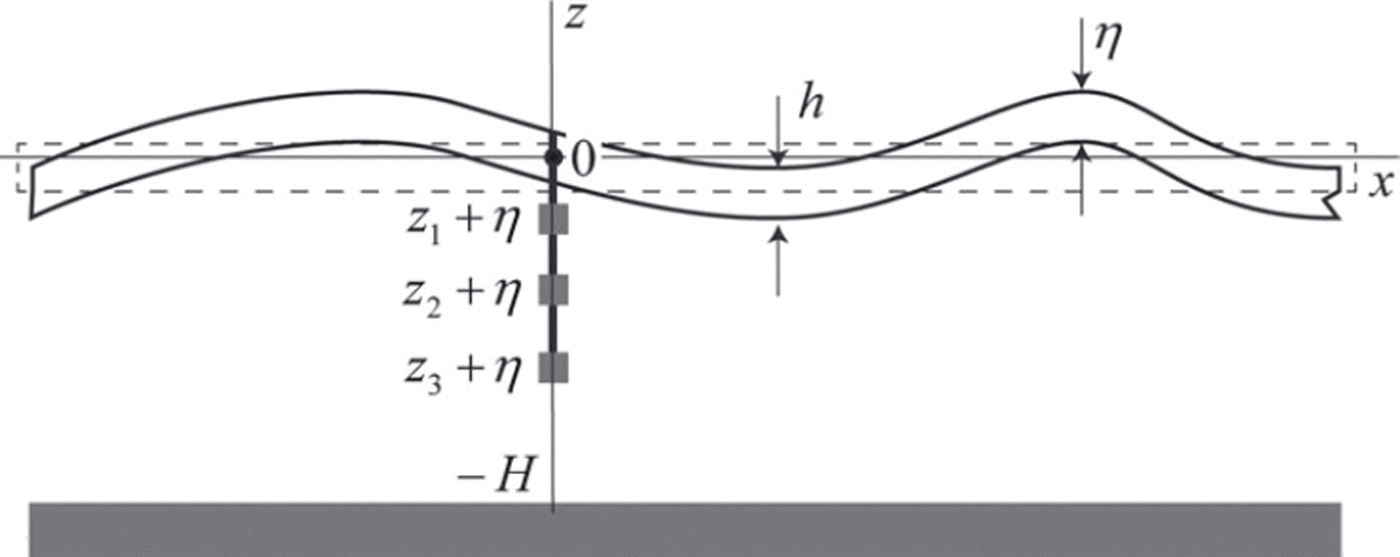
A water layer below the floating elastic ice sheet is considered (Fig. 1). Equations describing propagation of flexural-gravity waves in a floating ice sheet were first formulated by Reference GreenhillGreenhill (1886) and were subsequently used by many authors to investigate the interaction of surface waves with floating ice (e.g. Reference SquireSquire, 2007). Complex velocity potential, , describing a periodic surface wave of small amplitude in a water layer of depth H, is determined by

where x =( x,y) and z are horizontal and vertical coordinates, t is the time, and k = (k_x,k_y) and ω are wave vector and wave frequency, k = \k\. The velocity of a fluid particle is given by the gradient vector (∂Φ/∂x,∂Φ/∂y,∂Φ/∂z). Amplitudes of the velocity potential, 2 ₀, and the elevation of water-ice surface, 2 ₀, are coupled by the formula k ₀tanh [kH] = –iω_η0 following from the kinematic condition at the ice/water interface.

Fig. 1.

Water layer beneath an elastic ice sheet. Scheme of deployment of three pressure sensors mounted under the floating ice.

The frequency and wave vector satisfy the dispersion equation

where E and v are the Young’s modulus and Poisson’s ratio of the ice, h is the ice thickness, p_w is the water density and g is gravity acceleration. Dispersion equation (2) is derived from Bernoulli’s equation at the ice/water interface with assumptions that the ice thickness is much smaller than the water depth and the wavelength is much greater than the ice thickness. The influence of the ice draft on the wave properties is important when the first assumption is not satisfied (Reference Squire, Vaughan and BennettsSquire and others, 2009). The second assumption allows us to use the theory of thin elastic plates (Reference Landau and LifshitzLandau and Lifshitz, 1986) to describe bending deformations of floating ice.

Representative values of E and v are equal to

In natural conditions, Young’s modulus varies over the ice thickness. Reference Kerr and PalmerKerr and Palmer (1972) have shown that a modified flexural stiffness d may be introduced in this case, which allows use of a fully homogeneous plate theory with the effective elastic modulus E.

Water pressure measured at distance z from the moving ice/water interface consists of hydrostatic (p _gst) and dynamic (p _dyn) terms determined by the formulas

following from the Bernoulli equation. The dynamic part of the pressure becomes equal to zero when water motion is absent.

Substituting Eqn (1) into Eqn (4) and expressing ₀ by ₀ we find that the dynamic water pressure induced by the wave solution (1) is expressed by

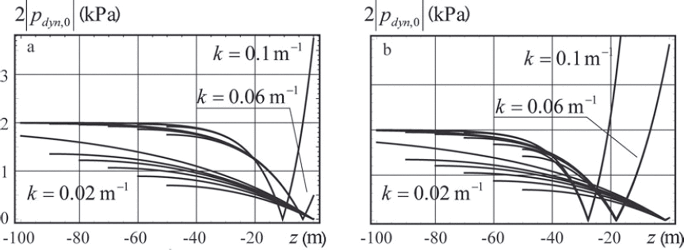
Figure 2 illustrates the dependence of vertical profiles of 2|p _dyn,0| from depth z. The ice thickness is h=1m in Figure 2a and h = 2m in Figure 2b. The graphs are constructed for three values of the wavenumber: k= 0.1 m–¹, k=0.06m–¹ and k=0.02m–¹. For each of these values, the graphs are constructed for the water depths 50, 60, 70, 80, 90 and 300 m. All graphs constructed with the same wavenumber begin from the same point, z= 0. They are very close to each other for relatively small depths, and their divergence increases with increasing depth. The divergence is stronger for smaller wavenumbers. The absolute value of the water pressure amplitude at the bottom increases with increasing water depth. The amplitude of the water pressure approaches 2p _wgη0 at great depths.

Fig. 2.

Profiles of absolute values of the water pressure amplitude over the vertical water column are constructed with ice thickness 1 m (a) and 2 m (b).

3. Estimate of Ice Stiffness from Pressure Characteristics of Flexural-Gravity Waves

It is assumed that three pressure sensors are mounted under the floating ice with a rope at distances z₁, z₂ and z ₃ from the imaginary water surface located at z=0 in the rest state (Fig. 1). The vertical positions of the sensors in the absolute frame of reference are z₁ + , ,z₂ + and z₃ + since the sensors move together with the ice when the ice is deformed by propagating waves. Each of the sensors records the water pressure at discrete moments in time. Frequencies of the waves with maximal energy can be calculated from spectral analysis.

Consider one of these frequencies, , and assume that the spectral amplitudes of the pressures recorded by the sensors at frequency ω are equal to p ₁,_dyn, p _2,dyn and p ₃,_dyn. The ratios of these amplitudes are written according to Eqn (5) as follows:

Wavenumber k and water depth H are calculated from Eqns (6) and (7) when 7₁₂, 7₁₃ and ω are known. The ice stiffness d is calculated afterwards from the dispersion equation (2).

It is assumed that ₁₂, ₁₃ and ω are determined from an experiment with certain accuracy and their random variations around actual values _12,0, _13,0 a n d ₀ are equal to ₁₂, ₁₃ and . Quantities mω = ω, m _γ12 = Δγ₁₂/γ_12,0 and m _γ13 = Δγ₁₃/γ_13,0 are the relative errors of the measurements of the wave frequency ω and the ratios 7₁₂ and 7₁₃. They influence errors in the calculation of the ice flexural stiffness and the water depth. Further, we analyse the dependence of the relative errors in the calculation of the flexural stiffness md = Δd/d₀ and the water depth mH = ΔH/H₀ from the relative errors m_u, m ₂ and m ₁₃. Numerical estimates are performed with m ₁₂ = m ₁₃ = m ₇ = ±0:05 where m _w is equal to -0.05, 0 and 0.05.

The explicit solution of Eqns (2), (6) and (7) is expressed by

when ω = ω ₀, 7₁₂ = 7_12,0, 7₁₃ = 7_13,0. Variations of k, Hand d are related to the variations of 7₁₂, 7₁₃ and ω according to

where all partial derivatives are calculated using Eqns (6) and (7) and dispersion equation (2). All derivatives in Eqns (9) and (10) are calculated in the point of the explicit solution.

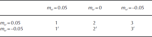
Figures 3 and 4 show relative errors md and m_H versus the wave frequency c^₀. It is assumed that the ice thickness is h=1 m and pressure sensors 2 and 3 are located at depths z ₂ = -10m and z ₃ =-15 m, with pressure sensor 1 located at depth z ₁=-2m (Fig. 3) and z ₁=-5m (Fig. 4). The water depth is given in the figure captions. Specifications of the curves shown in the figures are given in Table 1.

Fig. 3.

Relative errors of the flexural stiffness md and the water depth m_H versus the wave frequency ω ₀. Pressure sensors are deployed at depths z ₁ =-2m, z ₂ =-10m and z ₃ =-15 m.

Fig. 4.

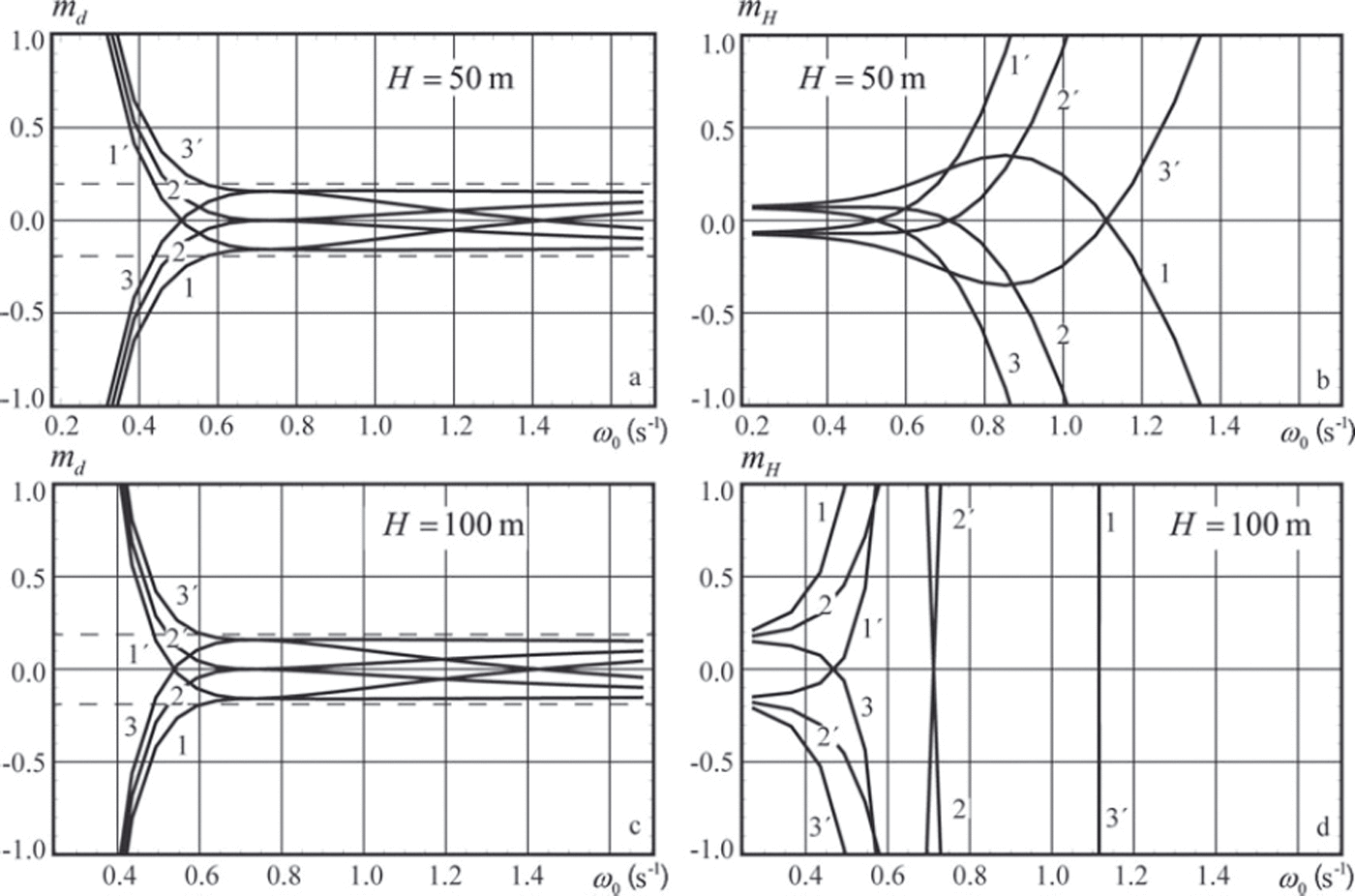
Same as Figure 3, but depths are z ₁ =–5m, z ₂ =–10m and z ₃ = –15 m.

Table 1.

Specification of curves shown in Figures 3–6

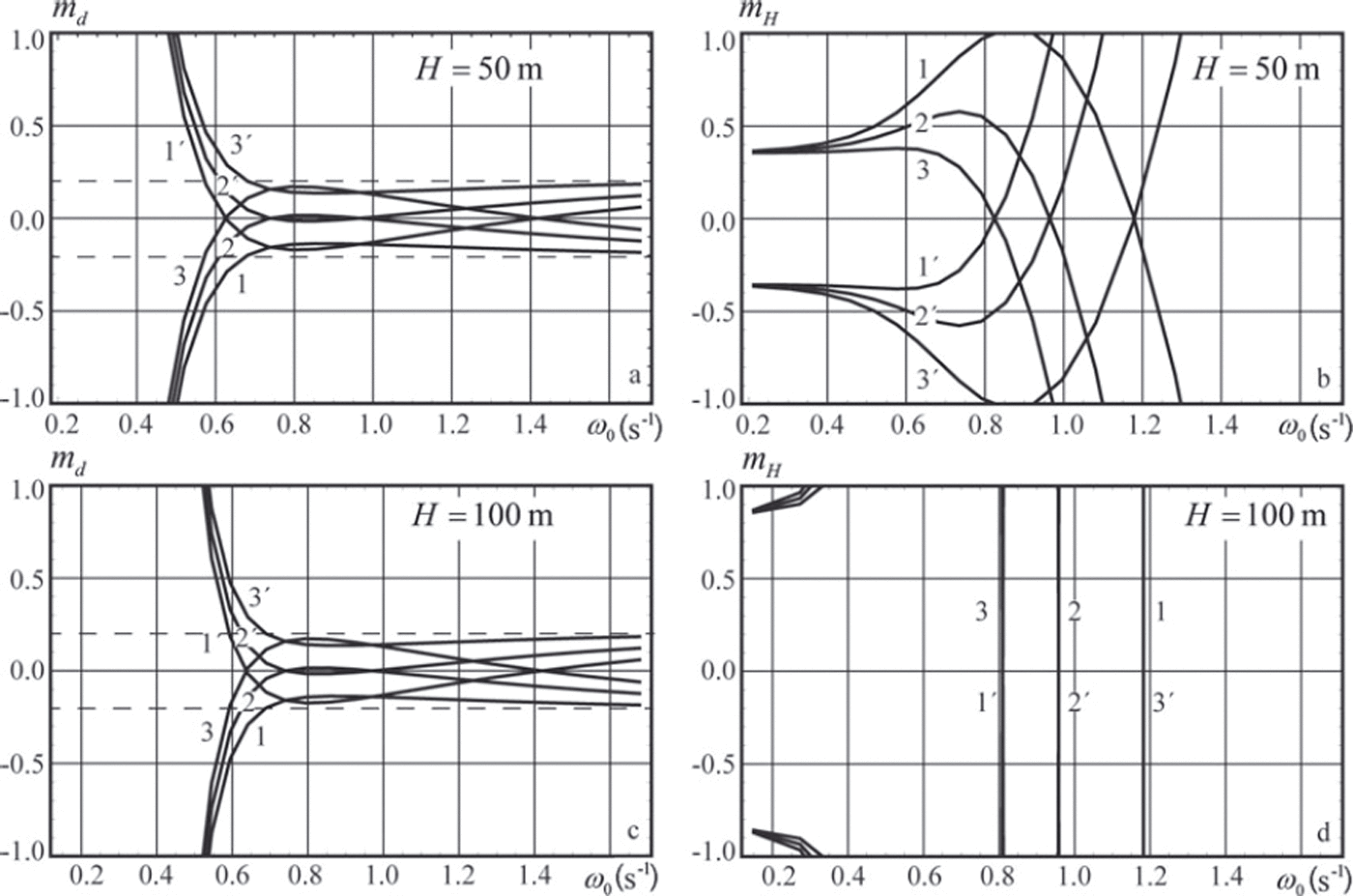
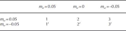
The relative error md does not exceed 2 0% when the wave frequency ω0 > 0.6s–¹ (wave period T0 = 2π/ω₀ < 10.5s) in Figure 3a and c, and when the wave frequency ω₀ > 0.7s-¹ (T ₀<9s) in Figure 4a and c. Thus the accuracy in the definition of flexural stiffness is higher when the distance between the ice bottom and sensor 1 is smaller. The relative error m_H is <10% when the wave frequency is <0.4s–¹ (T ₀> 1 5 . 7 s) in Figure 3b. Figure 3d shows that m_H is very high when the wave frequency is >0.3 s–¹. Thus the longwave part of the wave spectrum provides the most useful information for estimates of water depth, while the shortwave part provides the most useful information for estimates of flexural stiffness.

Equations (2) and (6) are used for calculation of the wavenumber and the flexural stiffness when the wave frequency ω₀, the ratio 7_12,0 and the water depth H₀ are known. In this case, variations of k and d are coupled with the variations of ₁₂, ₁₃ and by

where all partial derivatives are calculated taking into account Eqn (6) and dispersion equation (2) in the point of the explicit solution.

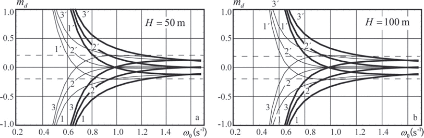
Results of the numerical simulations are shown in Figures 5 and 6. Specifications of the curves shown in the figures are given in Table 1. The ice thickness is h=1 m. Vertical coordinates z₁ and z ₂ of the pressure sensors and the water depth are shown in the figure captions. Variations of the water depth within mH = ±0.1 have very little influence on the shape of the curves shown in Figures 5 and 6. Therefore the dependence of the relative error md on m_H is not discussed.

Fig. 5.

Relative errors of the flexural stiffness m_d versus the wave frequency ω₀. Pressure sensors are deployed at depths z ₁ = –10 m, z ₂ = –15 m (thick lines) and z ₁ = –5 m, z ₂ = –10 m (thin lines).

Fig. 6.

Same as Figure 5, but depths are z ₁ =–2m, z ₂ =–15m (thick lines) and z ₁ = 0 , z ₂= –15m (thin lines).

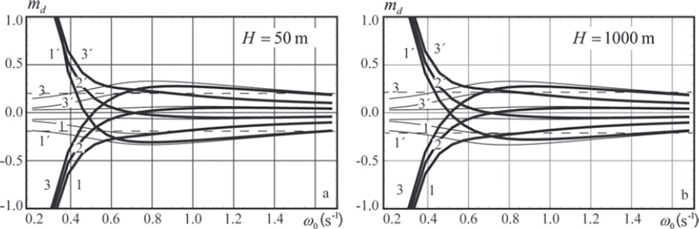
Figure 5 shows that the relative error md does not exceed 20% when the wave frequency ω₀ > 0.9s–¹ and the sensors are located at depths z ₁=-5m and z ₂=-10m. For the sensors located at depths z₁ = -10m , z ₂=-15 m the relative errors are <20% when the wave frequency ω₀ > 1.2s_¹. Figure 6 shows that md does not exceed 30% when pressure sensor 1 is located just below the bottom of the ice and Ω ₀ > 0 . 2 s ^{- 1} (T ₀<31.4s). Downward displacement of the pressure sensor at 2 m depth below the ice shrinks the range of wave frequencies providing 30% accuracy of the ice stiffness calculation to ω₀ > 0.6s^-1 . Figures 5 and 6 demonstrate that the water depth H₀ has little influence on the dependence of m_d on ω₀.

4. Estimates of Effective Elastic Modulus of Sea Ice using Data from Field Measurements

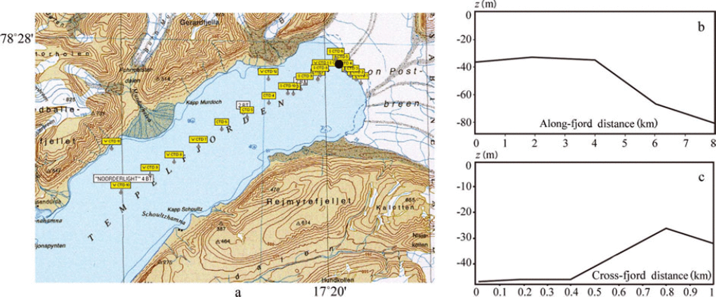
Fieldwork was performed in Tempelfjorden near the glacier front in 2011 and 2012 (Fig. 7a). The map of Templefjorden is taken from the Svalbard map of the Norwegian Polar Institute (www.npolar.no). The glacier front was mapped in 1990 using aerial photographs. Two profiles of the sea bottom along and across the fjord near the glacier front are shown in Figure 7b and c. The glacier front of ∼3 km width is formed by the outflow glaciers Tunabreen and Von Postbreen. Measurements with a Leica Total Station confirm that the height of the glacier wall reached 37 m above water level near the fieldwork site. The sea-ice thickness near the glacier front was ∼1 m in both 2011 and 2012. Snow thickness did not exceed 15 cm. Temperature profiles through the ice were almost linear, with the ice just under the snow being about -5°C and at the bottom of the ice about -1.9°C. Mean salinity of the ice was 5-6ppt (Reference Marchenko, Morozov and MuzylevMarchenko and others, 2012).

Fig. 7.

(a) Map of Tempelfjorden. Locations of sea depth measurements are marked by yellow squares and the location of the water pressure measurements by a black dot. (b, c) Sea bottom profiles along the fjord (b) and across the fjord (c).

Although the glaciers have been stable since 2005, significant buckling deformations and folds were observed in the sea ice near the front of Tunabreen in February 2011 (Fig. 8a). In 2012 the winter was warmer and the glacier front was less stable. Ice blocks were observed to fall on the surface of the sea ice near the glacier in April. Surface waves excited by these events broke the sea ice into polygonal blocks near the glacier (Fig. 8b). It should also be mentioned that the surface of the sea ice near the glacier front was flatter in 2012 than in 2011. This is probably because less of Tempelfjorden was covered by sea ice in 2012 than in 2011.

Fig. 8.

Sea ice near the glacier front in February 2011 (a) and April 2012 (b).

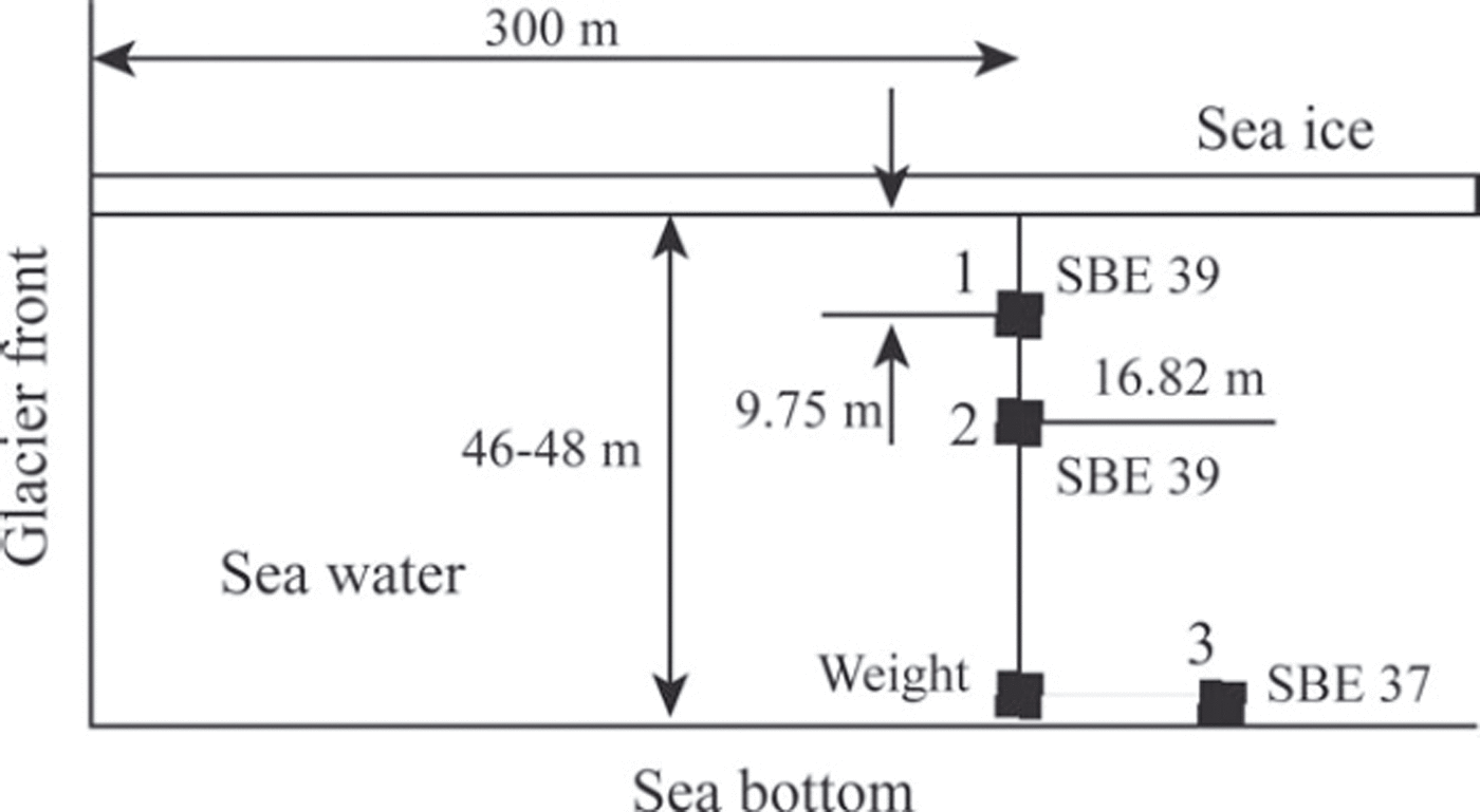
The location of the field measurements in February 2011 is shown with a black dot in Figure 7a. The ice thickness measured in the borehole was 94 cm. Two SBE 39 temperature and pressure recorders (sensors 1 and 2) were deployed through the borehole to depths z₁=-9.75m and z₂ = -16.82 m at a distance of ∼300 m from the Tunabreen front. They recorded the pressure and temperature with a sampling interval of 1 s. The pressure sensor in the SBE 39 recorders is designed for water pressure measurements up to 20 m depth and has initial accuracy of 2 cm and a resolution of 0.4 mm. An SBE 37 instrument (sensor 3) was deployed at the bottom of the water column at the same point, with a sampling interval of 6s. The scheme of the deployment is shown in Figure 9. The weight was used to keep sensor 3 at the bottom when the water level changed due to the tide. Water-pressure records at the bottom show dominant semidiurnal variations of water depth between 46 m and 48 m (Fig. 10a). The time in Figure 10a is given in hours from the beginning of the field measurements.

Fig. 9.

Scheme of the deployment of pressure sensors 1–3 near the glacier front.

Fig. 10.

Records from pressure sensors 3 (a, b), 1 (c) and 2 (d).

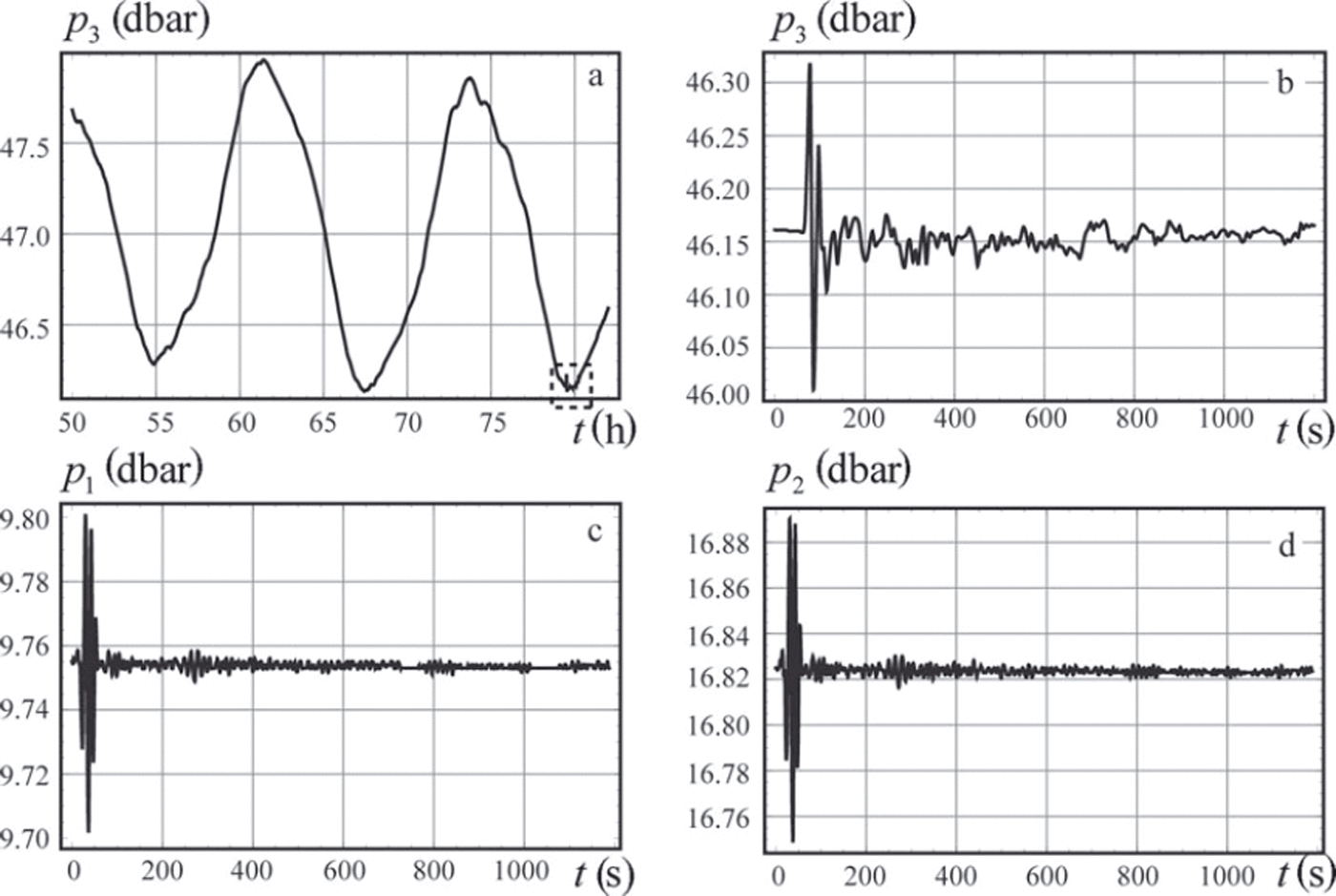
At approximately 07:40 on 17 February the instruments recorded a tsunami wave event, shown within the dashed rectangle in Figure 10a. Records from the pressure sensors are shown in Figure 10b-d where the time is indicated in seconds from the beginning of the tsunami event. Spectral analysis of the leading wave pulse, which displaced the ice vertically by ∼30cm, was performed by Reference Marchenko, Morozov and MuzylevMarchenko and others (2012). In the present paper, we analyse properties of the wave tail to estimate the ice flexural stiffness. Since the ice thickness was measured (h = 94cm) and the Poisson’s ratio is very stable for ice (v = 0.31-0.34), the estimates provide information on the effective elastic modulus, E, of sea ice in bending deformations. Records from sensor 3 deployed at the bottom show a water depth of H₀ = 46.15 m at the moment of the tsunami event.

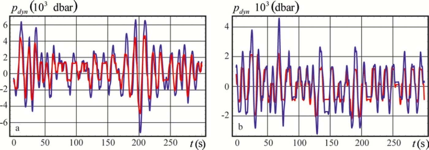
Two ccntervals of the wave tail record were used for the calculation of the effective elastic modulus. The wave tail intervals are shown in Figure 10c and d by t ∈ (70 s, 370 s) and t ∈ (370 s, 670 s) respectively. The dynamic water pressure is shown in Figure 11a and b versus the time for the first and second intervals respectively. The time is accounted from the beginning of each interval in Figure 11a and b. The red and the blue lines are related to the records of sensors 1 and 2. Figure 11 shows about four to five oscillations per 50 s and significant modulations of their amplitude over 2-3 min. The wave period is roughly estimated to be 10-12.5 s, and the estimated wave frequency is 0.5-0.63 s–¹. Using the dispersion equation (2) with water depth H₀ = 46.15 m and representative values (Eqn (3)) we found that the wavenumber varies between 0.026m–¹ and 0.045 m–¹. Theoretical curves in Figure 2a and experimental records in Figure 11 both demonstrate that the amplitude of the dynamic pressure at the depth z₁ = -9.75 m is lower than the dynamic pressure amplitude at the depth z₂ =-16.82 m.

Fig. 11.

Dynamic water pressure p _dyn versus the time t recorded in two consecutive time intervals at depths z ₁ = –9.75 m (red lines) and z ₂ = –16.82 m (blue lines).

The Fourier transform of the dynamic pressure records is calculated using

Data processing for each list of the dynamic pressure data was done in the following steps. Raw data arranged as a list of the time and pressure values with 1 s temporal resolution were interpolated using the procedure Interpolation in Mathematica 8 with default setting InterpolationOrder → 3. Then a new list with finer temporal resolution of 0.1 s was formed for the numerical calculation of the Fourier integral (Eqn (13)). The finer resolution was used to smooth the integrand expression in Eqn (13) according to the assumption about continuity of the pressure dependence on the time. The integral was calculated as a sum of the integrand expressions in the points t = t_j multiplied by dt = 0.1 s for frequency values in the range w ε (0,3)s–¹ with a resolution of 0.001 s–¹. Absolute values |p _F| of the Fourier integrals shown in Figure 12a and b versus the frequency are smoothed using the MovingAverage procedure over 60 points in Mathematica 8. The red and the blue curves correspond to the pressure records at depths z₁=-9.75m and z ₂=-16.82m. Spectral peaks of the dynamic pressure are located in the range ω ε (0.2,0.8)s-¹. The main spectral maximum is in the range ω (0.35,0.5)s^-1.

Fig. 12.

Absolute value | pF| of the Fourier transform of the dynamic pressure (a, b) and calculated effective elastic modulus E (c, d) versus the wave frequency in two consecutive fragments of the wave tail.

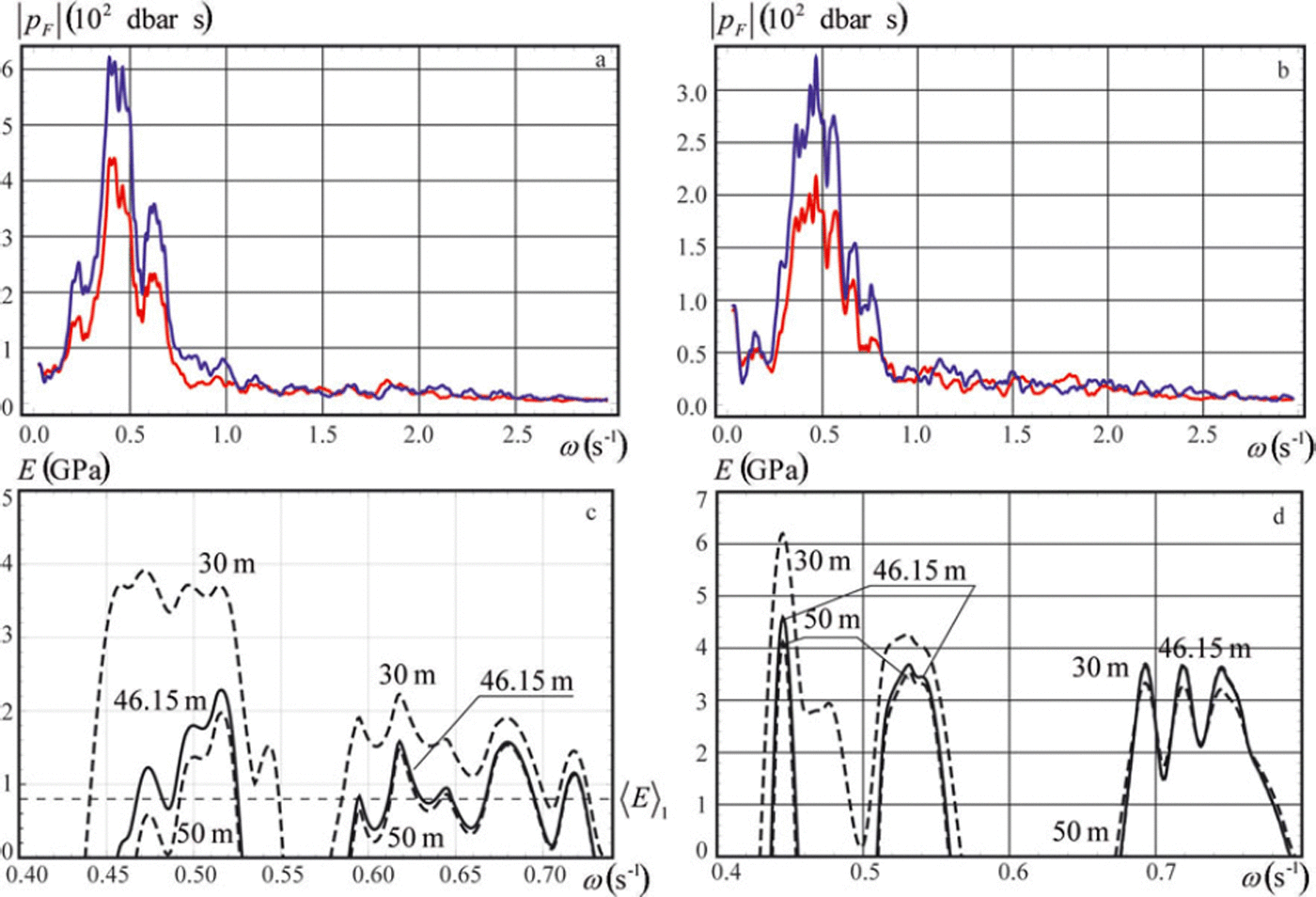
In the next step, the wavenumbers were calculated numerically using Eqn (6) with the procedure FindRoot in Mathematica 8 for each value of the wave frequency in the range ω (0.4,0.8)s^-1 with a resolution of 0.001 s–¹. Values of the effective elastic modulus calculated from the dispersion equation (2) are shown in Figure 12c and d by continuous lines when H₀ = 46.15 m and by dashed lines when H ₀ = 30m and H ₀ = 50 m. The ice thickness and Poisson’s ratio are h = 94 cm and v = 0.33. Negative values of E are not shown in the figures. Both figures demonstrate little dependence of E on the water depth variations in the frequency range ω > 0.6s^-1.

The quality of the data performed in Figure 11a and b can be estimated as a ratio, R, of the resolution of the pressure sensor in recorder SBE 39 (r=4mm) to the mean values of double amplitude of the dynamic pressure oscillations. The mean amplitudes are estimated as standard deviations σ _a , _i and σb _, i of the pressure data shown in Figure 11a and b, where i=1 for the measurements at z=z ₁, and i=2 for the measurements at z=z₂. We found σ _{a , 1} =1:65 mm, _{a, 2} = 2:43 mm, j _{b , 1} = 0:96mm and _{b ,}2 = 1:37mm. Ratios R are equal to R_{a , 1} = 0:12, R_a,2 = 0:08, R_{b , 1} = 0:21 and Rb_,2 = 0:15. Since R_a, ₁ /Rb,₁ = 0:57 and R_a,2/Rb,₂ = 0:53 the quality of the data shown in Figure 11a is better than that shown in Figure 11b by a factor of almost two. Therefore the best estimate of the effective elastic modulus is given by the high-frequency part of the wave signal shown in Figure 12a with frequencies in the range ω <E (0:59,0:76) s^-1. The maximal value of the effective elastic modulus 1.6GPa at the frequency ω = 0:62s^-1 in Figure 12c is related to the spectral peak in Figure 12a at the same frequency. The mean value of the effective elastic modulus is 〈E〈₁ = 0:77GPa.

The brine volume of sea ice in the range of the fieldwork was calculated with the formula v = (49:185/| T| + 0:532) (Reference Frankenstein and GarnerFrankenstein and Garner, 1967), where T is the ice temperature and σ is the ice salinity. At the ice surface T=-5°C, σ=5ppt and the brine volume is equal to 50.8ppt, and at the ice bottom T=-1.9°C, σ = 6ppt and the brine volume is equal to 155.4ppt. The mean value of the brine volume over the ice thickness is 103.1ppt. The effective elastic modulus calculated with the formula of Vaudrey (1977), is equal to 0.88 GPa when v= 103.1ppt. This value is close to (E)₁ = 0:77GPa.

5. Conclusions

A new method for calculation of the ice flexural stiffness has been described and analysed. It is based on the analysis of water pressure records at two or three locations below the ice bottom when flexural-gravity waves propagate below the ice. The analysis of the relative errors in the definition of the ice flexural stiffness shows that these errors decrease with increasing wave frequency. The relative errors are also smaller when one of the pressure sensors is deployed immediately below the ice while the other sensors are deployed at about 10-15 m depth. The sampling frequency of the pressure sensors should be not less than 1 Hz.

The method was tested using data from field measurements in Tempelfjorden. Flexural-gravity waves were excited by an icefall at the front of the outflow glacier Tunabreen in February 2011. The water pressure was recorded by two sensors deployed at depths z₁ =-9.75 m and z₂ =-16.82 m below the ice. The water depth was measured with a pressure sensor deployed at the sea bottom. The ice thickness was measured by drilling. Temperature and salinity measurements showed mean brine volume in the ice was ∼100ppt.

Several spectral peaks were found in the frequency range ω ε (0:2,0:8)s^–1. The error analysis shows that the wave signal is an insufficient predictor for calculating the ice flexural stiffness in the frequency range below 0.6 s–¹. Therefore the wave spectrum in the higher-frequency range was used for calculation of the ice flexural stiffness and the effective elastic modulus. The calculated mean value of the effective elastic modulus (E)₁ = 0:77GPa is close to the value of the effective elastic modulus 0.88 GPa calculated with the formula of Reference VaudreyVaudrey (1977).