1 Introduction
Droplet dynamics in microfluidic Hele-Shaw cells has garnered much interest in the last decade due to the many applications to which it is relevant. Notably, they have much promise for large-scale automation of chemistry and biology microfluidic-based systems (Garstecki et al. Reference Garstecki, Gitlin, Diluzio, Whitesides, Kumacheva and Stone2004; Link et al. Reference Link, Anna, Weitz and Stone2004; Stone, Stroock & Ajdari Reference Stone, Stroock and Ajdari2004; Joanicot & Ajdari Reference Joanicot and Ajdari2005; Squires & Quake Reference Squires and Quake2005; Pompano et al. Reference Pompano, Liu, Du and Ismagilov2011). No less important, these same microfluidic systems also provide a platform to research fundamental science such as the effect of capillary number, the flow rate ratio and more (Christopher et al. Reference Christopher, Noharuddin, Taylor and Anna2008; Belloul et al. Reference Belloul, Engl, Colin, Panizza and Ajdari2009).
A decade ago, Beatus, Tlusty & Bar-Ziv (Reference Beatus, Tlusty and Bar-Ziv2006) showed that the dispersion relation of an infinite translating lattice of droplets in a Hele-Shaw microchannel was analogous to that of phonons in a static solid-state crystal (Kittel Reference Kittel1986). This dispersion relation was derived under the assumption that the flow around each droplet was like the classical potential flow around a cylinder and the interactions between droplets were dipolar. It is well known in fluid mechanics that the superposition of uniform and single dipole flows gives the classical solution of a flow around a cylinder, which satisfies a no-flux condition at the surface (Landau & Lifshitz Reference Landau and Lifshitz1959; Currie Reference Currie1974). By adding additional dipolar interactions, the no-flux condition at each droplet surface is violated. Yet the resulting dipole model described experiments remarkably well (Beatus et al. Reference Beatus, Tlusty and Bar-Ziv2006), even at small spacing where it is expected to fail. Since then the dipole model has become the hallmark model used for the investigation of interactions for systems of two or more droplets (Champagne et al. Reference Champagne, Vasseur, Montourcy and Bartolo2010; Champagne, Lauga & Bartolo Reference Champagne, Lauga and Bartolo2011; Liu, Goree & Feng Reference Liu, Goree and Feng2012; Uspal & Doyle Reference Uspal and Doyle2012a ,Reference Uspal and Doyle b ; Desreumaux et al. Reference Desreumaux, Caussin, Jeanneret, Lauga and Bartolo2013; Shani et al. Reference Shani, Beatus, Bar-Ziv and Tlusty2014), including a mean-field approach, as well as the effects of confinement (Beatus, Bar-Ziv & Tlusty Reference Beatus, Bar-Ziv and Tlusty2007) and the formation of Burgers shock waves (Beatus, Tlusty & Bar-Ziv Reference Beatus, Tlusty and Bar-Ziv2009) in a microfluidics channel.
Later, Beatus, Bar-Ziv & Tlusty (Reference Beatus, Bar-Ziv and Tlusty2012) justified that using an infinite amount of reflections would result in a de facto no-flux boundary condition (BC). However, their argument was limited to two droplets (Beatus et al. Reference Beatus, Bar-Ziv and Tlusty2012): ‘Unfortunately, generalizing the method of reflections for three droplets or more is too cumbersome, since it involves enumerating the reflections created by more than two surfaces.’ Owing to its inherent complexity, this two-droplet infinite-sum reflection potential was never tested for the dynamics of two droplets. While it is not surprising that the dipole model works at very large spacing, one should ask: Why does the model work at intermediate spacing when one does not expect the interactions to be purely dipolar?
In contrast to these many-body works, Sarig, Starosvetsky & Gat (Reference Sarig, Starosvetsky and Gat2016) recently studied the dynamics of a two-droplet system in a Hele-Shaw channel. There, they solved for the pressure field for two arbitrarily sized and arbitrarily spaced droplets. Using bipolar-cylindrical coordinates, they derived an analytical solution, for the pressure field and forces on the droplets, in terms of infinite Fourier series, that satisfies the no-flux BC. Unfortunately, while their solution is exact, its complicated form does not allow for any additional straightforward analysis, including derivation of zeroth- and first-order dynamical equations. Upon simple inspection, their solution does not appear to reduce to the dipole solution, as is expected at large spacing. In this work, we will show that indeed it does, and we derive a new approximation for small spacing.
This work will be divided into two:
 $N=2$
droplets (§§ 2 and 4) and
 $N>2$
droplets (§ 5). In § 2 we present a short summary of the work by Sarig et al. (Reference Sarig, Starosvetsky and Gat2016), which introduces the Fourier series and the forces. In § 3 we derive approximations for the Fourier series terms for large and small spacing. We then analyse the interplay of the various forces and rationalize why the dipole model appears to be successful even at small spacing. In § 4 we derive the zeroth- and first-order equations governing the two-droplet dynamics, which includes a new term in the perturbation equation. In § 5 we generalize our approach, for large spacing, from
 $N=2$
to any
 $N>2$
system and analyse these
 $N>2$
systems. Concluding remarks are given in § 6.
2 Two-droplet problem definition
In general, in Hele-Shaw channels, the spacing separating the two surfaces,
 $\tilde{h}$
(where tilde marks dimensional units), is much smaller than all other length scales in the system. If inertia is negligible, the in-plane velocities are related to the pressure via
 $\tilde{\boldsymbol{u}}=-(\tilde{h}^{2}/12\tilde{\unicode[STIX]{x1D707}}_{F})\tilde{\unicode[STIX]{x1D735}}\tilde{p}$
and the in-plane pressure is determined by
 $\tilde{\unicode[STIX]{x1D6FB}}^{2}\tilde{p}=0$
, where
 $\tilde{\unicode[STIX]{x1D707}}_{F}$
is the viscosity of the background fluid. To simplify to
 $\boldsymbol{u}=-\unicode[STIX]{x1D735}p$
, the velocity is normalized by a characteristic velocity
 $\tilde{U}$
, and the in-plane length scales are normalized by an in-plane characteristic length (discussed later),
 $\tilde{L}$
, such that the pressure scales as
 $12\tilde{\unicode[STIX]{x1D707}}_{F}\tilde{U} \tilde{L}\tilde{h}^{-2}$
.
That low-Reynolds-number flows can be described by a potential formulation has been leveraged to simplify the mathematical analysis of otherwise complicated problems. Perhaps the most notable is the Saffman–Taylor fingering instability whereby a less viscous fluid is injected into a more viscous fluid and the interface is unstable to transverse perturbations, leading to the formation of large fingers (Saffman & Taylor Reference Saffman and Taylor1958). The case of small droplets was also analysed, and it was shown that surface tension ensures that the droplets are circular and stable (Taylor & Saffman Reference Taylor and Saffman1959; Tanveer Reference Tanveer1986). However, larger droplets can also have non-circular geometries (Tanveer Reference Tanveer1986; Green, Lustri & McCue Reference Green, Lustri and McCue2017) (see the discussion regarding the extraordinary branch in Tanveer (Reference Tanveer1986)). In this work we shall consider only circular droplets, which are of interest to numerous applications (Pompano et al. Reference Pompano, Liu, Du and Ismagilov2011), and were considered in Sarig et al. (Reference Sarig, Starosvetsky and Gat2016) whose results we are extending.
One final comment is in order on the relation between Hele-Shaw flows and potential flows. In this work, we will be using the results derived in Sarig et al. (Reference Sarig, Starosvetsky and Gat2016), who solved the Laplace equation in bipolar-cylindrical coordinates for the flow field around two circular cylinders under the assumption of a Hele-Shaw cell. However, a similar solution has already been derived in potential flows without the assumption of bipolar coordinates. The Villat formula gives a closed-form solution to the flow field around two cylinders in terms of an integral (Crowdy, Surana & Yick Reference Crowdy, Surana and Yick2007). Thus, the large- and small-spacing approximations derived in this work are perhaps relevant and their concepts can be extended in the context of the Villat formula.
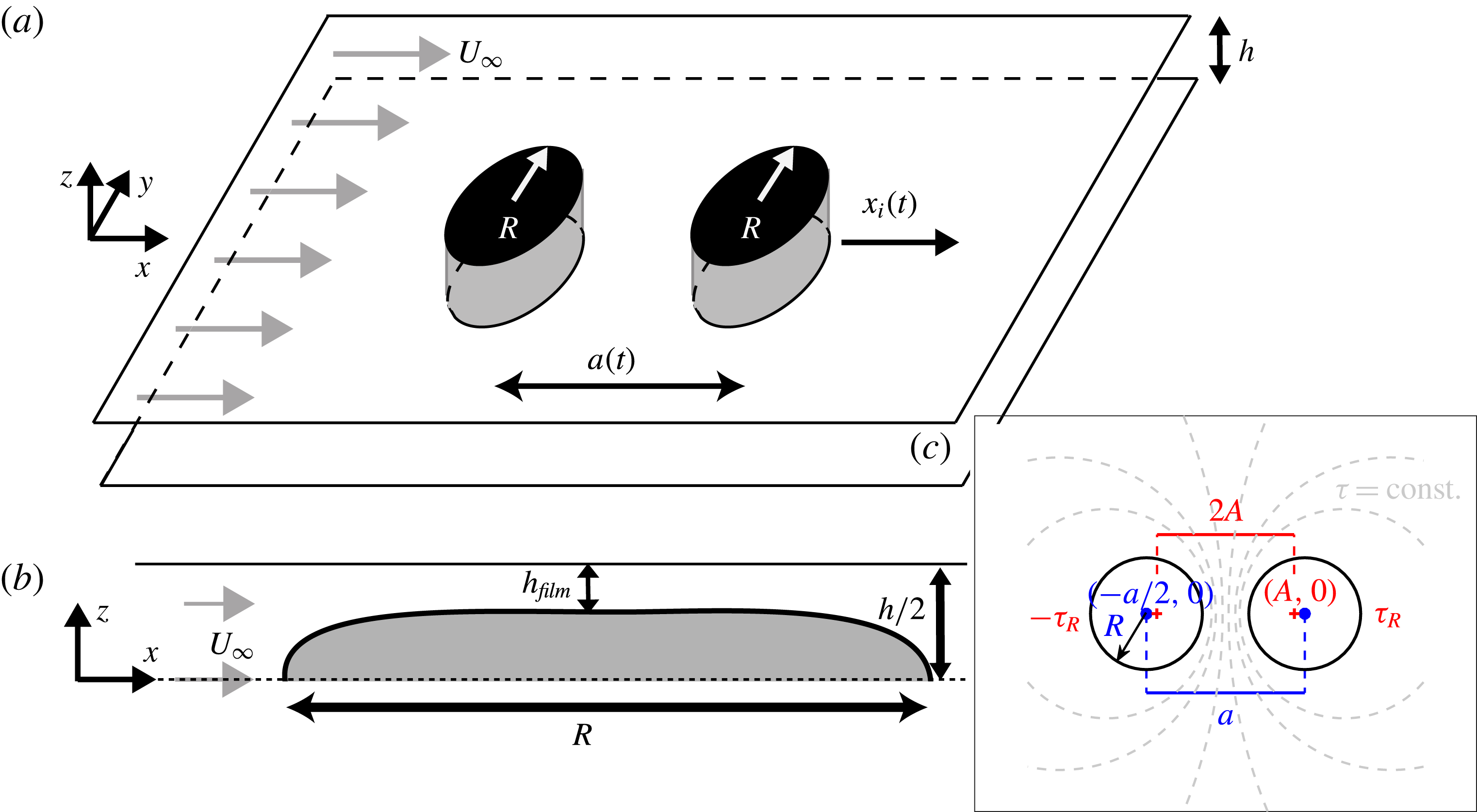
Our system comprises two identical droplets, of radius
 $R$
and viscosity
 $\tilde{\unicode[STIX]{x1D707}}_{d}$
, confined in a Hele-Shaw cell of height
 $h$
(see figure 1
a for a schematic). The background fluid has a viscosity
 $\tilde{\unicode[STIX]{x1D707}}_{F}$
and far from the droplets it is assumed that the fluid moves with a uniform flow velocity of
 $U_{\infty }$
in the
 $\hat{\boldsymbol{x}}$
direction, which is aligned with the axis connecting the droplets’ centres. The droplet’s centres are separated by a spacing distance
 $a(t)$
.
(a) Schematic description of the two-droplet set-up. The droplets are separated by a distance
 $a(t)$
, confined between two plates separated by a distance
 $h$
in the
 $\hat{z}$
direction, and have a radius
 $R$
. The streaming velocity of the fluid is
 $U_{\infty }$
. The coordinate
 $\hat{\boldsymbol{x}}$
is aligned along the axis line connecting the centres of the droplets. (b) Side view of a droplet in the channel. There is a thin film of fluid between the droplet and substrate with thickness
 $h_{film}$
. (c) Top view of the droplets. The bipolar parameters
 $A,\unicode[STIX]{x1D70F}_{R}$
(red markings) are related to
 $a,R$
(blue markings).
Sarig et al. (Reference Sarig, Starosvetsky and Gat2016) solved the Laplace equation, for the pressure, while satisfying the no-flux condition. Rather than treating the force on the droplet to be point-like, as the dipole model does, they integrated the pressure around each of the circular droplets and calculated the applied force. Their solution allowed for two-dimensional (2D) streaming flows (lateral and perpendicular flows). In this work we focus on one-dimensional (1D) lateral flows with identical droplets, as this corresponds to realistic experimental and numerical set-ups (Beatus et al. Reference Beatus, Tlusty and Bar-Ziv2006, Reference Beatus, Bar-Ziv and Tlusty2007; Champagne et al. Reference Champagne, Vasseur, Montourcy and Bartolo2010; Liu et al. Reference Liu, Goree and Feng2012). However, our approximations can also be extended to solve 2D problems.
When the flow is aligned with the axis between the two centres of mass (
 $\hat{\boldsymbol{x}}$
direction), the non-dimensional force acting on the
 $i\text{th}$
droplet is (Sarig et al.
Reference Sarig, Starosvetsky and Gat2016)
 $$\begin{eqnarray}\displaystyle & \displaystyle F_{i}=F_{s}+F_{pressure}+F_{friction}+F_{int}=0, & \displaystyle\end{eqnarray}$$
 $$\begin{eqnarray}\displaystyle & \displaystyle F_{s}=4\unicode[STIX]{x03C0}A^{2}(U_{\infty }-{\dot{x}}_{i})Q_{s}, & \displaystyle\end{eqnarray}$$
 $$\begin{eqnarray}\displaystyle & \displaystyle F_{int}=4\unicode[STIX]{x03C0}A^{2}({\dot{x}}_{l}-U_{\infty })Q_{int}, & \displaystyle\end{eqnarray}$$
 $$\begin{eqnarray}\displaystyle & \displaystyle F_{pressure}=\unicode[STIX]{x03C0}R^{2}U_{\infty }, & \displaystyle\end{eqnarray}$$
 $$\begin{eqnarray}\displaystyle \displaystyle Q_{s}=\mathop{\sum }_{n=1}^{\infty }n\text{e}^{-2n\unicode[STIX]{x1D70F}_{R}}\,\text{coth}(2n\unicode[STIX]{x1D70F}_{R}),\quad Q_{int}=\mathop{\sum }_{n=1}^{\infty }n\text{e}^{-2n\unicode[STIX]{x1D70F}_{R}}\,\text{csch}(2n\unicode[STIX]{x1D70F}_{R}), & & \displaystyle\end{eqnarray}$$
where
 $i\neq l$
and
 ${\dot{x}}_{i}$
is the velocity of the
 $i\text{th}$
droplet. Following Sarig et al. (Reference Sarig, Starosvetsky and Gat2016), forces are normalized by
 $12\tilde{\unicode[STIX]{x1D707}}_{F}\tilde{U} \tilde{L}^{2}\tilde{h}^{-1}$
, where it is now obvious that
 $\tilde{L}$
can be either
 $\tilde{R}$
or
 $\tilde{a}$
, and
 $\tilde{L}\gg \tilde{h}$
. To avoid ambiguities when the spacing is infinite,
 $\tilde{L}=\tilde{R}$
is the preferred scaling. The bipolar cylindrical parameters
 $A$
and
 $\unicode[STIX]{x1D70F}_{R}$
will be discussed below. The droplet displacements can be written in the following manner:
 $$\begin{eqnarray}x_{i}(t)=x_{i}(t=0)+U_{d}t+\unicode[STIX]{x1D6FF}x_{i}(t).\end{eqnarray}$$
The third term is a perturbation term that describes small displacements about the leading-order translation term. It is assumed that the droplet velocities are identical. This need not be the case for non-symmetric droplets, as discussed in appendix A. The droplet spacing is
 $$\begin{eqnarray}a=a(t)=x_{i}(t)-x_{l}(t)=a_{0}+\unicode[STIX]{x1D6FF}x_{i}-\unicode[STIX]{x1D6FF}x_{l}=a_{0}+\unicode[STIX]{x0394}\unicode[STIX]{x1D6FF}x,\end{eqnarray}$$
where
 $a_{0}$
is the spacing at
 $t=0$
. The bipolar cylindrical parameters
 $A$
and
 $\unicode[STIX]{x1D70F}_{R}$
are related to
 $a$
and
 $R$
through the following relations (figure 1
c) (Sarig et al.
Reference Sarig, Starosvetsky and Gat2016):
 $$\begin{eqnarray}A=\frac{\sqrt{a^{2}-4R^{2}}}{2}\approx \left\{\begin{array}{@{}lc@{}}a/2, & a/R\gg 1\text{ or }\unicode[STIX]{x1D70F}_{R}\gg 1,\\ \sqrt{4\unicode[STIX]{x0394}\unicode[STIX]{x1D6FF}xR}, & A/R\ll 1\text{ or }\unicode[STIX]{x1D70F}_{R}\ll 1,\end{array}\right.\end{eqnarray}$$
 $$\begin{eqnarray}\displaystyle \unicode[STIX]{x1D70F}_{R}=\sinh ^{-1}\left(\frac{A}{R}\right)\approx \left\{\begin{array}{@{}lc@{}}\text{log}(a/R), & a/R\gg 1\text{ or }\unicode[STIX]{x1D70F}_{R}\gg 1,\\ A/R, & A/R\ll 1\text{ or }\unicode[STIX]{x1D70F}_{R}\ll 1.\end{array}\right. & & \displaystyle\end{eqnarray}$$
The expressions for
 $A$
and
 $\unicode[STIX]{x1D70F}_{R}$
are approximated for large spacing,
 $\unicode[STIX]{x1D70F}_{R}\gg 1$
, and small spacing,
 $\unicode[STIX]{x1D70F}_{R}\ll 1$
. In this paper, the notation
 $a/R$
and
 $A/R$
appears often. While similar, these are not to be taken as the same. The notation
 $a/R\gg 1$
implies that the droplets are almost isolated, while the notation
 $A/R\ll 1$
implies that the droplets are almost touching such that
 $a_{min}=2R$
(or
 $a/R\approx 2+\unicode[STIX]{x0394}\unicode[STIX]{x1D6FF}x/R$
). We note there is a difference in our notation of
 $\unicode[STIX]{x1D70F}_{R}$
versus that of Sarig et al. (Reference Sarig, Starosvetsky and Gat2016). In their work,
 $\unicode[STIX]{x1D70F}_{1,2}=\pm \unicode[STIX]{x1D70F}_{R}$
takes both positive and negative values (figure 1
c). However, the Fourier coefficients (2.5) depend only on
 $\left|\unicode[STIX]{x1D70F}_{R}\right|$
. For brevity, we refer only to the absolute value (see appendix A and Sarig et al. (Reference Sarig, Starosvetsky and Gat2016) for more details).
There are numerous forces that contribute to the governing equation (2.1). For the sake of clarity and brevity, from this point we distinguish only between the interaction term (2.3) and the direct term, which is the sum of all other terms
 $$\begin{eqnarray}F_{direct}=F_{s}+F_{pressure}+F_{friction}.\end{eqnarray}$$
The nomenclature direct and int for interaction will become more apparent in the next sections, where we will show that in the case of large spacing the direct force is independent of the spacing
 $a_{0}$
whereas the interaction term is
 $a_{0}$
-dependent. The interaction term is the drag contribution due to the fact that there are two droplets. The pressure term accounts for a force due a pressure gradient in the channel and is reminiscent of a buoyant-like force.
We are finally left with modelling the frictional force. Beatus et al. (Reference Beatus, Tlusty and Bar-Ziv2006, Reference Beatus, Bar-Ziv and Tlusty2007, Reference Beatus, Tlusty and Bar-Ziv2009, Reference Beatus, Bar-Ziv and Tlusty2012) modelled their friction force based on an energy argument where their friction coefficient,
 $\unicode[STIX]{x1D707}_{dipole}$
(not to be confused with the viscosity), had to be deduced for each experiment separately as the geometry and fluid properties were varied. In contrast, Sarig et al. (Reference Sarig, Starosvetsky and Gat2016) suggested that the dimensional friction force was
 $\tilde{F}_{friction}=12\unicode[STIX]{x03C0}\tilde{R}^{2}\tilde{U} _{d}\tilde{h}^{-1}(2\tilde{\unicode[STIX]{x1D707}}_{d}+\tilde{\unicode[STIX]{x1D707}}_{F}-2\tilde{\unicode[STIX]{x1D707}}_{F}/\unicode[STIX]{x1D6FD})$
, where
 $\unicode[STIX]{x1D6FD}=U_{d}(a_{0}\rightarrow \infty )/U_{\infty }$
is a parameter that is calibrated experimentally from a single isolated droplet. In non-dimensional form the friction force is (normalizing by
 $12\tilde{\unicode[STIX]{x1D707}}_{F}\tilde{U} \tilde{L}^{2}\tilde{h}^{-1}$
)
 $$\begin{eqnarray}F_{friction}=-\unicode[STIX]{x03C0}\unicode[STIX]{x1D702}R^{2}{\dot{x}}_{i},\end{eqnarray}$$
where the droplet velocity
 $U_{d}$
has been replaced by
 ${\dot{x}}_{i}$
(2.6) and
 $\unicode[STIX]{x1D702}=\unicode[STIX]{x1D702}(\tilde{\unicode[STIX]{x1D707}}_{F},\tilde{\unicode[STIX]{x1D707}}_{d},\unicode[STIX]{x1D6FD})$
. One can consider (2.11) to be a general form for a non-dimensional friction where the exact details of
 $\unicode[STIX]{x1D702}=\unicode[STIX]{x1D702}(\tilde{\unicode[STIX]{x1D707}}_{F},\tilde{\unicode[STIX]{x1D707}}_{d},\unicode[STIX]{x1D6FD})$
are not needed, nor are they currently known, which is why (2.11) is convenient. So rather than calibrating
 $\unicode[STIX]{x1D6FD}$
one calibrates
 $\unicode[STIX]{x1D702}$
. In fact, any function of the form
 $\tilde{F}_{friction}=12\unicode[STIX]{x03C0}\tilde{R}^{2}\tilde{U} _{d}\tilde{h}^{-1}\tilde{\unicode[STIX]{x1D707}}_{d}\tilde{\unicode[STIX]{x1D6FD}}$
would eventually reduce to (2.11). Here we suggest another possible candidate for
 $\unicode[STIX]{x1D6FD}=U_{d}(a_{0}\rightarrow \infty )/U_{\infty }$
based solely on scaling arguments. However, even here, some calibration is required.
First, consider the unperturbed Poiseuille flow in a Hele-Shaw cell. The shear stress scales as
 $\tilde{\unicode[STIX]{x1D707}}_{F}\tilde{U} _{\infty }\tilde{h}^{-1}$
. This stress is integrated over a region proportional to
 $\tilde{R}^{2}$
yielding a force
 ${\sim}\tilde{\unicode[STIX]{x1D707}}_{F}\tilde{R}^{2}\tilde{U} _{\infty }\tilde{h}^{-1}$
. Next, consider the well-studied case of a gaseous bubble in the channel, with zero contact angle, and a thin lubrication film separating the bubble and substrate (figure 1
b). In the film, the viscous friction force scales as
 ${\sim}\tilde{\unicode[STIX]{x1D707}}_{F}\tilde{R}^{2}\tilde{U} _{film}\tilde{h}_{film}^{-1}$
. Bretherton (Reference Bretherton1961) showed that the thickness of the film was
 $\tilde{h}_{film}/\tilde{h}=2.38Ca^{2/3}$
, where
 $Ca=\tilde{\unicode[STIX]{x1D707}}_{F}\tilde{U} _{d}/\tilde{\unicode[STIX]{x1D70E}}$
is the capillary number and
 $\tilde{\unicode[STIX]{x1D70E}}$
is the surface tension. This result was later generalized for the case of a viscous droplet and it was shown that the thickness could be increased by a factor of
 $2^{2/3}$
or
 $4^{2/3}$
depending on the viscosity ratio and boundary condition at the interface (Teletzke, Davis & Scriven Reference Teletzke, Davis and Scriven1988; Hodges, Jensen & Rallison Reference Hodges, Jensen and Rallison2004). If one assumes that the bottom interface moves with the droplet velocity, the force
 ${\sim}\tilde{\unicode[STIX]{x1D707}}_{F}\tilde{R}^{2}\tilde{U} _{d}\tilde{h}^{-1}Ca^{-2/3}$
. At sufficiently low
 $Ca$
,
 $h_{film}$
is independent of
 $Ca$
and depends on the disjoining pressure such that
 $h_{film}=\text{const.}$
(Huerre et al.
Reference Huerre, Theodoly, Leshansky, Valignat, Cantat and Jullien2015). This would change the dimensional formulation yet leaves the
 $\unicode[STIX]{x1D702}$
formulation (2.11) unchanged. Indeed, further experiments are needed to determine the exact
 $\unicode[STIX]{x1D702}=\unicode[STIX]{x1D702}(\tilde{\unicode[STIX]{x1D707}}_{F},\tilde{\unicode[STIX]{x1D707}}_{d},\unicode[STIX]{x1D6FD})$
relation as well as to determine whether or not there is any
 $Ca$
dependence.
Prior to proceeding with further analysis, it is beneficial to consider the case when
 $O(\unicode[STIX]{x1D6FF}x_{i})$
terms are negligible. Inserting (2.2)–(2.4), (2.6) and (2.11) into (2.1) yields the droplet velocity
 $$\begin{eqnarray}U_{d}=\frac{4A^{2}(Q_{s}-Q_{int})+R^{2}}{4A^{2}(Q_{s}-Q_{int})+\unicode[STIX]{x1D702}R^{2}}U_{\infty }.\end{eqnarray}$$
Note that we have still not approximated the Fourier series. We see that
 $Q_{s}$
and
 $Q_{int}$
are counteractive. The additional term in the numerator is the pressure, while in the denominator it is the friction. This equation is somewhat reminiscent of an equation given in Uspal & Doyle (Reference Uspal and Doyle2012a
); however here we have only one coefficient
 $\unicode[STIX]{x1D702}$
that needs to be calibrated from experiments, whereas Uspal & Doyle (Reference Uspal and Doyle2012a
) had two coefficients (drag and friction) that needed to be determined from both experiments and phenomenological models.
3 Approximations
In this section we will approximate the coefficients of (2.5) for large
 $(\unicode[STIX]{x1D70F}_{R}\gg 1)$
and small
 $(\unicode[STIX]{x1D70F}_{R}\ll 1)$
spacing. We then compare these to the non-approximated terms.
3.1 Large-spacing approximation
The hyperbolic functions in (2.5) are approximated as
 $\text{coth}(2n\unicode[STIX]{x1D70F}_{R})\approx 1+2\text{e}^{-4n\unicode[STIX]{x1D70F}_{R}}$
and
 $\text{csch}(2n\unicode[STIX]{x1D70F}_{R})\approx 2\text{e}^{-2n\unicode[STIX]{x1D70F}_{R}}+2\text{e}^{-6n\unicode[STIX]{x1D70F}_{R}}$
, yielding
 $$\begin{eqnarray}\displaystyle & \displaystyle Q_{s}^{(\unicode[STIX]{x1D70F}_{R}\gg 1)}=\mathop{\sum }_{n=1}^{\infty }\frac{n(1+2\text{e}^{-4n\unicode[STIX]{x1D70F}_{R}})}{\text{e}^{2n\unicode[STIX]{x1D70F}_{R}}}=\frac{\text{e}^{2\unicode[STIX]{x1D70F}_{R}}}{(\text{e}^{2\unicode[STIX]{x1D70F}_{R}}-1)^{2}}+\frac{2\text{e}^{6\unicode[STIX]{x1D70F}_{R}}}{(\text{e}^{6\unicode[STIX]{x1D70F}_{R}}-1)^{2}}\approx \frac{R^{2}}{a^{2}}+\cdots \,, & \displaystyle\end{eqnarray}$$
 $$\begin{eqnarray}\displaystyle & \displaystyle Q_{int}^{(\unicode[STIX]{x1D70F}_{R}\gg 1)}=\mathop{\sum }_{n=1}^{\infty }\frac{2n(\text{e}^{-2n\unicode[STIX]{x1D70F}_{R}}+\text{e}^{-6n\unicode[STIX]{x1D70F}_{R}})}{\text{e}^{2n\unicode[STIX]{x1D70F}_{R}}}=\frac{2\text{e}^{4\unicode[STIX]{x1D70F}R}}{(\text{e}^{4\unicode[STIX]{x1D70F}R}-1)^{2}}+\frac{2\text{e}^{8\unicode[STIX]{x1D70F}R}}{(\text{e}^{8\unicode[STIX]{x1D70F}R}-1)^{2}}\approx 2\frac{R^{4}}{a^{4}}+\cdots \,. & \displaystyle\end{eqnarray}$$
We have kept only the leading-order terms after verifying that higher-order terms do not change the result. For large spacing, the direct and interaction forces are
 $$\begin{eqnarray}F_{direct}^{(\unicode[STIX]{x1D70F}_{R}\gg 1)}=[2U_{\infty }-(1+\unicode[STIX]{x1D702}){\dot{x}}_{i}]\unicode[STIX]{x03C0}R^{2},\quad F_{int}^{(\unicode[STIX]{x1D70F}_{R}\gg 1)}=2\unicode[STIX]{x03C0}({\dot{x}}_{l}-U_{\infty })R^{4}/a^{2}.\end{eqnarray}$$
The direct force is spacing-independent. In contrast, it is clear that the interaction force is spacing-dependent with a dipolar behaviour. It should be stated here that the interaction is not set a priori to be dipolar, as in the potential approach (Beatus et al. Reference Beatus, Bar-Ziv and Tlusty2012), but rather it is a result.
3.2 Small-spacing approximation
For small spacing we employ the Poisson summation formula, where the sum of a series is given by (equation (8.7.33) in Prosperetti (Reference Prosperetti2011))
 $$\begin{eqnarray}\mathop{\sum }_{n=1}^{\infty }Q(n)=-\frac{1}{2}\lim _{x\rightarrow 0^{+}}Q(x)+\int _{0}^{\infty }Q(x)\,\text{d}x+2\mathop{\sum }_{m=1}^{\infty }\int _{0}^{\infty }Q(x)\cos (2\unicode[STIX]{x03C0}mx)\,\text{d}x.\end{eqnarray}$$
Inserting (2.5) yields
 $$\begin{eqnarray}Q_{s}=\frac{\unicode[STIX]{x03C0}^{2}-4}{16\unicode[STIX]{x1D70F}_{R}^{2}}-\frac{1}{4\unicode[STIX]{x1D70F}_{R}}+\mathop{\sum }_{m=1}^{\infty }\left[\frac{\unicode[STIX]{x03C0}^{2}m^{2}-\unicode[STIX]{x1D70F}_{R}^{2}}{2(\unicode[STIX]{x03C0}^{2}m^{2}+\unicode[STIX]{x1D70F}_{R}^{2})^{2}}+\frac{\unicode[STIX]{x03C0}^{2}}{8\unicode[STIX]{x1D70F}_{R}^{2}}\,\text{sech}^{2}\left(\frac{\unicode[STIX]{x03C0}^{2}m}{2\unicode[STIX]{x1D70F}_{R}}\right)\right],\end{eqnarray}$$
 $$\begin{eqnarray}Q_{int}=\frac{\unicode[STIX]{x03C0}^{2}}{48\unicode[STIX]{x1D70F}_{R}^{2}}-\frac{1}{4\unicode[STIX]{x1D70F}_{R}}+\mathop{\sum }_{m=1}^{\infty }\left[\frac{1}{2\unicode[STIX]{x03C0}^{2}m^{2}}-\frac{\unicode[STIX]{x03C0}^{2}}{8\unicode[STIX]{x1D70F}_{R}^{2}}\,\text{csch}^{2}\left(\frac{\unicode[STIX]{x03C0}^{2}m}{2\unicode[STIX]{x1D70F}_{R}}\right)\right].\end{eqnarray}$$
Equations (3.5) and (3.6) are just another series representation of (2.5). However, in this representation it is more convenient to treat the case of
 $\unicode[STIX]{x1D70F}_{R}\ll 1$
, for it can be observed that the second expression in each sum goes to zero. In contrast, the first term is
 $\sum _{m=1}^{\infty }m^{-2}=\unicode[STIX]{x03C0}^{2}/6$
. Interestingly, this sum will be encountered a number of times in this work. The coefficients reduce to
 $$\begin{eqnarray}Q_{s}^{(\unicode[STIX]{x1D70F}_{R}\ll 1)}=\frac{\unicode[STIX]{x03C0}^{2}-4}{16\unicode[STIX]{x1D70F}_{R}^{2}}-\frac{1}{4\unicode[STIX]{x1D70F}_{R}}+\frac{1}{12},\quad Q_{int}^{(\unicode[STIX]{x1D70F}_{R}\ll 1)}=\frac{\unicode[STIX]{x03C0}^{2}}{48\unicode[STIX]{x1D70F}_{R}^{2}}-\frac{1}{4\unicode[STIX]{x1D70F}_{R}}+\frac{1}{12}.\end{eqnarray}$$
The direct and interaction forces are
 $$\begin{eqnarray}\displaystyle \displaystyle \frac{F_{direct}^{(\unicode[STIX]{x1D70F}_{R}\ll 1)}}{\unicode[STIX]{x03C0}R^{2}}=(U_{\infty }-{\dot{x}}_{i})\left(\displaystyle \frac{\unicode[STIX]{x03C0}^{2}-4}{4}-\unicode[STIX]{x1D70F}_{R}+\displaystyle \frac{\unicode[STIX]{x1D70F}_{R}^{2}}{3}\right)+U_{\infty }-\unicode[STIX]{x1D702}{\dot{x}}, & & \displaystyle\end{eqnarray}$$
 $$\begin{eqnarray}\displaystyle \displaystyle \frac{F_{int}^{(\unicode[STIX]{x1D70F}_{R}\ll 1)}}{\unicode[STIX]{x03C0}R^{2}}=({\dot{x}}_{l}-U_{\infty })\left(\displaystyle \frac{\unicode[STIX]{x03C0}^{2}}{12}-\unicode[STIX]{x1D70F}_{R}+\displaystyle \frac{\unicode[STIX]{x1D70F}_{R}^{2}}{3}\right). & & \displaystyle\end{eqnarray}$$
Inserting (3.8a
) into (2.1) (
 $F_{i}=0$
) shows that the
 $O(\unicode[STIX]{x1D70F}_{R},\unicode[STIX]{x1D70F}_{R}^{2})$
terms identically cancel out.
Naturally the following questions arise: Is the small-spacing approximation physically and mathematically relevant? When the spacing is sufficiently small, will the Hele-Shaw approximation still hold? Will droplets also continue to remain circular? It is true that, under certain circumstances, the droplets can deform and no longer retain their circular shapes; however, this usually occurs for gaseous bubbles (Maxworthy Reference Maxworthy1986; Kopf-Sill & Homsy Reference Kopf-Sill and Homsy1987). In contrast, it has been shown that one can create lattices of nearly touching circular droplets (Pompano et al.
Reference Pompano, Liu, Du and Ismagilov2011) and it is often observed too that droplets do not deform. We will proceed under this assumption. For the case that the droplets are almost touching, the spacing is still much larger than the gap between the surfaces,
 $a_{min}=2R\gg h$
, so that the assumption of Hele-Shaw still holds. Further, Sarig et al. (Reference Sarig, Starosvetsky and Gat2016) compared their theoretical model to the two-droplet experiments by Shen et al. (Reference Shen, Leman, Reyssat and Tabeling2014). The correspondence was striking, indicating that the Hele-Shaw approximation does not fail. Sarig et al. (Reference Sarig, Starosvetsky and Gat2016) also made another prediction – that their model could be extended to the case of a smaller droplet encapsulated in a larger droplet. While this scenario is not discussed in this work, the Fourier coefficients for the scenario are almost the same as (2.5), thus the approximations derived in this work can, with some modifications, be used in the investigation of this alternative scenario.
3.3 Approximation comparison
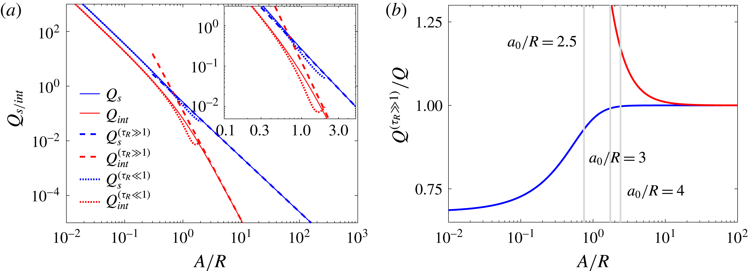
We compare the large- and small-spacing models of the coefficients to the non-approximated terms (2.5) where it is evident that both the large- and small-spacing approximations correspond nicely to the non-approximated terms in each of their respective domains (figure 2
a). It can be observed that for
 $A/R\gg 3$
,
 $Q_{s}/Q_{int}\gg 1$
, which indicates that the dynamics are primarily dictated by the direct term and not by the interaction term. In figure 2(b) we show that the large-scale approximation is valid for most of the
 $A/R$
domain. We plot the ratio
 $Q^{(\unicode[STIX]{x1D70F}_{R}\gg 1)}/Q$
versus
 $A/R$
for both the s and int terms. It can be observed when
 $a_{0}/R\geqslant 3$
that the s ratio is unity while the int ratio departs slightly prior to that. Combined, these findings explain why the dipole model works well even at remarkably small spacing, such as
 $a_{0}/R=4$
, where one does not expect the dipole interaction assumption to hold.
(a) Log–log plot of the various models of coefficients
 $Q_{s}$
and
 $Q_{int}$
versus
 $A/R$
. (Inset) A zoom of (a). (b) Semi-log plot of the ratio of the large-spacing model to the exact model,
 $Q^{(\unicode[STIX]{x1D70F}_{R}\gg )1}/Q$
, versus
 $A/R$
(
 $Q_{s}^{(\unicode[STIX]{x1D70F}_{R}\gg 1)}$
, blue;
 $Q_{int}^{(\unicode[STIX]{x1D70F}_{R}\gg 1)}$
, red). The vertical grey lines mark
 $a_{0}/R=2.5$
, 3 and 4.
4 Two-droplet velocity and perturbation equations
In this section we derive the zeroth-order equation, from which we calculate the droplet velocity,
 $U_{d}$
, and the first-order correction for the perturbation dynamics.
4.1 Large spacing
The
 $a^{-2}$
term in (3.3) can be rewritten (using (2.7)) as
 $a^{-2}\approx (1-2\unicode[STIX]{x0394}\unicode[STIX]{x1D6FF}x/a_{0})a_{0}^{-2}$
. Inserting this relation and (3.3) into (2.1) (
 $F_{i}=0$
) yields two equations of orders
 $O(1)$
and
 $O(\unicode[STIX]{x1D6FF}x/a_{0})$
, respectively:
 $$\begin{eqnarray}\displaystyle & \displaystyle U_{d}^{(\unicode[STIX]{x1D70F}_{R}\gg 1)}=\frac{a_{0}^{2}-R^{2}}{a_{0}^{2}(1+\unicode[STIX]{x1D702})/2-R^{2}}U_{\infty }, & \displaystyle\end{eqnarray}$$
 $$\begin{eqnarray}\displaystyle & \displaystyle -\unicode[STIX]{x1D6FF}{\dot{x}}_{i}(1+\unicode[STIX]{x1D702})+2\unicode[STIX]{x1D6FF}{\dot{x}}_{l}\frac{R^{2}}{a_{0}^{2}}=-4\left[U_{\infty }-U_{d}^{(\unicode[STIX]{x1D70F}_{R}\gg 1)}\right]\frac{R^{2}}{a_{0}^{2}}\frac{\unicode[STIX]{x0394}\unicode[STIX]{x1D6FF}x}{a_{0}}. & \displaystyle\end{eqnarray}$$
To compare with the dipole model, we derived the two-droplet velocity based on the dipole model formulation (Beatus et al.
Reference Beatus, Tlusty and Bar-Ziv2006, Reference Beatus, Bar-Ziv and Tlusty2012). The results are similar; however, the
 $\unicode[STIX]{x1D6FF}{\dot{x}}_{l}R^{2}a_{0}^{-2}$
term in (4.2) is new relative to the dipole model and is discussed later (§ 5.2). We also report an error in the reported expression for the velocity of an infinite lattice (discussed in § 5.2).
Finally, we recall that the parameter
 $\unicode[STIX]{x1D702}$
needs to be calibrated experimentally relative to isolated droplets
 $U_{d}^{(\unicode[STIX]{x1D70F}_{R}\gg 1)}(a_{0}\rightarrow \infty )=2U_{\infty }(1+\unicode[STIX]{x1D702})$
. In this work we use the experimental parameters given in figure 3 of Beatus et al. (Reference Beatus, Tlusty and Bar-Ziv2006),
 $\tilde{R}=10~\unicode[STIX]{x03BC}\text{m}$
,
 $\tilde{U} _{d}(a_{0}\rightarrow \infty )=295~\unicode[STIX]{x03BC}\text{m}~\text{s}^{-1}$
and
 $\tilde{U} _{\infty }=1090~\unicode[STIX]{x03BC}\text{m}~\text{s}^{-1}$
, which yields
 $\unicode[STIX]{x1D702}=2\tilde{U} _{\infty }/\tilde{U} _{d}-1\approx 6.36$
.
4.2 Small spacing
Equation (2.1) yields two equations of order
 $O(1)$
and
 $O(\unicode[STIX]{x1D6FF}xR/A^{2})$
, respectively:
 $$\begin{eqnarray}\displaystyle & \displaystyle U_{d}^{(\unicode[STIX]{x1D70F}_{R}\ll 1)}=\frac{\unicode[STIX]{x03C0}^{2}}{\unicode[STIX]{x03C0}^{2}-6+6\unicode[STIX]{x1D702}}U_{\infty }, & \displaystyle\end{eqnarray}$$
 $$\begin{eqnarray}\displaystyle & \displaystyle -3(4\unicode[STIX]{x1D702}+\unicode[STIX]{x03C0}^{2}-4)\unicode[STIX]{x1D6FF}{\dot{x}}_{i}+\unicode[STIX]{x03C0}^{2}\unicode[STIX]{x1D6FF}{\dot{x}}_{l}=0. & \displaystyle\end{eqnarray}$$
Equation (4.3) is a novel lower bound for the droplet velocity. Equation (4.4) has the trivial solution,
 $\unicode[STIX]{x1D6FF}x_{i}(t)=\unicode[STIX]{x1D6FF}x_{i}(t=0)$
, indicating that the droplet dynamics are quasi-stable.
4.3 Droplet velocity comparison
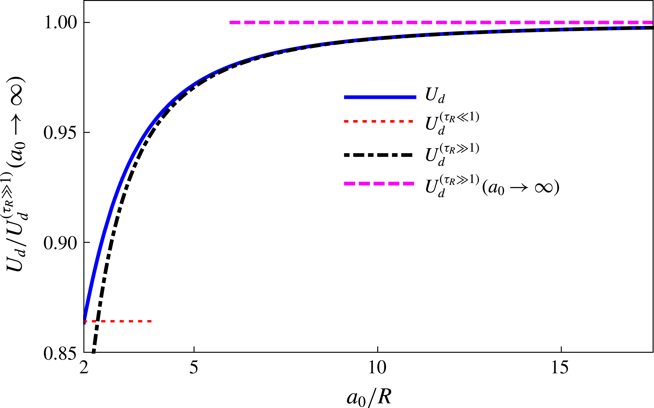
In figure 3 we plot the various models for the velocity as a function of droplet spacing. The non-approximated solution varies between the upper,
 $U_{d}^{(\unicode[STIX]{x1D70F}_{R}\gg 1)}(a_{0}\rightarrow \infty )$
, and lower,
 $U_{d}^{(\unicode[STIX]{x1D70F}_{R}\ll 1)}$
, constant approximations. We see that the large-spacing approximation is valid for most spacing. This is no longer surprising, as discussed in § 3.3.




5
 $N>2$
and infinite lattices

5.1 Extension from
$N=2$
to
$N>2$


We know from Beatus et al. (Reference Beatus, Tlusty and Bar-Ziv2006) that, even when the no-flux BC is not satisfied, the dipole model corresponds very well to the experimental results for large spacing. In § 3.3, we showed that the effects of the interactions are not dominant if
 $a_{0}\gg R$
. This suggests that our
 $N=2$
model can be extended to
 $N>2$
where we acknowledge that such a system would not satisfy the no-flux BC. As we will show, the effects appear to be negligible. The extension of our mechanical equilibrium model to
 $N>2$
droplet lattices using the superposition method is similar to the dipole model, yet our derivation differs in that we model the forces and do not use a predetermined velocity potential. An added advantage of our method is that in § 4.1 we showed that our model predicts an additional term that does not exist in the traditional dipole model. We will analyse the effect of this term. In what will follow, we focus only on large spacing,
 $\unicode[STIX]{x1D70F}_{R}\gg 1$
, and for the sake of brevity and clarity, we drop all superscripts.
Our starting point is to require mechanical equilibrium such that each droplet satisfies
 $F_{direct}+F_{int,i}(N)=0$
. While
 $F_{direct}$
is spacing- and
 $N$
-independent (3.3),
 $F_{int,i}$
depends on both. Thus we rewrite the interaction force for the
 $i\text{th}$
droplet to account for all interactions:
 $$\begin{eqnarray}F_{int,i}(N)=\mathop{\sum }_{l\neq i}^{N}F_{int,i-l}.\end{eqnarray}$$
To write out
 $F_{int,i-l}$
explicitly, we need to know the
 $a_{il}$
spacings, which are given by
 $$\begin{eqnarray}\displaystyle & \displaystyle a_{il}(t)=a_{0,il}+\unicode[STIX]{x0394}\unicode[STIX]{x1D6FF}x_{\left\{i,l\right\}}, & \displaystyle\end{eqnarray}$$
 $$\begin{eqnarray}\displaystyle & \displaystyle a_{0,il}(t)=\left|i-l\right|a_{0}, & \displaystyle\end{eqnarray}$$
 $$\begin{eqnarray}\displaystyle & \displaystyle \unicode[STIX]{x0394}\unicode[STIX]{x1D6FF}x_{\left\{i,l\right\}}=\left\{\begin{array}{@{}ll@{}}\unicode[STIX]{x1D6FF}x_{i}-\unicode[STIX]{x1D6FF}x_{l}, & i>l,\\ \unicode[STIX]{x1D6FF}x_{l}-\unicode[STIX]{x1D6FF}x_{i}, & i<l.\end{array}\right. & \displaystyle\end{eqnarray}$$
Equation (5.3) ensures that all the droplets are evenly spaced similar as in a solid-state crystal (Kittel Reference Kittel1986). Equation (5.4) ensures that the sign of the perturbation difference in (5.2) is self-consistent for each equation. In the interaction force, we are primarily interested in
 $a_{il}^{-2}$
. The approximation yields
 $$\begin{eqnarray}\frac{1}{a_{il}^{2}}\cong \frac{1-2\unicode[STIX]{x0394}\unicode[STIX]{x1D6FF}x_{\left\{i,l\right\}}/(a_{0}\left|i-l\right|)}{a_{0}^{2}(i-l)^{2}}.\end{eqnarray}$$
As in § 4, we shall need to divide the forces into zeroth- and first-order terms, which are denoted by the respective superscripts
 $O(1)$
and
 $O(\unicode[STIX]{x1D6FF}x)$
:
 $$\begin{eqnarray}\displaystyle & \displaystyle F_{int,i-l}^{O(1)}=\frac{F_{2,l}}{(i-l)^{2}}, & \displaystyle\end{eqnarray}$$
 $$\begin{eqnarray}\displaystyle & \displaystyle F_{int,i-l}^{O(\unicode[STIX]{x1D6FF}x)}=\frac{2\unicode[STIX]{x03C0}R^{4}}{a_{0}^{2}(i-l)^{2}}\unicode[STIX]{x1D6FF}{\dot{x}}_{l}-2\frac{F_{2,l}}{(i-l)^{2}}\frac{\unicode[STIX]{x0394}\unicode[STIX]{x1D6FF}x_{\left\{i,l\right\}}}{a_{0}\left|i-l\right|}, & \displaystyle\end{eqnarray}$$
where
 $F_{2,l}=2\unicode[STIX]{x03C0}(U_{d,l}-U_{\infty })R^{4}/a_{0}^{2}$
is the zeroth-order term of the two-droplet case (3.3). The subscript
 $l$
indicates that this coefficient changes if one does not make the explicit assumption that the droplets move with a uniform velocity
 $(U_{d,l}=U_{d})$
. Since an infinite lattice has a fore–aft symmetry, we make that assumption and drop this subscript,
 $F_{2,l}=F_{2}$
.
5.2 Infinite lattice
In this section we shall reproduce the results of Beatus et al. (Reference Beatus, Tlusty and Bar-Ziv2006) for an infinite lattice. The zeroth-order expression from (5.1) yields
 $$\begin{eqnarray}F_{int}^{O(1)}(N\rightarrow \infty )=\mathop{\sum }_{l=-\infty ,l\neq i}^{\infty }F_{int,i-l}^{O(1)}=\mathop{\sum }_{l=-\infty ,l\neq i}^{\infty }\frac{F_{2}}{(i-l)^{2}}=2F_{2}\mathop{\sum }_{l=1}^{\infty }l^{-2}=2\left(\frac{\unicode[STIX]{x03C0}^{2}}{6}\right)F_{2},\end{eqnarray}$$
where we have already encountered this infinite sum. The zeroth-order force balance yields the velocity
 $$\begin{eqnarray}U_{d}=\frac{a_{0}^{2}-(\unicode[STIX]{x03C0}^{2}/3)R^{2}}{(1+\unicode[STIX]{x1D702})a_{0}^{2}/2-(\unicode[STIX]{x03C0}^{2}/3)R^{2}}U_{\infty }.\end{eqnarray}$$
Equation (5.9) has a similar form to (4.1) except that the
 $R^{2}$
coefficient is now
 $\unicode[STIX]{x03C0}^{2}/3$
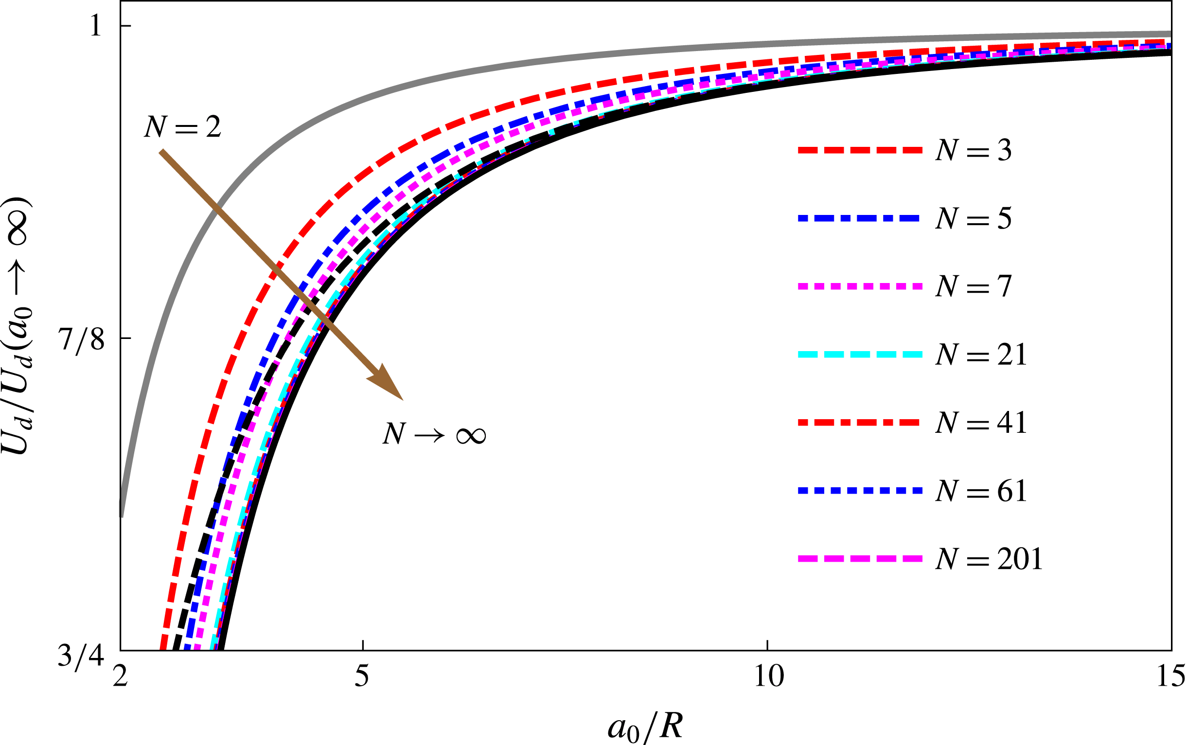
instead of 1. Later, in figure 5, we compare the two-droplet case to the infinite lattice. It can be observed that, for a given spacing, the two-droplet system (solid grey line) has a higher velocity than the infinite lattice (solid black line). As the number of droplets increases, so does the number of interaction forces, resulting in an increase in the total interaction force, which operates as an effective drag. This results in a decrease of the velocity with increasing
 $N$
, for constant spacing. This explanation and that
 $U_{d}(N=2)>U_{d}(N\rightarrow \infty )$
conflict with the original ‘peloton effect’ explanation of Beatus et al. (Reference Beatus, Tlusty and Bar-Ziv2006, Reference Beatus, Bar-Ziv and Tlusty2012) that compared the infinite lattice to riding cyclists. Indeed, cyclists riding in the turbulent wake of preceding cyclists can pedal less and stay at the same velocity; however, drag reduction is a large-Reynolds-number effect, related to boundary layer effects, that has no equivalent in classical low-Reynolds-number Hele-Shaw flows.
Equation (5.9) differs from that given in Beatus et al. (Reference Beatus, Tlusty and Bar-Ziv2006),
 $$\begin{eqnarray}U_{d}^{(dipole)}=\frac{a_{0}^{2}U_{d}^{(dipole,\infty )}}{a_{0}^{2}+\unicode[STIX]{x03C0}^{2}R^{2}(1-U_{d}^{(dipole,\infty )}/U_{\infty })/3},\end{eqnarray}$$
where
 $U_{d}^{(dipole,\infty )}=U_{\infty }(1+\unicode[STIX]{x1D707}_{dipole}/\unicode[STIX]{x1D709}_{d})^{-1}$
is the velocity of an isolated particle,
 $\unicode[STIX]{x1D707}_{dipole}$
is similar to our
 $\unicode[STIX]{x1D702}$
, in the sense that it is a fitting parameter, and
 $\unicode[STIX]{x1D709}_{d}=\unicode[STIX]{x1D709}_{d}(\unicode[STIX]{x1D707},R,h)$
was a drag parameter. Beatus et al. (Reference Beatus, Tlusty and Bar-Ziv2006, Reference Beatus, Bar-Ziv and Tlusty2012) made an error in their final calculation. If one follows the derivation as prescribed in their works, one gets
 $$\begin{eqnarray}U_{d}^{(corrected~dipole)}=\frac{a_{0}^{2}-(\unicode[STIX]{x03C0}^{2}/3)R^{2}}{a_{0}^{2}(U_{\infty }/{U_{d}}^{(dipole,\infty )})-(\unicode[STIX]{x03C0}^{2}/3)R^{2}}U_{\infty },\end{eqnarray}$$
where it is now evident that (5.11) is similar in form to (5.9) when
 $a_{0}\gg R$
. In figure 5 we compare our infinite lattice (solid black line) and that of Beatus et al. (Reference Beatus, Tlusty and Bar-Ziv2006, Reference Beatus, Bar-Ziv and Tlusty2012) (dashed black line). It is likely that Beatus et al. (Reference Beatus, Tlusty and Bar-Ziv2006, Reference Beatus, Bar-Ziv and Tlusty2012) did not pick up their error because the functional forms of (5.9)–(5.11) are similar and matched experiments.
We now investigate the perturbation equations. Using
 $F_{int,i-l}^{O(\unicode[STIX]{x1D6FF}x)}$
(5.7) and
 $F_{direct}^{O(\unicode[STIX]{x1D6FF}x)}$
(3.3) yields
 $$\begin{eqnarray}-(1+\unicode[STIX]{x1D702})\unicode[STIX]{x1D6FF}{\dot{x}}_{i}+\mathop{\sum }_{l=-\infty ,l\neq i}^{\infty }\frac{2}{(i-l)^{2}}\left[\frac{\unicode[STIX]{x1D6FF}{\dot{x}}_{l}R^{2}}{a_{0}^{2}}-\frac{F_{2}\unicode[STIX]{x0394}\unicode[STIX]{x1D6FF}x_{\left\{i,l\right\}}}{\unicode[STIX]{x03C0}R^{2}a_{0}\left|i-l\right|}\right]=0.\end{eqnarray}$$
This equation differs from the dipole model perturbation equation (Beatus et al.
Reference Beatus, Tlusty and Bar-Ziv2006, Reference Beatus, Bar-Ziv and Tlusty2007, Reference Beatus, Bar-Ziv and Tlusty2012), whereby our model includes the
 $\sum \unicode[STIX]{x1D6FF}{\dot{x}}_{l}$
coupling correction. For simplicity we neglect this term for now, as we reproduce the classical results of the dipole model. We shall add its effects hereafter. We rewrite (5.12) as
 $$\begin{eqnarray}\unicode[STIX]{x1D6FF}{\dot{x}}_{\hat{i} =0}=-C_{s}\mathop{\sum }_{l=-\infty ,l\neq 0}^{\infty }\frac{\unicode[STIX]{x0394}\unicode[STIX]{x1D6FF}x_{\left\{\hat{i} =0,l\right\}}}{|l|^{3}}=-C_{s}\mathop{\sum }_{l=1}^{\infty }\frac{\unicode[STIX]{x0394}\unicode[STIX]{x1D6FF}x_{\left\{0,l\right\}}+\unicode[STIX]{x0394}\unicode[STIX]{x1D6FF}x_{\left\{0,-l\right\}}}{l^{3}}=C_{s}\mathop{\sum }_{l=1}^{\infty }\frac{\unicode[STIX]{x1D6FF}x_{l}-\unicode[STIX]{x1D6FF}x_{-l}}{l^{3}},\end{eqnarray}$$
where
 $C_{s}=4R^{2}(U_{\infty }-U_{d})/[a_{0}^{3}(1+\unicode[STIX]{x1D702})]$
. We insert a travelling wave,
 $\unicode[STIX]{x1D6FF}x_{i}\sim \exp [\text{j}(kx-\unicode[STIX]{x1D714}t)]$
, into (5.13) (
 $\text{j}=\sqrt{-1}$
is the imaginary number). The droplet with subscript
 $l$
is located at
 $x=la_{0}$
. After some algebraic manipulations (5.13) yields
 $$\begin{eqnarray}\unicode[STIX]{x1D714}_{\infty }=-2C_{s}\mathop{\sum }_{l=1}^{\infty }\frac{\sin (lka_{0})}{l^{3}}.\end{eqnarray}$$
The infinity subscript has been added to indicate an infinite lattice
 $(N\rightarrow \infty )$
. Equation (5.14) has the same form as that of the original work (Beatus et al.
Reference Beatus, Tlusty and Bar-Ziv2006, Reference Beatus, Bar-Ziv and Tlusty2012) save for the fitting parameter
 $\unicode[STIX]{x1D702}$
. We report that this infinite series converges to a simple polynomial of order 3 (see equation 1.443-5 on p. 47 of Gradshteyn & Ryzhik (Reference Gradshteyn and Ryzhik2007)):
 $$\begin{eqnarray}\mathop{\sum }_{l=1}^{\infty }\frac{\sin (lka_{0})}{l^{3}}=\frac{\unicode[STIX]{x03C0}^{2}ka_{0}}{6}-\frac{\unicode[STIX]{x03C0}(ka_{0})^{2}}{4}+\frac{(ka_{0})^{3}}{12},\quad 0\leqslant ka_{0}\leqslant 2\unicode[STIX]{x03C0}.\end{eqnarray}$$
Note that the coefficient of the linear term is the previously encountered
 $\unicode[STIX]{x03C0}^{2}/6$
similar to that in (3.5), (3.6) and (5.8) – the importance of which will become apparent soon. We return to the previously neglected coupling term in (5.12). Inserting the travelling wave into it yields
 $$\begin{eqnarray}2\frac{R^{2}}{a_{0}^{2}}\mathop{\sum }_{l=-\infty ,l\neq 0}^{\infty }\frac{\unicode[STIX]{x1D6FF}{\dot{x}}_{l}}{l^{2}}=-2\text{j}\unicode[STIX]{x1D714}\text{e}^{-\text{j}\unicode[STIX]{x1D714}t}\frac{R^{2}}{a_{0}^{2}}\mathop{\sum }_{l=1}^{\infty }\frac{\text{e}^{\text{j}kla_{0}}+\text{e}^{-\text{j}kla_{0}}}{l^{2}}=-\text{j}\unicode[STIX]{x1D701}\unicode[STIX]{x1D714}\text{e}^{-\text{j}\unicode[STIX]{x1D714}t},\end{eqnarray}$$
where
 $\unicode[STIX]{x1D701}=2R^{2}[Li_{2}(\text{j}ka_{0})+Li_{2}(-\text{j}ka_{0})]a_{0}^{-2}$
is a real number, and
 $Li_{2}(\unicode[STIX]{x1D703})=\sum _{l=1}^{\infty }\unicode[STIX]{x1D703}^{l}l^{-2}$
is the polylogarithm of order 2 and argument
 $\unicode[STIX]{x1D703}$
(Lewin Reference Lewin1991). Inserting (5.16) into (5.13) would modify (5.14) such that
 $\unicode[STIX]{x1D714}_{\infty ,corrected}=\unicode[STIX]{x1D714}_{\infty }(1+\unicode[STIX]{x1D702})/(1+\unicode[STIX]{x1D702}-\unicode[STIX]{x1D701})$
. In figure 4 we plot the ratio
 $\unicode[STIX]{x1D714}_{\infty ,corrected}/\unicode[STIX]{x1D714}_{\infty }$
for various values of
 $a_{0}/R$
. Naturally, as the droplets are spaced farther apart, the correction is of less importance, yet, for closely packed droplets, the correction can be 4–6 %.
Plot of
 $\unicode[STIX]{x1D714}_{\infty ,corrected}/\unicode[STIX]{x1D714}_{\infty }$
versus the normalized wave number
 $ka_{0}$
for different
 $a_{0}/R$
ratios and
 $\unicode[STIX]{x1D702}=6.36$
.

5.3 The finite
$N$
-droplet lattice

In the previous section we showed that the zeroth-order term of the total interaction force was multiplied by
 $\unicode[STIX]{x03C0}^{2}/3$
relative to the case of two droplets. We expect that this remains true also for a finite but large number of droplets. In reality, in a finite numbered lattice, the total interaction force on edge droplets is different from those near the centre. It can be shown that the ratio is at most a factor of 2. With this understanding, combined with the previous understanding, the interaction force is not the dominant force in the system; we make a simplifying assumption that all droplets behave as a droplet located at the centre. We shall show that, even for relatively small
 $N$
, the lattice will behave in a very similar way to an infinite lattice. Hence we continue to require that
 $U_{d,i}=U_{d}$
.
For the case of an odd number of droplets,
 $N=2M+1$
(
 $M$
pairs relative to the central droplet), the total interaction force is straightforward:
 $$\begin{eqnarray}F_{int}^{O(1)}(2N+1)=2F_{2}\mathop{\sum }_{l=1}^{M}l^{-2}=G_{M}F_{2},\end{eqnarray}$$
where
 $G_{M}=2\sum _{l=1}^{M}l^{-2}=2H_{M,2}$
and
 $H_{M,2}$
is the generalized harmonic number of order
 $M$
of power 2. As can be expected,
 $H_{M\rightarrow \infty ,2}\rightarrow \unicode[STIX]{x03C0}^{2}/6$
. Like the infinite lattice, it can be shown that the droplet velocity is
 $$\begin{eqnarray}U_{d}=\frac{a_{0}^{2}-G_{M}R^{2}}{(1+\unicode[STIX]{x1D702})a_{0}^{2}/2-G_{M}R^{2}}U_{\infty }.\end{eqnarray}$$
Equation (5.18) has a similar form to (4.1) and (5.9). Already for small lattices (
 $G_{10}/G_{\infty }\sim 94\,\%$
), the lattice is practically infinite and edge effects can be ignored.
In figure 5 we plot the droplet velocity versus the spacing for a travelling lattice of
 $N$
droplets. As
 $N$
increases, equation (5.18) varies monotonically from its
 $N=2$
lower limit (4.1) to its
 $N\rightarrow \infty$
upper limit (5.9). As can be expected, already at
 $N=21$
the lattice behaves as an almost infinite lattice, justifying the assumption
 $U_{d,i}=U_{d}$
.
Normalized droplet velocity
 $U_{d}/U_{d}(a_{0}\rightarrow \infty )$
versus
 $a_{0}/R$
for varying number of droplets. The brown arrow points in the direction of increasing
 $N$
. The two extreme cases of
 $N=2$
(4.1) and
 $N\rightarrow \infty$
(5.9) are marked by a solid grey and black line, respectively. The black dashed line is the velocity (5.10) given by Beatus et al. (Reference Beatus, Tlusty and Bar-Ziv2006, Reference Beatus, Bar-Ziv and Tlusty2012).
Similarly, the perturbation equation for finite
 $N$
is
 $$\begin{eqnarray}-(1+\unicode[STIX]{x1D702})\unicode[STIX]{x1D6FF}{\dot{x}}_{i}+\mathop{\sum }_{l\neq i}^{2M+1}\frac{2}{(i-l)^{2}}\left[\frac{\unicode[STIX]{x1D6FF}{\dot{x}}_{l}R^{2}}{a_{0}^{2}}-\frac{F_{2}\unicode[STIX]{x0394}\unicode[STIX]{x1D6FF}x_{\left\{i,l\right\}}}{\unicode[STIX]{x03C0}R^{2}a_{0}\left|i-l\right|}\right]=0.\end{eqnarray}$$
For simplicity, we neglect the new correction term, which yields the following dispersion relation:
 $$\begin{eqnarray}\unicode[STIX]{x1D714}_{N}=-2C_{s}\mathop{\sum }_{l=1}^{M}\frac{\sin (lka_{0})}{l^{3}}.\end{eqnarray}$$
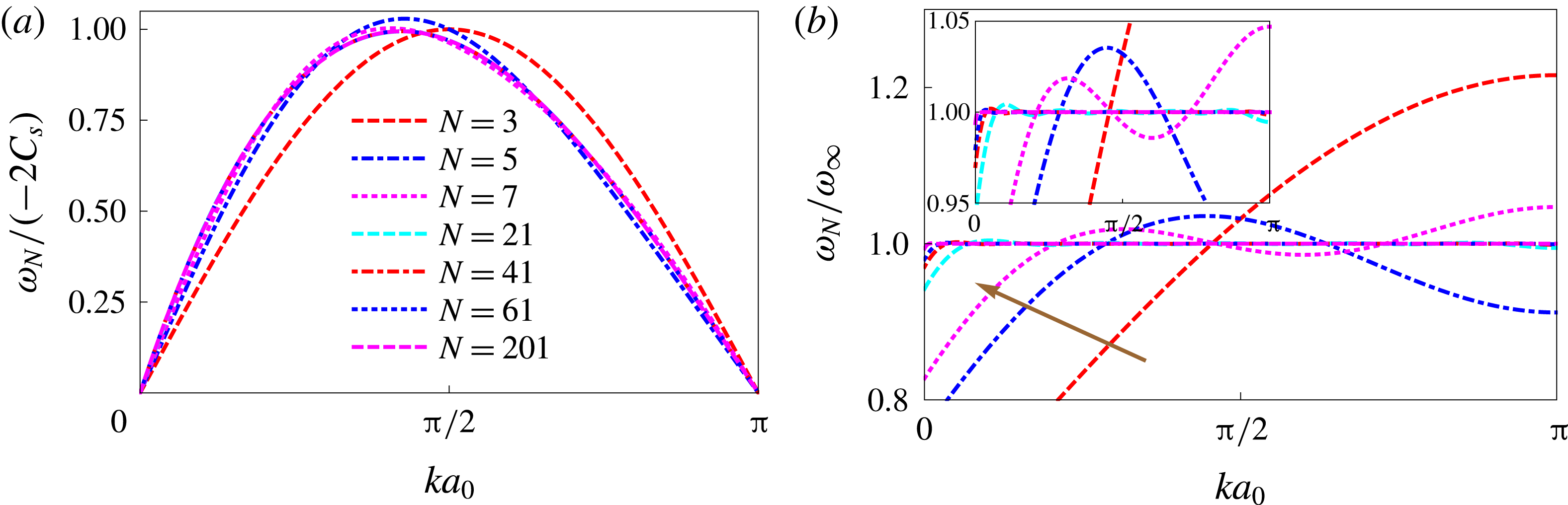
In figure 6(a) we plot the ratio
 $-\unicode[STIX]{x1D714}_{N}/2C_{s}$
versus the normalized wavenumber
 $ka_{0}$
for varying
 $N$
. As the number of droplets increases, the solution converges to the infinite solution. It converges faster than the droplet velocity convergence because
 $\unicode[STIX]{x1D714}_{N}$
converges as
 $l^{-3}$
while
 $G_{M}$
converges as
 $l^{-2}$
. It can be seen in figure 6(b) that
 $N=3$
(two nearest-neighbour interactions) given by the dashed red line accounts for approximately 80 % of the
 $\unicode[STIX]{x1D714}_{\infty }$
response. Also, at relatively small numbers, such as
 $N\sim O(20)$
, the ratio is unity for almost all
 $ka_{0}$
. However, it can be observed that the solution does not converge at small
 $ka_{0}$
(large wavelengths) even for large
 $N$
. This is rationalized based on a previous observation: the linear term of the dispersion relation (5.15) with the coefficient
 $\unicode[STIX]{x03C0}^{2}/6$
is determined by an infinite number of interactions. Simply put: a finite-sized lattice can sustain only a finite-sized wavelength.
(a) A plot of
 $-\unicode[STIX]{x1D714}_{N}/2C_{s}$
versus the normalized wavenumber
 $ka_{0}$
for a system of varying droplet number,
 $N$
. (b) A plot of the ratio
 $\unicode[STIX]{x1D714}_{N}/\unicode[STIX]{x1D714}_{\infty }$
versus the normalized wavenumber
 $ka_{0}$
. (Inset) A zoom of (b). The brown arrow indicates direction of increasing
 $N$
.
6 Conclusions
In this work we have shown that using the large- and small-spacing approximations of the Fourier coefficients (2.5) allows the zeroth- and first-order governing equations to be written out in simple form. This allows for additional analysis that is not possible with the non-approximated series. While this model recapitulates much of the results of the dipole model, it is different in that it does not use a predetermined flow potential and dictates the interaction to be dipolar. Rather, the dipolar interaction is a result. Further, the analysis is based on the assumption of mechanical equilibrium. Also, a new term, which does not exist in the dipole, appears. The discussion here follows the structure of this paper. We will first focus on the
 $N=2$
findings and then move to the
 $N>2$
findings.
In § 3 we investigated the interplay between the various forces for
 $N=2$
droplets. There, we showed that
 $Q_{s}\gg Q_{int}$
, when
 $a_{0}/R>3$
, so that the effect of the interaction term is relatively negligible compared to the other forces such that dynamics are primarily determined by
 $F_{direct}$
. We further show that the dipole model solution corresponds to the non-approximated velocity in most of the
 $a_{0}/R$
domain, even at relatively small spacings where it is expected to fail (figure 3).
Thus far, the small-spacing approximation appears not to have received much attention in the literature. This is perhaps because it was assumed that if the interaction is not dipolar, the mathematical complexity increases, and perhaps that the Hele-Shaw approximation would fail. Sarig et al. (Reference Sarig, Starosvetsky and Gat2016) compared their results with the experiments of Shen et al. (Reference Shen, Leman, Reyssat and Tabeling2014) and the correspondence was striking, indicating that the Hele-Shaw approximation holds. Further, our small-spacing solution provides a simple estimate,
 $U_{d}^{(\unicode[STIX]{x1D70F}_{R}\ll 1)}$
(4.3).
Both the small- and large-spacing approximations have the potential to solve related problems. The formulation here can be extended to two dimensions, and/or can solve for non-identical droplets (Sarig et al. Reference Sarig, Starosvetsky and Gat2016). In appendix A we extend the large-spacing approximation for non-identical droplets. Also, Sarig et al. (Reference Sarig, Starosvetsky and Gat2016) suggested that the model is also suitable for investigating the dynamics of a small droplet encapsulated in a larger droplet. The Fourier coefficients for such a scenario are almost the same as those discussed in this work. Hence, with some modifications, this too can be solved. These approximations can also be extended to investigate the well-known Villat formula. It would be interesting to see if that flow potential can be reduced to a simpler expression for large and small approximations.
The exact details of the friction coefficient are currently unknown. We have suggested a new form for the friction coefficient. It would be interesting and helpful to conduct a thorough experimental investigation of the velocity of an isolated drop
 $U_{d}(a_{0}\rightarrow \infty )$
as a function of the parameters
 $U_{\infty },R,h,\tilde{\unicode[STIX]{x1D707}}_{f},\tilde{\unicode[STIX]{x1D707}}_{d},\tilde{\unicode[STIX]{x1D70E}}$
as they are varied.
Finally, in § 5 we extended the derivation from
 $N=2$
to
 $N>2$
droplets. For a given spacing, as
 $N$
increases,
 $U_{d}$
decreases. This is due to the increase of the effective drag. The velocity converges with increasing
 $N$
to the infinite solution. For the dispersion relation,
 $\unicode[STIX]{x1D714}_{N}$
, we show that already at relatively small
 $N\sim O(20)$
the finite lattice behaves as an infinite lattice save for a small discrepancy at small
 $ka_{0}$
. We also investigate the behaviour of the new
 $O(R^{2}/a^{2})$
correction to the dispersion relation and show that it introduces a correction of a few per cent. In this work, we have started to investigate the effect of this term and we have shown that the new term leads to a few per cent change in the dispersion relation. Yet, it would indeed be interesting to see how this term might effect the long-time evolution of non-crystal-like lattices that have been investigated numerically and experimentally (Liu et al.
Reference Liu, Goree and Feng2012; Shen et al.
Reference Shen, Leman, Reyssat and Tabeling2014). It would indeed be interesting to investigate the case of a lattice of
 $N>2$
where all droplets are touching. On the one hand, we know that all non-nearest-neighbour dynamics
 $(a_{ij}>4R)$
can be modelled by dipolar interactions, yet it is unclear how the nearest-neighbour interactions
 $(a_{min}=2R)$
should be modelled. This is left for future work.
Acknowledgements
We thank A. Gat, Y. Starosvetsky and I. Sarig for fruitful discussions and helpful comments. We thank the anonymous referees for their insightful comments; notably the referee who pointed us to the Poisson summation formula, which vastly simplified our calculations for the small-spacing approximation.
Appendix A. Two-droplet generalizations
Sarig et al. (Reference Sarig, Starosvetsky and Gat2016) solved the case of two droplets of arbitrary radii and viscosities. For this general case, the
 $Q$
coefficients have a more complicated form:
 $$\begin{eqnarray}\displaystyle & \displaystyle Q_{s}=\mathop{\sum }_{n=1}^{\infty }n\text{e}^{-2n\left|\unicode[STIX]{x1D70F}_{i}\right|}\coth [n(\left|\unicode[STIX]{x1D70F}_{i}\right|+\left|\unicode[STIX]{x1D70F}_{l}\right|)], & \displaystyle\end{eqnarray}$$
 $$\begin{eqnarray}\displaystyle & \displaystyle Q_{int}=\mathop{\sum }_{n=1}^{\infty }n\text{e}^{-n(\left|\unicode[STIX]{x1D70F}_{i}\right|+\left|\unicode[STIX]{x1D70F}_{l}\right|)}\,\text{csch}[n(\left|\unicode[STIX]{x1D70F}_{i}\right|+\left|\unicode[STIX]{x1D70F}_{l}\right|)], & \displaystyle\end{eqnarray}$$
 $$\begin{eqnarray}\displaystyle & \displaystyle A=(2a)^{-1}\sqrt{[a^{2}-(R_{1}+R_{2})^{2}][a^{2}-(R_{1}-R_{2})^{2}]}, & \displaystyle\end{eqnarray}$$
 $$\begin{eqnarray}\displaystyle & \displaystyle \unicode[STIX]{x1D70F}_{1,2}=\pm \,\text{sinh}^{-1}(A/R_{1,2}). & \displaystyle\end{eqnarray}$$
For the case of large spacing, when
 $a\gg R_{1}+R_{2}$
(
 $A=a/2$
and
 $\left|\unicode[STIX]{x1D70F}_{i}\right|=\log (a/R_{i})$
):
 $$\begin{eqnarray}\displaystyle & \displaystyle Q_{s}^{(\unicode[STIX]{x1D70F}_{R}\gg 1)}=\mathop{\sum }_{n=1}^{\infty }n\text{e}^{-2n\left|\unicode[STIX]{x1D70F}_{i}\right|}\,\coth \left[n(\left|\unicode[STIX]{x1D70F}_{i}\right|+\left|\unicode[STIX]{x1D70F}_{l}\right|)\right]\approx \mathop{\sum }_{n=1}^{\infty }n\text{e}^{-2n\left|\unicode[STIX]{x1D70F}_{i}\right|}=\frac{\text{e}^{2\unicode[STIX]{x1D70F}_{i}}}{(\text{e}^{2\unicode[STIX]{x1D70F}_{i}}-1)^{2}}\approx \frac{{R_{i}}^{2}}{a^{2}}, & \displaystyle\end{eqnarray}$$
 $$\begin{eqnarray}\displaystyle & \displaystyle Q_{int}^{(\unicode[STIX]{x1D70F}_{R}\gg 1)}=\mathop{\sum }_{n=1}^{\infty }n\text{e}^{-n(|\unicode[STIX]{x1D70F}_{i}|+|\unicode[STIX]{x1D70F}_{l}|)}\,\text{csch}[n(|\unicode[STIX]{x1D70F}_{i}|+|\unicode[STIX]{x1D70F}_{l}|)]\approx \mathop{\sum }_{n=1}^{\infty }2n\text{e}^{-2n(|\unicode[STIX]{x1D70F}_{i}|+|\unicode[STIX]{x1D70F}_{l}|)} & \displaystyle \nonumber\\ \displaystyle & \qquad =\displaystyle \frac{2\text{e}^{2(|\unicode[STIX]{x1D70F}_{i}|+|\unicode[STIX]{x1D70F}_{l}|)}}{[\text{e}^{2(|\unicode[STIX]{x1D70F}_{i}|+|\unicode[STIX]{x1D70F}_{l}|)}-1]^{2}}\approx \displaystyle \frac{2{R_{i}}^{2}{R_{l}}^{2}}{a^{4}}. & \displaystyle\end{eqnarray}$$
From (A 5), it is apparent that the force associated with the
 $Q_{s}$
term is unequal for each droplet, which will lead to
 $F_{direct,1}\neq F_{direct,2}$
such that the droplets move at different velocity
 $(U_{d,i}\neq U_{d})$
. The friction force is also dependent on the radii and viscosity
 $F_{friction,i}=\unicode[STIX]{x03C0}\unicode[STIX]{x1D702}_{i}{R_{i}}^{2}\dot{q}_{i}$
. Inserting all these results into (2.1) will yield an algebraic set of equations for
 $U_{d,i}$
.