





1. Introduction
Peristalsis is a common driving mechanism of fluid flow within our bodies, caused by pulsations that propagate along the walls of conduits (Jaffrin & Shapiro Reference Jaffrin and Shapiro1971). This transport mechanism has been observed in the gastrointestinal tract (Acharya et al. Reference Acharya, Halder, Kou, Kahrilas, Pandolfino and Patankar2022), in the urinary system (Cummings et al. Reference Cummings, Waters, Wattis and Graham2004), in the reproductive tract (Leftwich & Baumer Reference Leftwich and Baumer2024) and in lymphatic vessels (Winn & Katifori Reference Winn and Katifori2024). The glymphatic system (Iliff et al. Reference Iliff2012) provides an intriguing case in which peristaltic transport may arise in complex geometry.
The glymphatic system involves the flow of cerebrospinal fluid (CSF) driven by arterial pulsations within annular conduits called the periarterial space (PAS) (Iliff et al. Reference Iliff2012; Mestre et al. Reference Mestre, Tithof, Du, Song, Peng, Sweeney, Olveda, Thomas, Nedergaard and Kelley2018; Hauglund et al. Reference Hauglund2025). Several features have been observed in in vivo experimental studies. The first feature is that the arteries are often placed off centre within the PASs (Tithof et al. Reference Tithof, Kelley, Mestre, Nedergaard and Thomas2019). The second feature inferred from in vivo flow tracer studies is that the PASs located on the brain surface (pial PAS) are open spaces and those penetrating within the brain tissue (penetrating PAS) are porous (Iliff et al. Reference Iliff2012; Schain et al. Reference Schain, Melo-Carrillo, Strassman and Burstein2017; Bedussi et al. Reference Bedussi, van der Wel, de Vos, van Veen, Siebes, Vanbavel and Bakker2017; Bedussi et al. Reference Bedussi, Almasian, de Vos, VanBavel and Bakker2018; Mestre et al. Reference Mestre, Tithof, Du, Song, Peng, Sweeney, Olveda, Thomas, Nedergaard and Kelley2018). This observation was also supported by the recent PAS morphology characterisation study by Mestre et al. (Reference Mestre2022), which showed that the merging of the epipial and/or intimal pial layers at the entrance of penetrating arterioles formed a porous structure that restricted the entry of large tracer particles. The third feature noted is that the astrocyte endfeet layer is displaced by flow within the PAS, which, in turn, can affect hydraulic resistance in these narrow spaces, thereby presenting a two-way-coupled biomechanical fluid–structure interaction (Heil & Hazel Reference Heil and Hazel2011). Endfeet-layer displacements of
 ${\approx} 1\text{–}1.5\,{ {\textrm {}}}\,{{\unicode[Arial]{x03BC}} {\textrm {m}}}$
and
 ${\approx} 2\,{{\unicode[Arial]{x03BC}} {\textrm {m}}}$
have been observed during functional hyperaemia (Kedarasetti et al. Reference Kedarasetti, Turner, Echagarruga, Gluckman, Drew and Costanzo2020; Holstein-Rønsbo et al. Reference Holstein-Rønsbo2023) and natural sleep–wake variation (Bojarskaite et al. Reference Bojarskaite, Vallet, Bjørnstad, Gullestad Binder, Cunen, Heuser, Kuchta, Mardal and Enger2023), respectively. Given these features, understanding the mechanics of PAS flows requires integrating the principles of peristalsis, transport in porous media and fluid–structure interactions.
To address the first feature of flows in the PAS, Tithof et al. (Reference Tithof, Kelley, Mestre, Nedergaard and Thomas2019) investigated the hydraulic resistance to steady flow through a non-porous annular PAS, focusing on the area ratios, aspect ratios and inner cylinder eccentricities. They determined the resistance by numerically solving the axial momentum equation, subject to no-slip boundary conditions at the inner and outer walls of the PAS. Meanwhile, Carr et al. (Reference Carr, Thomas, Liu and Shang2021) performed numerical studies of the flow driven by sinusoidal waves in open eccentric PAS geometries of domain length equal to twice the wavelength. In parallel, Coenen, Zhang & Sánchez (Reference Coenen, Zhang and Sánchez2021) developed a reduced-order model based on the lubrication approximation to describe flows driven by waves of arbitrary shape in open eccentric PAS. However, both of these works assumed a rigid outer wall. To address the second and third features of flows in the PAS, Kedarasetti et al. (Reference Kedarasetti, Turner, Echagarruga, Gluckman, Drew and Costanzo2020) performed computational fluid–structure interaction simulations of peristalsis in a porous, penetrating PAS domain and showed that modelling the outer wall as rigid led to unrealistic pressure values, highlighting the importance of modelling the outer wall as compliant. Meanwhile, Romanò et al. (Reference Romanò, Suresh, Galie and Grotberg2020) and Gan et al. (Reference Gan, Holstein-Rønsbo, Nedergaard, Boster, Thomas and Kelley2023) developed lubrication models for peristaltic pumping in a perivascular space domain connected to a porous brain tissue domain through a permeable outer wall (i.e. astrocyte endfeet layer). However, both of these works idealise the PAS conduits as concentric. Takagi, Balmforth & Llewellyn Smith (Reference Takagi, Balmforth and Llewellyn Smith2024) considered peristaltic pumping in a non-axisymmetric compliant conduit, specifically an eccentric annulus with porous walls, but focused on the dynamics relevant to marine organisms.
To our knowledge, no two-way-coupled fluid–structure interaction model is currently available for peristalsis in narrow, porous, non-axisymmetric annular conduits under conditions relevant to CSF flows in the PAS. In this work, we address this knowledge gap. In § 2, we derive the governing equations under the lubrication approximation. We employ a perturbation approach to account for changes in resistance due to the propagation of travelling waves along the inner wall and for displacements at the outer wall caused by elastic deformation. The result is a reduced-order two-way-coupled model in the form of a single nonlinear unsteady partial differential equation (PDE) for the axial pressure variation. In § 3, we demonstrate our model on the example case of peristaltic pumping driven by cardiac pulsations in a porous non-axisymmetric penetrating PAS, focusing on understanding how the hydrodynamic resistance, pressure and flow are affected by eccentricity, the Darcy number and the compliance number. We conclude in § 4.
2. Mathematical model under the lubrication approximation
Consider a flow in a finite-length annular conduit with a porous interior and a compliant outer wall, as shown in figure 1. The instantaneous inner and outer radii of the annular conduit are denoted by
 $r_a$
and
 $r_e$
, with corresponding equilibrium values (i.e. in the absence of peristalsis or deformation) being
 $r_0$
and
 $r_{e,0}$
, attained at the reference pressure
 $p_{\textit{ref}}$
. Note that expressing the inner and outer boundaries of the PAS in the given cylindrical coordinate system requires care. Peristalsis causes the inner radius, measured about the artery’s own axis, to vary as
 \begin{align} r_a(z,t) = r_0 [1+\epsilon \mathcal{T}(\kappa z-\omega t)], \end{align}
with the artery’s axis remaining fixed at a radial offset from the coordinate axis. Here,
 $\mathcal{T}(\kappa z-\omega t)$
is a (dimensionless) travelling wave profile characterised by its wavenumber
 $\kappa$
, angular frequency
 $\omega$
and relative (dimensionless) amplitude
 $\epsilon$
. Meanwhile, the changing outer radius,
 $r_e(z, t)$
, is to be determined. The transverse dimension of the conduit is assumed to be much smaller than
 $\kappa ^{-1}$
. The axial length of the conduit is
 $\ell$
. The eccentricity
 $ecc = d/r_0$
is the ratio of the radial offset between the axes of the two cylinders to the inner radius at equilibrium;
 $ecc=0$
corresponds to concentric cylinders, and
 $ecc = (r_{e,0} - r_0)/r_0$
corresponds to the artery making contact with the endfeet layer. Both the inner and outer walls are assumed to be impermeable to the flow. The porosity and permeability of the interior are denoted by
 $\phi$
and
 $\mathfrak{K}$
, respectively. The fluid in the domain has density
 $\rho$
and dynamic viscosity
 $\mu$
.
Schematic of the model porous domain, with non-axisymmetric cross-section
 $\varOmega _{\textit{cs}}$
, and associated mathematical notation. The boundary of each cross-section,
 $\partial \varOmega _{\textit{cs}}$
, consists of the outer wall (‘endfeet layer’ with radius
 $r_e$
with respect to its own axis), which is always centred at the axis, and the inner cylinder (‘artery’ with radius
 $r_a$
with respect to its own axis), which is offset from the former’s axis, leading to a non-axisymmetric space. The offset between the axes of the two walls is
 $d$
along the ray
 $\theta = 0$
.

2.1. Lubrication approximation and axial velocity
We denote dimensional and dimensionless variables, where possible, by lowercase and uppercase letters, respectively. Focusing on the key variables of the problem, we introduce the typical scalings for lubrication theory, i.e. the long-wave approximation for the peristaltic wave (Coenen et al. Reference Coenen, Zhang and Sánchez2021)
 \begin{align} R=\frac {r}{r_0},\quad Z=\kappa z,\quad T=\omega t,\quad V_Z=\frac {v_z}{\epsilon \omega /\kappa },\quad V_R=\frac {v_r}{\epsilon \omega r_0},\quad P= \frac {p-p_{\textit{ref}}}{\mu \epsilon \omega /(\kappa r_0)^2}. \end{align}
The annular flow is assumed to be at small Womersley number,
 $ \textit{Wo}=r_0\sqrt {\rho \omega /\mu }$
, as is typical for flows in the PAS (Boster et al. Reference Boster, Cai, Ladrón-De Guevara, Sun, Zheng, Du, Thomas, Nedergaard, Karniadakis and Kelley2023); note that
 $ \textit{Wo}^2 = \rho \omega r_0^2/\mu$
is the ratio of the unsteady inertial term to the transverse viscous term in the momentum equation. Under the scalings from (2.2), and making the assumptions that
 $ \textit{Wo}^2 \ll 1$
and
 $(\kappa r_0)^2 \ll 1$
(see table 1), the inertial terms and axial viscous forces drop out of the momentum equation, leaving a balance of transverse viscous forces, the axial pressure gradient and the drag from the enclosed porous medium. Further, since
 $P$
is not a function of
 $R$
or
 $\theta$
, we can write
 $V_Z(R,\theta ,Z)=- (\partial P/\partial Z )\hat {V}_Z(R,\theta )$
. Then,
 $\hat {V}_Z(R,\theta )$
solves a boundary-value problem in the cross-section
 \begin{align} \frac {1}{R} \frac {\partial }{\partial R} \left (R \frac {\partial \hat {V}_Z}{\partial R}\right )+\frac {1}{R^2} \frac {\partial ^2 \hat {V}_Z}{\partial \theta ^2} - \frac {1}{Da} \hat {V}_Z=-1, \qquad \hat {V}_Z=0 \;\;\text{on}\;\; \partial \varOmega _{\textit{cs}}, \end{align}
where
 $ \textit{Da}=\mathfrak{K}/(\phi r_0^2)$
is the Darcy number, which quantifies the relative contribution of the porous medium drag (Nield & Bejan Reference Nield and Bejan2017). Here,
 $\partial \varOmega _{\textit{cs}}$
is the boundary of the non-axisymmetric (eccentric annular) domain
 $\varOmega _{\textit{cs}}$
. For our problem,
 $\partial \varOmega _{\textit{cs}}$
consists of two circles. In the outer-wall-centred coordinate system of figure 1, the inner part of
 $\partial \varOmega _{\textit{cs}}$
is therefore the curve
 $R = R_{a,c} = + ecc\,\cos \theta + \sqrt {R_a^2 - ecc^2\sin ^2\theta }$
with
 $R_a = 1+\epsilon \mathcal{T}$
, while the outer part of
 $\partial \varOmega _{\textit{cs}}$
is
 $R=R_e$
, where the form of
 $R_e$
will be discussed in § 2.2. For given (fixed)
 $R_a$
and
 $R_e$
, we solved (2.3) by the finite element method (FEM) using FEniCS 2019.1.0, an open-source computing platform (Logg et al. Reference Logg, Mardal and Wells2012; Alnaes et al. Reference Alnaes, Blechta, Hake, Johansson, Kehlet, Logg, Richardson, Ring, Rognes and Wells2015), as described in Appendix B.1.
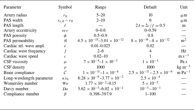
Ranges of dimensional and dimensionless parameters for penetrating PAS flow based on Bloomfield et al. (Reference Bloomfield, Johnston and Bilston1998), Kedarasetti et al. (Reference Kedarasetti, Turner, Echagarruga, Gluckman, Drew and Costanzo2020), Romanò et al. (Reference Romanò, Suresh, Galie and Grotberg2020), Tithof et al. (Reference Tithof, Boster, Bork, Nedergaard, Thomas and Kelley2022), Boster et al. (Reference Boster, Cai, Ladrón-De Guevara, Sun, Zheng, Du, Thomas, Nedergaard, Karniadakis and Kelley2023) and Gan et al. (Reference Gan, Holstein-Rønsbo, Nedergaard, Boster, Thomas and Kelley2023). The brain compliance is estimated as
 $\mathcal{C}\simeq {r_0}/{E_{\textit{endfeet}}}$
, where
 $E_{\textit{endfeet}}\in [10^3, 10^6]$
is an ‘elastic modulus’ in the cited works. The ranges for
 $ \textit{Da}$
and
 $\beta$
are computed by varying
 $\mathfrak{K}$
and
 $\mathcal{C}$
, respectively, over their stated ranges while holding
 $r_0$
,
 $\mu$
,
 $f$
and
 $c$
at their default values, rounding the range edge points where appropriate. The
 $ecc$
range is obtained by varying the axes offset
 $d$
from
 $d=0$
(axisymmetric case, corresponding to
 $ecc=0$
) to
 $d=r_{e,0}-r_0$
(contact with outer wall, corresponding to
 $ecc=0.6$
, which is approached but not attained).

Table 1. Long description
A table with 17 rows and 5 columns detailing the ranges of various parameters for penetrating PAS flow. The columns are labeled Parameter, Symbol, Range, Default, and Unit. Each row lists a specific parameter such as Artery radius, PAS width, PAS length, and so on, along with their respective symbols, ranges, default values, and units. The table provides a comprehensive overview of the dimensional and dimensionless parameters involved in the study of penetrating PAS flow.
Figure 2 shows several solutions for the
 $\hat {V}_Z$
profile for different pairs of
 $ecc$
and
 $ \textit{Da}$
values. The profile develops localised boundary layers near the walls for
 $ \textit{Da} \ll 1$
, taking on a plug-flow shape, and the velocity magnitude is proportional to
 $ \textit{Da}$
; see (2.3).
Once we determine the cross-sectional profile,
 $V_Z$
(using
 $\hat {V}_Z$
from (2.3)), the flow rate,
 $Q$
, can be computed and related to the resistance,
 $\mathcal{R}$
, as follows:
 \begin{align} Q = \iint _{\varOmega _{\textit{cs}}} V_Z \, \text{d}A = - \frac {\partial P}{\partial Z} \frac {1}{\mathcal{R}},\qquad \mathcal{R} \stackrel {\text{def}}{=} \left [\iint _{\varOmega _{\textit{cs}}} \hat {V}_Z \, \text{d}A \right ]^{-1} \!, \end{align}
where
 $\text{d}A$
is the area element on annular domain
 $\varOmega _{\textit{cs}}$
.
Contours of the axial velocity
 $\hat {V}_Z$
variation in the eccentric annular cross-section for (a,b)
 $ \textit{Da}=10^{-1}$
(weak porous drag, approaching an ‘open space’) and (c,d)
 $ \textit{Da}=10^{-3}$
(representative of a porous medium), at two eccentricities each.

2.2. Coupling flow and deformation
To couple the flow and deformation, we need to impose kinematic conditions at the inner (arterial wall) and outer (endfeet layer) radii. Under the long-wave approximation, for our chosen initially circular boundaries, these conditions reduce to matching the normal fluid velocity to the time-rate-of-change of the radius of each wall (Takagi & Balmforth Reference Takagi and Balmforth2011; Zhang & Rallabandi Reference Zhang and Rallabandi2024):
 $\boldsymbol{v}\boldsymbol{\cdot }\boldsymbol{n}|_a = \partial r_a/\partial t$
on the arterial (‘
 $a$
’) wall and
 $\boldsymbol{v}\boldsymbol{\cdot }\boldsymbol{n}|_e = \partial r_e/\partial t$
at the endfeet (‘
 $e$
’) layer, where in each case
 $\boldsymbol{n}$
is the outward normal of the respective circle (i.e. the radial direction measured from that cylinder’s own axis). At the outer wall, the radius can expand due to the compliance of the endfeet layer, with
 $r_e(z,t) = r_{e,0} + u_e(z,t)$
. We take the radial displacement to be directly proportional to the excess hydrodynamic pressure (Takagi et al. Reference Takagi, Balmforth and Llewellyn Smith2024), as
 $u_e(z,t) = \mathcal{C} [ p(z,t) - p_{\textit{ref}} ]$
, consistent with most fluid–structure interaction theories based on linear elasticity (Christov Reference Christov2022; Rallabandi Reference Rallabandi2024). The proportionality constant is sometimes called the compliance,
 $\mathcal{C}$
, and is determined by solving a suitable linear elasticity problem (Christov Reference Christov2022). Here, it is estimated (see table 1).
Such a closure can be derived from the theory of elasticity, under the assumptions of (i) a long and slender condition (the long-wave approximation), which results in (ii) a state of plane strain in the elastic solid, decoupling axial cross-sections from each other and (iii) tissue properties that are approximately homogeneous and isotropic. Under the lubrication approximation, the pressure in each cross-section is uniform to leading order in
 $(\kappa r_0)^2$
. Thus, the outer circular wall of each cross-section is uniformly loaded by a normal stress (in the radial direction). Consequently,
 $u_e \propto p$
at each
 $z$
. Wang et al. (Reference Wang, Pande and Christov2022) provide an illustrated example of such a calculation for a similar configuration.
Now, recall that
 $R_{a,c} = + ecc\,\cos \theta + \sqrt {R_a^2 - ecc^2\sin ^2\theta }$
is the resolved location of the arterial wall in the given coordinate system, and the deformed radii are
 $R_a = 1 + \epsilon \mathcal{T}$
and
 $R_e = R_{e,0} +\epsilon \beta P$
. Thus, for these circular inner and outer walls, introducing the dimensionless variables (2.2), the kinematic boundary conditions (BCs) are
 \begin{align} \boldsymbol{V}\boldsymbol{\cdot }\boldsymbol{n}|_a &= \frac {1}{\epsilon }\frac {\partial R_{a,c}}{\partial T} = \frac {1}{\epsilon } \frac {R_a}{\sqrt {R_a^2 - ecc^2 \sin ^2\theta }} \frac {\partial R_a}{\partial T} = -\frac {R_a}{\sqrt {R_a^2 - ecc^2 \sin ^2\theta }} \mathcal{T}', \\[-12pt] \nonumber \end{align}
 \begin{align} \boldsymbol{V}\boldsymbol{\cdot }\boldsymbol{n}|_e &= \frac {1}{\epsilon }\frac {\partial R_e}{\partial T} = \beta \frac {\partial P}{\partial T}, \\[10pt] \nonumber \end{align}
where
 $\mathcal{T}'$
denotes derivative of
 $\mathcal{T}$
with respect to its argument,
 $\varXi = Z-T$
. In deriving (2.5b
), we discover the dimensionless compliance number
 $\beta = \mathcal{C} \mu \omega /(\kappa ^2 r_0^3)$
. Note that
 $\epsilon \beta$
is the ratio of the lubrication pressure scale,
 $\mu \epsilon \omega /(\kappa r_0)^2$
, to the effective stiffness of the outer wall,
 $r_0/\mathcal{C}$
.
2.3. The hydraulic resistance
Extending the approach of Coenen et al. (Reference Coenen, Zhang and Sánchez2021), we compute the resistance by domain perturbation. Assuming the relative wave amplitude of arterial pulsation is small (
 $\epsilon \ll 1$
), the total resistance can be written as a Taylor expansion
 \begin{align} \mathcal{R} = \mathcal{R}_{0} \Bigg \{1 + \underbrace {\left [\frac {1}{\mathcal{R}}\frac {\partial \mathcal{R}}{\partial R_a}\right ]_0}_{\varDelta _1} \epsilon \mathcal{T} + \underbrace {\left [\frac {1}{\mathcal{R}}\frac {\partial \mathcal{R}}{\partial R_e}\right ]_0}_{\varDelta _{2}} \epsilon \beta P \Bigg \} + O(\epsilon ^{2}), \end{align}
where the zero subscripts denote the quantities evaluated on the undeformed non-axisymmetric annular space. The domain-perturbation approach requires that
 $\epsilon \mathcal{T} \ll 1$
and
 $\epsilon \beta P \ll R_{e,0}$
, which we expect to hold when
 $\epsilon \ll 1$
. We detail the numerical evaluation of the derivatives in the definitions of
 $\varDelta _1$
and
 $\varDelta _2$
in Appendix B.2. The perturbation expansion (2.6) is critical to the two-way coupling of peristalsis, flow and outer-wall deformation, without having to solve (2.3) and (2.4) for every
 $Z$
and
 $T$
. An alternative approach is the thin-gap approximation employed by Takagi et al. (Reference Takagi, Balmforth and Llewellyn Smith2024).
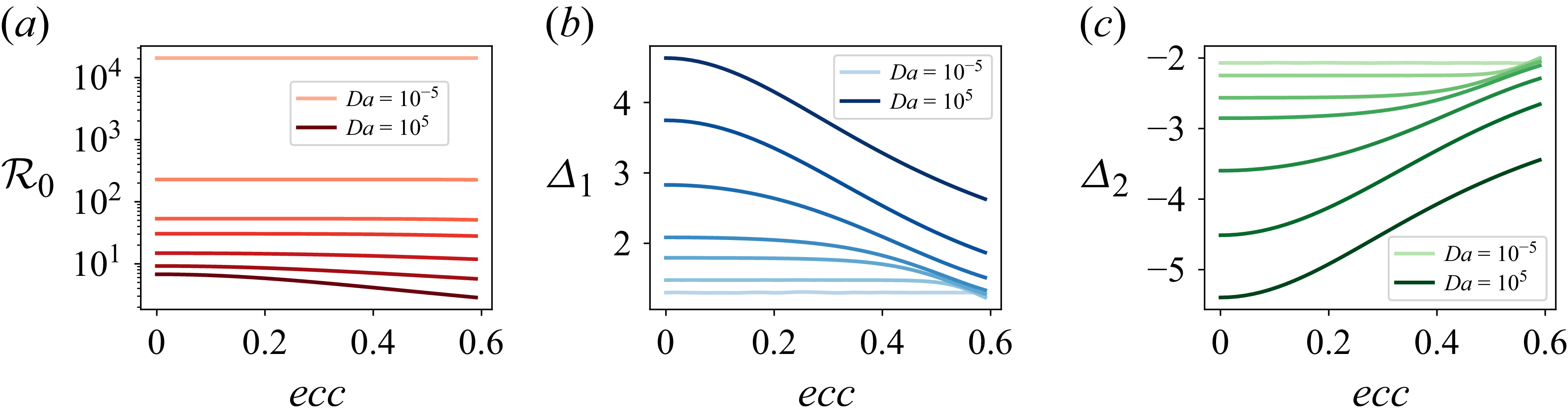
Figure 3 shows
 $\mathcal{R}_0$
,
 $\varDelta _1$
and
 $\varDelta _2$
as functions of the eccentricity,
 $ecc$
, for various Darcy numbers across a wide range,
 $ \textit{Da}\in [10^{-5},10^{5}]$
, to show all possible behaviours. First, from figure 3(a), we observe that the base resistance,
 $\mathcal{R}_0$
, decreases by orders of magnitude with increasing
 $ \textit{Da}$
, because the annular space is ‘less’ resistive (more ‘open’), and the viscous drag of the walls becomes dominant. Then,
 $\mathcal{R}_0$
decreases with
 $ecc$
because of the larger region away from the no-slip walls where the flow experiences less resistance (see figure 2(b)). Conversely, as
 $ \textit{Da}$
decreases, the viscous drag near the wall is confined to thin boundary layers (figure 2), and the flow profile is plug-like throughout the domain (Nield & Bejan Reference Nield and Bejan2017), leading
 $\mathcal{R}_0$
to become largely independent of
 $ecc$
for
 $ \textit{Da} \ll 1$
. This observation can also be rationalised via (2.3) and (2.4), noting that, for
 $ \textit{Da}\ll 1$
, the ‘outer solution’ is
 $\hat {V}_Z \sim Da$
and thus
 $\mathcal{R}_0 \sim 1/(Da\, A)$
, where
 $A$
is the area of the eccentric annular cross-section. For our problem, both boundaries are circles, and a standard exercise shows that
 $A = \pi (R_{e,0}^2 - 1) = 4.90$
is the dimensionless area of the annular space, which is independent of
 $ecc$
for our set-up (figure 1). Furthermore, using
 $\hat {V}_Z \sim Da$
and
 $\mathcal{R}_0 \sim 1/(Da\, A)$
for
 $ \textit{Da}\ll 1$
, it is easy to show that
 $\varDelta _1 \sim 2\pi R_a/A \approx 1.28$
and
 $\varDelta _2 \sim - 2\pi R_{e,0}/A \approx -2.05$
, independent of
 $ecc$
as
 $ \textit{Da}\to 0$
, precisely matching the small-
 $ \textit{Da}$
curves’ plateaus seen in figures 3(b) and 3(c), respectively.
Finally, from figures 3(b) and 3(c), we observe that
 $\varDelta _1$
(due to arterial wave displacement) and
 $\varDelta _2$
(due to endfeet-layer, i.e. outer-wall, displacement) exhibit similar trends with respect to
 $ecc$
and
 $ \textit{Da}$
when considering their magnitudes. However, while the arterial wave increases total resistance (
 $\varDelta _1\gt 0$
) due to conduit constriction, brain compliance decreases it (
 $\varDelta _2\lt 0$
) due to conduit expansion.
Computed dependence of the resistance perturbation expansion parameters,
 $\mathcal{R}_0$
,
 $\varDelta _1$
and
 $\varDelta _2$
from (2.6), on the eccentricity,
 $ecc$
, for selected values of the Darcy number,
 $ \textit{Da} = 10^{-5}, 10^{-3}, 5\times 10^{-3}, 10^{-2}, 3\times 10^{-2}, 10^{-1}$
and
 $10^5$
(light to dark curves).

2.4. The pressure
To derive the equation for axial pressure evolution that incorporates peristalsis at the inner wall and compliance at the outer wall of the fluidic domain, let us consider the dimensionless continuity equation. Integrating the dimensionless continuity equation over an arbitrary (potentially deformed) cross-section
 $\varOmega _{\textit{cs}}$
, the axial term yields
 $\partial Q/\partial Z$
(using the Leibniz rule and the no-slip BCs on the walls), while the transverse divergence becomes a boundary flux by Gauss’ theorem
 \begin{align} \frac {\partial Q}{\partial Z} + \oint _{\partial \varOmega _{\textit{cs}}} \boldsymbol{V}\boldsymbol{\cdot }\boldsymbol{n} \, \text{d}s = 0, \end{align}
where
 $\boldsymbol{n}$
is the outward normal to the fluid domain (i.e. it has opposite direction at the two walls) and
 $\text{d}s = r\,\text{d}\theta$
is an arclength element. Splitting up the line integral in (2.7) into two parts, we obtain
 \begin{align} \frac {\partial Q}{\partial Z} - \int _0^{2\pi } \boldsymbol{V}\boldsymbol{\cdot }\boldsymbol{n}|_a \, R_{a,c} \, \text{d}\theta + \int _0^{2\pi } \boldsymbol{V}\boldsymbol{\cdot }\boldsymbol{n}|_e \, R_e \, \text{d}\theta = 0. \end{align}
Now, we use the kinematic BCs (2.5) to evaluate the integrals and eliminate
 $Q$
via (2.4a
). A straightforward but lengthy calculation shows that (2.8) yields a nonlinear PDE for the pressure
 \begin{align} \underbrace {\frac {\partial }{\partial Z} \left (\frac {1}{\mathcal{R}} \frac {\partial P}{\partial Z} \right )}_{\textit{viscous resistance}} - \underbrace {2 \pi \left (1+\epsilon \mathcal{T} \right ) \mathcal{T}'}_{\textit{peristalsis}} - \underbrace {2\pi \left (R_{e,0} + \epsilon \beta P\right ) \beta \frac {\partial P}{\partial T}}_{w\textit{all compliance}} = 0. \end{align}
The equation can be solved using a relevant set of BCs on
 $P$
at
 $Z=0,L$
, including Dirichlet or resistance (Robin) ones. We focus on periodic BCs:
 $P(0,T)=P(L,T)$
for all
 $T\gt 0$
.
We focus on periodic cardiac pulsations with
 $\mathcal{T}(\boldsymbol{\cdot })=\sin (\boldsymbol{\cdot })$
. Let
 $P(Z,T)=\mathcal{P}(\varXi )$
be the pressure waveform in the moving frame
 $\varXi = Z-T$
. In this case, a perturbation solution,
 $\mathcal{P} = \mathcal{P}_0 + \epsilon \mathcal{P}_1 + \cdots$
in
 $\epsilon \ll 1$
, of (2.9) can be constructed. After a lengthy but straightforward exercise (see Appendix A), we find
 \begin{align} \mathcal{P}_0(\varXi ) = \frac {2\pi \mathcal{R}_0}{1+B^2} + \frac {2\pi \mathcal{R}_0}{\sqrt {1+B^2}} \sin (\varXi +\phi _P), \qquad \phi _P = -\tan ^{-1}(1/B), \end{align}
where we have introduced
 $B = 2 \pi \mathcal{R}_0 R_{e,0} \beta$
for convenience.
Simultaneously, we discretise (2.9) in time using the
 $\vartheta$
-scheme (see, e.g. Logg et al. Reference Logg, Mardal and Wells2012, Ch. 31) and in space using first-order Lagrange finite elements with a periodic domain constraint, as described in Appendix B.3. To shorten the transient to the periodic state, we used (2.10) to generate the initial condition
 $P(Z,0)$
. The results are reported as the mean of the last three cycles.
We verified our model’s self-consistency by simulating the case
 $ \textit{Da}\to \infty$
,
 $\beta =0$
and
 $ecc=0.2$
, and confirming exact agreement of
 $Q(L/4,T)$
and
 $P(L/4,T)$
with predictions from an independent numerical implementation of (4.2) and (4.4) of Coenen et al. (Reference Coenen, Zhang and Sánchez2021) for this same geometry. Additional details on verification and validation, as well as the rationale for the choices of the mesh element count, the number of time steps per cardiac cycle and the number of cardiac cycles, are provided in Appendix B.3.
3. Results and discussion
We now explore the implications of the outer wall’s compliance in a porous annular conduit of length
 $\ell =2\lambda$
(thus,
 $L=\kappa \ell =4\pi$
), consistent with the geometries considered by Carr et al. (Reference Carr, Thomas, Liu and Shang2021) and Coenen et al. (Reference Coenen, Zhang and Sánchez2021), and relative wave amplitude
 $\epsilon = 0.02$
(see table 1 for default parameters) by simulating (2.9) subject to periodic BCs. The long conduit, while not representative of the typical shorter, bifurcation-free perivascular segments, yields a finite net pumping rate due to peristalsis, which we aim to understand in this work.
3.1. Flow metrics for compliant conduits with different eccentricities
First, in figure 4, we examine the effect of artery eccentricity,
 $ecc$
, on the relevant flow metrics (resistance, pressure gradient and flow rate). We consider three Darcy numbers (
 $ \textit{Da}=10^{-3}$
,
 $10^{-2}$
and
 $10^{-1}$
), corresponding to the annular conduit transitioning from a porous to an open space. In the top row of figure 4, we observe that, for small
 $ \textit{Da}$
, the resistance
 $\mathcal{R}$
is high, as expected, due to the substantial obstruction posed by the porous medium, and vice versa for larger
 $ \textit{Da}$
. For
 $ \textit{Da}=10^{-3}$
, the resistance curves nearly overlap for all
 $ecc$
values because the flow is dominated by the porous drag, and hence becomes independent of
 $ecc$
(recall figure 3). On the other hand, for the less porous spaces (
 $ \textit{Da}=10^{-2}$
and
 $10^{-1}$
), resistance decreases with increasing eccentricity, and the curves are distinct.
Second, we examine the pressure gradient
 $-\partial P/\partial Z$
and the flow rate
 $Q$
in the bottom row of figure 4. The pressure gradient is largely independent of
 $ \textit{Da}$
and
 $ecc$
because, for periodic BCs, it is driven by the peristaltic wave (the only forcing). Meanwhile, the resistance adjusts to the flow conditions, and the flow rate reflects it. Specifically, the
 $Q$
amplitude increases with
 $ \textit{Da}$
, as the space becomes more open. Likewise, the
 $Q$
amplitude increases with
 $ecc$
due to the emergence of a low-resistance channel away from the outer wall (recall figure 2(b)).
Effect of eccentricity on the flow metrics for (a)
 $ \textit{Da}=10^{-3}$
(note that all curves overlap), (b)
 $ \textit{Da}=10^{-2}$
and (c)
 $ \textit{Da}=10^{-1}$
. Each column corresponds to a Darcy number, while the rows represent flow metrics, with resistance in the top row, and the pressure gradient and flow rate in the bottom row. All plots are at
 $Z=L/4$
and
 $\beta =10$
.

3.2. Compliance of the outer wall and flow–pressure phasing
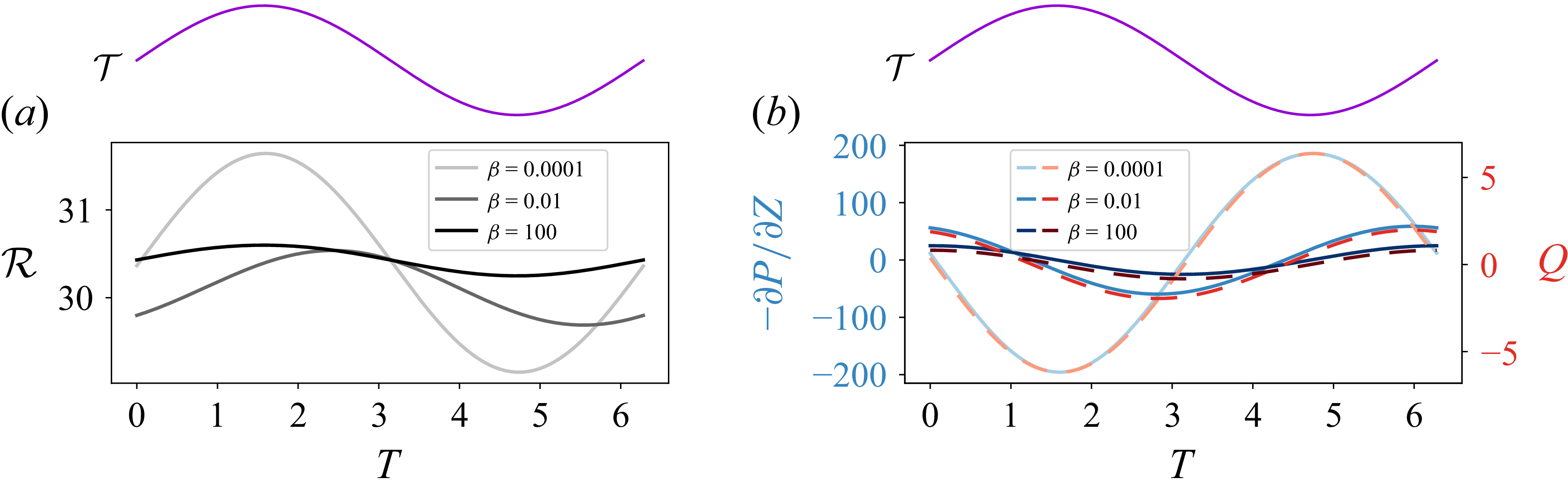
Next, we study the effect of compliance across these scenarios by varying the compliance number in figure 5. Recall that, since
 $\beta = \mathcal{C} \mu \omega /(\kappa ^2 r_0^3)$
, the overall effect of compliance is not solely controlled by the elasticity-related constant
 $\mathcal{C}$
but also by the artery radius
 $r_0$
, fluid viscosity
 $\mu$
, wave frequency
 $\omega$
and wavenumber
 $\kappa$
. In this figure, we only consider
 $ \textit{Da}=10^{-2}$
; the trends are similar for other choices of
 $ \textit{Da}$
. A smaller
 $\beta$
(stiffer outer wall) leads to higher amplitude of the resistance, pressure gradient and flow rate, and vice versa. For a more compliant PAS, the outer wall expands in response to the hydrodynamic forces within, increasing the local cross-sectional area and reducing the amplitude of hydraulic resistance. The higher compliance also attenuates the pressure gradient amplitude by redistributing the driving energy into wall deformation. Consequently, the instantaneous flow rate amplitudes decrease with
 $\beta$
.
Effect of compliance on flow metrics. Time series of (a) resistance
 $\mathcal{R}$
, (b) pressure gradient
 $-\partial P/\partial Z$
and flow rate
 $Q$
. The driving peristaltic wave profile,
 $\mathcal{T}$
, is shown above each plot. In (b), the
 $-\partial P/\partial Z$
and
 $Q$
curves corresponding to
 $\beta =100$
are multiplied by a factor of 4000 to highlight the phase relationship. All curves are for
 $ \textit{Da}=10^{-2}$
,
 $ecc=0.2$
and
 $Z=L/4$
.

In passing, we note that
 $\beta = 100$
means that
 $\epsilon \beta = 2 \not\kern-1pt \ll 1$
, yet this highly compliant case does not invalidate the domain-perturbation expansion introduced in (2.6) above because the actual approximation made can be rephrased as
 $\max |\epsilon \beta P| \ll R_{e,0}$
. Upon using
 $P\simeq \mathcal{P}_0$
and (2.10), we calculate
 \begin{align} \max |\epsilon \beta P| \simeq \frac {\epsilon }{R_{e,0}} \max _B \frac {B(1+\sqrt {1+B^2})}{1+B^2} = \frac {3\sqrt {3} \epsilon }{4R_{e,0}} \approx 0.016 \ll 1.6 = R_{e,0}. \end{align}
This a posteriori check highlights that the wall displacement saturates: a more compliant wall deforms more readily but is loaded by a correspondingly smaller pressure.
The most prominent feature in figure 5 is the phase shift of
 $-\partial P/\partial Z$
and
 $Q$
(relative to the driving peristaltic wave
 $\mathcal{T}$
), which is a strong function of
 $\beta$
. The phase is evident from (2.10). Specifically, we find that the phase of the pressure relative to the driving wave is
 $\phi _{P}$
given in (2.10b
), with the pressure gradient shifted by a further quarter period,
 $\phi _{-\partial P/\partial Z} = \phi _P - \pi /2$
(see Appendix A.3). For even moderate
 $\beta$
, the phase saturates to
 $\phi _{-\partial P/\partial Z} \to - \pi /2$
rapidly since
 $\mathcal{R}_0$
is large; in the opposite limit
 $\phi _{-\partial P/\partial Z} \to -\pi$
as
 $\beta \to 0$
. Both of these limits are evident in figure 5(b), keeping in mind that a positive phase in
 $\varXi$
appears as a lag when plotting against
 $T$
at fixed
 $Z$
because
 $\varXi = Z - T$
, and vice versa. Although previous work has noted that phase differences between the peristaltic wave, flow, pressure and deformation can affect net glymphatic transport in brain tissue (Li et al. Reference Li, Dabiri and Ardekani2025; Nozaleda et al. Reference Nozaleda, Coenen, Haughton and Sánchez2025), no analytical connection was made to brain tissue compliance. Our model precisely quantifies this phase in terms of the key dimensionless parameters, specifically the compliance number.
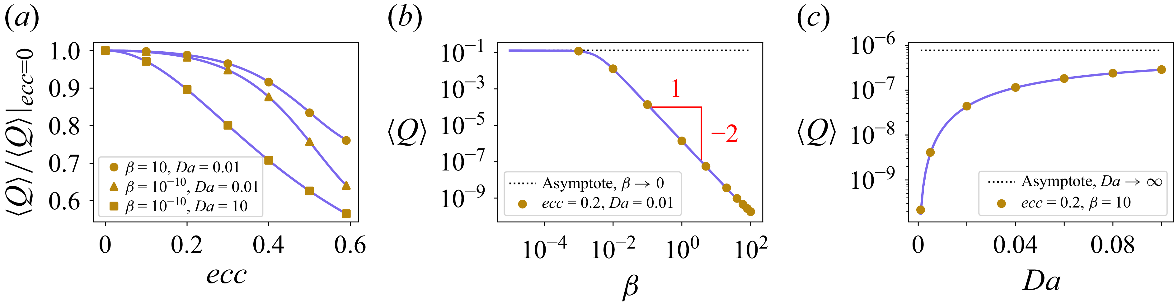
Pumping (space–time or cycle-averaged) flow rate as a function of (a) eccentricity,
 $ecc$
, (b) compliance,
 $\beta$
, and (c) Darcy number,
 $ \textit{Da}$
. The darker (purple) curves are based on the analytical approximation (3.2) for
 $\epsilon \ll 1$
. Cases with
 $\beta = 10^{-10}$
represent the rigid limit evaluated through the present compliant model.

3.3. Net pumping rate
Finally, we discuss the net pumping (cycle-averaged) flow rate
 $\langle Q \rangle$
. Figure 6(a) shows that
 $\langle Q \rangle$
decreases with
 $ecc$
, even for
 $ \textit{Da}\lt \infty$
and
 $\beta \gt 0$
. The case of
 $ \textit{Da}=10$
and
 $\beta =10^{-10}$
is illustrative of the rigid open channel of Coenen et al. (Reference Coenen, Zhang and Sánchez2021). Meanwhile, our model can handle a wide range of
 $ \textit{Da}$
and
 $\beta$
, as highlighted by the other two curves (
 $ \textit{Da}=0.01$
and
 $\beta =10^{-10}$
for a porous rigid channel, and
 $ \textit{Da}=0.01$
and
 $\beta =10$
for a porous compliant channel).
Figure 6(b) shows a new prediction of our model, namely that the net pumping is a strong function of compliance, decaying rapidly from the ‘ceiling’ value (achieved at
 $\beta =0$
and
 $ecc=0$
for a given
 $ \textit{Da}$
). A straightforward (but lengthy) perturbation calculation for
 $\epsilon \ll 1$
based on (2.9) (see Appendix A) yields an analytical result
 \begin{align} \langle Q \rangle = \frac {\pi \epsilon \varDelta _1}{1 + (2 \pi \mathcal{R}_0 R_{e,0}\beta )^2}, \end{align}
which rationalises the observations of figure 6(b). Two aspects of the result (3.2) are worth further interpretation. First, the compliance number always appears in the combination
 $B = 2\pi \mathcal{R}_0R_{e,0}\beta$
, so that the onset of the decay of
 $\langle Q \rangle$
is governed by the compliance number scaled by the base hydraulic resistance, and not by
 $\beta$
itself. Since
 $\mathcal{R}_0$
is large in a porous conduit (ranging from
 ${\approx} 30$
at
 $ \textit{Da} = 10^{-2}$
to
 ${\approx} 230$
at
 $ \textit{Da} = 10^{-3}$
in figure 3(a) at
 $ecc=0.2$
) and
 $R_{e,0} = 1.6$
, the ‘cross-over’ value
 $\beta ^*$
is such that
 $1 \approx (2 \pi \mathcal{R}_0 R_{e,0}\beta ^*)^2$
or
 $\beta ^* \approx 3\times 10^{-3}$
(
 $Da = 10^{-2}$
) and
 $4\times 10^{-4}$
(
 $Da = 10^{-3}$
). These compliance values are much smaller than the physiological range of table 1, implying that a penetrating PAS might always be in the
 $\beta ^{-2}$
tail of (3.2). In other words, even a very weakly compliant endfeet layer, which one might reasonably idealise as rigid, already suppresses the net pumping by orders of magnitude relative to the rigid-wall case. Second,
 $\mathcal{R}_0$
and
 $\varDelta _1$
themselves depend on
 $ecc$
and
 $ \textit{Da}$
in a non-trivial manner (recall § 2), so the cross-over
 $\beta$
value changes with the geometry and the porosity.
Finally, figure 6(c) shows that net pumping rapidly increases with
 $ \textit{Da}$
, meaning that porous spaces strongly inhibit net pumping compared with open ones. Specifically, from our analytical approximation, we find that
 $\langle Q \rangle \sim \epsilon Da^2 A/(2 R_{e,0}^2 \beta ^2)$
for
 $ \textit{Da} \ll 1$
from (3.2), since
 $\mathcal{R}_0 \sim 1/Da$
and
 $\varDelta _1 \sim 2\pi R_a/A$
as
 $ \textit{Da} \to 0$
.
4. Conclusion
Inspired by the mechanics of CSF flow in the PAS, we developed a two-way-coupled fluid–structure interaction model for peristaltically driven flow in an eccentric annular porous conduit with a compliant outer wall. The slenderness of the conduit allows the use of a long-wave (lubrication) approximation, reducing the problem to an unsteady PDE for the pressure (after pre-solving an equation for cross-sectional velocity). We calculated changes in hydraulic resistance due to peristalsis (arterial displacements) and deformation of the surrounding brain tissue using a perturbation expansion in the peristaltic wave amplitude.
The resulting computationally (and analytically) tractable model for flow in non-axisymmetric spaces with a compliant outer wall in hand allowed us to perform parameter-space studies, focusing on the effect of the eccentricity of space, the Darcy number (quantifying the porous drag within the space) and the compliance number (elasticity of the space’s outer confining wall) on the hydraulic resistance, the pressure gradient and the flow rate. In contrast to previous studies on rigid conduits (Carr et al. Reference Carr, Thomas, Liu and Shang2021; Coenen et al. Reference Coenen, Zhang and Sánchez2021), we discovered that compliance strongly reduces the net pumping rate, consistent with the simulations of Gan et al. (Reference Gan, Holstein-Rønsbo, Nedergaard, Boster, Thomas and Kelley2023). Analytical approximations of our reduced model under periodic BCs revealed a simple formula showing that the net pumping rate decays as the inverse square of the compliance number. Crucially, the onset of this decay is set by the compliance number scaled by the base resistance, which is large in a porous space; consequently, pumping is strongly reduced even for walls that are only weakly compliant. Similarly, we found that net pumping decreases in more obstructed spaces (i.e. at smaller Darcy numbers).
A future direction could be to consider other BCs, such as upstream and downstream resistance BCs, which are typically encountered when modelling a finite PAS segment. We could also extend the model to account for a porous outer wall (Gan et al. Reference Gan, Holstein-Rønsbo, Nedergaard, Boster, Thomas and Kelley2023; Takagi et al. Reference Takagi, Balmforth and Llewellyn Smith2024), which would require updating the BC at the outer wall and incorporating the transverse variation of pressure and velocity at
 $O((\kappa r_0)^2)$
(Coenen et al. Reference Coenen, Zhang and Sánchez2021). The transverse pressure variations could result in non-uniform deformation of the PAS outer wall for non-zero eccentricities. Other driving mechanisms of flow in the PAS can be considered, such as functional hyperaemia, which has a non-zero mean wave profile, unlike the sinusoidal wave profile used in our analysis. Finally, when the Womersley number is not small, it would be relevant to understand how elastoinertial rectification (Zhang & Rallabandi Reference Zhang and Rallabandi2024) contributes to the net pumping in non-axisymmetric geometries. It will also be relevant to analyse the role of the complex rheology of biofluids (Covarrubias et al. Reference Covarrubias, Bautista, Arcos and Méndez2026) in non-axisymmetric geometries.
Acknowledgements
Simulations were performed using the community clusters of the Rosen Center for Advanced Computing at Purdue University. We thank J.A. Gil Duque for helpful explorations of the model in its earlier stages.
Funding
This research was supported by the National Aeronautics and Space Administration (NASA) under FINESST Research Grant No. 80NSSC25K7350.
Declaration of interests
The authors report no conflict of interest.
Author contributions
N.S.: conceptualisation, formal analysis, data curation, software, validation, investigation, visualisation, methodology, writing – original draft, writing – review and editing, funding acquisition. I.C.C.: conceptualisation, formal analysis, supervision, validation, investigation, methodology, writing – original draft, writing – review and editing, project administration, funding acquisition.
Data availability statement
The scripts to reproduce the data that support the findings of this study are openly available in the Purdue University Research Repository (PURR) at http://doi.org/10.4231/NJ7B-5N87.
Appendix A. Detailed derivation of the analytical approximation(s) for
 $\epsilon \ll 1$

A.1 Transformation to a moving frame
Introducing the travelling wave pressure form
 $\mathcal{P}(\varXi = Z-T) = P(Z,T)$
so that
 $\partial P/\partial T = -\mathcal{P}'$
,
 $\partial P/\partial Z = +\mathcal{P}'$
, and
 $(\,\boldsymbol{\cdot }\,)' = d/\text{d}\varXi$
, we transform (2.9) into
 \begin{align} \left ( \frac {1}{\mathcal{R}} \mathcal{P}' \right )' - 2 \pi (1 + \epsilon \mathcal{T}) \mathcal{T}' + 2\pi \left ( R_{e,0} + \epsilon \beta \mathcal{P} \right ) \beta \mathcal{P}' = 0. \end{align}
To obtain the pumping rate, we integrate (A1) with respect to
 $\varXi$
 \begin{align} \frac {1}{\mathcal{R}} \mathcal{P}' - 2 \pi \big ( \mathcal{T} + \epsilon \mathcal{T}^2/2 \big ) + \beta \big ( 2\pi R_{e,0} \mathcal{P} + 2\pi \epsilon \beta \mathcal{P}^2/2 \big ) + C_\lambda = 0, \end{align}
where
 $C_\lambda$
is determined by the constraint that
 $\langle \mathcal{P}'\rangle \equiv \delta P_\lambda /(2\pi )$
, which represents some (arbitrary) pressure change per wavelength. To impose this constraint, we multiply (A2) by
 $\mathcal{R}$
and average over a cycle, i.e. we apply
 $\langle \, \boldsymbol{\cdot }\, \rangle = ({1}/{2\pi }) \int _0^{2\pi } ( \, \boldsymbol{\cdot }\, ) \, \text{d}\varXi$
, to find
 \begin{align} C_\lambda = \frac {2 \pi \big ( \langle \mathcal{T}\mathcal{R}\rangle + \epsilon \langle \mathcal{T}^2\mathcal{R}\rangle /2 \big ) - \beta \big ( 2\pi R_{e,0} \langle \mathcal{P} \mathcal{R}\rangle + 2\pi \epsilon \beta \langle \mathcal{P}^2\mathcal{R}\rangle /2 \big ) - \delta P_\lambda /(2\pi )}{\langle \mathcal{R} \rangle }. \end{align}
Now, returning to (A2) and recognising that the first term on the left-hand side is
 $-Q$
, we once again average and solve for
 \begin{align} \langle Q \rangle = C_\lambda - 2\pi \big (\langle \mathcal{T} \rangle - \beta R_{e,0}\langle \mathcal{P} \rangle \big ) - \pi \epsilon \big ( \langle \mathcal{T}^2 \rangle - \beta ^2 \langle \mathcal{P}^2 \rangle \big ) . \end{align}
Note that this result is not closed; both
 $\mathcal{R}$
and
 $\mathcal{P}$
still need to be computed consistently from the coupled fluid–structure interaction problem. To overcome this difficulty and obtain some analytical insight, we proceed by a perturbation expansion in
 $\epsilon \ll 1$
.
A.2 Leading-order pressure solution in the moving frame
Performing a perturbation expansion
 $\mathcal{P} = \mathcal{P}_0 + \epsilon \mathcal{P}_1 + O(\epsilon ^2)$
, consistent with the perturbation expansion for
 $\mathcal{R}$
in (2.6), and substituting it into (A1), we obtain a linear ordinary differential equation for
 $\mathcal{P}_0$
 \begin{align} \frac {1}{\mathcal{R}_0} \mathcal{P}_0'' - 2 \pi \mathcal{T}' + 2\pi R_{e,0} \beta \mathcal{P}_0' = 0. \end{align}
This equation captures the leading-order contributions of both peristalsis and compliance.
Multiplying (A5) by
 $\mathcal{R}_0$
and integrating once, we have
 \begin{align} \mathcal{P}_0' - 2 \pi \mathcal{R}_0 \mathcal{T} + B \mathcal{P}_0 = B C_1, \qquad B = 2 \pi \mathcal{R}_0 R_{e,0} \beta . \end{align}
Using the integrating factor
 $\text{e}^{B\varXi }$
, we can solve the latter
 \begin{align} \mathcal{P}_0(\varXi ) = 2 \pi \mathcal{R}_0 \text{e}^{-B\varXi } \int \mathcal{T}(\hat{\varXi} ) \text{e}^{B\hat {\varXi }} \, \text{d}\hat {\varXi } + C_1 + C_2 \text{e}^{-B\varXi }. \end{align}
Thus, we have obtained leading-order analytical solution
 $\mathcal{P}_0$
, for the pressure variation, in terms of the base resistance
 $\mathcal{R}_0$
, the compliance number
 $\beta$
and the average outer radius
 $R_{e,0}$
, for a given peristaltic waveform
 $\mathcal{T}$
. For
 $\mathcal{T}(\varXi ) = \sin (\varXi )$
, (A7) yields
 \begin{align} \mathcal{P}_0(\varXi ) = 2 \pi \mathcal{R}_0 \left ( \frac {B \sin \varXi - \cos \varXi }{1 + B^2} \right ) + C_1 + \; C_2 \text{e}^{-B\varXi }. \end{align}
A.3 Periodic BCs
For periodic BCs, we enforce
 $\mathcal{P}(0) = \mathcal{P}(2\pi )$
on the solution from (A8), to obtain
 \begin{align} C_2 = 0,\qquad C_1 = \text{arbitrary}. \end{align}
Without loss of generality,
 $C_1$
is chosen by requiring that
 $\mathcal{P}_0(0)=0$
, thus
 \begin{align} \mathcal{P}_0(\varXi ) = 2 \pi \mathcal{R}_0 \left ( \frac {1 - \cos \varXi + B \sin \varXi }{1 + B^2} \right )\!. \end{align}
We verify in Appendix A.4 that the net pumping rate is independent of the choice
 $\mathcal{P}_0(0)=0$
.
Equivalently, in amplitude–phase form, (A10) becomes
 \begin{align} \mathcal{P}_0(\varXi ) = \frac {2\pi \mathcal{R}_0}{1+B^2} + \frac {2\pi \mathcal{R}_0}{\sqrt {1+B^2}} \sin (\varXi +\phi _P), \qquad \phi _P = -\tan ^{-1}(1/B), \end{align}
taking the principal branch of
 $\tan ^{-1}$
since
 $\cos \phi _P = B/\sqrt {1+B^2}\ge 0$
and
 $\sin \phi _P = -1/\sqrt {1+B^2}\lt 0$
; thus,
 $\phi _P\in [-\pi /2,0)$
. Differentiating (A11), and using
 $-\cos \xi = \sin (\xi - \pi /2)$
 \begin{align} -\frac {\partial P}{\partial Z} = -\mathcal{P}_0' = \frac {2\pi \mathcal{R}_0}{\sqrt {1+B^2}}\,\sin \!\left (\varXi +\phi _P-{\pi }/{2}\right ), \end{align}
so that
 $\phi _{-\partial P/\partial Z} = \phi _P - \pi /2$
, with
 $\phi _{-\partial P/\partial Z}\to -\pi$
as
 $\beta \to 0$
and
 $\to -\pi /2$
as
 $\beta \to \infty$
. The rigid limit provides a sanity check: setting
 $B=0$
in (A10) gives
 $-\partial P/\partial Z = -2\pi \mathcal{R}_0\sin \varXi$
(anti-phase with the peristaltic wave).
A.4 Pumping rate
To proceed, we continue with the
 $\epsilon \ll 1$
perturbation expansion by substituting (2.6) into (A4), having eliminated
 $C_\lambda$
using (A3), to obtain
 \begin{align} \langle Q \rangle = &\left [2 \pi \Big ( \langle \mathcal{T}{\mathcal{R}_0}\rangle + \epsilon \varDelta _1 \langle \mathcal{T}^2 {\mathcal{R}_0}\rangle + \epsilon \beta \varDelta _2 \langle \mathcal{T}\mathcal{P}{\mathcal{R}_0}\rangle + \epsilon \langle \mathcal{T}^2{\mathcal{R}_0}\rangle /2 \Big ) + O(\epsilon ^2) \right ]\nonumber \\& \times \frac {1}{\langle {\mathcal{R}_0} \rangle } \left [1-\epsilon \big (\varDelta _1\langle \mathcal{T} \rangle +\varDelta _2\beta \langle \mathcal{P}\rangle \big ) + O(\epsilon ^2) \right ]\nonumber \\& - \left [\beta \Big ( 2\pi R_{e,0} \langle \mathcal{P} {\mathcal{R}_0}\rangle + 2\pi R_{e,0} \epsilon \varDelta _1 \langle \mathcal{P}\mathcal{T} {\mathcal{R}_0}\rangle + 2\pi R_{e,0} \epsilon \beta \varDelta _2 \langle \mathcal{P}^2{\mathcal{R}_0}\rangle \Big.\right. \nonumber \\& \qquad \Big.\left. + 2\pi \epsilon \beta \langle \mathcal{P}^2{\mathcal{R}_0}\rangle /2 + O(\epsilon ^2) \Big )\right ]\nonumber \\& \times \frac {1}{\langle {\mathcal{R}_0} \rangle } \left [1-\epsilon \big (\varDelta _1\langle \mathcal{T} \rangle +\varDelta _2\beta \langle \mathcal{P}\rangle \big ) + O(\epsilon ^2) \right ]\nonumber \\& -\pi \epsilon \Big ( \langle \mathcal{T}^2 \rangle -\beta ^2 \langle \mathcal{P}^2 \rangle \Big ) - 2\pi \Big (\langle \mathcal{T} \rangle - \beta R_{e,0}\langle \mathcal{P} \rangle \Big ) + O(\epsilon ^2). \end{align}
Note that
 $\mathcal{R}_0$
is independent of
 $\varXi$
, thus
 $\langle \mathcal{R}_0\rangle = \mathcal{R}_0$
and this term was factored out and cancelled. We have also carried along the contribution from the Taylor series expansions of the denominators. Regrouping terms, we find many self-cancel and
 $\langle \mathcal{T}\rangle =0$
, due to the periodicity of the peristaltic wave, removes several others. Substituting the perturbation expansion for
 $\mathcal{P}$
, we obtain
 \begin{align} \langle Q \rangle = 2 \pi \epsilon \big [ \varDelta _1 \langle \mathcal{T}^2\rangle + \beta ( \varDelta _2 - R_{e,0} \varDelta _1 )\langle \mathcal{T}\mathcal{P}_0\rangle - \beta ^2 R_{e,0} \varDelta _2 \big ( \langle \mathcal{P}_0^2\rangle - \langle \mathcal{P}_0\rangle ^2 \big ) \big ] + O(\epsilon ^2) . \end{align}
We observe that compliance introduces two new terms: one proportional to the cross-correlation between the peristaltic and pressure waveforms, and the other proportional to the variance of the pressure waveform. Setting
 $\beta =0$
, we recover (4.5) of Coenen et al. (Reference Coenen, Zhang and Sánchez2021).
Note that setting
 $\mathcal{P}_0(0)=0$
leads to
 $\langle \mathcal{P}_0\rangle \ne 0$
. While the physical gauge is fixed by the reference pressure
 $p_{\textit{ref}}$
in § 2, fixing
 $\mathcal{P}_0(0)=0$
means that the solution (A10) corresponds to placing the pressure reference at
 $\varXi = 0$
. Importantly, two features of the problem render our results insensitive to the arbitrary choice
 $\mathcal{P}_0(0)=0$
. First, the leading-order equation, (A5), involves
 $\mathcal{R}_0$
only, hence
 $\mathcal{P}_0$
is only determined up to the additive constant,
 $C_1$
. Second, and more importantly, the net pumping rate in (A14) is invariant under
 $\mathcal{P}_0 \mapsto \mathcal{P}_0 + C_1$
because, even though
 $\langle \mathcal{T}\mathcal{P}_0\rangle \mapsto \langle \mathcal{T}\mathcal{P}_0\rangle + C_1 \langle \mathcal{T}\rangle$
,
 $C_1 \langle \mathcal{T}\rangle = 0$
by periodicity of the peristaltic wave. Meanwhile the term
 $\langle \mathcal{P}_0^2\rangle - \langle \mathcal{P}_0\rangle ^2$
in (A14) being a variance is unaffected by constant shifts.
Finally,
 $\langle \mathcal{P}_0\rangle ^2$
,
 $\langle \mathcal{P}_0^2\rangle$
and
 $\langle \mathcal{T} \mathcal{P}_0 \rangle$
in (A14) are evaluated based on the leading-order solution (A8) with
 $C_2=0$
,
 $C_1 = 2\pi \mathcal{R}_0/(1+B^2)$
and
 $\mathcal{T}(\varXi ) = \sin (\varXi )$
. Specifically, we compute
 \begin{align} \langle \mathcal{P}_0 \rangle ^2 &= \left [\frac {1}{2\pi } \int _0^{2\pi } \mathcal{P}_0( \varXi ) \, \text{d}\varXi \right ]^2 = 4 \pi ^{2} \mathcal{R}_{0}^{2} \frac {1}{(1 + B^{2})^{2}}, \\[-10pt] \nonumber \end{align}
 \begin{align} \langle \mathcal{P}_0^2 \rangle &= \frac {1}{2\pi } \int _0^{2\pi } \big [\mathcal{P}_0( \varXi )\big ]^2 \, \text{d}\varXi = 2\pi ^2 \mathcal{R}_0^2 \frac {3 + B^2}{(1 + B^2)^2}, \\[-10pt] \nonumber \end{align}
 \begin{align} \langle \mathcal{T} \mathcal{P}_0 \rangle &= \frac {1}{2\pi } \int _0^{2\pi } \mathcal{T}(\varXi )\mathcal{P}_0( \varXi ) \, \text{d}\varXi = \pi \mathcal{R}_0 \frac {B}{1 + B^2}. \\[10pt] \nonumber \end{align}
Using (A15) in (A14), we can evaluate the net pumping rate
 $\langle Q \rangle$
for
 $\epsilon \ll 1$
 \begin{align} \langle Q \rangle = \frac {\pi \epsilon \varDelta _1}{1 + B^2} \sim \begin{cases} \pi \epsilon \varDelta _1, &\quad \beta \to 0,\\[6pt]\pi \epsilon \varDelta _1 \left ( \frac {1}{4 \pi ^2 \mathcal{R}_0^2 R_{e,0}^2} \right ) \beta ^{-2}, &\quad \beta \to \infty . \end{cases} \end{align}
Appendix B. FEM simulation details: weak forms, verification and validation
B.1 The axial momentum equation
B.1.1 Weak form
The axial momentum equation (2.3) can be written in a weak (variational) form by standard steps (Logg et al. Reference Logg, Mardal and Wells2012; Alnaes et al. Reference Alnaes, Blechta, Hake, Johansson, Kehlet, Logg, Richardson, Ring, Rognes and Wells2015). The variational problem to be solved is then: find
 $\hat {V}_Z$
such that, for every
 $\varPsi$
,
 $a(\hat {V}_Z,\varPsi )=l(\varPsi )$
, where the bilinear and linear forms are, respectively,
 \begin{align} a(\hat {V}_Z,\varPsi ) &= \int _{\varOmega _{\textit{cs}}} \left [\boldsymbol{\nabla }\hat {V}_Z \boldsymbol{\cdot }\boldsymbol{\nabla }\varPsi + \frac {1}{Da} \hat {V}_Z \varPsi \right ] \text{d}A, \\[-12pt] \nonumber \end{align}
 \begin{align} l(\varPsi ) &= \int _{\varOmega _{\textit{cs}}} \varPsi \, \text{d}A. \\[10pt] \nonumber \end{align}
Here,
 $\varPsi$
is a ‘test’ function from a first-order Lagrange finite element space (Logg et al. Reference Logg, Mardal and Wells2012). As before,
 $\varOmega _{\textit{cs}}$
is the domain representing the cross-section of the conduit, and
 $\text{d}A$
is the area element. The no-slip BC
 $\hat {V}_Z = 0$
on
 $\partial \varOmega _{\textit{cs}}$
was strongly imposed using the FEniCS’ built-in DirichletBC, eliminating those degrees of freedom from the subsequent matrix problem.
The two-dimensional computational geometry of the eccentric annular cross-section was constructed and meshed using the mesh-generation tool mshr. Then, the solution (B1) is obtained using the solve function in FEniCS with its default settings, which internally calls LinearVariationalSolver.
B.1.2 Verification and validation
We performed a verification of the axial momentum equation’s solution by computing the relative errors for the velocity field and hydraulic resistance values for meshes with
 $216\,532$
,
 $863\,743$
and
 $3\,459\,071$
elements (corresponding to mshr refinement level parameters of
 $300$
,
 $600$
and
 $1200$
, respectively at
 $ecc=0.2$
). The verification was performed for the geometry with
 $ecc=0.2$
and
 $ \textit{Da}=10^{-5}$
. The velocity
 $L^2$
error decreased from
 $2.17\,\%$
at
 $216\,532$
elements to
 $0.60\,\%$
at
 $863\,743$
elements, relative to the fine-mesh reference solution, which translates to a corresponding decrease in resistance error from
 $0.19\,\%$
to
 $0.04\,\%$
over the same mesh refinement. This monotonic decrease in both error metrics with increasing mesh resolution confirms convergence of the numerical solution, and the small resistance error (under
 $0.2\,\%$
even at the coarsest mesh) indicates that the mesh with
 $863\,743$
elements (refinement level
 $600$
) provides sufficient accuracy for resistance calculations in this geometry.
To validate the numerical implementation, we compared the finite element solution against an analytical solution available for the concentric annulus case
 $(ecc = 0)$
. In this case, since the domain is an axisymmetric annulus, the analytical solution of the boundary-value problem (2.3) is easily found in terms of modified Bessel functions of the first and second kinds (
 $\mathrm{I}_0$
and
 $\mathrm{K}_0$
)
 \begin{align} \hat {V}_Z(R) = Da - \frac {Da\left [\mathrm{K}_0\!\left (\dfrac {R_e}{\sqrt {Da}}\right ) - \mathrm{K}_0\!\left (\dfrac {R_a}{\sqrt {Da}}\right )\right ]} {\mathrm{I}_0\!\left (\dfrac {R_a}{\sqrt {Da}}\right )\mathrm{K}_0\!\left (\dfrac {R_e}{\sqrt {Da}}\right ) - \mathrm{I}_0\!\left (\dfrac {R_e}{\sqrt {Da}}\right )\mathrm{K}_0\!\left (\dfrac {R_a}{\sqrt {Da}}\right )}\, \mathrm{I}_0\!\left (\frac {R}{\sqrt {Da}}\right )\nonumber \\[5pt]- \frac {Da\left [\mathrm{I}_0\!\left (\dfrac {R_a}{\sqrt {Da}}\right ) - \mathrm{I}_0\!\left (\dfrac {R_e}{\sqrt {Da}}\right )\right ]} {\mathrm{I}_0\!\left (\dfrac {R_a}{\sqrt {Da}}\right )\mathrm{K}_0\!\left (\dfrac {R_e}{\sqrt {Da}}\right ) - \mathrm{I}_0\!\left (\dfrac {R_e}{\sqrt {Da}}\right )\mathrm{K}_0\!\left (\dfrac {R_a}{\sqrt {Da}}\right )}\, \mathrm{K}_0\!\left (\frac {R}{\sqrt {Da}}\right ). \end{align}
The numerical solution on the default grid was compared with the analytical profile (B2) for the same concentric (axisymmetric) annular geometry and
 $ \textit{Da}=10^{-5}$
(a ‘worst case scenario’ to ensure proper resolution of the boundary layer near the outer wall for
 $ \textit{Da} \ll 1$
). We computed the relative
 $L^2$
error
 \begin{align} \varepsilon _{L^2} = \frac {\big \lVert \hat {V}_{Z,\textit{analytical}} - \hat {V}_{Z,\textit{numerical}} \big \rVert _{L^2(\varOmega _{\textit{cs}})}}{\big \lVert \hat {V}_{Z,\textit{analytical}} \big \rVert _{L^2(\varOmega _{\textit{cs}})}} \end{align}
over the full two-dimensional annular domain
 $\varOmega _{\textit{cs}}$
using built-in FEniCS functions. For the mesh with
 $864\,834$
elements (corresponding to refinement level
 $600$
at
 $ecc=0$
; note that the unstructured mesh generation leads to slightly different element counts for different
 $ecc$
values), the relative
 $L^2$
error was
 $0.7\,\%$
, indicating strong agreement between the numerical and analytical solutions.
B.2 Resistance contributions
The derivatives in (2.6) were calculated by finite differences, using the information post-processed from the
 $\hat {V}_Z$
solution. Specifically, a central-difference scheme was used as follows:
 \begin{align} \varDelta _1 &= \left [\frac {1}{\mathcal{R}}\frac {\partial \mathcal{R}}{\partial R_a}\right ]_0 = \frac {1}{\mathcal{R}_0} \left [\frac {\mathcal{R}|_{R_a = 1+h}-\mathcal{R}|_{R_a=1-h}}{2h}\right ]_{\textit{fixed $R_e$}}, \\[-12pt] \nonumber \end{align}
 \begin{align} \varDelta _{2} &= \left [\frac {1}{\mathcal{R}}\frac {\partial \mathcal{R}}{\partial R_e}\right ]_0 = \frac {1}{\mathcal{R}_0} \left [\frac {\mathcal{R}|_{R_e=R_{e,0}+h}-\mathcal{R}|_{R_e=R_{e,0}-h}}{2h}\right ]_{\textit{fixed $R_a$}}. \\[10pt] \nonumber \end{align}
Note that these derivatives are evaluated at fixed axes offset
 $d$
, and therefore at fixed
 $ecc$
by construction.
In the FEniCS code, we calculated the resistances appearing in (B4) by perturbing the boundary and regenerating the mesh, with either the inner or outer circle fixed (as denoted). Then, we evaluated
 $\mathcal{R}$
according to (2.4b
) on the new geometry. We limited the eccentricity to
 $ecc \leq 0.59$
to avoid the degenerate/tangent case (here,
 $ecc = 0.6$
), for which evaluating
 $\mathcal{R}|_{R_a = 1+h}$
or
 $\mathcal{R}|_{R_e = R_{e,0} - h}$
in (B4) is not possible due to the intersection of the circles.
Next, we performed a convergence study to select the spacing
 $h$
used in the central-difference computation of
 $\varDelta _1$
and
 $\varDelta _2$
, for the geometry chosen and the cross-sectional mesh size determined in Appendix B.1.2, and we verified the numerical calculation for representative Darcy numbers spanning the range considered. We tested a range of
 $h$
values and identified
 $h = 10^{-3}$
,
 $5\times 10^{-4}$
and
 $2.5\times 10^{-4}$
as leading to suitably converged values of
 $\varDelta _1$
and
 $\varDelta _2$
(less than 1 % change). We selected
 $h = 5\times 10^{-4}$
for subsequent computations. As an additional validation, we calculated the value of
 $\varDelta _1$
in the limiting case
 $ \textit{Da} \to \infty$
, and compared it with the values shown in figure 2 of Coenen et al. (Reference Coenen, Zhang and Sánchez2021), finding agreement within approximately 1 %.
B.3 The reduced pressure equation
B.3.1 Weak form
The pressure PDE (2.9) derived above can be recast in the form
 \begin{align} f(P) + g(P) \frac {\partial P}{\partial T} = 0. \end{align}
Now, we can apply the so-called
 $\vartheta$
-scheme (see, e.g. Logg et al. Reference Logg, Mardal and Wells2012, Ch. 31) to time march (B5) as follows:
 \begin{align} \left [\vartheta f (P^{n})+ (1-\vartheta) f \big(P^{n+1} \big) \right ]+\left [\vartheta g (P^{n})+ (1-\vartheta) g \big(P^{n+1} \big) \right ] \frac {P^{n+1} - P^{n}}{\Delta T}=0. \end{align}
In this convention,
 $\vartheta$
weights the previous time level, so that
 $\vartheta =0$
is the backward (implicit) Euler scheme,
 $\vartheta =1/2$
is the Crank–Nicolson scheme and
 $\vartheta =1$
is the forward (explicit) Euler scheme. Specifically, on substituting the implied
 $f$
and
 $g$
functions, (B6) becomes
 \begin{align} & \vartheta \left [\frac {\partial }{\partial Z} \left (\frac {1}{\mathcal{R}^n} \frac {\partial P^n}{\partial Z}\right ) - 2 \pi (1+\epsilon \mathcal{T}^n ) \mathcal{T}^{{\prime}n}\right ] \nonumber \\& \qquad + (1-\vartheta ) \left [ \frac {\partial }{\partial Z} \left (\frac {1}{\mathcal{R}^{n+1}} \frac {\partial P^{n+1}}{\partial Z}\right ) - 2 \pi \big(1+\epsilon \mathcal{T}^{n+1} \big) \mathcal{T}^{{\prime}n+1}\right ]\nonumber \\& \qquad - \left [\vartheta 2 \pi \big(R_{e,0} + \epsilon \beta P^{n} \big) + (1-\vartheta ) 2 \pi \big(R_{e,0} + \epsilon \beta P^{n+1} \big)\right ] \beta \frac {P^{n+1} - P^{n}}{\Delta T} = 0. \end{align}
Multiplying (B7) by a test function
 $\psi$
and integrating over the domain
 $Z\in [0,L]$
, we get the weak form
 \begin{align} & \int _0^{L} \biggl \{ \vartheta \frac {\partial }{\partial Z} \left (\frac {1}{\mathcal{R}^n} \frac {\partial P^n}{\partial Z}\right ) \psi - \vartheta 2 \pi \left (1+\epsilon \mathcal{T}^n \right ) \mathcal{T}^{{\prime}n} \psi \nonumber \\& \qquad + (1-\vartheta ) \frac {\partial }{\partial Z} \left (\frac {1}{\mathcal{R}^{n+1}} \frac {\partial P^{n+1}}{\partial Z}\right ) \psi - (1-\vartheta ) 2 \pi \big (1+\epsilon \mathcal{T}^{n+1} \big ) \mathcal{T}^{{\prime}n+1} \psi \nonumber \\& \qquad - \left [\vartheta 2 \pi \big( R_{e,0} + \epsilon \beta P^{n} \big) \psi + (1-\vartheta ) 2 \pi \big( R_{e,0} + \epsilon \beta P^{n+1} \big) \psi \right ] \beta \frac {P^{n+1}-P^{n}}{\Delta T} \biggr \} \text{d}Z=0. \end{align}
B.3.2 Boundary conditions
We focus on periodic BCs:
 $P(0,T)=P(L,T)$
for all
 $T\gt 0$
. Integrating by parts the ‘divergence form’
 $n$
th time stage terms of the weak form (B8), we have
 \begin{align} \vartheta \int _0^L \frac {\partial }{\partial Z} \left (\frac {1}{\mathcal{R}^n} \frac {\partial P^n}{\partial Z}\right ) \psi \,\text{d}Z= \vartheta \left [ \frac {1}{\mathcal{R}^n} \frac {\partial P^n}{\partial Z} \psi \right ]_0^L - \vartheta \int _0^L \frac {1}{\mathcal{R}^n} \frac {\partial P^n}{\partial Z} \frac {\partial \psi }{\partial Z} \, \text{d}Z. \end{align}
For periodic BCs,
 $P^n(0) = P^n(L)$
,
 $\psi (0) = \psi (L)$
and the flux is periodic, i.e.
 $\left .( {1}/{\mathcal{R}^n})({\partial P^n}/{\partial Z})\right |_{Z=0} = \left .( {1}/{\mathcal{R}^n})( {\partial P^n}/{\partial Z})\right |_{Z=L}$
, so the boundary term in (B9) vanishes
 \begin{align} \left [ \frac {1}{\mathcal{R}^n} \frac {\partial P^n}{\partial Z} \psi \right ]_0^L = \left .\frac {1}{\mathcal{R}^n}\frac {\partial P^n}{\partial Z} \right |_{Z=L} \psi (L) - \left .\frac {1}{\mathcal{R}^n}\frac {\partial P^n}{\partial Z} \right |_{Z=0} \psi (0) = 0. \end{align}
Therefore, the term from (B9) reduces to
 \begin{align} -\vartheta \int _0^L \frac {1}{\mathcal{R}^n} \frac {\partial P^n}{\partial Z} \frac {\partial \psi }{\partial Z} \, \text{d}Z. \end{align}
Similarly, for the
 $(n+1)$
st time stage term
 \begin{align} (1-\vartheta ) \int _0^L \frac {\partial }{\partial Z} \left (\frac {1}{\mathcal{R}^{n+1}} \frac {\partial P^{n+1}}{\partial Z}\right ) \psi \, \text{d}Z = -(1-\vartheta ) \int _0^L \frac {1}{\mathcal{R}^{n+1}} \frac {\partial P^{n+1}}{\partial Z} \frac {\partial \psi }{\partial Z} \, \text{d}Z. \end{align}
Hence, the final nonlinear variational problem to be solved for the pressure is: find
 $P^{n+1}$
given
 $P^n$
such that, for every
 $\psi$
,
 \begin{align} & - \vartheta \int _0^L 2 \pi (1+\epsilon \mathcal{T}^n) \mathcal{T}^{{\prime}n} \psi \,\text{d}Z -\vartheta \int _0^L \frac {1}{\mathcal{R}^n} \frac {\partial P^n}{\partial Z} \frac {\partial \psi }{\partial Z} \, \text{d}Z \nonumber \\&- (1-\vartheta ) \int _0^L 2 \pi \big(1+\epsilon \mathcal{T}^{n+1} \big) \mathcal{T}^{{\prime}n+1} \psi \,\text{d}Z -(1-\vartheta ) \int _0^L \frac {1}{\mathcal{R}^{n+1}} \frac {\partial P^{n+1}}{\partial Z} \frac {\partial \psi }{\partial Z} \, \text{d}Z \nonumber \\&- \vartheta \int _0^L \psi 2 \pi \big(R_{e,0} + \epsilon \beta P^{n} \big) \beta \left (\frac {P^{n+1}-P^{n}}{\Delta T}\right ) \text{d}Z\nonumber \\&- (1-\vartheta ) \int _0^L \psi 2 \pi \big( R_{e,0} + \epsilon \beta P^{n+1} \big) \beta \left (\frac {P^{n+1}-P^{n}}{\Delta T}\right ) \text{d}Z =0. \end{align}
We used the
 $\vartheta$
scheme with
 $\vartheta =0.48$
to damp unwanted high-frequency oscillations. The solution of the weak problem (B13) was computed in FEniCS using a first-order Lagrange finite element space. The one-dimensional computational geometry representing the finite axial length of the domain was constructed and meshed using built-in FEniCS functions. The solution is obtained using the solve function with its default settings, which internally calls the NonlinearVariationalSolver.
B.3.3 Verification and validation
We performed a verification of the pressure equation’s solution by computing the relative errors in the pressure field and cycle-averaged flow rate
 $\langle Q \rangle$
for the eccentric annular geometry with
 $ecc=0.2$
,
 $ \textit{Da}=10^{-2}$
and
 $\beta =100$
. Three parameters were verified independently: the one-dimensional mesh size, the number of cycles required to eliminate initial transients and the number of time steps per cycle. Here,
 $\langle Q \rangle$
was chosen as the quantity for determining the number of time steps per cycle because, in certain cases where its absolute value was very small, its relative error remained large even after the relative pressure
 $L^2$
error criterion was satisfied. This made
 $\langle Q \rangle$
the more stringent convergence metric. For the mesh convergence study, we considered three meshes of size
 $800$
,
 $1600$
and
 $3200$
elements, and computed the pressure
 $L^2$
error at
 $T=\pi /2$
in the last cycle relative to the
 $3200$
-element reference solution, with the total duration and time steps per cycle fixed at
 $10$
cycles and
 $12\,800$
, respectively. The pressure
 $L^2$
error decreased from
 $0.0022\,\%$
at
 $800$
elements to
 $0.0005\,\%$
at
 $1600$
elements, confirming convergence, and a mesh size of
 $1600$
elements was selected for subsequent computations.
Similarly, for the cycle convergence study, with the mesh size fixed at
 $1600$
elements and
 $12\,800$
time steps/cycle, we considered total durations of
 $5$
,
 $10$
and
 $20$
cycles, and computed the pressure
 $L^2$
error (at
 $T=\pi /2$
in the last cycle) for
 $5$
and
 $10$
cycles relative to the
 $20$
-cycle reference solution. The pressure
 $L^2$
error decreased from
 $0.0038\,\%$
after
 $5$
cycles to
 $0.0025\,\%$
after
 $10$
cycles, confirming that
 $10$
cycles are sufficient to eliminate initial transients.
Finally, for the time step convergence study, with the mesh size fixed at
 $1600$
elements and the total duration fixed at
 $10$
cycles, we considered time step sizes of
 $6400$
,
 $12\,800$
and
 $25\,600$
time steps/cycle, and computed the
 $\langle Q \rangle$
error for
 $6400$
and
 $12\,800$
time steps/cycle relative to the
 $25\,600$
time steps/cycle reference solution. The
 $\langle Q \rangle$
error decreased from
 $39.17\,\%$
at
 $6400$
time steps/cycle to
 $13.06\,\%$
at
 $12\,800$
time steps/cycle. This relatively large error at
 $12\,800$
time steps/cycle arises because
 $\beta =100$
represents the most compliant-wall condition considered, which drives
 $\langle Q \rangle$
toward a very small absolute value (of the order of
 $10^{-10}$
). This small magnitude amplifies the relative error despite the consistent decreasing trend with increasing temporal resolution.
Considering the trade-off between accuracy and computational cost,
 $12\,800$
time steps/cycle was selected to ensure adequate accuracy across all cases. The monotonic decrease in all error metrics for each quantity as resolution increases confirms the convergence of the numerical solution.
To validate the numerical implementation, we compared the finite element solution against the perturbation expansion solution from (2.10) at
 $Z=L/4$
during the last cycle. The comparison showed a relative pressure
 $L^2$
error of
 $0.52\,\%$
, confirming the close agreement between the numerical and analytical solutions, and validating the finite element implementation.


 Ωcs
 ∂Ωcs
 re
 ra
 d
 θ=0
 C≃r0/Eendfeet
 Eendfeet∈[103,106]
 Da
 β
 K
 C
 r0
 μ
 f
 c
 ecc
 d
 d=0
 ecc=0
 d=re,0−r0
 ecc=0.6

 V^Z
 Da=10−1
 Da=10−3
 R0
 Δ1
 Δ2
 ecc
 Da=10−5,10−3,5×10−3,10−2,3×10−2,10−1
 105

 Da=10−3
 Da=10−2
 Da=10−1
 Z=L/4
 β=10
 R
 −∂P/∂Z
 Q
 T
 −∂P/∂Z
 Q
 β=100
 Da=10−2
 ecc=0.2
 Z=L/4
 ecc
 β
 Da
 ϵ≪1
 β=10−10

 Open access

