2.1. Experimental set-up

A schematic diagram of the experimental set-up is shown in figure 1. The Hele-Shaw cell consists of two parallel float glass plates of dimensions ${1}\,\textrm {m}\times {10}\,\textrm {cm}\times {6}\,\textrm {mm}$ forming an air-filled gap $b$ , 0.5–0.6 mm-thick, depending on the experiments. The gap thickness is imposed by mylar polyethylene terephthalate spacers of known thickness. Perfluoropolyether (PFPE) oil is injected locally at the top of the vertically set cell, through a syringe tip fed by a gear pump from the main liquid reservoir. Under the cell, a recovery tank placed on a laboratory scale collects the oil. By reading the weight of the tank as a function of time, we are able to recover the flow rate $Q$ that we inject in the cell. The recovery tank is automatically flushed to the main reservoir whenever its weight exceeds a given threshold. On opposite sides of the cell, two loudspeakers (Monacor SP-60/4) are connected to the air gap via adapter plates that seal the speaker front save for a small opening. The speakers are in antiparallel configuration (push–pull), the movement of the membranes being antisymmetric with respect to the cell centreline.

Figure 1.

(a) Experimental apparatus (not to scale, schematic view). The measuring scale and the pump are not shown. (b) Typical image, with detection of path and width of the rivulet. The path is defined as the centreline of the bright zone, which corresponds to the interior of the rivulet. The width is the distance between the detected menisci (blue lines in the figure). (c i) Illustration of the fact that light refracted by the menisci does not reach the camera. (c ii) Definition of the cell spacing $b$ and rivulet width $w$ .

The liquid we used (PFPE oil Galden HT135, density $\rho ={1.71}\,\textrm {g}\,\textrm {ml}^{-1}$ , surface tension $\gamma = {17}\,\textrm {mN}\,\textrm {m}^{-1}$ , kinematic viscosity $\nu = {1}\,\textrm {mm}^{2}\,\textrm {s}^{-1}$ ) meets the glass at a vanishing contact angle, measured in a drop spreading experiment to be smaller than 0.5 $^\circ$ . The oil therefore readily wets both plates of the Hele-Shaw cell, and forms a liquid bridge between them. A centimetre-sized obstacle near the injection point breaks the initial jet, reducing the fluid velocity to near zero independent of the injection diameter, and ensuring wetting. Under the action of gravity, the oil flows around the obstacle and detaches from its lower tip to form a continuous liquid stream spanning the entire cell height (1 m), henceforth termed a rivulet. This thin liquid filament is delimited by two menisci on the sides, between which the falling fluid flows downwards. Near the top of the cell the rivulet thins as the fluid accelerates, and reaches an equilibrium width when friction forces balance gravity. The equilibrium flow speed inside the rivulet is noted $u_0 = g /\mu$ , where $g$ is the acceleration of gravity, and $\mu = 12\,\nu /b^2$ is a friction coefficient which depends on the velocity profile in the rivulet (here a parabolic Poiseuille flow is assumed). The equilibrium flow speed is attained at a distance $u_0/\mu = g b^4/(12\nu )^2 \approx {10}\,\textrm {mm}$ from the injection site. All the measurements presented in this study are made below this point, where the rivulet width is assumed to have reached its equilibrium value $w_0$ .

The positions of the menisci bordering the rivulet are readily determined experimentally. In order to visualize these borders with high contrast, we position the camera normal to the plates, and a bright back-lighting panel at a distance much larger than the field of view. The light of the light-emitting-diode panel passes through the air and the (transparent) oil, but it is refracted at the menisci. The rivulet borders thus appear black on a bright background on experimental images.

Most of the experimental images are obtained using a gigabit-Ethernet industrial camera (AVT Manta G-223 B, max framerate 400 Hz, full resolution 1024 $\times$ 2088 pixel, i.e. 2 megapixel) controlled by the open-source software Limrendir. When recording periodic phenomena, we use a well-controlled frequency mismatch between the camera frame rate and the excitation period. This technique allows us to visualize the rivulet with high temporal resolution, even when the excitation frequency exceeds the maximum frame rate of the camera. When true high time resolution is needed (i.e. when visualizing non-periodic phenomena), we employ a high-speed camera (Chronos 1.4 8 GB, max. framerate 20 kHz, max. resolution 1080 $\times$ 1920 pixel, i.e. 2 megapixel). For the experiments presented in this paper, we used forcing frequencies between 10 and 2000 Hz. The sampling frequency is always chosen so that we have more than 10 images per forcing period.

The videos acquisitions are exploited using in-house Python routines, which automatically detect the position $z(x,t)$ and width $w(x,t)$ of the rivulet. The position of the rivulet corresponds to the centreline of the liquid bridge, while its width is defined as the distance between the two menisci. We proceed as follows: (i) the image is filtered (Gaussian smoothing, vignetting correction, contrast optimization by normalization); (ii) for each (horizontal) line of the image, the two local minima of luminosity are associated with the menisci borders, and the zone between these minima is the rivulet interior (the minimum value in this zone is subtracted from the luminosity in the following computations); (iii) we estimate the position of the rivulet by computing the barycentre of the luminosity inside the rivulet, and the width by computing the full-width at half-maximum of the luminosity profile in the rivulet interior. These two quantities, position and width, correspond to different kind of perturbations of the rivulet base state. The reference situation corresponds to a straight rivulet of constant width flowing vertically. A non-zero position corresponds to a transverse perturbation of the rivulet, while a width different from the rest width $w_0$ corresponds to a longitudinal perturbation.

2.2. Dynamical equations

In this section we establish the mathematical model we use to describe the evolution of the rivulet. Throughout this study we assume that the rivulets remain slender in the $(x,z)$ plane, meaning that their position $z$ and width $w$ vary on scales that are large compared with the base width $w_0$ of the rivulet. Mathematically, this translates as $|{\partial _x z}| \ll 1$ and $|{\partial _x w}| \ll 1$ .

In order to describe the dynamics of the system we start from first principles, i.e. the Navier–Stokes equations. We perform a depth-averaging (along the $y$ direction, normal to the plates), assuming a parabolic profile (corresponding to a Poiseuille flow) for the velocity. This laminar flow hypothesis is largely relevant, as the typical Reynolds number associated with the flow inside the rivulet is of order $b u_0 / \nu \approx 150$ . We then integrate the result along the direction transverse to the rivulet path. After dividing by the liquid density $\rho$ , we obtain the following equations for the depth-averaged fluid velocity $\boldsymbol {u}={u}\,\boldsymbol {e}_x + {v}\,\boldsymbol {e}_z$ :

(2.1) \begin{align} w\,(\partial _t + \beta \boldsymbol {u}\boldsymbol{\cdot }\boldsymbol{\nabla }) \boldsymbol {u} =& w\,\boldsymbol {g} - w\,\mu \,\boldsymbol {u} + w\,\varGamma \,\boldsymbol{\nabla }\kappa _w + (\varGamma \,\kappa _z - {\mu _{{cl}}}\,\boldsymbol {u}\boldsymbol{\cdot }\boldsymbol {n} + \varPi )\,\boldsymbol {n},\end{align}

where $\boldsymbol {n}$ is a unit vector normal to the rivulet path $z(x,t)$ . We also take into account mass conservation,

(2.2) \begin{align} (\partial _t + \boldsymbol {u}\boldsymbol{\cdot }&\boldsymbol{\nabla }) w = -w\,\boldsymbol{\nabla } \boldsymbol{\cdot }\boldsymbol {u}, \end{align}

where $w(x,t)$ is the width of the rivulet. The system is closed using the kinematic boundary condition ${v} = (\partial _t + \boldsymbol {u}\boldsymbol{\cdot }\boldsymbol{\nabla })z$ .

The dynamical (2.1) represent the competition between several physical effects: inertia, gravity, internal friction, streamwise pressure gradients inside the rivulet and transverse pressure forces.

The leftmost, inertial term features the numerical prefactor $\beta \simeq 1$ accounting for the velocity’s $y$ -profile. As in Gondret & Rabaud (Reference Gondret and Rabaud1997), we set this prefactor to unity in the following, as it has only minor effects. The internal friction term originates from the viscosity of the fluid and is given by Darcy’s law, with $\mu = 12\,\nu /b^2$ (assuming a parabolic velocity profile). The streamwise pressure gradient term is due to inhomogeneities of Laplace pressure along the path of the rivulet when its width is uneven. It acts as a restoring force towards the constant-width situation. This mechanism is at the origin of the propagation of longitudinal capillary waves along the rivulet, as discussed in the next section. Here $\varGamma = \pi \,\gamma /(2\,\rho )$ , incorporating the $\pi /4$ corrective factor from Park & Homsy (Reference Park and Homsy1984); and $\kappa _w$ is the curvature of the width profile of the rivulet $w(x,t)$ (at first approximation, $\kappa _w \approx \partial _{xx}w$ ).

The transverse pressure forces normal to the interface are directed along $\boldsymbol {n}$ . There are three distinct mechanisms which generate a pressure gradient transverse to the rivulet.

1. (i) The first contribution is the Laplace pressure due to the effective curvature of the path $\kappa _z \approx \partial _{xx}z$ . Indeed, when the rivulet is curved, a restoring force acts to straighten it back. This force originates in the change of Laplace pressure due to the deformation of the menisci caused by the curvature of the rivulet path (Park & Homsy Reference Park and Homsy1984). This mechanism is at the origin of the propagation of transverse capillary waves along the rivulet, as discussed in the next section.

2. (ii) The second contribution corresponds to the stress due to the important dissipation at the moving contact line. This term translates the fact that moving the rivulet in the direction normal to its path is energetically costly, since it involves the displacement of a vanishingly thin film on the meniscus border. The additional dissipation associated with transverse movement depends notably on the height of the film already present on the glass plates ahead of the moving meniscus. This film being the result of previous wetting events, rigorously, its local height depends the history of rivulet movement. We make the simplifying assumption that the rivulet is sliding on a film of constant effective thickness, neglecting potential spatial or temporal variations of the contact line friction coefficient $\mu _{{cl}}$ . The effective depth $h$ is estimated to be approximately several micrometres, in accordance with recent measurements on this system (Le Lay & Daerr Reference Le Lay and Daerr2025a ).

3. (iii) Last, the $\varPi$ term corresponds to the transverse force induced by a pressure difference $\pm ( 1/2 )\rho \varPi$ between the two halves of the cell separated by the rivulet. The rivulet acts as a membrane separating the left- and right-hand sides of the cell in an airtight manner: this means it is sensitive to pressure differences between the air masses on its right- and left-hand sides. Such a pressure difference drives the rivulet transversally. Using loudspeakers at the side of the cell, we are able to impose an arbitrary pressure difference $\varPi (t) \neq 0$ .

2.3. Wave propagation on rivulets

In the absence of forcing, the rivulet is in its base state, corresponding to a straight downwards flowing filament of constant width: $z = z_0 = 0$ , $w = w_0$ and $\boldsymbol {u} = u_0\,\boldsymbol {e}_x$ with $u_0 =g/\mu$ . Let us now consider a perturbation to this state, and see how it evolves.

We introduce a small non-dimensional number ${{\epsilon }} \ll 1$ in the problem, so that we can develop all the dynamic variables in successive powers of this small parameter, in the fashion $a = a_0 + {{\epsilon }} a_1 + {{\epsilon }}^{2}a_2 \ldots$ for $a=z, w, {u}, {v},\ldots$ . The perturbation amplitude of the midsurface position, for example, is then ${{\epsilon }} z_1$ , and the fact that ${{\epsilon }} \ll 1$ implies that this perturbation amplitude is small compared with the typical wavelength $\lambda$ of the perturbation.

Moreover, in the following we make the assumption of low damping, that is of small $\mu$ and $\mu _{{cl}}$ of order ${{\epsilon }}^2$ . This assumption allows us to focus on the undamped propagation and interaction of waves. Since ${{\epsilon }} \ll 1$ , this means that we are considering phenomena with typical frequencies $\omega$ that are very large compared with the damping frequencies $\mu$ and ${\mu _{{cl}}}/w_0$ . Note that despite the small damping assumption, we still consider the base flow speed $u_0$ to be of order unity.

The linear (first order in ${\epsilon }$ ) approximation of the main (2.1) and (2.2) reads

(2.3a) \begin{align} w_0(\partial _t + u_0\partial _x) {v}_1 =& \varGamma \, \partial _{xx}z_1 , \\[-9pt] \nonumber \end{align}

(2.3b) \begin{align} w_0(\partial _t + u_0\partial _x) {u}_1 =& w_0\,\varGamma \,\partial _{xxx}w_1, \\[-9pt] \nonumber \end{align}

(2.3c) \begin{align} (\partial _t + u_0\partial _x) w_1 =& -w_0 \partial _x {u}_1 . \\[9pt] \nonumber \end{align}

Using the kinematic condition ${v}_1 = (\partial _t + u_0\partial _x)z_1$ to eliminate ${v}_1$ , this system can be recast in terms of two linear evolution operators ${\mathcal{L}_z}$ and ${\mathcal{L}_w}$ ,

(2.4a) \begin{align} 0 &= \big((\partial _t + u_0\partial _x)^2 - {v_{{c}}}^2 \partial _{xx} \big) z_1 =: {{\mathcal{L}_z}} z_1 ,\\[-9pt] \nonumber \end{align}

(2.4b) \begin{align} 0 &= \big( (\partial _t + u_0\partial _x)^2 + {v_{{c}}}^2 {w_0}^2 \partial _{xxxx} \big)w_1 =: {{\mathcal{L}_w}} w_1, \\[9pt] \nonumber \end{align}

where we introduced the capillary velocity ${v_{{c}}} = \sqrt {\varGamma /w_0}$ . This velocity can be interpreted as the displacement speed of purely capillary transverse deformations along the rivulet at rest. It corresponds to the phase speed of the sinuous waves in the reference frame of the falling liquid.

The propagation operators ${\mathcal{L}_z}$ and ${\mathcal{L}_w}$ correspond to two distinct types of waves that can exist on the surface of the rivulet. These waves are linearly independent of one another. The $z$ -waves correspond to transverse waves, i.e. deformations of the path followed by the rivulet. The $w$ -waves correspond to longitudinal waves, i.e. modulations of the rivulet width. These waves are also referred to as sinuous and varicose modes in the literature.

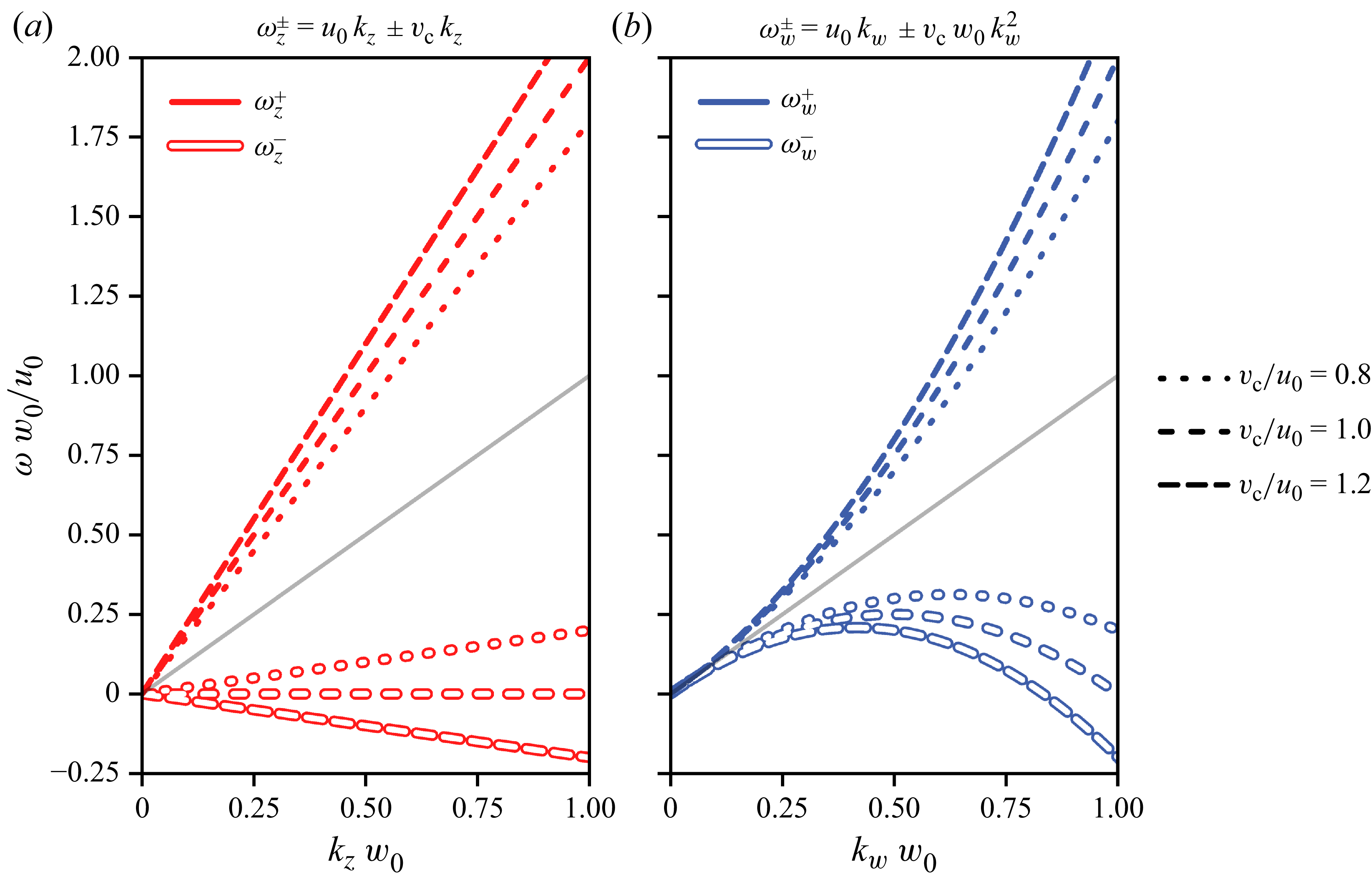
Each type of wave supports two modes, corresponding to the dispersion relations

(2.5a) \begin{align} \omega _{z}^{\pm } &= (u_0 \pm {v_{{c}}}) k_z ,\\[-9pt] \nonumber \end{align}

(2.5b) \begin{align} \omega _{w}^{\pm } &= u_0 k_w \pm {v_{{c}}} w_0 {k_w}^2 , \\[9pt] \nonumber\end{align}

which are plotted on figure 2.

Figure 2.

Dispersion relations of transverse (a) and longitudinal waves (b), in the absence of damping. The axis is made dimensionless through appropriate scaling. The horizontal axes correspond to the dimensionless wavevector amplitude $k\, w_0$ , while vertical axes correspond to the dimensionless angular frequency $\omega \, w_0/u_0$ . The grey lines correspond to pure advection $\omega = k\, u_0$ .

The transverse waves propagate non-dispersively, while the dispersion relation of the longitudinal waves display a quadratic term. For both waves, two branches coexist: one fast branch for which the phase speed in the laboratory reference frame is faster than the flowing speed $u_0$ ; and one slow branch which displays phase speeds in the laboratory reference frame inferior to $u_0$ (and which can be negative). These branches correspond, respectively, to positive (for fast waves) or negative (for slow waves) phase speed in the reference frame advected with the flow speed $u_0$ .

3.1. A pattern-forming instability

Consider the rivulet at rest in the vertical base state. Let us now impose an additive forcing which is homogeneous in space and harmonic in time. If the forcing exceeds a certain threshold, which depends on its frequency, a pattern starts to appear.

The speakers are driven in an antisymmetric configuration, so when one pushes its diaphragm out, the other pulls it in. This creates a pressure difference between both sides of the rivulet, displacing the liquid in the transverse direction. The rivulet thus behaves as a membrane, separating the cell into two airtight compartments. Note that since the speakers are not of infinite size, the forcing is not perfectly homogeneous: it is maximal on the midline joining the two speakers and slowly decreases away from it. All the measurements presented here are made on a 10 cm zone around this midline, where we checked that the forcing inhomogeneities never exceed ${10}{\,\%}$ .

The forcing of the rivulet by the pressure difference between its two sides is represented mathematically by the rightmost term in (2.1). This forcing is additive, meaning it induces a linear response from the rivulet. Thus, since the forcing oscillates harmonically in time at angular frequency $\omega _0$ , the rivulet adopts a movement that is homogeneous in space, and harmonic in time at angular frequency $\omega _0$ . This linear response is always visible on the experimental signal. Below the instability threshold, it is the only measurable evolution of $z(x, t)$ , but even when the instability develops, this response can still be seen by looking at $\langle {z}\rangle _x(t)$ , the space-averaged value of $z$ (see figure 3 a).

Figure 3.

Spatiotemporal representation of the experimental position $z(x,t)$ of the rivulet as a function of time and space. Cell gap $b={(0.58 \pm 0.02)}\,\textrm {mm}$ , flow rate $Q={(25.6 \pm 0.9)}\,\textrm {mm}^{3}\,\textrm {s}^{- 1}$ , excitation frequency $\omega _0/(2\pi )={40}\,\textrm {Hz}$ . (b) Position $z$ of the rivulet (colour scale) as a function of time $t$ and position $x$ . Darker regions delimited by plain lines correspond to the parts where the rivulet is the heaviest, while lighter regions delimited by dashed lines correspond to parts where the rivulet is the thinnest (see figure 4). (c) Time-averaged position (over 60 ms) of the rivulet as a function of space. Labelled ticks are spaced by $\lambda =2\pi /k = {6.74}\,\textrm {mm}$ . (a) Spaced-averaged position (over 17 mm) of the rivulet as a function of time. Labelled ticks are spaced by $2\pi /\omega _0 = {25.0}\,\textrm {ms}$ .

Above the instability threshold, the rivulet adopts a pattern composed of both transverse and longitudinal perturbations. As can be seen on figure 3(c), in addition to the time-dependent response to forcing the rivulet exhibits space-dependent transverse oscillations. The spatiotemporal transverse signal $z(x,t)$ is a combination of these two contributions. The rivulet also shows longitudinal oscillations, which as can be seen on figure 4 are a function of $x - v_w t$ , where $v_w = \omega _w^+ / k_w = u_0 + {v_{{c}}} w_0 k_w$ is the phase speed of longitudinal waves predicted by the dispersion relation (2.5b ). The observation of this pattern poses several questions, which motivate the present study. Let us highlight here some surprising key features of the experimental pattern we report, that will be explained theoretically in the following. The first and most obvious feature of the pattern is that, as can be seen for example on figure 3, both $z$ and $w$ share the same spatial periodicity. While this indicates that the two waves are probably coupled, the nature of such a coupling is not clear a priori. Second, the phase between the transverse and longitudinal patterns is deterministic (figure 3 b), which calls for an explanation. Third, the saturation amplitude of the patterns in $z$ and $w$ is unexplained, as is the ratio between these different perturbation – rephrased: Why are the transverse variations of greater amplitude than the longitudinal changes?

Figure 4.

Spatiotemporal representation of the experimental width $w(x,t)$ of the rivulet as a function of time and space. Cell gap $b={(0.58 \pm 0.02)}\,\textrm {mm}$ , flow rate $Q={(25.6 \pm 0.9)}\,\textrm {mm}^{3}\,\textrm {s}^{- 1}$ , excitation frequency $\omega _0/(2\pi )={40}\,\textrm {Hz}$ . (a) Width $w$ of the rivulet (colour scale) as a function of time $t$ and position $x$ . (b) Width of the rivulet interpolated along the plain black line represented on (a). The plain and dashed lines correspond to the width delimiting the darker and lighter regions on figure 3, respectively. The abscissa corresponds to a counter-advected position $x - v_w t$ , with $v_w={0}\,\textrm {mm}\,\textrm {s}^{- 1}$ the phase speed of longitudinal waves. Labelled ticks are spaced by $\sqrt {\lambda ^2 + (v_w T_0)^2}$ .

3.2. Mathematical formulation

In order to understand the instability and the pattern it generates, we write a nonlinear development of equations of (2.1) and (2.2), following a multiple scale approach (Nayfeh Reference Nayfeh2008; Bongarzone et al. Reference Bongarzone, Viola, Camarri and Gallaire2022). We will be using a slow time scale ${{ \tilde T }} = t /{{\epsilon }}^2$ , with ${{\epsilon }} \ll 1$ the small parameter introduced in the previous section. We also consider the case of weak forcing, that is to say we take the pressure difference imposed by the speakers $\varPi (t)$ to be of order ${{\epsilon }}^2$ .

At order ${\epsilon }$ , the equations read

(3.1a) \begin{align} {{\mathcal{L}_z}} z_1 &= 0 , \\[-9pt] \nonumber \end{align}

(3.1b) \begin{align} {{\mathcal{L}_w}} w_1 & = 0, \\[9pt] \nonumber \end{align}

i.e. at leading order $z(x,t) = {{\epsilon }} {{ \tilde Z }} e^{i(\omega _z t - k_z x)} + {\text{c.c.}}$ and $w(x,t) = {{\epsilon }} {{ \tilde W }} e^{i(\omega _w t - k_w x)} + {\text{c.c.}}$ , where $\text{c.c.}$ stands for complex conjugate, with $(\omega _z, k_z)$ satisfying the transverse waves dispersion relation (2.5a ) and $(\omega _w, k_w)$ satisfying the longitudinal waves dispersion relation (2.5b ).

At second order in ${\epsilon }$ , the equations read

(3.2a) \begin{align} w_0 {{\mathcal{L}_z}} z_2 & = {{\mathcal{N}_{z}}} (z_1, w_1, u_1) + \varPi (t), \\[-9pt] \nonumber \end{align}

(3.2b) \begin{align} {{\mathcal{L}_w}} w_2 & ={{\mathcal{N}_{w}}} (z_1, w_1, u_1), \\[9pt] \nonumber\end{align}

where ${{\mathcal{N}_{z}}} (z_1, w_1, u_1)$ and ${{\mathcal{N}_{w}}} (z_1, w_1, u_1)$ are quadratic nonlinear functions, the expression of which is given in Appendix A.2; and $\varPi (t) = \tilde {\varPi } e^{i\omega _0 t} + {\text{c.c.}}$ is the externally imposed pressure oscillation, homogeneous in space and harmonic in time, of amplitude $\tilde {\varPi }$ . The nonlinear terms ${{\mathcal{N}_{z}}} (z_1, w_1, u_1)$ and ${{\mathcal{N}_{w}}} (z_1, w_1, u_1)$ contain no contributions able to resonate with $z_1$ and $w_1$ . This can be seen by looking directly at the expressions or by considering symmetry arguments. Equation (3.2) thus reduce to

(3.3a) \begin{align} -w_0 {\omega _0}^2 z_2 &= \tilde {\varPi } e^{i\omega _0 t} + {\text{c.c.}}, \\[-9pt] \nonumber \end{align}

(3.3b) \begin{align} w_2 &= 0, \\[9pt] \nonumber\end{align}

the forcing only adds an additive contribution to the transverse pattern,

(3.4) \begin{align} z(x,t) = {{\epsilon }} {{ \tilde Z }} e^{i(\omega _z t - k_z x)} + {{\epsilon }}^2 {{ \tilde F }} e^{ i(\omega _0 t - 0x)}+ {\text{c.c.}} \,\, \text{and}\,\,\, w(x,t) = {{\epsilon }} {{ \tilde W }} e^{i(\omega _w t - k_w x)} + {\text{c.c.}} \end{align}

The term proportional to ${{\epsilon }}^2 {{ \tilde F }}$ on the expression of $z(x,t)$ corresponds to the linear response to the forcing. The expression of the operator ${\mathcal{L}_z}$ allows us to write an explicit expression for ${ \tilde F }$ , defined as ${{ \tilde F }} := - \tilde {\varPi } / (w_0\,{\omega _0}^2)$ .

At third order in ${\epsilon }$ , elimination of the resonant terms leads to the following amplitude equations:

(3.5a) \begin{align} 2\partial _{{ \tilde T }} {{ \tilde Z }} =& -\mu \left ( 1 + \varepsilon _z \frac {{\mu _{{cl}}}}{w_0 \mu } (1 + \varepsilon _z )\right ) {{ \tilde Z }} - i \varepsilon _z \frac {{\omega _0}^2}{w_0 u_0 k_w} {{ {{{ \tilde F }}}^* }} {{ \tilde W }} \nonumber \\ & + 7 i {k}^3 u_0 |{ \tilde Z }|^2 {{ \tilde Z }} + i {k}^3 u_0 \left (- \varepsilon _z \frac 54 + \frac {4 \varepsilon _w}{kw_0}\right ) |{ \tilde W }|^2 {{ \tilde Z }} , \\[-9pt] \nonumber\end{align}

(3.5b) \begin{align} 2\partial _{{ \tilde T }} {{ \tilde W }} =& - \mu {{ \tilde W }} - i \varepsilon _w k_w \omega _0 \left ( \frac {{\omega _0}}{k_w {v_{{c}}}} -\varepsilon _w w_0 k_z \right ) {{ \tilde F }} {{ \tilde Z }} \nonumber \\ & -2 i \varepsilon _w w_0 {k_w}^2 {v_{{c}}} |{k_z{{ \tilde Z }}}|^2 {{ \tilde W }} + i \left ( k_w\frac {u_0}{{w_0}^2} -\varepsilon _w \frac 32 w_0 {v_{{c}}} {k_w}^4 \right ) {|{{ \tilde W }}|}^2 {{ \tilde W }}, \\[12pt] \nonumber \end{align}

where ${ {A}^* }$ denotes the complex conjugates of $A$ and $\varepsilon _{z,w}$ are each to be replaced by $+1$ or $-1$ , depending on the chosen propagation dispersion ( $\varepsilon _w = \pm 1$ for $\omega _w^\pm$ , and similarly for $\varepsilon _z$ ). The main steps allowing the derivation of (3.5) are shown in Appendix A.3. For the equations presented in the made text we made the simplifying assumption ${v_{{c}}} \approx u_0$ , the full expression of $\partial _{{ \tilde T }} {{ \tilde Z }}$ and $\partial _{{ \tilde T }} {{ \tilde W }}$ in the general case is presented in Appendix A.3. Let us now try to get a physical understanding of these equations. The right-hand side comprises three kinds of terms: dissipative linear damping, nonlinear cross-coupling and third-order nonlinearities, in this order.

For longitudinal waves the linear damping is always the same, while for transverse waves the damping depends on the branch considered. When $\varepsilon _z = -1$ ( $\omega _z^-$ branch) the multiplicative coefficient for the linear term is $-\mu$ , but the $\varepsilon = +1$ ( $\omega _z^+$ branch) is subject to a much more important attenuation, with a coefficient $-\mu (1 + 2{\mu _{{cl}}}/(w_0\,\mu ))$ . Indeed, since the rivulet is thin, the dissipation due to transverse menisci displacement dominates the bulk dissipation: ${\mu _{{cl}}} \gg w_0 \mu$ , meaning that the $\omega _z^+$ branch is strongly damped. Let us physically explain this dependence of dissipation with the phase velocity.

In general, since the rivulet is thin, the dissipation due to the displacement of the transverse menisci dominates the dissipation in the volume: ${\mu _{{cl}}} \gg w_0 \mu$ , the main part of the energy loss comes from the ‘friction’ of the menisci on the glass plates that delimit the cell. A wave on the $\omega _z^-$ branch moves at the velocity $u_0 - {v_{{c}}}$ in the laboratory frame, thus with respect to the plates. This velocity is very small (compared with $u_0$ or $v_{{c}}$ , which are of the same order of magnitude), so the menisci are almost motionless with respect to the plates and therefore generate very little friction. On the contrary, if we consider a wave on the $\omega _z^+$ branch, the rivulet slides on the plates at the velocity $u_0+{v_{{c}}}$ in the laboratory frame, and the menisci are displaced rapidly with respect to the plates, which is energetically costly. The $\omega _z^+$ branch is therefore strongly damped: this is consistent with the fact that transverse waves $\omega _z^+$ are never observed experimentally. For the following we will thus only consider the case $\varepsilon _z = -1$ . The fact that the damping then becomes exactly the same for transverse and longitudinal waves is a consequence of the simplifying ${v_{{c}}} \approx u_0$ assumption.

The most interesting parts of (3.5) are undoubtedly the cross-coupling terms, which imply an interaction between transverse and longitudinal waves. The sign of each nonlinear coupling term is critical for the amplification mechanism, and it can only be obtained through a careful derivation of the third-order equations. As we will show rigorously in § 4.2, the interaction of transverse and longitudinal waves is only constructive if the product of both coupling terms is of positive sign, in the opposite case the interaction only leads to increased damping for both waves. In order to observe an instability, we must thus have $(-i \varepsilon _z)(- i \varepsilon _w) = +1$ (assuming $\omega _0 \gg {v_{{c}}} w_0 k^2$ , which is always verified in the accessible experimental range). Since $\varepsilon _z = -1$ , this forces $\varepsilon _w = +1$ to be the branch amplified by the instability.

Looking at figure 3, one can confirm that the prediction $(\varepsilon _z, \varepsilon _w) = (-1, +1)$ is well verified experimentally: we can see that $\omega _w \gt \omega _z$ , with $v_z = \omega _z/k_z \approx 0$ .

Note that the form of the coupling term is a signature that the instability is indeed parametric, as the forcing response ${ \tilde F }$ acts as a multiplicative parameter coupling the two waves together. The fact that the linear response to an additive forcing intervenes multiplicatively in the amplitude equations participates in the instability originality. This coupling between two waves mediated by a forcing is analogous to the cross-coupling between progressive and regressive waves in the Faraday instability in an annulus (Douady et al. Reference Douady, Fauve and Thual1989).

The rightmost terms of the (3.5) are nonlinear detuning terms. Indeed in the absence of nonlinear damping, these terms are associated with a purely imaginary prefactor, translating the fact that as the amplitudes of the waves grow, their frequencies shift accordingly. These detuning terms are often responsible for the nonlinear saturation of parametric instabilities, because they shift the oscillation frequency away from resonance.

To conclude this section, note that the general form of (3.5) could have been guessed by using only symmetry arguments. If one assumes that the evolution equations for ${ \tilde Z }$ and ${ \tilde W }$ contain only third-order terms proportional to ${ \tilde Z }$ , ${ \tilde W }$ , ${ \tilde F }$ and their complex conjugates, then necessarily such terms must be compatible with the invariances and symmetries of the problem.

Let us consider the time translation invariance of the problem, i.e. the fact that the equations should not change when the transformation $t\rightarrow t + t_0$ is applied. This transformation corresponds, in terms of our variables, to the phase shift ${{ \tilde Z }}, {{ \tilde W }}, {{ \tilde F }} \rightarrow {{ \tilde Z }} e^{i\phi }, {{ \tilde W }} e^{i\phi + i\psi }, {{ \tilde F }} e^{i\psi }$ with $\phi = \omega _z t_0$ and $\psi = \omega _0 t_0$ . The third-order evolution equations, in order to be invariant under this transformation, must then have the following form:

(3.6a) \begin{align} \partial _{{{ \tilde T }}}{{ \tilde Z }} = a \mu {{ \tilde Z }} + b {{ {{{ \tilde F }}}^* }} {{ \tilde W }} + c {{ \tilde Z }}^2 {{ {{{ \tilde Z }}}^* }} + d {{ \tilde W }} {{ {{{ \tilde W }}}^* }}{{ \tilde Z }}, \\[-9pt] \nonumber \end{align}

(3.6b) \begin{align} \partial _{{{ \tilde T }}}{{ \tilde W }} = a' \mu {{ \tilde W }} + b' {{ \tilde F }} {{ \tilde Z }} + c' {{ \tilde Z }}{{ {{{ \tilde Z }}}^* }}{{ \tilde W }} + d' {{ \tilde W }}^2 {{ {{{ \tilde W }}}^* }}, \\[9pt] \nonumber \end{align}

which is indeed the same form as (3.5).

Finally, the space–time reversal symmetry $x, t\rightarrow -x, -t$ , imposes the phase (the real or imaginary character) of the prefactors $a,b, c, d, a', b', c'$ and $d'$ , since it corresponds to the transformation ${{ \tilde Z }}, {{ \tilde W }}, {{ \tilde F }} \rightarrow {{ {{{ \tilde Z }}}^* }}, {{ {{{ \tilde W }}}^* }}, {{ {{{ \tilde F }}}^* }}$ and $\mu \rightarrow -\mu$ .

3.3. Resonance condition

Since (3.5) result from the elimination of secular terms, one can see that the cross-coupling terms can only be taken into account if a certain resonance condition is met. Indeed, for the coupling term ${{ \tilde F }} e^{ i(\omega _0 t - 0x)} {{ \tilde Z }} e^{i(\omega _z t - k_z x)} = {{ \tilde F }} {{ \tilde Z }} e^{i((\omega _z + \omega _0)) t - (k_z+0) x)}$ to interact with the longitudinal wave ${{ \tilde W }} e^{i(\omega _w t - k_w x)}$ , both terms must oscillate at the same (spatial and temporal) frequency. The resonance, or frequency-matching condition, translates to the fact that the interaction between the waves have to be resonant for them to exchange energy and potentially amplify one another.

This behaviour is analogous to a three-wave resonant interaction, where an algebraic relationship must be satisfied between the waves for the triadic interaction to take place (Simmons Reference Simmons1969; Martin, Simmons & Wunsch Reference Martin, Simmons and Wunsch1972; Phillips Reference Phillips1981; Hammack & Henderson Reference Hammack and Henderson1993). It is this mechanism which is responsible, for example, for pattern generation due to nonlinear interaction between gravitocapillary surface waves (Mcgoldrick Reference Mcgoldrick1965; Moisy et al. Reference Moisy, Michon, Rabaud and Sultan2012; Haudin et al. Reference Haudin, Cazaubiel, Deike, Jamin, Falcon and Berhanu2016). Here the waves are a transverse wave, a longitudinal wave and the ${{ \tilde F }} e^{i\omega _0 t} + {\text{c.c.}}$ contribution to $z(x,t)$ (linear response to forcing), which can be thought of as a zero-wavenumber transverse wave.

The resonance condition thus mathematically reads

(3.7a) \begin{align} \omega _w&-\omega _z = \pm \omega _0, \\[-9pt] \nonumber\end{align}

(3.7b) \begin{align} k_w&-k_z=\pm 0, \\[9pt] \nonumber\end{align}

since both temporal and spatial frequencies must match for resonance to take place. Equation (3.7a , b ) impose a necessary condition to the existence of the cross-coupling term, and thus of the instability. They have straightforward implications for the pattern features. Equation (3.7b ) provides a theoretical explanation for the fact that both transverse and longitudinal waves share the same wavenumber, and thus the same spatial wavelength. Equation (3.7a ) predicts a deterministic relation between the different frequencies. The quantity $\omega _w - \omega _z$ can take two values, depending on the value of the product $\varepsilon _-\varepsilon _+$ . The result is plotted on figure 5. They show an excellent agreement with our prediction, that the excited modes are the $\omega _w^+, \omega _z^-$ modes.

Figure 5.

Relationship between $k$ and $\omega _0$ . Symbols correspond to experimental measurements of the wavenumber $k$ (which is the same for transverse and longitudinal waves). Experiments done with cell gap $b={0.6}\,\textrm {mm}$ and flow rate $Q={(26 \pm 1)}\,\textrm {mm}^{3}\,\textrm {s}^{- 1}$ . Lines correspond to $|{\omega _w^+ - \omega _z^-}| = k{v_{{c}}} (1 + k w_0)$ , i.e. $\varepsilon _z\varepsilon _w = -1$ (purple) and $|{\omega _w^- - \omega _z^-}| = k{v_{{c}}} |{1 - k w_0}|$ , i.e. $\varepsilon _z\varepsilon _w = +1$ (ochre). The line curves are computed without fitting, using the experimental values of the parameters. The theoretical prediction corresponds to the modes $\omega _w^+, \omega _z^-$ being unstable (purple curve). Note that the experimental points often fall slightly to the right of the curve, i.e. the wavevectors $k$ are larger than expected: this is because the points were recorded at a finite amplitude for which nonlinear detuning is measurable (see § 4.4).

Note that the structure of these equations explain simply why it is possible to observe the instability in a very wide range of excitation frequency. Indeed, the curve $\omega _0 = \omega _w^+ - \omega _z^-$ as a function of $k$ maps $\mathbb{R}$ to itself: for every excitation frequency $\omega _0$ , there exists a wavenumber $k$ for which the resonance condition can be fulfilled. Experimentally, we could not observe the instability using frequencies below 10 Hz, for in such condition the wavelength becomes comparable to the size over which the forcing is homogeneous.

3.4. Physical interpretation of the instability mechanism

Let us now try to convey a qualitative understanding of the physical effects represented by the nonlinear coupling terms of (3.5) responsible for the destabilization of the straight rivulet.

One interesting feature of the present instability is that neither of the two types of waves in the final pattern is unstable on its own in the absence of forcing, nor does the forcing directly amplify any of the perturbation. While sinuous and varicose instabilities are often present in fluid mechanics, for example when studying jets (Eggers & Villermaux Reference Eggers and Villermaux2008; Mikhaylov & Wu Reference Mikhaylov and Wu2020) or sheets (Villermaux & Clanet Reference Villermaux and Clanet2002), usually either one mode becomes unstable on its own, or two or more modes become unstable, compete for energy and the fastest growing mode wins. In the system we study here, the forcing only acts as a mere intermediary, as its only role is to couple together two different type of waves which would not interact in the absence of forcing. The two coupling terms in (3.5a ) and (3.5b ) are mathematical representations of the two ways that longitudinal and transverse waves can influence one another.

The ${{ {{{ \tilde F }}}^* }}{{ \tilde W }}$ term in (3.5a ) that governs the evolution of the path ${ \tilde Z }$ translates the fact that a rivulet with uneven width will see its path deformed when displaced transversally under the action of the forcing, as illustrated on figure 6(a). Indeed, if a rivulet presenting width modulations is moved transversally, then the thicker parts of the rivulet, having more inertia, will be less mobile than the thinner parts of the rivulets, which carry a lesser mass of liquid. Since different parts of the rivulet, having different mass, will displace transversally along different lengths, this will lead to a deformation of the path followed by the rivulet. Following this reasoning, it is straightforward that the spatial periodicity of the path deformation will be the same as the width modulation periodicity. This allows for a qualitative understanding of condition (3.7b ) (the two waves share the same wavelength).

Figure 6.

Schematic illustration of the crossed-amplification mechanism. The length of the arrows represents the intensity of the displacement locally imposed to the rivulet. (a) Deformation of the fluid path due to space-varying mass repartition on the rivulet. (b) Change in the width profile due to the rivulet path being non-straight. Note that as the forces are drawn, the sinuose and varicose deformation enhance each other. If the directions of the arrows are reversed but the sinuosity stays the same (corresponding to a change of sign in force while staying in the reference frame moving with the sinuosity, i.e. to transformation (3.8)), then the interaction only stays constructive if the width modulation is moved half a wavelength downwards, i.e. (3.9) must be verified. (See also Supplementary figure SF1.)

The ${{ \tilde F }}{{ \tilde Z }}$ term in (3.5b ) that governs the evolution of the width perturbation ${ \tilde W }$ represent the fact that a rivulet with a curved path will see its width profile evolve when displaced under the action of the forcing, as illustrated on figure 6(b). Let us considering a rivulet presenting a period curved path, being moved like a membrane under the action of differential pressure between both sides of the rivulet. At places where the curvature is of the same sign as the pressure displacement force, the fluid will accumulate, being drawn in from the sides, and the rivulet will get thicker. On the contrary, places where the curvature is of opposite sign as the pressure force will be depleted in fluid and will be getting thinner, for the same reason the membrane of an expanding rubber balloon thins. As before, following this reasoning we also understand that the spatial periodicity of the width modulation will reflect that of the path curvature, validating once more condition (3.7b ).

Finally, let us considers the same mechanisms that were just exposed in the two preceding paragraphs, but half a forcing period later, as is shown on the bottom part of Supplementary figure SF1. This corresponds to changing the sign of the pressure force/transverse displacement: formally, this is associated with the

(3.8) \begin{align} t\rightarrow t+ \pi /\omega _0 && \tilde {\varPi } \rightarrow -\tilde {\varPi } && {{ \tilde F }} \rightarrow -{{ \tilde F }} && {{ \tilde Z }}\rightarrow {{ \tilde Z }} e^{i\pi \omega _z/\omega _0} && {{ \tilde W }}\rightarrow {{ \tilde W }} e^{i\pi \omega _w/\omega _0} \end{align}

transformation. The varicose amplification mechanism will lead to a width modulation of opposite sign compared with the previous situation (since the pressure drop changed sign). In order for the total mechanism to work this must be on par with the action of the sinuosity amplification mechanism, which requires the width modulation pattern to be displaced by half a wavelength compared with the sinuous pattern (see Supplementary figure SF1 for an illustration): formally, this corresponds to the

(3.9) \begin{align} {{ \tilde W }}\rightarrow -{{ \tilde W }} e^{i\pi \omega _z/\omega _0} = {{ \tilde W }} e^{i\pi (\omega _z \pm \omega _0)/\omega _0} \end{align}

transformation. Hence, for the mechanism to work at all times, the system must verify $\omega _w = \omega _z \pm \omega _0$ : this is precisely the resonance condition (3.7a ). Both resonance conditions can thus be understood qualitatively by looking at the physical interpretation of the amplification mechanism: two different effects combine to form the complete amplification cycle.

One obvious follow-up question following this demonstration would be: What is the relative importance of these two effects? This question, and others, finds its answer in the next section.

4.1. Dimensionless formulation

In order to make the mathematical computations more concise, we use changes of variables to make the system of equations dimensionless. The time scale choice is straightforward and corresponds to $2/\mu$ , the typical wave damping time in the absence of forcing. As length scale we choose the quantity ${{ \ell }} := \mu \sqrt {w_0 {v_{{c}}} / {\omega _0}^3}$ , the interpretation of which will become clear in the next subsection. Thus, we define

(4.1) \begin{align} T := \mu {{ \tilde T }}/2 && {{ F }} := {{ \tilde F }}/{{ \ell }} && {{ Z }} := {{ \tilde Z }}/{{ \ell }} && {{ W }} := {{ \tilde W }}/{{ \ell }} \end{align}

which allows us to write (3.5) in a compact dimensionless form

(4.2a) \begin{align} \partial _T Z &= - Z + i \phi {{ {F}^* }} W + i \big (\alpha _{ZZ} {|Z|}^2+ \alpha _{ZW} {|W|}^2 \big )Z , \\[-9pt] \nonumber\end{align}

(4.2b) \begin{align} \partial _T W &= - W - i\frac {1}{\phi } F Z + i \big (\alpha _{WZ} {|Z|}^2+ \alpha _{WW} {|W|}^2 \big )W, \\[9pt] \nonumber \end{align}

where $\phi := ({1}/{u_0 k})(\sqrt { {\omega _0{v_{{c}}}}/{w_0}})$ ; and the detuning prefactors $\alpha _{XX}$ are defined as follows:

(4.3) \begin{align} \alpha _{ZZ} &:= 7\,\varXi \,(k w_0)^3, & \alpha _{ZW} &:= 4 \varXi \,(k w_0)^2 \left (1 + \frac {5}{16} (k w_0)\right )\!, \nonumber \\ \alpha _{WZ} &:= 2\,\varXi \,\frac {{v_{{c}}}}{u_0} (k w_0)^4, & \alpha _{WW} &:= \varXi \,k w_0,\end{align}

where $\varXi := {\mu u_0{v_{{c}}}}/{{\omega _0}^3{w_0}^2} = {u_0 {{ \ell }}^2}/{\mu {w_0}^3}$ characterizes the detuning strength. The dimensionless coefficient $\phi$ translates the relative efficacy of the two effects that participate in the coamplification: amplification of sinuosity due to uneven mass repartition, and amplification of varicosity due to path curvature (see § 3.4 for further details on the physical interpretation of these terms). It thus quantifies the asymmetry of the instability mechanism: thick rivulets moved at low frequency have $\phi \gg 1$ and are unstable because of the path deformation due to width heterogeneity, while thin rivulets moved at high frequency have $\phi \ll 1$ and are mostly unstable because of curvature induced fluid concentration along the rivulet. All the experiments presented in this study display $\phi \gt 1$ , meaning that the main amplification stage in the mechanism is the differential movement of the path due to the spatially inhomogeneous inertia of the rivulet.

4.2. Instability threshold

We will now turn to the study of the pattern near the instability threshold: in all the following, we will assume ${|Z|} \sim {{\epsilon '}}$ and ${|W|} \sim {{\epsilon '}}$ , with ${{\epsilon '}}\ll 1$ . We define the vector $| {U}\rangle := \begin{pmatrix} Z \\ W\end{pmatrix} $ which condenses all the information about the state our system is in, using a concise notation. We borrow the bra–ket notation to our quantum mechanics colleagues as it is particularly useful when dealing with linear algebra problems. Since $\|{U}\| \ll 1$ , (4.2a ) and (4.2b ) can be simplified to

(4.4) \begin{align} \partial _T| {U}\rangle &= {{\mathbf{L}}}| {U}\rangle, \quad \text{with}\quad {{\mathbf{L}}}=\left (\begin{matrix}-1 & i\phi {{ {F}^* }}\\-i \frac 1\phi F & -1\end{matrix}\right ) \end{align}

being a linear evolution operator.

The trace of the matrix ${\boldsymbol{L}}$ is $\textrm {tr} ({{\boldsymbol{L}}}) = -2 \lt 0$ . Since it is the sum of the eigenvalues ${\boldsymbol{L}}$ , we can conclude that there always exists at least one mode that is linearly damped. The determinant reads $\Delta ({{\boldsymbol{L}}}) = 1 - {|F|}^2$ , it is the product of the eigenvalues of ${\boldsymbol{L}}$ . The instability develops if and only if one mode is linearly amplified, i.e. if one of the eigenvalues of ${\boldsymbol{L}}$ has a positive real part. This is only the case if $\Delta ({{\boldsymbol{L}}})$ is negative, which happens when the forcing exceeds a critical threshold equal to one in dimensionless units. The instability thus develops if and only if the condition

(4.5) \begin{align} {|F|}^2 \gt {|{ F _c}|}^2 := 1 \quad \Leftrightarrow \quad {|{\tilde F}|} \gt {{|{\tilde F}|}_c} := \mu \sqrt {\frac {w_0 {v_{{c}}} }{ {\omega _0}^3}} = {{ \ell }} \end{align}

is fulfilled. The interpretation of ${ \ell }$ is now clear: it corresponds to the minimum transverse displacement needed to develop the instability. This provides us with a scaling law for the threshold forcing amplitude: ${|{\tilde F_c}|} \propto (\omega _0)^{-3/2}$ . This scaling law is shown on figure 7 to be verified by experimentally. Interestingly, the prefactor value obtained by computing the best fit (33.7 $\textrm {mm}\times \textrm {Hz}^{-3/2}$ ) is the same order of magnitude but does not correspond exactly to the theoretical prefactor computed using the analytical formula (4.5) ( ${(16.4 \pm 3,3)}{\,\textrm {mm}\times \textrm {Hz}^{-3/2}}$ ). Several factors may explain this discrepancy. On the experimental side, the precise measurement of ${|{\tilde F_c}|}$ itself is difficult, especially at high frequencies. On the theoretical side, this difference may be explained, partially or totally, by several factors: the ${{\epsilon }} \ll 1$ approximation, which is not strictly respected in the developed pattern, the weakly nonlinear method we use, if the nonlinearity is more important than anticipated or the $u_0\approx {v_{{c}}}$ approximation, which is not exact. The fact that the best fit value is almost exactly a factor two off the theoretical result could also indicate an algebraic error in our computations, even though we could not catch it after rederiving our results several times.

Figure 7.

Threshold transverse displacement as a function of excitation frequency. Experiments done with cell gap $b={0.6}\,\textrm {mm}$ and flow rate $Q={(26 \pm 1)}\,\textrm {mm}^{3}\,\textrm {s}^{- 1}$ . The black dots correspond to experimental measurements. The dashed grey line represents the resolution limit of our measurement method; it corresponds to one fifth of the pixel spacing. The full green line is a one-parameter fit corresponding to a power law of exponent $-3/2$ , the multiplicative factor being free. Inset: same data on a log–log scale.

4.3. Pattern structure

After identifying the forcing threshold over which the instability develops, we now turn to the study of the pattern itself. We ought to understand the structure of the most unstable mode that grows, and compare it with the pattern observed in the experiments.

To do so, we place ourselves in the vicinity of the instability threshold, assuming $F = F_c + {{\epsilon '}}^2\delta F$ with ${|{F_c}|} = 1$ and ${\epsilon '}$ the small parameter introduced in the previous subsection. This allows us to decompose the evolution matrix into

(4.6) \begin{align} {{\boldsymbol{L}}} = {{{{\boldsymbol{L}}}_0}} + {{\epsilon '}}^2 {{ \delta {{\boldsymbol{L}}} }} = \left (\begin{matrix}-1 & i\phi {{ {F_c}^* }} \\-i \frac 1\phi F_c & -1\end{matrix}\right ) + {{\epsilon '}}^2 i \left (\begin{matrix}0 & \phi {{ {\delta F}^* }} \\- \frac 1\phi \delta F & 0\end{matrix}\right )\!. \end{align}

The matrix ${{{\boldsymbol{L}}}_0}$ is diagonalizable and has two eigenvalues, $\lambda _0 = 0$ and $\lambda _- = -2$ , associated with the two eigenvectors

(4.7) \begin{align} |{V_0}\rangle = \frac {1}{\sqrt {1 + {|{F_c}|}^2/\phi ^2}}\left (\begin{matrix}1 \\-i F_c/\phi \end{matrix}\right ) && \,\,\,\text{and}\,\,\, && | {V_-}\rangle = \frac {1}{\sqrt {1 + \phi ^2{|{F_c}|}^2}}\left (\begin{matrix}-i \phi {{ {F_c}^* }} \\1\end{matrix}\right ) \end{align}

which are of norm 1, using the standard product $\langle{P}|{Q}\rangle = P^\dagger \, Q$ where $P^\dagger$ represents the adjoint, or transconjugate, of $P$ .

The eigenvector $| {V_0}\rangle$ corresponds to a neutral mode of the operator ${{{\boldsymbol{L}}}_0}$ . It is the mode that will be amplified and that saturates when nearby the threshold instability. Thus, we can write, at first order in ${\epsilon '}$ , $| {U}\rangle = {{\epsilon '}} A | {V_0}\rangle$ with $A$ being the dimensionless amplitude of the pattern.

Looking at $| {V_0}\rangle$ , it is thus possible to obtain information about the structure of this neutral mode. In particular, if the pattern is given by $| {V_0}\rangle$ , then we can write the following relationship between $Z$ and $W$ :

(4.8) \begin{align} W = -i \frac {F_c}{\phi }Z \end{align}

where here the $\phi$ factor translates the fact that since one mechanism is more efficient than the other, then one of the waves will have greater amplitude. Indeed, in the experimental pattern (figures 3 and 4) we observe that the transverse waves have a greater amplitude than the longitudinal waves, which is coherent with the fact that the $\phi$ factor is always greater than one in the experiments we show in this article. Equation (4.8) contains all the information about the structure of the instability pattern. Taking the argument and the norm, we can write

(4.9a) \begin{align} \arg W &= \arg {Z} + \arg {F} - \frac {\pi }{2}, \end{align}

(4.9b) \begin{align} {|W|} &= {|Z|}/\phi = k {|Z|}\ u_0\sqrt {w_0 / (\omega _0\,{v_{{c}}})} .\end{align}

Equation (4.9a ) predicts the relative phase between the longitudinal wave, the transverse wave and the response to forcing. The arguments of $Z$ , $F$ and $W$ correspond to three degrees of freedom of the system. Since any pair of these can be arbitrarily changed by redefining the origins of space (by the transformation $x \rightarrow x+ x_0$ ) and time (by the transformation $t \rightarrow t+ t_0$ ), this relation completely constrains the system. As can be seen on figure 8(a), the relation (4.9a ) is verified experimentally with excellent precision. Note that signature of this phase relation can be seen when observing directly the pattern. For example, on figure 3, extrema of $w$ (centre of dark or light shaded zones in the central plot, corresponding to $\arg (W) \equiv 0 [\pi ]$ ) are never found in places where $z$ is extremal (i.e. where $\arg (Z) + \arg (F) \equiv 0 [\pi ]$ ). On the same figure, by looking carefully at the intersections between extrema of $w$ , extrema and zeros of $Z$ (figure 3 a), and extrema and zeros of $F$ (figure 3 c), one can recover (4.9a ).

Figure 8.

Structure of the combined mode. The dots always correspond to experimental measurement. Cell gap $b={(0.58 \pm 0.02)}\,\textrm {mm}$ , flow rate $Q={(25.6 \pm 0.9)}\,\textrm {mm}^{3}\,\textrm {s}^{- 1}$ , excitation frequency $\omega _0/(2\pi )={40}\,\textrm {Hz}$ . (a) Relative phase of the waves as a function of the transverse movement amplitude. There are measurement points below the threshold where we can still observe a weak pattern (see discussion on § 4.4). (b) Link between the relative amplitude of transverse and longitudinal waves as a function of the transverse movement amplitude. The points below the threshold are associated with high experimental uncertainty, since the associated amplitudes are very small (see figure 9).

Complementary to (4.9a ), relationship (4.9b ) predicts the relative amplitude between the two waves forming the pattern. The norms of $Z$ , $F$ and $W$ correspond to three degrees of freedom of the system. The amplitude of $F$ is directly imposed by the forcing, and the pattern amplitude $|A|$ depends on nonlinear saturation effects, hence (4.9b ) closes the system and determines completely the pattern. As one can see on figure 8(b), this relationship is very well recovered by the experiments.

In order to completely characterize the instability, we still need to understand the saturation of the pattern amplitude $A$ , which is the object of the next subsection.

4.4. Nonlinear detuning and saturation

We now turn to finer effects due to nonlinear terms: frequency detuning and amplitude saturation. To do so, we allow the amplitude $A$ to vary with a slow dimensionless time scale $\tau = T / {{\epsilon '}}^2$ , so that (4.2a ) and (4.2b ) can be written, up to third order in ${\epsilon '}$ , in the form

(4.10) \begin{align}\partial _{\tau }| {U}\rangle = ({{{{\boldsymbol{L}}}_0}} + {{\epsilon '}}^2 {{ \delta {{\boldsymbol{L}}} }})| {U}\rangle+ i \left (\begin{matrix}\alpha _Z & 0 \\ 0 & \alpha _W\end{matrix}\right ) {{\epsilon '}}^2{|A|}^{2} | {U}\rangle\end{align}

where we defined $\alpha _z$ so that

(4.11) \begin{align} {{\epsilon '}}^2{|A|}^2 \alpha _Z = \alpha _{ZZ}{|Z|}^2 + \alpha _{ZW}{|W|}^2 = {{{\epsilon '}}^2 {|A|}^2} \frac {\alpha _{ZZ} + \alpha _{ZW} {|{F_c}|}^2 /\phi ^2}{1 + {|{F_c}|}^2 /\phi ^2} \end{align}

and similarly so for $\alpha _W$ . We also have to expand $| {U}\rangle$ in powers of ${\epsilon '}$ : $| {U}\rangle = {{\epsilon '}} | {U_1}\rangle + {{\epsilon '}}^2| {U_2}\rangle + {{\epsilon '}}^3| {U_3}\rangle+ \ldots$ (4.10) at order one which yields the familiar result $| {U_1}\rangle = A(\tau )| {V_0}\rangle$ . By going to higher order, we are now searching to characterize the evolution of $A$ with $\tau$ . At order two the equation leads to $| {U_2}\rangle = | {0}\rangle$ , while the third-order development yields

(4.12) \begin{align} \partial _{\tau }A | {V_0}\rangle = {{{{\boldsymbol{L}}}_0}}| {U_3}\rangle + A {{ \delta {{\boldsymbol{L}}} }}| {V_0}\rangle+ i {|A|}^{2}A\left (\begin{matrix}\alpha _Z & 0 \\ 0 & \alpha _W\end{matrix}\right ) | {V_0}\rangle , \end{align}

which can be rewritten in the form

(4.13) \begin{align} | {N}\rangle := {{{{\boldsymbol{L}}}_0}}| {U_3}\rangle = \partial _{\tau }A | {V_0}\rangle - iA \left (\begin{matrix}0 & \phi {{ {\delta F}^* }}\\ -\frac 1\phi \delta F & 0\end{matrix}\right ) | {V_0}\rangle - i {|A|}^{2}A\left (\begin{matrix}\alpha _Z & 0 \\0 & \alpha _W\end{matrix}\right ) | {V_0}\rangle\ . \end{align}

Using the Fredholm alternative, we find that $| {N}\rangle$ must be orthogonal to the kernel of ${{{{\boldsymbol{L}}}_0}}^\dagger$ . This can be justified using the simple following reasoning: a weak writing of the equality ${{{{\boldsymbol{L}}}_0}}| {U_3}\rangle = | {N}\rangle$ is that any vector $| {P}\rangle$ must verify $\langle{P}|{N}\rangle = \langle{P}| {{{{\boldsymbol{L}}}_0}}| {U_3}\rangle = \langle{U_3}|{{{{{\boldsymbol{L}}}_0}}}^\dagger | {P}\rangle$ . In particular, if $| {P}\rangle \in \ker ({{{{{\boldsymbol{L}}}_0}}}^\dagger )$ , that is to say if ${{{{{\boldsymbol{L}}}_0}}}^\dagger | {P}\rangle = 0$ , then $\langle{P}|{N}\rangle = 0$ , recovering that $| {P}\rangle$ is orthogonal to $| {N}\rangle$ .

The kernel of ${{{{{\boldsymbol{L}}}_0}}}^\dagger$ is the span of the vector $| {W_0}\rangle$ , the eigenvector of ${{{{{\boldsymbol{L}}}_0}}}^\dagger$ of norm unity associated with the zero-eigenvalue

(4.14) \begin{align} | {W_0}\rangle := \frac {1}{\sqrt {1 + \phi ^2{F_c}^2}}\left (\begin{matrix}1 \\ -i \phi F_c\end{matrix}\right ) \end{align}

which resembles closely $| {V_0}\rangle$ since ${\boldsymbol{L}}$ is close to a Hermitian. The condition $\langle{W_0}|{N}\rangle = 0$ yields the following amplitude equation:

(4.15) \begin{align} \big(1 + {|{F_c}|}^2 \big)\partial _{\tau }A = A ({{ {F_c}^* }} \delta F + {F_c} {{ {\delta F}^* }}) + i {|A|}^2 A \big(\alpha _Z + \alpha _W{|{F_c}|}^2 \big) .\end{align}

This equation presents an amplification term as well as a nonlinear detuning, but no saturation of amplitude. Contrary to other parametric systems such as the parametric pendulum described by the Mathieu equation, detuning here does not force a departure from resonance. This is because although nonlinear detuning shifts the frequencies away from the $F=F_c$ equilibrium values, the system adapts by modifying the wavelength of the pattern in order to preserve the resonance conditions (3.7b ) and (3.7a ).

In order for the amplitude equation to have a bounded solution, it is necessary to add higher-order terms into (4.15). We can do so without needing to compute the prefactor explicitly, by considering expressions that respect the symmetries of the problem. In particular, the symmetry $x\rightarrow x + x_0\Rightarrow A\rightarrow Ae^{i \varphi }$ forces the supplementary term to be of the form $A^n{{ {A}^* }}^m$ with $n = m+1$ . Adding in (4.15) the smallest-order term that respects this symmetry of the problem leads to writing the ansatz

(4.16) \begin{align} (1 + {|{F_c}|}^2)\partial _{\tau }A = A ({{ {F_c}^* }} \delta F + {F_c} {{ {\delta F}^* }}) + i {|A|}^2 A (\alpha _Z + \alpha _W{|{F_c}|}^2 ) - \sigma {|A|}^4 A \end{align}

where $\sigma$ is a complex number, with positive real part so that the last term is responsible for the saturation. We now write $A(\tau )$ in the polar form $R(\tau ) e^{i \varOmega \tau }$ with $R \gt 0$ . The evolution equations for $R$ and $\varOmega$ are then

(4.17a) \begin{align} \partial _\tau R &= (F-F_c) R - \frac { {\textrm{Re}}(\sigma )}{2} R^5 , \\[-9pt] \nonumber \end{align}

(4.17b) \begin{align} \varOmega &= \frac {\alpha _Z + \alpha _W}{2} R^2 - \frac {\textrm {Im}(\sigma )}{2} R^4 \approx \frac 1{2}({\alpha _Z + \alpha _W}) R^2\quad \text{for $R \ll 1$} ,\\[12pt] \nonumber \end{align}

where without loss of generality we redefined the origin of times in order to have $\arg {F} = \arg {\delta F} = \arg {F_c} = 0$ . Equation (4.17a ) predicts that the amplitude of the unstable pattern ${|A|} = R$ grows when $F \gt F_c$ , until it reaches a saturation value that is proportional to $\sqrt [4]{F - F_c}$ : this is experimentally confirmed on figure 9(b). Equation (4.17b ) predicts that the frequencies of the waves grow by a quantity $\mu \varOmega / 2$ . In order for $\omega _z$ and $\omega _w$ to stay close from their respective dispersion relations, while still verifying the resonance condition, the pattern wavelength must also be modified. In the regime $k \ll 1/w_0$ , one can write $\omega _w \approx u_0 k$ . Hence, the wavelength is modified by a quantity $K \approx \varOmega / {v_{{c}}}$ . This predicts a displacement $k - k_0 \propto \sqrt [2]{F - F_c}$ which, as can be seen in figure 9(a), describes the experiments well.

The imperfect match between our model and experimental data can be at least partially explained by the fact that the excitation takes place in a finite zone. Near the threshold, the length over which the instability develops diverges. Since our system is finite, we thus do not see the fully developed instability in the form that our model rigorously describes. The match becomes better as the forcing goes further away from the threshold.

Figure 9.

Nonlinear detuning and saturation. The dots always correspond to experimental measurement. Cell gap $b={(0.58 \pm 0.02)}\,\textrm {mm}$ , flow rate $Q={(25.6 \pm 0.9)}\,\textrm {mm}^{3}\,\textrm {s}^{-1}$ , excitation frequency $\omega _0/(2\pi )={40}\,\textrm {Hz}$ . (a) Spatial detuning as a function of forcing. The linear prediction is coherent with the zero-amplitude instability wavelength. The solid line corresponds to the function $k \rightarrow k_0 + K\sqrt {F - F_c}$ where the value of $k_0$ and $K$ are the ones that best fit the data. (b) Amplitude evolution of the instability as a function of the forcing response amplitude. The filled dots correspond to experimental points. Under the threshold ( ${{ \tilde F }}_c \approx {0.255}\,\textrm {mm}$ ), the values of both ${ \tilde Z }$ and ${ \tilde W }$ are very close to zero. The filled lines correspond to the function ${{ \tilde Z }}, {{ \tilde W }} \rightarrow Z_0 \sqrt [4]{F - F_c}, Z_0/\phi \sqrt [4]{F - F_c}$ where the value of $Z_0$ is the one that best fits the data.

4.5. Rivulet breakup

As can be seen on figure 9, the instability stops existing above a certain forcing. This is because of rivulet breakup: above a critical movement amplitude, the rivulet breaks at one point into two disconnected top and bottom parts. This process is shown in the Supplementary movie SM4. The bottom part of the rivulet then falls down rapidly at $u_0$ , while the fluid of the top part retracts until forming a large droplet, which then falls down vertically. Between the two parts, air can communicate between the right-and left-hand halves of the cell. This means that the acoustic forcing becomes extremely inefficient, since the rivulet no longer separates both halves in an airtight manner: the membrane is breached. When the top part of the rivulet has fallen down low enough, the membrane-like property of the rivulet is restored and the forcing is effective again: the instability grows and breaks, repeating the process periodically.

The reason the rivulet breaks is that the two side menisci bordering the liquid filament enter into contact with each other. This happens when the local width of the rivulet reaches 0, i.e. in our model when $2{{ \tilde W }} = w_0$ . Indeed, this is clearly visible in figure 9: the breakup (indicated by a black dotted line) happens when $2{{ \tilde W }} \approx w_0$ , and we never observe width variations of amplitude significantly greater than the rest width.

Figure 10.

Forcing at breakup for varying excitation frequencies. Experiments done with cell gap $b={0.6}\,\textrm {mm}$ and flow rate $Q={(26 \pm 1)}\,\textrm {mm}^{3}\,\textrm {s}^{-1}$ . The curve was obtained by measuring the linear response to forcing ${ \tilde F }$ at the maximum forcing amplitude, just before breakup. It is presented in log–log scale, with a −1 power law as guide for the eyes.

Figure 11.

Experimental rivulet path $z$ and width $w$ , represented in the Fourier space. Cell gap $b={(0.58 \pm 0.02)}\,\textrm {mm}$ , flow rate $Q={(25.6 \pm 0.9)}\,\textrm {mm}^{3}\,\textrm {s}^{-1}$ , excitation frequency $\omega _0/(2\pi )={40}\,\textrm {Hz}$ . The filled lines represent the dispersion relations of transverse (red) and longitudinal (blue) waves. Both graphs were obtained using zero-padding of the experimental signal. (a) Power spectrum of $\hat {z}(k, \omega )$ (red signal) and $\hat {w}(k, \omega )$ (blue signal) For both signals, the colour intensity corresponds to scale going from a reference value of 0 dB (corresponding to the most intense value of this signal) to −20 dB. (b) Phase spectrum of $\hat {z}(k, \omega )$ and $\hat {w}(k, \omega )$ . Colour hue corresponds to the phase of the signal, while colour intensity represents the signal strength. As for (a), the colour scale fades to white under 20 dB of the reference signal.

On figure 10 we show the breakup forcing as a function of the excitation frequency. The points seem to align along a relation of the type ${{ \tilde F }}_{\textit{break}}\propto 1/\omega _0$ , although the physical origin of this scaling law is unclear.